GD 244: asteroseismology of a pulsator in the middle of the ZZ Ceti instability strip

Abstract

We present our preliminary results on the asteroseismological investigations of the ZZ Ceti star GD 244. We used literature values of the effective temperature and surface gravity and utilized the White Dwarf Evolution Code of Bischoff-Kim, Montgomery and Winget (2008, ApJ, 675, 1512) to build our model grid for the seismological analysis. Five observed pulsational modes published up to now were used to find acceptable model solutions. We found that the best model fits have masses between 0.61 and 0.74 $M_{\odot}$ and constitute two groups with hydrogen layer masses of either $\sim 10^{-5}$ or $10^{-6}\,M_{\odot}$. Based on a statistical analysis of a larger sample of possible model solutions, we assume that the mass of the star is below $\sim 0.68\,M_{\odot}$ and the oxygen content in the centre is less than 60 per cent.

1 Initial parameters and the model grid

Our aim is to find stellar models that match the observed properties of the ZZ Ceti star GD 244 with high precision. We present our asteroseismological results using published period and atmospheric parameters.

GD 244 was observed with the Canada-France-Hawaii Telescope (CFHT) in 1999 (1 night, Fontaine et al. (2001)) and at McDonald Observatory in 2003 (10 nights, Yeates et al. (2005)). Table 1 shows the period and amplitude values detected and the assumption about mode identification. Not all the periods were observed in both data sets. Amplitude variations may be responsible for the differences. In such cases we could attempt to find normal modes enough for asteroseismology by taking all known modes from the different seasons (see e.g. Kleinman et al. (1998)). Period values used for the seismological analysis are typeset in boldface. All but one were determined from the McDonald Observatory data set, which had better frequency resolution than the short CFHT data. In three cases the same $m=$ -1 value was presumed for the modes.

	CFHT 1999		McDO 2003
	$P$ [s]	$A$ [No.]	$P$ [s]	$A$ [mma]	$l$	$m$
$f_{\mathrm{1}}$	203.3	4.	202.98	4.04	1	-1?
$f_{\mathrm{2}}$	256.3	2.	256.56	12.31	1?	-1?
			256.20	6.73	1?	+1?
$f_{\mathrm{3}}$	294.6	3.
$f_{\mathrm{4}}$	307.0	1.	307.13	20.18	1	-1
			306.57	5.02	1	+1
$f_{\mathrm{5}}$			906.08	1.72	$\leq$3	?

Table 1: Pulsation modes of GD 244. $A$ [No.] refers to relative values estimated by Fig. 3 in Fontaine et al. (2001).

$T_{\mathrm{eff}}$ [K]	log $g$ [cgs]	References
11 680	8.08	Fontaine et al. Fontaine et al. (2001)
11 611	7.91	Koester et al. Koester et al. (2001)
11 293	8.21
11 640	8.05	Limoges & Bergeron Limoges & Bergeron (2010)

Table 2: Effective temperature and surface gravity values determined by spectroscopy.

Table 2 summarizes the atmospheric parameters determined by optical spectroscopy. We covered the log $g$ range and a wider range in $T_{\mathrm{eff}}$ with our models. The latter approximately corresponds to the interval of ZZ Ceti stars.

We used the White Dwarf Evolution code of Bischoff-Kim, Montgomery and Winget Bischoff-Kim et al. (2008) to build our model grid. We varied five input parameters of the WDEC in the following ranges (in square brackets: step sizes):

$T_{\mathrm{eff}}=$ 10 800 – 12 200 [200] K,
$M_{*}=$ 0.525 – 0.740 [0.005] $M_{\odot}$ (log $g\sim$ 7.85 – 8.23),
$M_{\mathrm{H}}=10^{-4}-10^{-8}$ [$10^{-0.2}$] $M_{*}$,
$X_{\mathrm{O}}=$ 0.5 – 0.9 [0.1] (central oxygen abundance),
$X_{\mathrm{fm}}=$ 0.1 – 0.5 [0.1] (the fractional mass point where the oxygen abundance starts dropping).
We fixed the mass of the helium layer at $10^{-2}\,M_{*}$.

2 Results and discussion

Our first criterion for an acceptable model was that it should give period values close to the observed ones. We used the parameter root main square (r.m.s.) calculated from the observed and model periods to select among the possible solutions. The fitting routine fitper Kim (2007) was applied for this purpose. Since we had only five modes to fit, many acceptable models had low r.m.s. value. We let all five modes to be $l=$ 1 or 2 for the fitting procedure. Assuming better visibility of $l=$ 1 modes, we selected the models that gave at least three $l=$ 1 solutions. Beside the low r.m.s., this was our second criterion.

Table 3 summarizes the parameters of our best-fitting models. The last column shows the $l=$ 2 modes only. We can discriminate between the models based on the observed amplitudes. Considering that the 256 and 307-s modes have the largest amplitudes, it is improbable that both of them are $l=$ 2. Thus, the 0.665 and 0.685 $M_{\odot}$ models (both at the low temperature region) are less favourable. The 0.620 $M_{\odot}$ model represents an interesting case. It has the thinnest hydrogen layer and only this gives $l=$ 1 value for both the dominant modes. The rest of the models form two groups: one with $10^{-6}\,M_{*}$ hydrogen layers and $l=$ 2 values for the 256 and 294-s modes, and another with $\sim 10^{-5}\,M_{*}$ hydrogen layers and $l=$ 2 value for the 307-s mode. Since the 307-s mode has the largest light amplitude, being $l=$ 2 would imply a much larger physical amplitude, thus we prefer an $l=$ 1 solution for this mode. Therefore, the models with stellar masses between 0.610 – 0.630 $M_{\odot}$ and $M_{\mathrm{H}}=10^{-6}\,M_{*}$ or the one with $M_{\mathrm{H}}=1.6\,\times\,10^{-7}\,M_{*}$ are better choices. The 203-s mode is always $l=$ 1.

Yeates et al. Yeates et al. (2005) also identified the 203-s mode as $l=$ 1 using combination frequency amplitudes. Castanheira & Kepler Castanheira & Kepler (2009) gave $l=$ 2 value for this mode. They built their model grid using fixed, homogeneous C/O 50:50 cores, but varied the mass of the helium layer. Only the 203, 256 and 307-s modes were fitted. Their best solution was $T_{\mathrm{eff}}=$ 12 200 K, $M_{*}=$ 0.68 $M_{\odot}$, $M_{\mathrm{H}}=10^{-7}\,M_{*}$ and $M_{\mathrm{He}}=10^{-3.5}\,M_{*}$.

$M_{*}$/$M_{\odot}$	$T_{\mathrm{eff}}$ [K]	-log  $M_{\mathrm{H}}$	$X_{\mathrm{O}}$	$X_{\mathrm{fm}}$	r.m.s. [s]	$l=$ 2 [s]
0.610	12 000	6.0	60	50	0.95	$f_{\mathrm{2}}$, $f_{\mathrm{3}}$
0.615	11 800	6.0	50	40	0.91	$f_{\mathrm{2}}$, $f_{\mathrm{3}}$
0.615	11 800	6.0	70	50	0.89	$f_{\mathrm{2}}$, $f_{\mathrm{3}}$
0.620	11 600	6.8	80	50	0.88	$f_{\mathrm{3}}$, $f_{\mathrm{5}}$
0.625	12 200	5.0	50	10	0.97	$f_{\mathrm{4}}$
0.630	12 000	5.0	50	10	0.91	$f_{\mathrm{4}}$
0.630	11 400	6.0	70	50	0.69	$f_{\mathrm{2}}$, $f_{\mathrm{3}}$
0.640	11 800	5.0	50	10	0.84	$f_{\mathrm{4}}$
0.665	10 800	5.0	80	30	0.67	$f_{\mathrm{2}}$, $f_{\mathrm{4}}$
0.685	10 800	5.2	60	20	1.17	$f_{\mathrm{2}}$, $f_{\mathrm{4}}$
0.730	11 600	4.8	80	20	1.12	$f_{\mathrm{3}}$, $f_{\mathrm{4}}$
0.735	11 400	4.8	80	20	0.98	$f_{\mathrm{3}}$, $f_{\mathrm{4}}$

Table 3: Parameters of our best-fitting models. We indicate the r.m.s. values calculated from the observed and model periods in column 6. The last column shows the modes of Table 1 that are $l=$ 2 according to the model. The other modes are $l=$ 1.

We investigated the acceptable models from a statistical point of view also. We extended our sample selecting every model that gave at least three $l=$ 1 solutions and had r.m.s. $<$ 1.5 values. With these criteria we obtained significantly more, 81 models for the analysis. The histograms in Fig. 1 show the number of models in the bins given by the step sizes for the five physical parameters.

As Fig. 1a shows, most of the solutions are in the 11 400 – 12 000 K $T_{\mathrm{eff}}$ range and the most frequent value is 11 600 K. Most of the spectroscopic $T_{\mathrm{eff}}$ values are also around 11 600 K. Considering Fig. 1b, the populated bins can be found between 0.62 and 0.67 $M_{\odot}$. Peak values are at 0.63 and 0.65 $M_{\odot}$. Fig. 1c clearly shows the two families of solutions with $M_{\mathrm{H}}\sim 10^{-5}$ and $10^{-6}\,M_{*}$. The favoured hydrogen layer mass with this method is $10^{-5}\,M_{*}$. According to Fig. 1d, the central oxygen abundance could be 50 – 60% (or less), larger values are not preferred. We can not give such constraint on the $X_{\mathrm{fm}}$ parameter (Fig. 1e).

Additional photometric observations were obtained on this star both at McDonald Observatory and Piszkéstető mountain station of Konkoly Observatory. The analysis of these data and a detailed asteroseismological investigation will be the subject of a forthcoming paper.

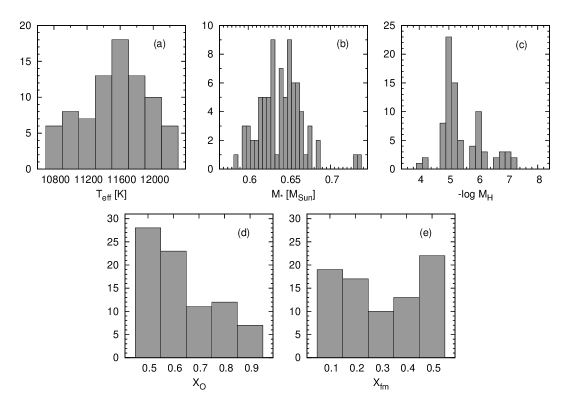
Figure 1: Histograms of the 81 selected models for the five physical parameters varied in the grid. The bin sizes are suited to the grid step sizes.

References

- Bischoff-Kim et al. (2008) A. Bischoff-Kim, M. H. Montgomery and D. E. Winget, ApJ 675, 1512–1517 (2008).
- Castanheira & Kepler (2009) B. G. Castanheira, S. O. Kepler, MNRAS 396, 1709–1731 (2009).
- Fontaine et al. (2001) G. Fontaine, P. Bergeron, P. Brassard, M. Billères and S. Charpinet, ApJ 557, 792–797 (2001).
- Kim (2007) A. Kim, Ph.D. thesis, University of Texas at Austin (2007).
- Kleinman et al. (1998) S. J. Kleinman, R. E. Nather, D. E. Winget et al., ApJ 495, 424–434 (1998).
- Koester et al. (2001) D. Koester, R. Napiwotzki, N. Christlieb et al., A&A 378, 556–568 (2001).
- Limoges & Bergeron (2010) M. M. Limoges, P. Bergeron, ApJ 714, 1037–1051 (2010).
- Yeates et al. (2005) C. M. Yeates, J. C. Clemens, S. E. Thompson and F. Mullally, ApJ 635, 1239–1262 (2005).