NORDITA-2015-72
UUITP-12/15

One-point Functions in Defect CFT and Integrability

Marius de Leeuw$\,{}^{1}$, Charlotte Kristjansen$\,{}^{1}$ and Konstantin Zarembo$\,{}^{2}$

¹ The Niels Bohr Institute, University of Copenhagen
Blegdamsvej 17, DK-2100 Copenhagen Ø, Denmark ² NORDITA, KTH Royal Institute of Technology and Stockholm University
Roslagstullsbacken 23, SE-106 91 Stockholm, Sweden
Department of Physics and Astronomy, Uppsala University
SE-751 08 Uppsala, Sweden

deleeuwm@nbi.ku.dk, kristjan@nbi.ku.dk, zarembo@nordita.org

Abstract

We calculate planar tree level one-point functions of  non-protected operators in the defect conformal field theory dual to the D3-D5 brane system with $k$ units of the world volume flux. Working in the operator basis of Bethe eigenstates of the Heisenberg $XXX_{1/2}$ spin chain we express the one-point functions as overlaps of these eigenstates with a matrix product state. For $k=2$ we obtain a closed expression of determinant form for any number of excitations, and in the case of half-filling we find a relation with the Néel state. In addition, we present a number of results for the limiting case $k\rightarrow\infty$.

1 Introduction

The simplest probes of external heavy objects in a conformal field theory, such as Wilson or ’t Hooft lines, surface operators or interfaces, are one-point functions of local operators in the presence of the defect. By conformal symmetry,

$$\left\langle\mathcal{O}(x)\right\rangle=\frac{C}{z^{\Delta}}\,,$$ (1.1)

where $z$ is the distance from $x$ to the defect and $\Delta$ is the scaling dimension of the operator $\mathcal{O}$. The constant $C$ in principle depends on the normalization of the operator at hand, but if the two-point function of $\mathcal{O}$ is unit-normalized, $C$ is defined unambiguously.

Here we focus on a domain wall in $\mathcal{N}=4$ Super-Yang-Mills (SYM) theory which separates vacua with $SU(N)$ and $SU(N-k)$ gauge groups [1]. This defect originates from the D3-D5 brane intersection and is dual to a probe D5 brane in $AdS_{5}\times S^{5}$ with $k$ units of electric flux on its world-volume [2]. One-point functions of chiral operators in this [3] and in the closely related D3-D7 defect CFT [4], when continued to strong coupling perfectly agree with the predictions of the AdS/CFT duality.

We would like to make a connection with integrability and will thus consider expectation values of non-protected operators. It has proven useful in this context to study operators of large bare dimension, which correspond to long quantum spin chains. Conformal operators of this type, due to operator mixing, are linear combinations of a large number of field monomials. Efficient calculation of the classical expectation values for such operators becomes a non-trivial problem, which can only be solved by employing the full machinery of the Bethe ansatz. The one-point correlators are probably the simplest objects sensitive to the structure of the Bethe wavefunctions, and are thus ideally suited to probe integrability beyond the spectral data.

2 Domain wall and spin chains

The D3-D5 intersection defect in $\mathcal{N}=4$ SYM has the following semiclassical description at weak coupling. On the one side of the domain wall, the gauge symmetry is broken from $SU(N)$ to $SU(N-k)$ by an infinite scalar vev. On the other side the scalar fields relax to zero according to their classical equations of motion:

$$\frac{d^{2}\Phi^{\rm cl}_{i}}{dz^{2}}=\left[\Phi^{\rm cl}_{j},\left[\Phi^{\rm cl}_{j},\Phi^{\rm cl}_{i}\right]\right].$$ (2.1)

For a supersymmetric defect, the solution also satisfies the first-order Nahm equations [5]:

$$\frac{d\Phi^{\rm cl}_{i}}{dz}=\frac{i}{2}\,\varepsilon_{ijk}\left[\Phi^{\rm cl}_{j},\Phi^{\rm cl}_{k}\right],$$ (2.2)

which automatically imply (2.1). The solution describing the D3-D5 intersection is [6, 7, 8]:

$$\Phi_{i}^{\rm cl}=\frac{1}{z}\,\begin{pmatrix}\left(t_{i}\right)_{k\times k}&0_{k\times(N-k)}\\ 0_{(N-k)\times k}&0_{(N-k)\times(N-k)}\\ \end{pmatrix},~{}i=1,2,3,\qquad\Phi^{\rm cl}_{i}=0,~{}i=4,5,6,$$ (2.3)

where the three $k\times k$ matrices $t_{i}$ satisfy

$$\left[t_{i},t_{j}\right]=i\varepsilon_{ijk}t_{k},$$ (2.4)

and consequently realize the unitary $k$-dimensional representation of $\mathfrak{su}(2)$.

The one-point functions, to the first approximation, are obtained by simply replacing quantum fields in the operator with their classical expectation values [3, 4]. To get a non-zero answer the operators must be built from scalar fields, and we will consider the most general such operators that do not contain derivatives:

$$\mathcal{O}=\Psi^{i_{1}\ldots i_{L}}\mathop{\mathrm{tr}}\Phi_{i_{1}}\ldots\Phi_{i_{L}}.$$ (2.5)

The $SO(6)$ tensor $\Psi$ is cyclically symmetric because of the trace condition.

These operators form a closed sector at one loop, and their mixing is described by an integrable $SO(6)$ spin-chain Hamiltonian, wherein the tensor $\Psi$ plays the role of the wave function in the spin-chain Hilbert space. The anomalous part of the dilatation generator (the mixing matrix) at one loop contains only nearest-neighbor interactions [9]:

$$\Gamma=\frac{\lambda}{16\pi^{2}}\sum_{l=1}^{L}H_{l,l+1},\qquad H_{lm}=2-2P_{lm}+K_{lm},$$ (2.6)

where $\lambda=g^{2}N$ is the ’t Hooft coupling of the SYM theory, and $P_{lm}$ and $K_{lm}$ are permutation and trace operators acting on sites $l$ and $m$ of the spin chain:

$$P_{ij}^{ks}=\delta^{k}_{j}\delta^{s}_{i},\qquad K_{ij}^{ks}=\delta_{ij}\delta^{ks}.$$ (2.7)

This result is not modified by the presence of the defect [10]. Notice, however, that the latter reference deals with a probe brane set-up without fluxes (corresponding to $k=0$) but the ultraviolet divergencies of the theory should be the same when the classical fields are turned on.

The Hamiltonian (2.6) is a member of an infinite hierarchy of commuting charges responsible for the integrability of the model. The third charge of the hierarchy acts on three neighboring spins:

$$Q_{3}=\sum_{l=1}^{L}Q_{l},\qquad Q_{l}=[H_{l-1,l},H_{l,l+1}].$$ (2.8)

Unlike the Hamiltonian, the third charge is parity-odd, and changes sign under the inversion of the spin chain orientation. The spectrum of the spin chain therefore contains parity pairs with degenerate energy and opposite values of $Q_{3}$, as well as unpaired states with vanishing $Q_{3}$.

The defect CFT contains also operators localized on the domain wall. These operators are described by an integrable open spin chain [10] and are dual to open strings with ends attached to the D5 brane. By considering one-point functions of the bulk operators we are, in a sense, dealing with the same string diagram but viewed as an absorption of a closed string by the D5 brane. In string theory the two descriptions should be related by $t-s$ channel duality, and it would be interesting to understand how they are related at weak coupling.

By substituting (2.3) into (2.5) we find that the one-point function is proportional to

$$\Psi^{i_{1}\ldots i_{L}}\mathop{\mathrm{tr}}t_{i_{1}}\ldots t_{i_{L}}\equiv\left\langle{\rm MPS}\,\right.\!\!\left|\vphantom{\Psi^{\rm cl}}\Psi\right\rangle,$$ (2.9)

the inner product of the spin-chain state $\Psi$ that characterizes the operator and the state with the wave function

$${\rm MPS}_{i_{1}\ldots i_{L}}=\mathop{\mathrm{tr}}t_{i_{1}}\ldots t_{i_{L}}.$$ (2.10)

MPS here stands for the ’Matrix Product State’, the term that will be explained below. The defect thus maps to a particular state in the spin-chain Hilbert space. We may interpret this state as a weak-coupling counterpart of the boundary state that describes the D5 brane in closed string theory. Recovering the normalization factor that makes the bulk two-point function of $\mathcal{O}$ unit-normalized, we get for the structure constant:

$$C=\left(\frac{8\pi^{2}}{\lambda}\right)^{\frac{L}{2}}L^{-\frac{1}{2}}\,\frac{\left\langle{\rm MPS}\,\right.\!\!\left|\vphantom{{\rm MPS}}\Psi\right\rangle}{\left\langle\Psi\right.\!\!\left|\Psi\right\rangle^{\frac{1}{2}}}.$$ (2.11)

What can be said about the state associated with the defect? It is not an eigenstate of the spin-chain Hamiltonian. We do not get anything nice when apply (2.6) to (2.10). However, the third charge of the integrable hierarchy acts in a simple way and actually annihilates the defect state:

$$Q_{3}\left|{\rm MPS}\right\rangle=0.$$ (2.12)

The proof is given in appendix A. This property leads to a selection rule for the one-point functions, since the overlap with MPS vanishes for all states that carry $Q_{3}\neq 0$.

To further simplify the problem we consider the $SU(2)$ subsector composed of operators which are built from two complex scalars

$$Z=\Phi_{1}+i\Phi_{4} \longleftrightarrow \left|\uparrow\right\rangle,$$

$$W=\Phi_{2}+i\Phi_{5} \longleftrightarrow \left|\downarrow\right\rangle.$$ (2.13)

The $SU(2)$ sector is closed to all loop orders, and at the leading order is described by the Heisenberg spin chain.

When restricted to the $SU(2)$ sector, the spin-chain state associated with the defect becomes

$$\left\langle{\rm MPS}\,\right|=\mathop{\mathrm{tr}}\nolimits_{a}\prod_{l=1}^{L}\left(\left\langle\uparrow_{l}\right|\otimes t_{1}+\left\langle\downarrow_{l}\right|\otimes t_{2}\right).$$ (2.14)

The index $a$ is introduced here to distinguish the “auxiliary” space of color indices of $t_{i}$ from the quantum space spanned by $\left|\uparrow\right\rangle$, $\left|\downarrow\right\rangle$ on each site of the spin chain. The defect state (2.14) can be obtained by applying an operator, which we can call the defect operator, to the ferromagnetic ground state of the spin chain:

$$\left\langle{\rm MPS}\,\right|=\left\langle\uparrow\ldots\uparrow\right|K.$$ (2.15)

The defect operator is not uniquely defined, because there are many operators that annihilate the ground state. We can choose it in the form

$$K=\mathop{\mathrm{tr}}\nolimits_{a}\prod_{l=1}^{L}\left\{\left[s\mathbbm{1}+(1-s)\sigma_{l}^{3}\right]\otimes t_{1}+\sigma^{+}_{l}\otimes t_{2}+\sigma^{-}_{l}\otimes t\right\},$$ (2.16)

where $\sigma^{i}_{l}$ are the Pauli matrices acting on the $l$-th site of the spin chain, $s$ is an arbitrary complex number, and $t$ can be any $k\times k$ matrix. For instance, taking $s=0$ and $t=t_{2}$, we find:

$$K=\mathop{\mathrm{tr}}\nolimits_{a}\prod_{l=1}^{L}\left(\sigma_{l}^{3}\otimes t_{1}+\sigma_{l}^{1}\otimes t_{2}\right),$$ (2.17)

which takes particularly simple form for $k=2$, with $t_{1}=\sigma^{3}/2$ and $t_{2}=\sigma^{1}/2$:

$$K^{\left(k=2\right)}=2^{-L}\mathop{\mathrm{tr}}\nolimits_{a}\prod_{l=1}^{L}\left(\sigma_{l}^{3}\otimes\sigma_{a}^{3}+\sigma_{l}^{1}\otimes\sigma_{a}^{1}\right).$$ (2.18)

States of the form (2.14) are known as the Matrix Product States, and were extensively studied in the condensed-matter literature [11, 12, 13, 14, 15, 16, 17, 18, 19, 20, 21], in particular to model quantum entanglement in one-dimensional systems. The operators (2.16), (2.17) and (2.18) are usually called the Matrix Product Operators.

In analogy to the algebraic Bethe ansatz (ABA) [22] the construction of the MPS uses the auxiliary space which threads through all sites of the spin chain. Interestingly, here the auxiliary space has a direct physical meaning of the color $SU(N)$ representation in the underlying gauge theory.

The conformal operators in the $SU(2)$ sector are labelled by zero-momentum eigenstates of the Heisenberg Hamiltonian. In the ABA framework, the eigenfunctions are constructed by applying creation operators $B(u)$ to the ferromagnetic vacuum of the spin chain:

$$\left|\left\{u_{j}\right\}\right\rangle=B(u_{1})\ldots B(u_{M})\left|0\right\rangle.$$ (2.19)

Each $B$-operator flips one spin, and for the state to be an eigenstate of the Heisenberg Hamiltonian the rapidities $\{u_{i}\}$ must fulfil the set of Bethe equations [22]. Our goal is to calculate the structure constant (2.11) for an arbitrary Bethe state of the form (2.19).

The trace cyclicity of the SYM operators imposes the zero-momentum constraint on the Bethe eigenstates. A simple way to fulfil this condition is to consider states in which rapidities come in pairs (the momentum is an odd function of $u$):

$$\left|\mathbf{u}\right\rangle=\left|u_{1}\ldots u_{\frac{M}{2}}\right\rangle\equiv\left|\left\{u_{j},-u_{j}\right\}\right\rangle.$$ (2.20)

Of course this way to impose the zero-momentum constraint is too restrictive and there are zero-momentum Bethe states in which rapidities are not balanced pairwise. These states form degenerate parity pairs related by reflection of all rapidities. Such paired states, however, carry a non-zero $Q_{3}$ and have zero overlap with the defect state as a consequence of (2.12). We can thus concentrate on the fully balanced, unpaired states of the form (2.20).

Our goal is to calculate

$$C_{\mathbf{u}}=\left(\frac{8\pi^{2}}{\lambda}\right)^{\frac{L}{2}}L^{-\frac{1}{2}}\,\frac{\left\langle{\rm MPS}\,|\mathbf{u}\right\rangle}{\left\langle\mathbf{u}\right.\!\!\left|\mathbf{u}\right\rangle^{\frac{1}{2}}}\,.$$ (2.21)

There is a considerable literature on overlaps of Bethe states in integrable systems (see [23, 24] for reviews), which in many cases admit compact determinant representation. The most famous examples are the Gaudin norm of an ABA state [25, 26], which is a part of the expression we need to evaluate, and the overlap of the on-shell and off-shell Bethe states [27]. Overlaps of Bethe states with MPS have not been studied so far, to the best of our knowledge. From known results the one that comes closest to our setup is the overlap of an arbitrary Bethe state with the Néel state, which was calculated in [28] and transformed into a convenient determinant form in [29, 30].

Bethe-state overlaps are playing an important rôle in the gauge/string integrability. The three-point functions in the $\mathcal{N}=4$ SYM at weak coupling can be expressed as generalized overlaps of Bethe states [31, 32, 33, 34, 35, 36, 37, 38, 39, 40, 41, 42, 43] and can be rendered into a compact determinant form [44, 45, 46, 47, 48], which is particularly useful in the semiclassical thermodynamic limit [33, 49, 50, 51, 52]. An interesting question is whether the one-point overlap (2.21) also admits a determinant representation.

In this paper we investigate this question in the simplest case when the auxiliary space has dimension two ($k=2$). We have found that the answer is affirmative, and moreover the result is given by exactly the same determinant formula as the overlap with the Néel state [29, 30], upon relaxing the half-filling condition $M=L/2$ necessary to make the Néel overlap non-zero. The final result is written in terms of the matrices of size $M/2\times M/2$:

$$K^{\pm}_{jk}=\frac{2}{1+\left(u_{j}-u_{k}\right)^{2}}\pm\frac{2}{1+\left(u_{j}+u_{k}\right)^{2}}\,,$$ (2.22)

and

$$G^{\pm}_{jk}=\left(\frac{L}{u_{j}^{2}+\frac{1}{4}}-\sum_{n}K^{+}_{jn}\right)\delta_{jk}+K^{\pm}_{jk}.$$ (2.23)

The structure constant (2.21) is given by the ratio of two determinants:

$$C_{\mathbf{u}}=2\left[\left(\frac{2\pi^{2}}{\lambda}\right)^{L}\,\frac{1}{L}\,\prod_{j}\frac{u_{j}^{2}+\frac{1}{4}}{u_{j}^{2}}\,\,\frac{\det G^{+}}{\det G^{-}}\right]^{\frac{1}{2}}.$$ (2.24)

When $M=L/2$, this formula coincides exactly with the expression for overlap between a half-filled Bethe eigenstate and the Néel state given in [29, 30]. Although the MPS is different from the Néel state, even if restricted to equal number of up and down spins, this is not a coincidence. We were able to show that the MPS is cohomologically equivalent to the Néel state at half filling and consequently has the same overlaps with all half-filled Bethe eigenstates. The result above then follows from the derivation in [28, 29, 30], for $M=L/2$. When $M<L/2$, this formula is a conjecture which we have extensively checked. We have also identified a natural generalization of the Néel state away from half-filling, which lies in the same cohomology class as the definite-spin projection of MPS.

In section 3 we introduce the tools necessary for our computation, namely the Bethe ansatz and an explicit realization of a set of $k\times k$ matrices which constitute a unitary $k$-dimensional representation of $SU(2)$. Subsequently, in section 4 we sketch our computations and present the results. In section 5 we discuss the relationship between the MPS and the Néel state and introduce generalized Néel states with unequal number of up and down spins. Section 6 contains a discussion of the thermodynamical limit and section 7 some comments on the string theory observables dual to the one-point functions of the defect CFT. Finally section 8 contains our conclusion.

3 Setting up the computation

Although the construction of the defect state has a strong resemblance with certain elements of the algebraic Bethe ansatz we have found it most convenient to evaluate the overlaps by using the Bethe ansatz in its coordinate space version which we will summarize below, see for instance [53, 54]. Hereafter we will present the explicit representations of $SU(2)$ that we will make use of in our computations.

3.1 The coordinate Bethe Ansatz

The eigenstates of the dilatation operator restricted to the $SU(2)$ sector are in one-to-one correspondence with eigenstates of the Heisenberg XXX spin chain. In this section we introduce this model and discuss its solution via the coordinate Bethe ansatz.

Model

The XXX spin chain is a one-dimensional lattice model consisting of $L$ spin-${\textstyle\frac{1}{2}}$ particles. Therefore, the Hilbert space is $\bigotimes_{L}\mathbb{C}^{2}$, where each $\mathbb{C}^{2}$ is spanned by $|\!\uparrow\rangle,|\!\downarrow\rangle$. The Hamiltonian describes a standard nearest neighbor spin-spin interaction

$$\mathcal{H}=\sum_{i=1}^{L}\mathcal{H}_{ii+1}, \mathcal{H}_{ij}=\frac{1}{4}-\vec{S}_{i}\cdot\vec{S}_{j},$$ (3.1)

with periodic boundary conditions $L+1\equiv 1$. For simplicity let us also introduce the the usual raising and lowering operators $S^{\pm}$ such that

$$S^{+}|\!\downarrow\rangle=|\!\uparrow\rangle, S^{-}|\!\uparrow\rangle=|\!\downarrow\rangle.$$ (3.2)

Expressing the permutation operator in terms of spin operators one can see that (2.6) reduces to (3.1) in the $SU(2)$ subsector, up to normalization. The (coordinate) Bethe ansatz gives us a method to diagonalize this Hamiltonian and to compute its spectrum.

Bethe eigenstates

The first step of the Bethe ansatz is to introduce a vacuum state

$$|0\rangle=\bigotimes_{i=1}^{L}|\!\uparrow\rangle.$$ (3.3)

This vacuum state is trivially an eigenstate of the Hamiltonian. The other eigenstates will also have down-spins on various sites. The Bethe ansatz postulates that these eigenstates are of a plane wave type. More precisely, each flipped spin behaves like a quasi-particle referred to as a magnon. These magnons propagate along the spin chain with some definite momentum $p$. The Bethe eigenstate for a chain of length $L$ describing $M$ magnons, is of the form

$$|\vec{p}\rangle:=|p_{1},\ldots,p_{M}\rangle=N\sum_{\sigma\in S_{M}}\sum_{1\leqslant n_{1}<\ldots<n_{M}\leqslant L}e^{i\sum_{m}(p_{\sigma_{m}}n_{m}+\sum_{j<m}\frac{\theta_{\sigma_{j}\sigma_{m}}}{2})}S^{-}_{n_{1}}\ldots S^{-}_{n_{M}}|0\rangle,$$ (3.4)

where $N$ is an overall normalization. The sum over $\sigma$ runs over all permutations of $M$ elements. Furthermore, the factors $\theta$ parameterize the two-magnon S-matrix via

$$\mathcal{S}_{ij}:=e^{\theta_{ij}-\theta_{ji}}=-\frac{1+e^{ip_{i}+ip_{j}}-2e^{ip_{i}}}{1+e^{ip_{i}+ip_{j}}-2e^{ip_{j}}}.$$ (3.5)

It is worthwhile to note that, up to an overall normalization, the Bethe vector (3.4) only depends on the S-matrix $\mathcal{S}$ rather than the phase $\theta$. In the remainder we will choose the normalization $N$ such that the term $e^{ip_{i}n_{i}}$ (i.e. the term with $\sigma=1$) in (3.4) appears with unit coefficient. In other words, we will set $N=e^{-\sum_{j<k}\theta_{jk}/2}$.

Bethe equations

Finally, the state (3.4) should respect the correct boundary conditions, i.e. it should be periodic. Imposing periodicity results in a set of equations on the momenta of the magnons, called the Bethe equations

$$e^{ip_{k}L}=\prod_{i\neq k}\mathcal{S}_{ki}.$$ (3.6)

When the momenta satisfy these Bethe ansatz equations, it is easy to check that the state (3.4) is an eigenstate of the Hamiltonian with eigenvalue

$$E=2\sum_{i=1}^{M}\sin^{2}\frac{p_{i}}{2}=\frac{1}{2}\sum_{i=1}^{M}\frac{1}{u_{i}^{2}+\frac{1}{4}},$$ (3.7)

where $u=\frac{1}{2}\cot(p/2)$ is the rapidity. In order for a Bethe eigenstate to represent a single trace gauge theory operator it is furthermore necessary that the momenta of its excitations add up to an integer multiple of $2\pi$. This is required to account for the cyclicity properties of the trace, i.e.

$$P\equiv\sum_{i=1}^{M}p_{i}=2\pi m.$$ (3.8)

Finally, notice that our Bethe states (3.4) (with $N=e^{-\sum_{j<k}\theta_{jk}/2}$) are not normalized to unity. These coordinate space Bethe eigenstates can be related to the eigenstates of the algebraic Bethe ansatz approach in the following way (see, for example, [31])

$$|\{u_{i}\}\rangle =B(u_{1})\ldots B(u_{M})|0\rangle$$

$$=\prod_{j}\left(u_{j}-\frac{i}{2}\right)^{L}\left(\frac{i}{u_{j}+\frac{i}{2}}\right)\prod_{l<m}\left(1+\frac{i}{u_{l}-u_{m}}\right)|p_{1},\ldots,p_{M}\rangle.$$ (3.9)

This, in conjunction with the Gaudin formula [25, 26] for the norm of $|\{u_{i}\}\rangle$, fixes the normalization of coordinate Bethe ansatz eigenstates.

Overlap

Let us now continue by computing the overlap between the Bethe states and the defect state $\langle{\rm MPS}\,|\vec{p}\rangle$. Inserting the $M$-magnon state (3.4) into (2.9) yields

$$\langle{\rm MPS}\,|\vec{p}\rangle=N\sum_{\sigma\in S_{M}}\sum_{1\leqslant n_{1}<\ldots<n_{M}\leqslant L}e^{ip_{\sigma(i)}n_{i}+\sum_{j<i}{\textstyle\frac{i}{2}}\theta_{\sigma(j)\sigma(i)}}\,\mathrm{tr}[t_{1}^{n_{1}-1}t_{2}t_{1}^{n_{2}-n_{1}-1}\ldots],$$ (3.10)

where the $t_{i}$ form the standard $k$-dimensional irreducible representation of $\mathfrak{su}(2)$. However, for practical computations it is more convenient to take

$$\langle{\rm MPS}\,|\vec{p}\rangle=N\sum_{\sigma\in S_{M}}\sum_{1\leqslant n_{1}<\ldots<n_{M}\leqslant L}e^{ip_{\sigma(i)}n_{i}+\sum_{j<i}{\textstyle\frac{i}{2}}\theta_{\sigma(j)\sigma(i)}}\,\mathrm{tr}[t_{3}^{n_{1}-1}t_{1}t_{3}^{n_{2}-n_{1}-1}\ldots],$$ (3.11)

which will clearly yield the same results.

3.2 Representations of $\mathfrak{su}(2)$

Let us spell out the explicit representation for the $\mathfrak{su}(2)$ generators $t_{i}$ that we will use and derive some useful relations.

Definition

Consider the $k$-dimensional complex vector space generated by the basis vectors $E_{i}$. Define the standard matrix unities $E^{i}{}_{j}$ that are zero everywhere except for a 1 at position $(i,j)$, such that they satisfy

$$E^{i}{}_{j}E^{k}{}_{l}=\delta^{k}{}_{j}E^{i}{}_{l}.$$ (3.12)

If we introduce the following constants

$$c_{k,i}=\sqrt{i(k-i)}, d_{k,i}={\textstyle\frac{1}{2}}(k-2i+1),$$ (3.13)

and consider the matrices

$$t_{+}:=\sum_{i=1}^{k-1}c_{k,i}E^{i}{}_{i+1}, t_{-}:=\sum_{i=1}^{k-1}c_{k,i}E^{i+1}{}_{i}, t_{3}:=\sum_{i=1}^{k}d_{k,i}E^{i}{}_{i},$$ (3.14)

then we obtain the standard $k$-dimensional $\mathfrak{su}(2)$ representation by defining

$$t_{1}=\frac{t_{+}+t_{-}}{2}, t_{2}=\frac{t_{+}-t_{-}}{2i}.$$ (3.15)

It is easy to check that these matrices satisfy the $\mathfrak{su}(2)$ commutation relations (2.4). Note that all these matrices are traceless.

Automorphisms

Let us introduce two similarity transformations

$$U=U^{-1}:=\sum_{i=1}^{k}E^{i}{}_{k-i+1}, V=V^{-1}:=\sum_{i=1}^{k}(-1)^{i}E^{i}{}_{i}.$$ (3.16)

It is easy to show that under these transformations

$$Ut_{1}U^{-1}=t_{1}, Ut_{2,3}U^{-1}=-t_{2,3} Vt_{3}V^{-1}=t_{3}, Vt_{1,2}V^{-1}=-t_{1,2}.$$ (3.17)

Hence, they provide a trivial automorphism of the algebra.

4 Results

In this section we present a number of explicit results for the overlap (3.11).

4.1 $L$ or $M$ odd

If $L$ or $M$ is odd, the overlap vanishes. This follows directly from the automorphisms (3.16). Indeed, for any state of the form $\mathrm{tr}[t_{3}^{n_{1}}t_{1}t_{3}^{n_{2}}\ldots]$, containing $M$ $t_{1}$’s and $L$ $t$’s we have by cyclicity of the trace

$$\mathrm{tr}[t_{3}^{n_{1}}t_{1}t_{3}^{n_{2}}\ldots]=\mathrm{tr}[(Ut_{3}U^{-1})^{n_{1}}Ut_{1}U^{-1}(Ut_{3}U^{-1})^{n_{2}}\ldots]=(-1)^{L-M}\mathrm{tr}[t_{3}^{n_{1}}\ldots]$$ (4.1)

and

$$\mathrm{tr}[t_{3}^{n_{1}}t_{1}t_{3}^{n_{2}}\ldots]=\mathrm{tr}[(Vt_{3}V^{-1})^{n_{1}}Vt_{1}V^{-1}(Vt_{3}V^{-1})^{n_{2}}\ldots]=(-1)^{M}\mathrm{tr}[t_{3}^{n_{1}}\ldots].$$ (4.2)

This implies that the expression $\mathrm{tr}[t_{3}^{n_{1}}t_{1}t_{3}^{n_{2}}\ldots]$, and hence the overlap (3.11), is only non-vanishing if $L$ and $M$ are both even.

4.2 Vacuum, $M=0$

From (3.14) we see that $t_{3}$ is a diagonal matrix with entries ${\textstyle\frac{1}{2}}(k-2i+1)$ for $i=1,\ldots,{k}$. From this, it immediately follows that for the vacuum state (3.3) the overlap (3.11) reduces to

$$\langle{\rm MPS}\,|0\rangle=\mathrm{tr}\,t_{3}^{L}=\sum_{i=1}^{k}d_{k,i}^{L}.$$ (4.3)

The resulting sum can be evaluated to a combination of $\zeta$-functions

$$\langle{\rm MPS}\,|0\rangle=\zeta_{-L}({\textstyle\frac{1-k}{2}})-\zeta_{-L}({\textstyle\frac{1+k}{2}}).$$ (4.4)

Taking the $k\rightarrow\infty$ limit of the explicit expression for $\langle{\rm MPS}\,|0\rangle$ yields

$$\langle{\rm MPS}\,|0\rangle=\frac{k^{L+1}}{2^{L}(L+1)}+\mathcal{O}(k^{L})\qquad\left(k\rightarrow\infty\right).$$ (4.5)

This agrees with the large $k$ behavior which was found previously in [3, 4].

4.3 Excited states

4.3.1 General considerations

We first notice that the defect state $\left|{\rm MPS}\rangle\right.$ is a cyclically invariant state (due to the cyclic nature of its expansion coefficients). This implies that

$$\left(\left\langle{\rm MPS}\right.\left|\vphantom{{\rm MPS}}\,U\right)\,\right|\left.\vphantom{{\rm MPS}}\vec{p}\right\rangle=\left\langle{\rm MPS}\right.\left|\vphantom{{\rm MPS}}\right.\left.\vphantom{{\rm MPS}}\vec{p}\right\rangle=\left\langle{\rm MPS}\right.\left|\vphantom{\Psi^{\rm cl}}\,\left(\vphantom{{\rm MPS}}U\,\right|\left.\vec{p}\vphantom{{\rm MPS}}\right\rangle\right),$$ (4.6)

where $U=e^{i\hat{P}}$ is the lattice translation operator and $\hat{P}$ the momentum operator. From this we conclude that the overlap vanishes unless $\left|\vec{p}\right\rangle$ is a zero-momentum state.

Secondly, we notice that for an even number of excitations $\left|{\rm MPS}\rangle\right.$ is invariant under an operation traditionally denoted as parity, see for instance [55]. Its action on a spin state is defined by

$${\cal P}\left.\left|{\mathfrak{t}}_{1}{\mathfrak{t}}_{2}\ldots{\mathfrak{t}}_{n}\right.\right\rangle=\left.\left|{\mathfrak{t}}_{n}{\mathfrak{t}}_{n-1}\ldots{\mathfrak{t}}_{1}\right.\right\rangle,$$ (4.7)

where ${\mathfrak{t}}_{i}\in\{\downarrow,\uparrow\}$. The invariance of $\left|{\rm MPS}\rangle\right.$under this transformation follows from the invariance of its expansion coefficients under a similar operation performed on the matrices inside the traces. By an argument similar to the one above it follows that the overlap vanishes unless the Bethe eigenstate has positive parity. It is well-known that the eigenstates of the Heisenberg spin chain can be chosen to be eigenstates of a definite parity. In particular, the so-called un-paired eigenstates for which the Bethe rapidities fulfill that $\{u_{i}\}=\{-u_{i}\}$ are automatically eigenstates with parity equal to $(-1)^{M(L+1)}$. Moreover, as discussed in section 2, we find that only these unpaired state can have a non-trivial overlap with the classical function. This follows from the fact that the unpaired states are exactly the states that are annihilated by the odd charges $Q_{2n+1}$.

4.3.2 Two excitations, $M=2$

By using the cyclicity of the trace, we can rewrite the overlap (3.11) as a sum of terms of the form

$$\mathrm{tr}[t_{3}^{L-m-1}t_{1}t_{3}^{m-1}t_{1}].$$ (4.8)

We can evaluate this trace by implementing the explicit expressions for $t_{i}$ (3.14)

$$\mathrm{tr}[t_{3}^{L-m-1}t_{1}t_{3}^{m-1}t_{1}]= \sum_{a,b=1}^{k}\sum_{i,j=1}^{k-1}\frac{1}{4}d_{k,a}^{L-m-1}d_{k,b}^{m-1}c_{k,i}c_{k,j}$$

$$\qquad\mathrm{tr}[E^{a}{}_{a}\left(E^{i}{}_{i+1}+E^{i+1}{}_{i}\right)E^{b}{}_{b}\left(E^{j}{}_{j+1}+E^{j+1}{}_{j}\right)].$$ (4.9)

The definition of the matrix unities then allows us to work out the trace

$$\mathrm{tr}[t_{3}^{L-m-1}t_{1}t_{3}^{m-1}t_{1}] =2^{1-L}\sum_{i=1}^{k-1}\frac{i(k-i)}{(k-2i)^{2}-1}\left[\frac{k-2i+1}{k-2i-1}\right]^{m}(k-2i-1)^{L}.$$ (4.10)

Thus, for $M=2$, the Bethe states are mapped to

$$\langle{\rm MPS}\,|p_{1},p_{2}\rangle =\sum_{m<n}[e^{i(p_{1}n+p_{2}m)}+\mathcal{S}_{21}e^{i(p_{2}n+p_{1}m)}]\mathrm{tr}[t_{3}^{m-1}t_{1}t_{3}^{n-m-1}t_{1}t_{3}^{L-n}]$$

$$=\sum_{m<n}[e^{i(p_{1}n+p_{2}m)}+\mathcal{S}_{21}e^{i(p_{2}n+p_{1}m)}]\mathrm{tr}[t_{3}^{L-n+m-1}t_{1}t_{3}^{n-m-1}t_{1}].$$ (4.11)

The sums over $m,n$ can easily be done and we find the following formula for the overlap

$$\langle{\rm MPS}\,|p_{1},p_{2}\rangle=\frac{e^{i(p_{1}+p_{2})}}{1-e^{i(p_{1}+p_{2})}}\sum_{i=1}^{k-1}\frac{i(k-i)}{2^{L-1}(k-2i-1)^{2-L}}\left[e^{ip_{2}}\frac{e^{iLp_{2}}\left[\frac{k-2i+1}{k-2i-1}\right]^{L}-1}{e^{ip_{2}}\left[\frac{k-2i+1}{k-2i-1}\right]-1}-\right.$$ (4.12)

$$\left.e^{iLp_{2}}\frac{e^{iLp_{1}}-\left[\frac{k-2i+1}{k-2i-1}\right]^{L}}{e^{ip_{1}}-\left[\frac{k-2i+1}{k-2i-1}\right]}+\mathcal{S}_{21}e^{ip_{1}}\frac{e^{iLp_{1}}\left[\frac{k-2i+1}{k-2i-1}\right]^{L}-1}{e^{ip_{1}}\left[\frac{k-2i+1}{k-2i-1}\right]-1}-\mathcal{S}_{21}e^{iLp_{1}}\frac{e^{iLp_{2}}-\left[\frac{k-2i+1}{k-2i-1}\right]^{L}}{e^{ip_{2}}-\left[\frac{k-2i+1}{k-2i-1}\right]}\right].$$

Notice that the above expression has to be evaluated with care in case $k$ is odd due to a superficial pole at $i={\textstyle\frac{1}{2}}(k-1)$. By using that $\langle{\rm MPS}\,|p_{1},p_{2}\rangle$ is invariant if we redefine the summation via $i\rightarrow k-i$ it is easy to check that upon substituting the Bethe equations (3.6) the overlap vanishes unless $p_{1}+p_{2}=0$ where the above expression has a pole. Then, imposing the vanishing of the total momentum and setting $p_{1}=-p_{2}=p$ from the beginning gives us the following one-point function

$$\langle{\rm MPS}\,|p,-p\rangle=Lu(u-{\textstyle\frac{i}{2}})\sum_{j=-\frac{k}{2}}^{\frac{k}{2}}\frac{j^{2}-\frac{k^{2}}{4}}{j^{2}+u^{2}}(j-{\textstyle\frac{1}{2}})^{L-1}.$$ (4.13)

For $k=2$ this reduces to $2^{1-L}\,Lu^{-1}(u-{\textstyle\frac{i}{2}})$.

4.3.3 General $M$

In the following we will derive some results for a general even number of excitations $M$. In particular, for the case $k=2$, we will give a closed formula of determinant form, valid for any even $M$.

$k=2$

For $k=2$ computing the overlap simplifies due to the identities

$$t_{i}^{2}={\textstyle\frac{1}{4}}, \{t_{i},t_{j}\}=0,\qquad i\neq j.$$ (4.14)

The anti-commutator identity means that we can order the generators in the trace (possibly at the cost of a sign) and the first identity implies that we can take all the powers in the trace mod 2. In particular, we can simplify (3.11) to

$$\langle{\rm MPS}\,|\vec{p}\rangle_{k=2} =N\sum_{\sigma\in S_{M}}\sum_{1\leqslant n_{1}<\ldots<n_{M}\leqslant L}e^{ip_{\sigma(i)}n_{i}+\sum_{j<i}{\textstyle\frac{i}{2}}\theta_{\sigma(j)\sigma(i)}}\,(-1)^{\sum_{i}n_{i}+\frac{M}{2}}\mathrm{tr}[t_{1}^{L-M}t_{2}^{M}],$$

$$=\frac{(-1)^{M/2}N}{2^{L}}\sum_{\sigma\in S_{M}}\sum_{1\leqslant n_{1}<\ldots<n_{M}\leqslant L}e^{i(p_{\sigma(i)}+\pi)n_{i}+\sum_{j<i}{\textstyle\frac{i}{2}}\theta_{\sigma(j)\sigma(i)}},$$

$$=\frac{(-1)^{M/2}N}{2^{L}}\sum_{\sigma\in S_{M}}e^{\sum_{j<i}{\textstyle\frac{i}{2}}\theta_{\sigma(j)\sigma(i)}}\sum_{1\leqslant n_{1}<\ldots<n_{M}\leqslant L}e^{i(p_{\sigma(i)}+\pi)n_{i}}.$$ (4.15)

The above sum can be evaluated as follows

$$\sum_{1\leqslant n_{1}<\ldots<n_{M}\leqslant L}x_{1}^{n_{1}}\ldots x_{M}^{n_{M}}=$$ (4.16)

$$\hskip 56.9055pt\prod_{n=1}^{M}x_{n}^{L+1}+\sum_{a=1}^{M}\!\left[\!1-\prod_{n=1}^{a}x_{n}^{L+1}\!\right]\!\!\left[\!\prod_{m=1}^{a}\frac{x_{m}^{m}}{1-\prod_{n=m}^{a}x_{n}}\!\right]\!\!\left[\!\prod_{m=a+1}^{M}\frac{x_{m}^{L+1}}{\prod_{n=a+1}^{m}x_{n}-1}\!\right].$$

In agreement with our general discussion, cf.  section 2, we find that the only Bethe eigenstates that give a non-zero overlap function are states with momentum configurations of the form

$$(p_{1},-p_{1},p_{2},-p_{2},\ldots,p_{\frac{M}{2}},-p_{\frac{M}{2}}).$$ (4.17)

For these states one can write the overlap function in a compact form as the determinant of a matrix. Define the following function

$$K_{ij}:=\frac{1}{2}\left[\frac{1+4u_{i}^{2}}{1+(u_{i}+u_{j})^{2}}+\frac{1+4u_{i}^{2}}{1+(u_{i}-u_{j})^{2}}\right],$$ (4.18)

and the following $M/2\times M/2$ matrix

$$A_{ij}:=(L-\sum_{n=1}^{M/2}K_{in})\delta_{ij}+K_{ij},$$ (4.19)

then the overlap function is given by

$$\langle{\rm MPS}\,|\vec{p}\rangle_{k=2}=2^{1-L}(\det A)\prod_{i=1}^{M/2}\frac{u_{i}-{\textstyle\frac{i}{2}}}{u_{i}}.$$ (4.20)

We have confirmed this formula by explicit computations up to and including the case of eight excitations. Upon translating to the algebraic Bethe ansatz framework (cf. (3.1)), using the Gaudin formula for the norm, and applying elementary determinant identities, we arrive at the aforementioned result (2.24).

Large $k$

Let us have a closer look at the leading order large $k$ expansion for any number of excitations. One can show that for $M$ excitations

$$\mathrm{tr}(t_{3}^{n_{1}-1}t_{1}t_{3}^{n_{2}-n_{1}-1}t_{1}\ldots)=-\frac{\sqrt{\pi}\,\Gamma\left(-\frac{L+1}{2}\right)}{\Gamma\left(\frac{1-M}{2}\right)\Gamma\left(\frac{1-L+M}{2}\right)}k^{L+1}+\mathcal{O}(k^{L}).$$ (4.21)

This can be seen as follows. First, in the large $k$ limit $\mathrm{tr}(t_{3}^{L-M}(t_{+}t_{-})^{\frac{M}{2}})$ can be rewritten as a Riemann sum and integration then leads to the following identity

$$\mathrm{tr}(t_{3}^{L-M}(t_{+}t_{-})^{\frac{M}{2}})=-\frac{\sqrt{\pi}\,\Gamma\left(-\frac{L+1}{2}\right)}{\binom{M}{\frac{M}{2}}\Gamma\left(\frac{1-M}{2}\right)\Gamma\left(\frac{1-L+M}{2}\right)}\frac{k^{L+1}}{\binom{M}{\frac{M}{2}}2^{L+1}}+\mathcal{O}(k^{L}).$$ (4.22)

Second, from the defining commutation relations of $\mathfrak{su}(2)$ it can be seen that any distribution of $t_{3},t_{\pm}$ under the trace can be ordered as (4.22) at the cost of terms of lower order in $k$. Then (4.21) follows by expressing $t_{1}$ in terms of $t_{\pm}$ as in (3.15).

This means that the large $k$ limit of the overlap function reduces to

$$\langle{\rm MPS}\,|\vec{p}\rangle=-\sqrt{\pi}\frac{N\,\Gamma\left(-\frac{L+1}{2}\right)}{\Gamma\left(\frac{1-M}{2}\right)\Gamma\left(\frac{1-L+M}{2}\right)}\frac{k^{L+1}}{2^{L}}\sum_{\sigma\in S_{M}}\sum_{1\leqslant n_{1}<\ldots<n_{M}\leqslant L}e^{ip_{\sigma(i)}n_{i}+\sum_{j<i}{\textstyle\frac{i}{2}}\theta_{\sigma(j)\sigma(i)}}.$$ (4.23)

It is easy to check that for $M=0$ it reduces to the large $k$ behavior we found for the vacuum state (4.5). However, for $M\neq 0$ something unusual happens.

Notice that (4.23) can be expressed as the inner product of the Bethe state (3.4) with the fully symmetrized state that has $M$ spins down. Such a state can be expressed as the lowering operator $S^{-}$ acting on vacuum $M$ times, i.e. $\Delta^{(L)}(S^{-})^{M}|0\rangle$. Thus, we can re-express the overlap as

$$\langle{\rm MPS}\,|\vec{p}\rangle=\langle 0|\Delta^{(L)}(S^{+})^{M}|\vec{p}\rangle,$$ (4.24)

where $\Delta$ is the coproduct. However, due to the fact that Bethe states are highest weight states, the above vanishes. In other words, the inclusion of excitations lowers the order of the overlap for large $k$.

In order to gain a better understanding of this phenomenon, let us look at the large $k$ behavior for $M=0,2,4$. We study the large $k$ behavior by explicitly evaluating the relevant overlap function for a large range of values of $L,k$. The overlap will be a polynomial in $k$ of degree at most $L+1$ with coefficients that are rational functions of $L$. Letting $L$ run from 2 to $20$ and $k$ from $2$ to $30$ allowed us to fix the relevant coefficients. In general, we find that the large $k$ behavior is of the form

$$\langle{\rm MPS}\,|\vec{p}\rangle= N\sum_{\sigma}\sum_{n_{i}}\,\sum_{m=0}\beta^{(m)}_{L,M}(n_{i})k^{L+1-m}\,e^{ip_{\sigma(i)}n_{i}+\sum_{j<i}{\textstyle\frac{i}{2}}\theta_{\sigma(j)\sigma(i)}}.$$ (4.25)

The coefficient $\beta^{(0)}$ is constant and can be read off from (4.23). For $M=0$ the first few $\beta^{(m)}$ are constant and from (4.4) the large $k$ behavior is easily found to be

$$\langle{\rm MPS}\,|0\rangle=\frac{1}{2^{L}}\left(\frac{k^{L+1}}{L+1}-\frac{1}{6}L\,k^{L-1}+\frac{7}{360}(L-2)(L-1)L\,k^{L-3}+\mathcal{O}(k^{L-5})\right).$$ (4.26)

Notice that the even orders vanish.

However, starting from $M=2$ the coefficients become non-trivial. Let us list the first few $\beta^{(m)}_{L,2}$ and describe their contribution. If we denote $n_{ij}=n_{i}-n_{j}$, then

$$\beta^{(1)}_{L,2}=\frac{2^{-L}}{L-1},$$ (4.27)

$$\beta^{(2)}_{L,2}=\frac{2^{1-L}}{L-3}\left[\frac{L}{3}+\frac{n_{12}(L+n_{12})}{L-1}\right]$$ (4.28)

$$\beta^{(3)}_{L,2}=\frac{L(L+1)+6\,n_{12}(L+n_{12})}{3\cdot 2^{L}(L-3)}$$ (4.29)

$$\ \beta^{(4)}_{L,2}=\frac{2^{1-L}}{L-5}\left[\frac{(L-2)L(L+3)}{30}+\frac{(L^{2}-4L+5)n_{12}(L+n_{12})}{3(L-3)}+\frac{n_{12}^{2}(L+n_{12})^{2}}{3(L-3)}\right]$$ (4.30)

Since $\beta^{(1)}_{L,2}$ is constant it vanishes by the same arguments as the leading order. For the other terms, the factors of $n_{i}$ can be written as derivatives of momenta $p_{i}$ when calculating the explicit overlap function. This allows us to evaluate the overlap (4.25) to the relevant order. Again we find that upon using the Bethe equations that it vanishes unless we impose pairwise momentum conservation. Doing this, we find for the next two terms

$$\langle{\rm MPS}\,|p,-p\rangle =\frac{u(u+{\textstyle\frac{i}{2}})L}{L-3}\left[\frac{k^{L-1}}{2^{L-2}}+(L-1)\frac{k^{L-2}}{2^{L-2}}+\mathcal{O}(k^{L-3})\right]$$ (4.31)

Notice that, in contradistinction to the vacuum, there is a contribution at an even order. Finally, the next non-trivial contribution is

$$\langle{\rm MPS}\,|p,-p\rangle_{\mathcal{O}(k^{L-3})}= \frac{2^{2-L}L(L-1)}{3(L-3)(L-5)}u(u+{\textstyle\frac{i}{2}})[L(L-11)-12u^{2}].$$ (4.32)

Starting from $k^{L-1}$ terms appear at both even and odd orders.

Next, we turn to four excitations $M=4$. It can be shown that the first order for $M=4$ particles that contributes is $k^{L-3}$. This seems to indicate that the order at which the large $k$ expansion begins is $k^{L-M+1}$. The first non-trivial coefficient for four particles can be computed along the same lines as for $M=2$ and we find

$$\frac{u_{1}(u_{1}+{\textstyle\frac{i}{2}})u_{2}(u_{2}+{\textstyle\frac{i}{2}})}{2^{L-4}}\frac{L}{L-7}\left[L-4+\frac{2(1+u_{2}^{4}+u_{1}^{2}(1-8u_{2}^{2}))}{(1+(u_{1}+u_{2})^{2})(1+(u_{1}-u_{2})^{2})}\right]\,k^{L-3}$$ (4.33)

The general structure of the contributions is indicated in Table 1.

	$k^{L+1}$	$k^{L}$	$k^{L-1}$	$k^{L-2}$	$k^{L-3}$
$M=0$	$\star$	0	$\star$	0	$\star$
$M=2$	0	0	$\star$	$\star$	$\star$
$M=4$	0	0	0	0	$\star$

Table 1: Large $k$ behavior of the one-point functions for $M=0,2,4$ excitations. The order at which the expansion starts is $k^{L+1-M}$.

5 Matrix product and Néel states

In this section we elucidate the relationship between the matrix product and the Néel states. This will allow us to prove equation (2.24) for $M=L/2$. The Néel state is the vacuum of the classical (Ising) anti-ferromagnet:

$$\left|{\rm N\acute{e}el}\right\rangle=\left|\uparrow\downarrow\uparrow\downarrow\ldots\uparrow\downarrow\right\rangle+\left|\downarrow\uparrow\downarrow\uparrow\ldots\downarrow\uparrow\right\rangle.$$ (5.1)

The state has equal number of up and down spins (we assume that the length $L$ of the spin chain is even).

On the other hand, the matrix product state has components with any even number of up and down spins. Since the total spin in conserved, it is convenient to decompose this state into components with definite number of up and down spins. Let us denote the projector onto states with $M$ down spins by $P_{M}$, and select the definite-spin component of the MPS (2.14) by

$$\left|{\rm MPS}_{M}\right\rangle=P_{M}\left|{\rm MPS}\right\rangle.$$ (5.2)

To facilitate the bookkeeping, it is convenient to introduce the generalized MPS:

$$\left|{\rm MPS}(z)\right\rangle=\mathop{\mathrm{tr}}_{a}\prod_{l=1}^{L}\left(t_{1}\left|\uparrow_{l}\right\rangle+zt_{2}\left|\downarrow_{l}\right\rangle\right)$$ (5.3)

where $z$ is a complex number. Then,

$$\left|{\rm MPS}_{M}\right\rangle=\oint\frac{dz}{2\pi iz^{M+1}}\,\left|{\rm MPS}(z)\right\rangle.$$ (5.4)

We can also generalize the Néel state to the case of an arbitrary even number of down spins:

$$\left|{\rm N\acute{e}el}_{M}\right\rangle=\sum_{{{l_{1}<\ldots<l_{M}}\atop{|l_{i}-l_{j}|\,-\,{\rm even}}}}\left|\uparrow\ldots\uparrow\underset{l_{1}}{\downarrow}\uparrow\ldots\underset{l_{2}}{\downarrow}\ldots\underset{l_{M}}{\downarrow}\ldots\uparrow\right\rangle.$$ (5.5)

This looks like a descendant of the ground state, and would have been such, if not for the constraint that spin-flips hop by an even number of sites. Obviously,

$$\left|{\rm N\acute{e}el}\right\rangle=\left|{\rm N\acute{e}el}_{\frac{L}{2}}\right\rangle.$$ (5.6)

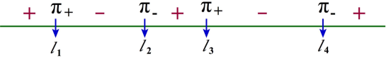
Figure 1: The generalized MPS state (5.7).

Another state that we shall deal with is a hybrid between the generalized Néel and MPS:

$$\left|{\rm MPS}_{m}(z)\right\rangle = \mathop{\mathrm{tr}}\nolimits_{a}\sum_{{{l_{1}<\ldots<l_{m}}\atop{|l_{i}-l_{j}|\,-\,{\rm even}}}}\prod_{s=1}^{m}\left[\pi_{(-)^{s+1}}\left|\downarrow_{l_{s}}\right\rangle\prod_{l=l_{s}+1}^{l_{s+1}-1}\left(t_{1}\left|\uparrow_{l}\right\rangle+(-1)^{s}zt_{2}\left|\downarrow_{l}\right\rangle\right)\right],$$ (5.7)

where the product is understood in the cyclic sense, such that $l_{m+1}\equiv l_{1}$ and $l=L+k$ is identified with $l=k$. Here $\pi_{\pm}$ are chiral projectors in the auxiliary space:

$$\pi_{\pm}={\textstyle\frac{1}{2}}\pm t_{3}.$$ (5.8)

For instance, in the representation where $t_{i}=\sigma_{i}/2$, these are the ordinary spin-up/spin-down projectors:

$$\pi_{+}=\left|\uparrow_{a}\right\rangle\left\langle\uparrow_{a}\right|,\qquad\pi_{-}=\left|\downarrow_{a}\right\rangle\left\langle\downarrow_{a}\right|.$$ (5.9)

The generalized MPS can be pictured as a collection of $m$ domains, separated by domain walls. Each domain wall carries a down spin in the quantum space and $\pi_{\pm}$ projector in the auxiliary space. The sign of $z$ flips across each domain wall (fig. 1). Since $\pi_{\pm}$ are projectors, the trace over the auxiliary space decomposes onto the product of matrix elements for each of the domains. The chirality of projectors enforces the domains to contain odd number of sites each.

The definite-spin projections of the generalized MPS,

$$\left|{\rm MPS}_{m,M}\right\rangle=P_{M}\left|{\rm MPS}_{m}(1)\right\rangle=\oint\frac{dz}{2\pi iz^{M-m+1}}\,\left|{\rm MPS}_{m}(z)\right\rangle,$$ (5.10)

interpolate between the definite-spin components of the MPS and the generalized Néel states (5.5). Indeed,

$$\left|{\rm MPS}_{0,M}\right\rangle=\left|{\rm MPS}_{M}\right\rangle,\qquad\left|{\rm MPS}_{M,M}\right\rangle=2^{M-L}\left|{\rm N\acute{e}el}_{M}\right\rangle.$$ (5.11)

All these different states are related to each other, and in fact can be all expressed through the basic MPS (2.14) by simple projection and spin-lowering operations. In particular, we will find that definite-spin components of the MPS are cohomologically equivalent to the generalized Néel states:

$$\left|{\rm MPS}_{M}\right\rangle=\frac{1}{2^{L}({\textstyle\frac{i}{2}})^{M}}\left|{\rm N\acute{e}el}_{M}\right\rangle+S^{-}\left|\ldots\right\rangle,$$ (5.12)

where $S_{i}$ is the total spin operator, and $S^{-}$ is its lowering component that flips in turn all the spins in the chain with weight one.

Since Bethe states are highest-weight:

$$S^{+}\left|\left\{u_{j}\right\}\right\rangle=0,$$ (5.13)

their overlaps with the MPS and the Néel states coincide:

$$\left\langle{\rm MPS}\,\right.\!\!\left|\left\{u_{1}\ldots u_{M}\right\}\right\rangle=\frac{1}{2^{L}({\textstyle\frac{i}{2}})^{M}}\,\left\langle{\rm N\acute{e}el}_{M}\right.\!\!\left|\left\{u_{1}\ldots u_{M}\right\}\right\rangle$$ (5.14)

The determinant representation (2.24) in the case of $M=L/2$ then follows from the known overlap between the Bethe states and the ordinary Néel state [28, 29, 30]. For other $M$, the overlap is given by the same equation, which we believe is a new result, that would be interesting to prove, either directly in the MPS representation or using its cohomological equivalence to the generalized Néel states (5.5).

Now we proceed to prove (5.12). The proof rests on the following identity:

$$\left(i\,\frac{d}{dz}+S^{-}\right)^{m}\left|{\rm MPS}(z)\right\rangle=m!\,\left|{\rm MPS}_{m}(z)\right\rangle.$$ (5.15)

Though not entirely obvious, this equation can be derived in a rather straightforward way. Both $S_{-}$ and $d/dz$, when acting on $\left|{\rm MPS}(z)\right\rangle$, produce $l$ terms, where the $l$-th spin is flipped, in the former case with the coefficient $t_{1}$ and the latter case with the coefficient $t_{2}$. Altogether, the action of $id/dz+S_{-}$ creates a defect, a down spin accompanied by $t_{+}$, where

$$t_{\pm}=t_{1}\pm it_{2}.$$ (5.16)

Now, taking into account that

$$t_{\pm}t_{1}=t_{1}t_{\mp},\qquad t_{\pm}t_{2}=-t_{2}t_{\mp},\qquad t_{\pm}^{2}=0,\qquad t_{\pm}t_{\mp}=\pi_{\pm},$$ (5.17)

we find that

$$t^{+}\prod_{l=l_{i}}^{l_{i+1}}\left(t_{1}\left|\uparrow_{l}\right\rangle+zt_{2}\left|\downarrow_{l}\right\rangle\right)t^{+}=\begin{cases}0&{\rm~{}}(l_{i+1}-l_{i})\,-\,{\rm odd}\\ \pi_{+}\prod\limits_{l=l_{i}}^{l_{i+1}}\left(t_{1}\left|\uparrow_{l}\right\rangle-zt_{2}\left|\downarrow_{l}\right\rangle\right)\pi_{-}&{\rm~{}}(l_{i+1}-l_{i})\,-\,{\rm even}\end{cases}$$

from which (5.15) immediately follows.

Applying the spin projection (5.10) to both sides of (5.15) we can express the generalized MPS through the ordinary one:

$$\left|{\rm MPS}_{m,M}\right\rangle=\sum_{s=0}^{m}i^{m-s}{M-s\choose m-s}\,\frac{(S^{-})^{s}}{s!}\left|{\rm MPS}_{M-s}\right\rangle.$$ (5.18)

The cohomological equivalence of the Néel states and the MPS state (5.12) is just a particular case of this relationship.

6 Classical limit

If the thermodynamic limit $L\rightarrow\infty$ is accompanied by populating the spin chain with a large number of low-energy magnons, such that $M/L$ and $u_{j}/L$ are kept fixed as $L\rightarrow\infty$, the spin-chain states become semiclassical [56, 57, 58]. Oftentimes one can directly compare spin-chain results in this regime to classical string theory in $AdS_{5}\times S^{5}$ [58, 59], even though the two approximations are supposed to work in the opposite range of the ’t Hooft coupling.

In the scaling limit the Bethe roots concentrate on a number of cuts in the complex plane and are characterized by the density

$$\rho(x)=\frac{1}{L}\sum_{j=1}^{\frac{M}{2}}\delta\left(x-\frac{u_{j}}{L}\right).$$ (6.1)

We are interested in symmetric configurations, due to the selection rules for the one-point function, and define the density by summing only over the right movers which constitute one half of all Bethe roots. The density satisfies an integral equation

$$2\strokedint dy\,\rho(y)\left(\frac{1}{x-y}+\frac{1}{x+y}\right)=\frac{1}{x}+2\pi n_{l},$$ (6.2)

where $n_{l}$ are (positive) integer mode numbers, one integer for each arc of the Bethe root distribution. The general solution to these equations can be written in terms of Abelian integrals on an algebraic curve that characterizes a particular semiclassical state of the spin chain [60].

We may ask how the overlap (2.21) behaves in this scaling limit. The non-trivial dependence of the overlap on the Bethe roots enters through the determinants of $G^{\pm}$, which are structurally similar to the Gaudin determinant. The thermodynamic limit of the latter was analyzed in [33] with the result that the leading contribution comes from the near-diagonal matrix elements, with $|i-j|\ll L$. But in the ratio of determinants that enters the overlap formula (2.24) this contribution simply cancels, because the difference between the near-diagonal matrix elements of $G^{+}$ and $G^{-}$ is of order $1/(u_{j}+u_{k})^{2}\sim 1/L^{2}$ and vanishes in the thermodynamic limit. One may then expect that the ratio approaches $1$, with corrections of order $1/L$. However, the situation is more subtle, and the ratio in fact approaches a finite constant value different from one:

$$C_{\mathbf{u}}\simeq 2K\,{\rm e}\,^{\frac{1}{2}\,L\ln\frac{2\pi^{2}}{\lambda}-\frac{1}{2}\,\ln L+O\left(\frac{1}{L}\right)}\qquad\left(L\rightarrow\infty\right).$$ (6.3)

The coefficient $K$ is given by the ratio of functional determinants:

$$K=\left(\frac{\det\mathcal{G}^{+}}{\det\mathcal{G}^{-}}\right)^{\frac{1}{2}},$$ (6.4)

where

$$\mathcal{G}^{\pm}f(x)=-\frac{\partial}{\partial x}\strokedint dy\,\rho(y)\left(\frac{1}{x-y}\pm\frac{1}{x+y}\right)f(y),$$ (6.5)

are operators that act in the space of functions defined on the same set of arcs in the complex plane as the Bethe root density $\rho(y)$.

The residual dependence on the density of Bethe roots arises because the original discrete determinants in (2.24) have a set of nearly zero modes, as already noticed in [33]. These modes corresponds to vectors $f_{j}$ that are approximately constant on the scale $|j-k|\ll L$. For such vectors the summation can be simply replaced by integration, and the matrices $K^{\pm}$ and $G^{\pm}$ in (2.22), (2.23) become integral operators:

$$\mathcal{G}^{\pm}f(x)=\frac{f(x)}{x^{2}}-\strokedint dy\,\rho(y)\left(\mathcal{K}^{+}(x,y)f(x)-\mathcal{K}^{\pm}(x,y)f(y)\right),$$ (6.6)

where

$$\mathcal{K}^{\pm}(x,y)=\frac{2}{(x-y)^{2}}\pm\frac{2}{(x+y)^{2}}\,.$$ (6.7)

Using the classical Bethe equations (6.2), the $\mathcal{G}^{\pm}$ operators can be further simplified to (6.5).

Apart from a trivial kinematic factor, the structure constant $C_{\mathbf{u}}$ does not exponentiate in the thermodynamic limit. This is perhaps an indication that the limit of large $M$ and $L$, at $k=2$, is not really classical on the string side. Indeed, the natural classical limit in string theory would also involve taking $k$ large (natural scaling is $k\sim\sqrt{\lambda}$ at strong coupling [3]). We postpone a detailed study of this limit for future work, and just make a few general comments on possible comparison to string theory in the next section.

7 Comparison to string theory

Earlier studies of chiral primary operators have shown that one can expect an agreement between one-point functions calculated in gauge theory and one-point functions calculated in string theory to leading order in the parameter $\lambda/k^{2}$ in a double scaling limit where both $\lambda$ and $k$ are sent to infinity but the ratio $\lambda/k^{2}$ is kept fixed and small. Hence, for this purpose one would mainly be interested in large representations.

The calculation of one-point functions on the string theory side was previously carried out in the case of chiral primary operators and involves computing the fluctuation of the probe D5 brane action due to fluctuations in the background supergravity fields when a source corresponding to the operator in question is inserted on the AdS boundary [3, 4]. The computation involved is completely analogous to the computation of a three-point function involving a chiral primary operator and two giant gravitons [61], and follows a general scheme of computing one point functions in the presence of a heavy probe, such as Wilson loops [62] or the three-point function of two heavy and one light operators [63, 64]. Performing the calculation of one-point functions involving other types of operators would require other techniques. One type of operators one could dream of considering could be BMN operators (i.e. two-excitation operators, considered in subsection 4.3.2). The string theory dual of these were given in [65]. Another example could be the operator dual to a folded spinning string with two angular momenta on $S^{5}$. This operator is characterized by its $M\sim{\cal O}(L)$ Bethe roots being distributed on two arches placed symmetrically around zero [58, 59] and belongs to the class of operators which have a non-vanishing overlap with the defect operators, cf. section 2. Both for BMN- and spinning string types of operators, however, it appears that the string theoretical calculation of the one-point function would be of a similar complexity as the computation of a three-point function involving three heavy operators.

8 Conclusion

We have seen a strong indication that the integrable structures underlying the duality between ${\cal N}=4$ SYM and type IIB string theory on $AdS_{5}\times S^{5}$ leave an imprint on the correlation functions of the defect CFT derived from the D3-D5 probe-brane set-up with internal gauge field flux, $k$. We have concentrated our efforts on the calculation of one-point functions of non-protected operators and we have proposed, for $k=2$, a closed expression of determinant form for the one-point function of Bethe eigenstates, based on explicit computations involving states with up to eight excitations. Furthermore, for half filling we have proved the formula by relating the matrix product state to the Néel state. Needless to say that it would be very interesting to construct a proof of the formula in the general case.

The formulation of the one-point function as an overlap involving a matrix product state could indicate interesting connections to problems in condensed matter physics. In addition, there are numerous other directions of investigation which could lead to further insights on the theme touched upon here. One- and multi-point correlation functions of defect CFT’s with dual gauge field flux could be studied for higher values of $k$, to higher loop orders and for other probe brane set-ups, such as the D3-D7 case. Finally, it would obviously be very interesting if one could match any of these quantities with quantities derived in the dual string theory picture.

There are other cases in which heavy probes create a coherent field configuration in the CFT vacuum, which at weak coupling can be studied by semiclassical methods. This is the case for the ’t Hooft loops [66], surface operators [67, 68], and domain-wall defects [69, 70]. It would be interesting to investigate the spin-chain representation of one-point functions in these cases as well.

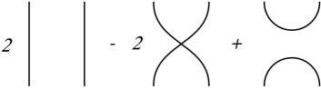
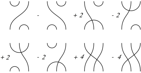
Figure 2: (a) The Hamiltonian (2.6). (b) The third charge (2.8).

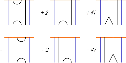
Figure 3: The result of application of the third charge to the defect state. The horizontal bar denotes the trace over the auxiliary space. The active sites are shown in thick black lines, while the spectator sites, unaffected by $Q$, are shown in blue.

Appendix A Action of third charge on defect state

In this appendix we prove eq. (2.12). This is most easily done graphically. The Hamiltonian density $H_{lm}$ and the third charge $Q_{lmn}$ are shown in fig. 2. Applying $Q_{l-1,l,l+1}$ to the defect state $\mathop{\mathrm{tr}}t_{i_{1}}\ldots t_{i_{L}}$, we get

$$(Q\cdot{\rm MPS})_{ijk} = \delta_{kj}t_{s}t_{s}t_{i}-\delta_{ij}t_{k}t_{s}t_{s}+2\delta_{ik}t_{j}t_{s}t_{s}-2\delta_{ik}t_{s}t_{s}t_{j}$$

$$+2\delta_{ij}t_{s}t_{k}t_{s}-2\delta_{jk}t_{s}t_{i}t_{s}+4t_{k}t_{i}t_{j}-4t_{j}t_{k}t_{i},$$

where $i,j,k$ are indices on sites $l-1,l,l+1$ and we have suppressed the rest of the wavefunction unaffected by the operator. Using the commutation relations (2.4) this can be brought to the form

$$(Q\cdot{\rm MPS})_{ijk}=\delta_{ij}t_{s}t_{s}t_{k}+2\delta_{ij}t_{k}+4i\varepsilon_{ijs}t_{s}t_{k}-\delta_{jk}t_{i}t_{s}t_{s}-2\delta_{jk}t_{i}-4it_{i}\varepsilon_{jks}t_{s},$$

depicted in fig. 3. The total charge vanishes upon summation over $l$, which should be clear from the figure.

References

- [1] O. DeWolfe, D. Z. Freedman and H. Ooguri, “Holography and defect conformal field theories”, Phys.Rev. D66, 025009 (2002), hep-th/0111135.
- [2] A. Karch and L. Randall, “Open and closed string interpretation of SUSY CFT’s on branes with boundaries”, JHEP 0106, 063 (2001), hep-th/0105132.
- [3] K. Nagasaki and S. Yamaguchi, “Expectation values of chiral primary operators in holographic interface CFT”, Phys.Rev. D86, 086004 (2012), 1205.1674.
- [4] C. Kristjansen, G. W. Semenoff and D. Young, “Chiral primary one-point functions in the D3-D7 defect conformal field theory”, JHEP 1301, 117 (2013), 1210.7015.
- [5] W. Nahm, “A Simple Formalism for the BPS Monopole”, Phys.Lett. B90, 413 (1980).
- [6] D.-E. Diaconescu, “D-branes, monopoles and Nahm equations”, Nucl.Phys. B503, 220 (1997), hep-th/9608163.
- [7] A. Giveon and D. Kutasov, “Brane dynamics and gauge theory”, Rev.Mod.Phys. 71, 983 (1999), hep-th/9802067.
- [8] N. R. Constable, R. C. Myers and O. Tafjord, “The Noncommutative bion core”, Phys.Rev. D61, 106009 (2000), hep-th/9911136.
- [9] J. A. Minahan and K. Zarembo, “The Bethe-ansatz for 4 super Yang-Mills”, JHEP 0303, 013 (2003), hep-th/0212208.
- [10] O. DeWolfe and N. Mann, “Integrable open spin chains in defect conformal field theory”, JHEP 0404, 035 (2004), hep-th/0401041.
- [11] A. Klümper, A. Schadschneider and J. Zittartz, “Equivalence and solution of anisotropic spin-1 models and generalized tJ fermion models in one dimension”, J. Phys. A 24, L955 (1991).
- [12] A. Klümper, A. Schadschneider and J. Zittartz, “Matrix product ground states for one-dimensional spin-1 quantum antiferromagnets”, Europhys. Lett. 24, 293 (1993).
- [13] L. Accardi, “Topics in quantum probability”, Phys. Rept. 77, 169 (1981).
- [14] M. Fannes, B. Nachtergaele and R. Werner, “Exact antiferromagnetic ground states of quantum spin chains”, Europhys. Lett. 10, 633 (1989).
- [15] M. Fannes, B. Nachtergaele and R. F. Werner, “Finitely correlated states on quantum spin chains”, Comm. Math. Phys. 144, 443 (1992).
- [16] S. Östlund and S. Rommer, “Thermodynamic limit of density matrix renormalization”, Phys. Rev. Lett. 75, 3537 (1995).
- [17] S. Rommer and S. Östlund, “Class of ansatz wave functions for one-dimensional spin systems and their relation to the density matrix renormalization group”, Phys. Rev. B55, 2164 (1997).
- [18] F. C. Alcaraz and M. J. Lazo, “Exact solutions of exactly integrable quantum chains by a matrix product ansatz”, J.Phys. A37, 4149 (2004), cond-mat/0312373.
- [19] F. Alcaraz and M. Lazo, “Generalization of the matrix product ansatz for integrable chains”, J.Phys. A39, 11335 (2006), cond-mat/0608177.
- [20] F. Verstraete, V. Murg and J. Cirac, “Matrix product states, projected entangled pair states, and variational renormalization group methods for quantum spin systems”, Adv. Phys. 57, 143 (2008).
- [21] H. Katsura and I. Maruyama, “Derivation of Matrix Product Ansatz for the Heisenberg Chain from Algebraic Bethe Ansatz”, J.Phys. A43, 175003 (2010), 0911.4215.
- [22] L. D. Faddeev, “How Algebraic Bethe Ansatz works for integrable model”, hep-th/9605187.
- [23] V. E. Korepin, N. M. Bogolyubov and A. G. Izergin, “Quantum inverse scattering method and correlation functions”, Cambridge Univ. Press (1993).
- [24] N. A. Slavnov, “The algebraic Bethe ansatz and quantum integrable systems”, Rus. Math. Surv. 62, 727 (2007).
- [25] M. Gaudin, “Diagonalisation d’une Classe d’Hamiltoniens de Spin”, J.Phys. France 37, 1087 (1976).
- [26] V. Korepin, “Calculation of norms of Bethe wave functions”, Commun.Math.Phys. 86, 391 (1982).
- [27] N. Slavnov, “Calculation of scalar products of wave functions and form factors in the framework of the algebraic Bethe ansatz”, Theor.Math.Phys. 79, 502 (1989).
- [28] B. Pozsgay, “Overlaps between eigenstates of the XXZ spin-1/2 chain and a class of simple product states”, 1309.4593.
- [29] M. Brockmann, J. De Nardis, B. Wouters and J.-S. Caux, “A Gaudin-like determinant for overlaps of Néel and XXZ Bethe States”, J. Phys. A: Math. Theor. 47, 145003 (2014), 1401.2877.
- [30] M. Brockmann, J. De Nardis, B. Wouters and J.-S. Caux, “Néel-XXZ state overlaps: odd particle numbers and Lieb-Liniger scaling limit”, J. Phys. A: Math. Theor. 47, 345003 (2014), 1403.7469.
- [31] J. Escobedo, N. Gromov, A. Sever and P. Vieira, “Tailoring Three-Point Functions and Integrability”, JHEP 1109, 028 (2011), 1012.2475.
- [32] J. Escobedo, N. Gromov, A. Sever and P. Vieira, “Tailoring Three-Point Functions and Integrability II. Weak/strong coupling match”, JHEP 1109, 029 (2011), 1104.5501.
- [33] N. Gromov, A. Sever and P. Vieira, “Tailoring Three-Point Functions and Integrability III. Classical Tunneling”, JHEP 1207, 044 (2012), 1111.2349.
- [34] N. Gromov and P. Vieira, “Quantum Integrability for Three-Point Functions of Maximally Supersymmetric Yang-Mills Theory”, Phys.Rev.Lett. 111, 211601 (2013), 1202.4103.
- [35] N. Gromov and P. Vieira, “Tailoring Three-Point Functions and Integrability IV. Theta-morphism”, JHEP 1404, 068 (2014), 1205.5288.
- [36] O. Foda, Y. Jiang, I. Kostov and D. Serban, “A tree-level 3-point function in the su(3)-sector of planar N=4 SYM”, JHEP 1310, 138 (2013), 1302.3539.
- [37] Y. Kazama, S. Komatsu and T. Nishimura, “A new integral representation for the scalar products of Bethe states for the XXX spin chain”, JHEP 1309, 013 (2013), 1304.5011.
- [38] Y. Jiang, I. Kostov, F. Loebbert and D. Serban, “Fixing the Quantum Three-Point Function”, JHEP 1404, 019 (2014), 1401.0384.
- [39] J. Caetano and T. Fleury, “Three-point functions and spin chains”, JHEP 1409, 173 (2014), 1404.4128.
- [40] Y. Kazama, S. Komatsu and T. Nishimura, “Novel construction and the monodromy relation for three-point functions at weak coupling”, JHEP 1501, 095 (2015), 1410.8533.
- [41] Y. Jiang, I. Kostov, A. Petrovskii and D. Serban, “String Bits and the Spin Vertex”, Nucl.Phys. B897, 374 (2015), 1410.8860.
- [42] B. Basso, S. Komatsu and P. Vieira, “Structure Constants and Integrable Bootstrap in Planar N=4 SYM Theory”, 1505.06745.
- [43] Y. Kazama, S. Komatsu and T. Nishimura, “On the singlet projector and the monodromy relation for spin chains and reduction to subsectors”, 1506.03203.
- [44] O. Foda, “ SYM structure constants as determinants”, JHEP 1203, 096 (2012), 1111.4663.
- [45] O. Foda and M. Wheeler, “Slavnov determinants, Yang-Mills structure constants, and discrete KP”, 1203.5621.
- [46] O. Foda and M. Wheeler, “Partial domain wall partition functions”, JHEP 1207, 186 (2012), 1205.4400.
- [47] O. Foda and M. Wheeler, “Variations on Slavnov’s scalar product”, JHEP 1210, 096 (2012), 1207.6871.
- [48] I. Kostov and Y. Matsuo, “Inner products of Bethe states as partial domain wall partition functions”, JHEP 1210, 168 (2012), 1207.2562.
- [49] I. Kostov, “Three-point function of semiclassical states at weak coupling”, J.Phys. A45, 494018 (2012), 1205.4412.
- [50] I. Kostov, “Classical Limit of the Three-Point Function of N=4 Supersymmetric Yang-Mills Theory from Integrability”, Phys.Rev.Lett. 108, 261604 (2012), 1203.6180.
- [51] E. Bettelheim and I. Kostov, “Semi-classical analysis of the inner product of Bethe states”, J.Phys. A47, 245401 (2014), 1403.0358.
- [52] I. Kostov, “Semi-classical scalar products in the generalised SU(2) model”, 1404.0235.
- [53] H. Bethe, “On the theory of metals. 1. Eigenvalues and eigenfunctions for the linear atomic chain”, Z.Phys. 71, 205 (1931).
- [54] Karbach, M and Müller, G, “Introduction to the Bethe ansatz I”, Comp. in Phys. 11, 36 (1998), cond-mat/9809162.
- [55] N. Beisert, C. Kristjansen and M. Staudacher, “The dilatation operator of 4 conformal super Yang-Mills theory”, Nucl. Phys. B664, 131 (2003), hep-th/0303060.
- [56] B. Sutherland, “Low-Lying Eigenstates of the One-Dimensional Heisenberg Ferromagnet for any Magnetization and Momentum”, Phys. Rev. Lett. 74, 816 (1995).
- [57] A. Dhar and B. S. Shastry, “Bloch Walls and Macroscopic String States in Bethe’s Solution of the Heisenberg Ferromagnetic Linear Chain”, Phys. Rev. Lett. 85, 2813 (2000).
- [58] N. Beisert, J. A. Minahan, M. Staudacher and K. Zarembo, “Stringing spins and spinning strings”, JHEP 0309, 010 (2003), hep-th/0306139.
- [59] S. Frolov and A. A. Tseytlin, “Rotating string solutions: AdS/CFT duality in non- supersymmetric sectors”, Phys. Lett. B570, 96 (2003), hep-th/0306143.
- [60] V. A. Kazakov, A. Marshakov, J. A. Minahan and K. Zarembo, “Classical/quantum integrability in AdS/CFT”, JHEP 0405, 024 (2004), hep-th/0402207.
- [61] A. Bissi, C. Kristjansen, D. Young and K. Zoubos, “Holographic three-point functions of giant gravitons”, JHEP 1106, 085 (2011), 1103.4079.
- [62] D. E. Berenstein, R. Corrado, W. Fischler and J. M. Maldacena, “The operator product expansion for Wilson loops and surfaces in the large N limit”, Phys. Rev. D59, 105023 (1999), hep-th/9809188.
- [63] K. Zarembo, “Holographic three-point functions of semiclassical states”, JHEP 1009, 030 (2010), 1008.1059.
- [64] M. S. Costa, R. Monteiro, J. E. Santos and D. Zoakos, “On three-point correlation functions in the gauge/gravity duality”, JHEP 1011, 141 (2010), 1008.1070.
- [65] M. Spradlin and A. Volovich, “Dressing the Giant Magnon”, JHEP 0610, 012 (2006), hep-th/0607009.
- [66] J. Gomis, T. Okuda and D. Trancanelli, “Quantum ’t Hooft operators and S-duality in N=4 super Yang-Mills”, Adv.Theor.Math.Phys. 13, 1941 (2009), 0904.4486.
- [67] S. Gukov and E. Witten, “Gauge Theory, Ramification, And The Geometric Langlands Program”, hep-th/0612073.
- [68] N. Drukker, J. Gomis and S. Matsuura, “Probing N=4 SYM With Surface Operators”, JHEP 0810, 048 (2008), 0805.4199.
- [69] A. Kapustin and S. Sethi, “The Higgs branch of impurity theories”, Adv.Theor.Math.Phys. 2, 571 (1998), hep-th/9804027.
- [70] D. Gaiotto and E. Witten, “Supersymmetric Boundary Conditions in N=4 Super Yang-Mills Theory”, J.Statist.Phys. 135, 789 (2009), 0804.2902.