Implementation of discretized Gabor frames and their duals

Abstract

The usefulness of Gabor frames depends on the easy computability of a suitable dual window. This question is addressed under several aspects: several versions of Schulz’s iterative algorithm for the approximation of the canonical dual window are analyzed for their numerical stability. For Gabor frames with totally positive windows or with exponential B-splines a direct algorithm yields a family of exact dual windows with compact support. It is shown that these dual windows converge exponentially fast to the canonical dual window.

Introduction

The discrete Gabor transform is a useful tool for the analysis and synthesis of nonstationary signals. It is based on the representation of the energy distribution of a signal in the time-frequency plane. Its applications range over the decomposition of musical and acoustical signals [1], [2], wireless communication [3], [4] and to the analysis of EEG signals [5], [6]. For a given window function $g\in L^{2}(\mathbb{R})$ and lattice parameters $\alpha,\beta>0$, the system of all corresponding time-frequency shifts

$$\mathcal{G}(g,\alpha,\beta)=\{M_{l\beta}\,T_{k\alpha}\,g=e^{2\pi il\beta\cdot}\,g(\cdot-k\alpha)\mid k,l\in\mathbb{Z}\}$$

is called a Gabor system for $L^{2}(\mathbb{R})$. It is called a Gabor frame for $L^{2}(\mathbb{R})$, if there exist constants $A,B>0$, such that

$$A\|f\|^{2}\leq\sum_{k,l\in\mathbb{Z}}|\langle f,M_{l\beta}T_{k\alpha}g\rangle|^{2}\leq B\|f\|^{2},\quad\forall f\in L^{2}(\mathbb{R}).$$ (1)

The constants $A,B$ are called lower and upper frame bounds of $\mathcal{G}(g,\alpha,\beta)$. If $\mathcal{G}(g,\alpha,\beta)$ fulfills only the right hand inequality, it is called a Bessel sequence and $B$ a Bessel bound. It is known that the frame inequality (1) implies the existence of a dual Gabor frame $\mathcal{G}(\gamma,\alpha,\beta)$ with dual window $\gamma\in L^{2}(\mathbb{R})$, such that every $f\in L^{2}(\mathbb{R})$ can be represented as

$$f=\sum_{k,l\in\mathbb{Z}}\langle f,M_{l\beta}T_{k\alpha}g\rangle\,M_{l\beta}T_{k\alpha}\gamma.$$ (2)

For a given Gabor system, the Gabor transform of a signal $f$ is defined as the analysis operator

$$\mathcal{C}_{g}:L^{2}(\mathbb{R})\rightarrow\ell^{2}(\mathbb{Z}^{2}),$$

$$\mathcal{C}_{g}f=(\langle f,M_{l\beta}T_{k\alpha}g\rangle)_{k,l\in\mathbb{Z}}.$$

The coefficient $\langle f,M_{l\beta}T_{k\alpha}g\rangle$ represents the energy distribution of $f$ near the point $(k\alpha,l\beta)$ in the time-frequency plane. It may also be interpreted as the amplitude of the frequency $l\beta$ at time $k\alpha$, insofar as such an interpretation is compatible with the uncertainty principle. The associated synthesis operator for the reconstructions (2) is the adjoint operator $\mathcal{C}_{g}^{*}$, and the frame operator $\mathcal{S}_{g}:L^{2}(\mathbb{R})\rightarrow L^{2}(\mathbb{R})$ is defined by

$$\mathcal{S}_{g}f=\mathcal{C}_{g}^{*}\,\mathcal{C}_{g}f=\sum_{k,l\in\mathbb{Z}}\langle f,M_{l\beta}T_{k\alpha}g\rangle\,M_{l\beta}T_{k\alpha}g.$$

In general, there exist many dual windows suitable for the reconstruction (2). The standard choice is the canonical dual window $\gamma^{\circ}=\mathcal{S}_{g}^{-1}g$. For a characterization of all dual windows see [7, 8]. Since the applicability and usefulness of Gabor frames depends heavily on the knowledge and computability of a dual window, the numerical construction of dual windows has motivated numerous studies. As representative contributions we mention  [9, 10] and the large time-frequency analysis toolbox (LTFAT) [11].

Our contribution to the analysis of dual Gabor windows is twofold. On a general level, we study numerically stable methods for the computation of the canonical dual window $\gamma^{\circ}=\mathcal{S}_{g}^{-1}g$. On a specific level, we study the efficient construction and the behavior of a sequence of dual windows for Gabor frames with totally positive window functions and with exponential B-splines.

We first present two stable implementations of a conventional iterative algorithm to approximate $\gamma^{\circ}$. The algorithm was originally proposed by Schulz [12] for matrix inversion. It is based on the Neumann series for the inverse frame operator and converges quadratically, see Algorithm 2. We provide a detailed analysis of the numerical error and show that our two implementations (the operator version and the first vector version) are stable. By contrast, the implementation proposed by Janssen (see [13] and [14]) is often unstable because the numerical error roughly doubles in each step. Therefore the first two implementations are much preferable. As two illustrative examples, we use the window functions MONSTER defined in [9] and a Gaussian window $g$, in order to compare all three implementations. The numerical results agree precisely with the predicted behavior of the numerical error.

We then describe recent results on special Gabor systems whose window function is a totally positive (TP) function of finite type or an exponential B-spline (EB-spline). TP functions are remarkable because so far they are the only window functions for which a complete characterization of all lattice parameters such that $\mathcal{G}(g,\alpha,\beta)$ is a frame is known. More precisely, the Gabor system $\mathcal{G}(g,\alpha,\beta)$, with a TP function $g$ of finite type $N\geq 2$ is a frame if and only if $\alpha\beta<1$ [15]. Subsequently, similar arguments in [16] showed that the Gabor system $\mathcal{G}(B_{\Lambda},\alpha,\beta)$ of an EB-spline constitutes a frame for $\alpha=1$, $\beta<1$, and some other lattice parameters, too. The proofs also provide a constructive method for the computation of infinitely many dual windows $\gamma_{L}$ with compact support, which we summarize in Algorithm 5 for TP functions of finite type and Algorithm 7 for EB-splines.

This construction offers several new and useful aspects that are special for TP windows and not shared by general window functions.

(i) Algorithms 5 and  7 provide a family of dual windows $\gamma_{L}$ both in finite and infinite dimensional models, namely for continuous signals in $L^{2}(\mathbb{R})$, for discrete signals in $\ell^{2}(\mathbb{Z})$, and for periodic discrete signals in $\mathbb{C}^{N}$. Currently available toolboxes, such as LTFAT [11], work only for finite-dimensional signals.

(ii) The dual windows $\gamma_{L}$ possess compact support of size $\mathcal{O}(L)$, whereas the canonical dual $\gamma^{\circ}$ is known to have infinite support.

(iii) The dual windows $\gamma_{L}$ are exact and satisfy (2). This is in contrast to the standard iterative methods for the approximation of the canonical dual (see e.g. Algorithm 2), which generate only approximations of a dual window.

As our main mathematical result we prove that the dual windows $\gamma_{L}$ are good approximations of the canonical dual window $\gamma^{\circ}=\mathcal{S}_{g}^{-1}g$ and we show that they converge exponentially fast to the canonical dual window, i.e., $\|\gamma_{L}-\gamma^{\circ}\|_{2}=\mathcal{O}(e^{-\rho L})$. Therefore, by specifying the parameter $L$, Algorithms 5 and 7 provide a dual window $\gamma_{L}$ with compact support and which approximates the canonical dual at a desired rate.

The proof uses some ideas of the non-symmetric finite section method, but also requires a new technique related to the formulation of the Moore-Penrose pseudo-inverse of infinite matrices in terms of orthogonal projections.

As our main numerical contribution, we study and implement the case of discrete Gabor frames. We present some fast and stable algorithms to evaluate and discretize TP functions and EB-splines and their dual windows computed by the Algorithms 5 and 7. These algorithms are proposed as extensions to the Large Time Frequency Analysis Toolbox described in [11].

The paper is organized as follows: In section I we study the numerical stability of a fast iterative algorithm for the approximation of the canonical dual window. In section II we summarize the algorithms for the construction of dual windows of TP functions and EB splines. In section III we formulate and discuss the main theorems about the convergence of the compactly supported dual windows $\gamma_{L}$ to the canonical dual window $\gamma^{\circ}$. Section IV explains some details about the implementation of Gabor frames with TP functions and EB splines. The appendix contains the technical details of the proofs of the main results.

I Some iterative algorithms for approximating the canonical dual

In this section we describe two iterative algorithms for approximating the canonical dual of an arbitrary frame $\mathcal{F}=\{f_{j}\}_{j\in I}$ for a Hilbert space $\mathcal{H}$. The central part of such algorithms is the approximation of the inverse of the corresponding frame operator

$$S_{\mathcal{F}}:\mathcal{H}\to\mathcal{H},\qquad S_{\mathcal{F}}h=\sum_{j\in I}\langle h,f_{j}\rangle f_{j}.$$

We discuss the convergence and the numerical stability of various implementations. Finally we present some numerical tests. The following approximation schemes are proposed in the literature.

Algorithm 1 (Frame algorithm).

Choose $0<\lambda<2/B$, with $B$ the upper frame bound of $\mathcal{F}$. Then $q:=\lVert I-\lambda\,S_{\mathcal{F}}\rVert<1$ and

$$S_{\mathcal{F}}^{-1}=\lambda\,\sum_{n=0}^{\infty}(I-\lambda\,S_{\mathcal{F}})^{n}.$$

The partial sums of this Neumann series can be computed iteratively by

$$K_{0}=\lambda\,I,$$

$$K_{k+1}=\lambda\,I+(I-\lambda\,S_{\mathcal{F}})\,K_{k},\ \ k\in\mathbb{N}_{0}.$$ (3)

The convergence rate is of order $\lVert S_{\mathcal{F}}^{-1}-K_{k}\rVert=\mathcal{O}(q^{k})$. The $k$’th approximation of the canonical dual frame $\mathcal{F}^{\circ}=\{S_{\mathcal{F}}^{-1}\,f_{j}\}_{j\in I}$ is given by $\{K_{k}\,f_{j}\}_{j\in I}$.

This algorithm is very robust, but slow if $q$ is close to one. This algorithm can be accelerated [17] with conjugate gradient techniques and with a convergence rate $\big{(}\frac{\sqrt{B}-\sqrt{A}}{\sqrt{B}+\sqrt{A}}\big{)}^{k}$ after $k$ iterations regardless of whether the frame bounds $A,B$ are known or not.

An even faster method goes back to Schulz [12] and Hotelling [18].

Algorithm 2 (Schulz iteration).

Choose $0<\lambda<2/B$. The version of Schulz iteration with ”initial scaling” [14, Algorithm IV] is

$$J_{0}=\lambda\,I,$$

$$J_{k+1}=2\,J_{k}-J_{k}\,S_{\mathcal{F}}\,J_{k},\ \ k\in\mathbb{N}_{0}.$$ (4)

This iteration implies the identity $J_{k}=K_{2^{k}-1}$ and is therefore connected to the frame algorithm. The Schulz algorithm converges quadratically, i.e.

$$\lVert S_{\mathcal{F}}^{-1}-J_{k+1}\rVert\leq\lVert S_{\mathcal{F}}\rVert\,\lVert S_{\mathcal{F}}^{-1}-J_{k}\rVert^{2}=\mathcal{O}(q^{2^{k+1}}).$$ (5)

This algorithm was first described by Schulz [12] who used this method for matrix inversion.

Proof:

The claims in Algorithm 2 are proved by induction. Since Schulz’s algorithm is not as known as other iterative algorithms, we sketch the main steps. We first show that

$$I-S_{\mathcal{F}}J_{k}=I-J_{k}S_{\mathcal{F}}=(I-\lambda S_{\mathcal{F}})^{2^{k}}\,.$$ (6)

Assuming that (6) is correct for $k\in\mathbb{N}_{0}$, we obtain

$$I-S_{\mathcal{F}}J_{k+1} =I-S_{\mathcal{F}}(2J_{k}-J_{k}S_{\mathcal{F}}J_{k})$$

$$=(I-S_{\mathcal{F}}J_{k})^{2}=\Big{(}(I-\lambda S_{\mathcal{F}})^{2^{k}}\Big{)}^{2}\,,$$

as claimed. Using (6), we show again by induction that $J_{k}=K_{2^{k}-1}=\lambda\sum_{j=0}^{2^{k}-1}(I-\lambda S_{\mathcal{F}})^{j}$:

$$\lambda \sum_{j=0}^{2^{k+1}-1}(I-\lambda S_{\mathcal{F}})^{j}$$

$$=\lambda\sum_{j=0}^{2^{k}-1}(I-\lambda S_{\mathcal{F}})^{j}+(I-\lambda S_{\mathcal{F}})^{2^{k}}\,\lambda\sum_{j=0}^{2^{k}-1}(I-\lambda S_{\mathcal{F}})^{j}$$

$$=J_{k}+(I-J_{k}S_{\mathcal{F}})J_{k}=J_{k+1}\,.$$

The quadratic convergence rate now follows from the convergence properties of the Neumann series. ∎

We discuss the implementation of Algorithm 2 in the case of a Gabor frame $\mathcal{G}(g,\alpha,\beta)$. Recall that the canonical dual frame is determined by the dual window $\gamma^{\circ}=\mathcal{S}_{g}^{-1}g$. We compare three different implementations of the Schulz iteration and provide some heuristics for their numerical stability.

(i) Operator form: The numerical computation of the Schulz iteration as stated in Algorithm 2 provides operators $\hat{J}_{k}=J_{k}+E_{k}$, where $E_{k}$ denotes the accumulated forward error. Let $Y_{k+1}$ denote the new roundoff error in the $k+1$’st iteration, then the operator after $k+1$ iterations of (4) is

$$\hat{J}_{k+1} =2\,\hat{J}_{k}-\hat{J}_{k}\,\mathcal{S}_{g}\,\hat{J}_{k}+Y_{k+1}$$

$$=J_{k+1}+E_{k}\,(I-\mathcal{S}_{g}\,J_{k})+(I-J_{k}\,\mathcal{S}_{g})\,E_{k}+Y_{k+1}+\mathcal{O}(\lVert E_{k}\rVert^{2}).$$

Since $I-\mathcal{S}_{g}\,J_{k}=I-J_{k}\,\mathcal{S}_{g}=(I-\lambda\,\mathcal{S}_{g})^{2^{k}}$, we have

$$\lVert E_{k+1}\rVert=\lVert\hat{J}_{k+1}-J_{k+1}\rVert\leq 2\,q^{2^{k}}\,\lVert E_{k}\rVert+\lVert Y_{k+1}\rVert+\mathcal{O}(\lVert E_{k}\rVert^{2}).$$

This estimate shows that the error accumulated in the first $k$ iterations is damped and only a new round-off error is added. Hence this iteration is numerically stable.

(ii) Vector form: We compute approximations of the dual window $\gamma^{\circ}$ directly by setting $\gamma_{k}:=J_{k}\,g$ with the following algorithm:

$$\gamma_{0}=\lambda\,g$$

$$\gamma_{k+1}=2\,\gamma_{k}-\mathcal{C}^{*}_{\gamma_{k}}\,\mathcal{C}_{g}\,\gamma_{k},\ \ k\in\mathbb{N}_{0}\,.$$ (7)

Proof:

We use the fact that $S_{\mathcal{F}}$ and thus all $J_{k}$ commute with the time-frequency shifts $M_{l\beta}T_{j\alpha}$. This commutation rule implies the identity

$$\mathcal{C}_{\gamma_{k}}^{*}\,\boldsymbol{c}=\sum_{j,l\in\mathbb{Z}}c_{j,l}\,J_{k}\,M_{l\beta}\,T_{j\alpha}\,g=J_{k}\,\mathcal{C}_{g}^{*}\,\boldsymbol{c}$$

for all $\boldsymbol{c}\in\ell^{2}(\mathbb{Z}^{2})$. Consequently

$$\gamma_{k+1} =J_{k+1}g=2J_{k}g-J_{k}\mathcal{S}_{g}J_{k}g$$

$$=2\gamma_{k}-J_{k}\mathcal{C}^{*}_{g}\mathcal{C}_{g}\gamma_{k}=2\gamma_{k}-\mathcal{C}^{*}_{\gamma_{k}}C_{g}\gamma_{k}\,.$$

∎

The numerical computation yields $\hat{\gamma}_{k}=\gamma_{k}+e_{k}$, where $e_{k}$ denotes the accumulated forward error. Let $y_{k+1}$ denote the new roundoff error, then in the $k+1$’th step of the iteration (7) we have

$$\hat{\gamma}_{k+1} =2\,\hat{\gamma}_{k}-\mathcal{C}^{*}_{\hat{\gamma}_{k}}\,\mathcal{C}_{g}\,\hat{\gamma}_{k}+y_{k+1}$$

$$=\gamma_{k+1}+(e_{k}-\mathcal{C}_{\gamma_{k}}^{*}\,\mathcal{C}_{g}\,e_{k})+(e_{k}-\mathcal{C}_{e_{k}}^{*}\,\mathcal{C}_{g}\,\gamma_{k})+y_{k+1}+\mathcal{O}(\lVert e_{k}\rVert_{2}^{2})\,.$$

The aforementioned estimates give

$$\lVert(I-\mathcal{C}_{\gamma_{k}}^{*}\,\mathcal{C}_{g})\,e_{k}\rVert_{2}=\lVert(I-J_{k}\,\mathcal{S}_{g})\,e_{k}\rVert_{2}\leq q^{2^{k}}\,\lVert e_{k}\rVert_{2}.$$

Moreover the Janssen representation (see [8, p.131]) gives

$$\mathcal{C}_{e_{k}}^{*}\,\mathcal{C}_{g}\,\gamma_{k}=\frac{1}{\alpha\beta}\sum_{j,l\in\mathbb{Z}}\langle e_{k},M_{j/\alpha}\,T_{l/\beta}\,g\rangle M_{j/\alpha}\,T_{l/\beta}\,\gamma_{k}.$$

The last expression, when $\gamma_{k}$ is replaced by $\gamma^{\circ}$, is the orthogonal projection $\Pi_{V_{g}}e_{k}$ of $e_{k}$ onto $V_{g}:=\overline{\mathrm{span}}\bigl{(}\mathcal{G}(g,1/\beta,1/\alpha)\bigr{)}$ and therefore

$$\lVert e_{k}-\mathcal{C}_{e_{k}}^{*}\,\mathcal{C}_{g}\,\gamma^{\circ}\rVert_{2}\leq\lVert e_{k}\rVert_{2}$$

and

$$\lVert e_{k} -\mathcal{C}_{e_{k}}^{*}\,\mathcal{C}_{g}\,\gamma_{k}\rVert_{2}\leq\lVert e_{k}-\mathcal{C}_{e_{k}}^{*}\,\mathcal{C}_{g}\,\gamma^{\circ}\rVert_{2}+\lVert C_{e_{k}}^{*}\,\mathcal{C}_{g}\,(\gamma^{\circ}-\gamma_{k})\rVert_{2}\leq\lVert e_{k}\rVert_{2}+\mathcal{O}(q^{2^{k}})\,.$$

Since $\lVert\gamma^{\circ}-\gamma_{k}\rVert_{2}=\mathcal{O}(q^{2^{k}})$ by (5), the new numerical error is

$$\lVert e_{k+1}\rVert_{2}\leq(1+q^{2^{k}})\lVert e_{k}\rVert_{2}+\lVert y_{k+1}\rVert_{2}+\mathcal{O}(\lVert e_{k}\rVert^{2}_{2}+q^{2^{k}})\,.$$

In contrast to the operator version, $\lVert e_{k}\rVert_{2}$ enters linearly with coefficient $\approx 1$. Thus the numerical stability is plausible and is also confirmed by our numerical results in Example 3.

(iii) Janssen’s alternative vector version: Janssen [14, Algorithm IV] proposes the approximations

$$\gamma_{0}=\lambda\,g,$$

$$\gamma_{k+1}=2\,\gamma_{k}-\mathcal{C}^{*}_{\gamma_{k}}\,\mathcal{C}_{\gamma_{k}}\,g,\ \ k\in\mathbb{N}_{0}.$$ (8)

However, in their numerical tests of (8) Janssen and Søndergaard [9] observed some numerical instability. With notations as in (ii), the numerical error in step $k+1$ is

$$e_{k+1} =\hat{\gamma}_{k+1}-\gamma_{k+1}$$

$$=2\,e_{k}-\mathcal{C}_{\gamma_{k}}^{*}\,\mathcal{C}_{e_{k}}\,g-\mathcal{C}_{e_{k}}^{*}\,\mathcal{C}_{\gamma_{k}}\,g+y_{k+1}+\mathcal{O}(\lVert e_{k}\rVert_{2}^{2}).$$

We show that the error may grow by at least a factor of $2$ in each step. Note that $V_{g}$ in (ii) is a proper subset of $L^{2}(\mathbb{R})$, if $\alpha\beta<1$. Hence $\lVert(I-\Pi_{V_{g}})\,e_{1}\rVert_{2}\approx\varepsilon$, where $\varepsilon$ denotes the machine accuracy. The Janssen representation implies, that $\mathcal{C}_{\gamma_{k}}^{*}\,\mathcal{C}_{e_{k}}\,g$ and $\mathcal{C}_{e_{k}}^{*}\,\mathcal{C}_{\gamma_{k}}\,g$ are in $V_{g}$. Therefore,

$$(I-\Pi_{V_{g}})\,e_{k+1}=2\,(I-\Pi_{V_{g}})\,e_{k} +(I-\Pi_{V_{g}})\,y_{k+1}+\mathcal{O}(\lVert e_{k}\rVert_{2}^{2})$$

This shows, that the error components in $V_{g}^{\perp}$ can double in each step. In Example 3 we demonstrate that this numerical instability may indeed occur.

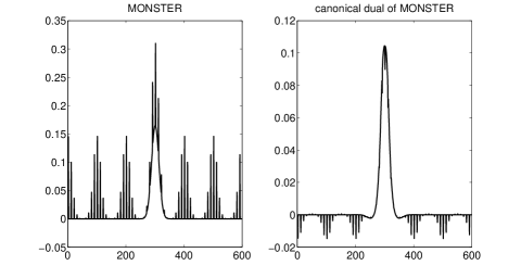
Figure 1: MONSTER function and its canonical dual for $\alpha=20$ and $\beta=1/50$, computed by a routine of LTFAT [11].

Example 3.

As it was described in (iii) the implementation (8) by Janssen can have some stability problems and should be applied carefully. We use the function MONSTER (see Figure 1) in [9] and $\alpha=20$, $\beta=1/50$ for our numerical tests of all three implementations of the Schulz iteration. As we can see in Figure 2, the operator version is stable, the vector version of (ii) is also useful, while the error of the implementation in (iii) explodes. The same conclusions hold for the window function $g(x)=e^{-\pi x^{2}/600}$ with $\alpha=20,\beta=1/50$, as is shown in Figure 3.

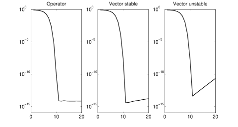
Figure 2: Error $\lVert\mathcal{C}_{\gamma^{\circ}}-\mathcal{C}_{\hat{\gamma}_{k}}\rVert$ of the three implementations of Algorithm 2 for $20$ iteration steps to approximate the canonical dual window of MONSTER for $\alpha=20$ and $\beta=1/50$.

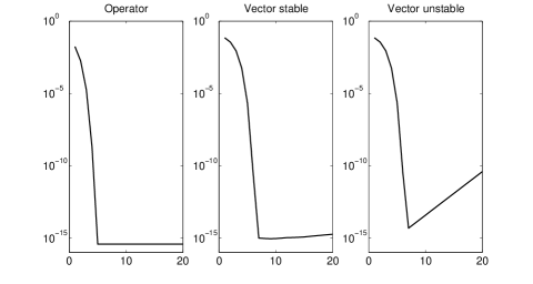
Figure 3: $\lVert\mathcal{C}_{\gamma^{\circ}}-\mathcal{C}_{\hat{\gamma}_{k}}\rVert$ of the three implementations of Algorithm 2 for $20$ iteration steps to approximate the canonical dual window of the Gaussian $g(x)=e^{-\pi x^{2}/600}$ for $\alpha=20$ and $\beta=1/50$.

II Gabor frames of totally positive functions and exponential B-splines

We now consider totally positive functions of finite type and exponential B-splines as window functions. The TP functions attracted much interest recently, as they provide new examples of window functions for which the necessary density condition $\alpha\beta<1$ of the lattice parameters is also sufficient [15]. For detailed information on total positivity of functions and matrices see [19], for a detailed introduction to exponential B-splines see [20] and [21].

Definition 4.

[22], [23] An integrable function $g:\mathbb{R}\rightarrow\mathbb{R}$ is called totally positive (TP), if its Fourier transform factors as

$$\hat{g}(\omega) =\int_{-\infty}^{\infty}g(t)e^{-2\pi it\omega}\,dt$$

$$=Ce^{-\eta\omega^{2}}e^{-2\pi i\delta\omega}\prod_{\nu=1}^{\infty}\frac{e^{2\pi i\delta_{\nu}\omega}}{1+2\pi i\delta_{\nu}\omega},$$ (9)

where $C,\eta,\delta,\delta_{\nu}$ are real parameters with

$$C>0,\ \ \eta\geq 0,\ 0<\eta+\sum_{\nu=1}^{\infty}\delta_{\nu}^{2}<\infty\,.$$

Note that in Schoenberg’s terminology there also exist TP functions that are not integrable. Therefore the given definition does not include the most general case of TP functions. Here we only consider TP functions $g_{\Delta}$ of finite type $N\in\mathbb{N}$, with $\eta=0$, $\Delta=(\delta_{1},\ldots,\delta_{N})$ and

$$\widehat{g_{\Delta}}(\omega)=\prod_{\nu=1}^{N}(1+2\pi i\delta_{\nu}\omega)^{-1}.$$ (10)

For $N=1$ and $\Delta=(\delta)$ we have the one-sided exponential

$$g_{\delta}(x)=\frac{1}{|\delta|}\,e^{-\delta^{-1}x}\,\chi_{(0,\infty)}(\delta x)\quad\hbox{for}\quad x\in\mathbb{R}\setminus\{0\},$$

with support $[0,\infty)$ for positive $\delta$ and $(-\infty,0]$ for negative $\delta$, and for $N>1$ and $\Delta=(\delta_{1},\ldots,\delta_{N})$, $g_{\Delta}$ is the $N$-fold convolution

$$g_{\Delta}=g_{\delta_{1}}\ast\cdots\ast g_{\delta_{N}}.$$

Especially, if $\delta_{\nu}=\delta\neq 0$ for all $1\leq\nu\leq N$, then

$$g_{\Delta}(x)=\frac{|x|^{N-1}}{|\delta|^{N}(N-1)!}\,e^{-\delta^{-1}x}\,\chi_{(0,\infty)}(\delta x).$$

The functions $g_{\Delta}$ are nonnegative, have infinite support, and exponential decay, precisely, if $\tau=(\max\{\,2\pi\,\lvert\delta_{\nu}\rvert\mid\nu=1,\ldots,N\})^{-1}$ and $\epsilon>0$, then there is a constant $c=c(\epsilon)$ such that

$$0\leq g_{\Delta}(x)\leq c\,e^{-(\tau-\varepsilon)\lvert x\rvert}.$$ (11)

Moreover, if $\delta_{1}\neq\delta_{N}$ and we specify $g_{\delta}(0)=1/|2\delta|$, the recurrence relation

$$g_{\delta_{1},\ldots,\delta_{N}}=\frac{\delta_{1}^{-1}g_{\delta_{2},\ldots,\delta_{N}}-\delta_{N}^{-1}g_{\delta_{1},\ldots,\delta_{N-1}}}{\delta_{1}^{-1}-\delta_{N}^{-1}}$$

holds. For later use, we denote by $m$ (resp. $n$) the number of positive (resp. negative) parameters $\delta_{\nu}$.

The main result in [15] shows that the Gabor system $\mathcal{G}(g,\alpha,\beta)$ of a TP function of finite type $m+n\geq 2$ constitutes a Gabor frame if and only if $\alpha\beta<1$. The proof provides an algorithm for the computation of a dual window $\gamma$ with compact support. This method was adapted in [24], [25] in order to supply infinitely many dual windows $\gamma_{L}$. The computation of $\gamma_{L}(x+j\alpha)$, with $j\in\mathbb{Z}$, is performed by computing a single row of a left-inverse of the biinfinite pre-Gramian matrix

$$P_{g}(x):=\left(\overline{g}\left(x+\alpha j-\tfrac{k}{\beta}\right)\right)_{j,k\in\mathbb{Z}}.$$ (12)

The structure of the left-inverse of $P_{g}(x)$ heavily depends on the property that $g$ is totally positive. We include the algorithm for the reader’s convenience.

Algorithm 5.

[24] Input parameters are the parameter vector $\Delta=(\delta_{1},\delta_{2},\dots,\delta_{N})$ of the window $g$, the lattice parameters $\alpha,\beta>0$ with $\alpha\beta<1$, a parameter $L\in\mathbb{N}_{0}$ controlling the support size of the dual window $\gamma_{L}$, and a point $x\in[0,\alpha)$.

Output parameters are integers $i_{1}(L),i_{2}(L)$ and the vector of values $\gamma_{L}(x+\alpha j)$, $i_{1}(L)\leq j\leq i_{2}(L)$, in the support of $\gamma_{L}$, such that $\gamma_{L}:\mathbb{R}\rightarrow\mathbb{R}$ defines a dual window of $g$.

1. Set $r:=\left\lfloor\frac{1}{1-\alpha\beta}\right\rfloor$, $k_{1}=-(r+1)m$ and $k_{2}=(r+1)n$.

2. Set $k_{1}(L):=k_{1}-L$ and $k_{2}(L):=k_{2}+L$,

   $$i_{1}(L) :=\left\lfloor\frac{k_{1}-L+m-1}{\alpha\beta}-\frac{x}{\alpha}\right\rfloor+1,$$

   $$i_{2}(L) :=\left\lceil\frac{k_{2}+L-n+1}{\alpha\beta}-\frac{x}{\alpha}\right\rceil-1.$$

3. Set $P_{L}(x):=(p_{j,k})_{i_{1}(L)\leq j\leq i_{2}(L),~{}k_{1}(L)\leq k\leq k_{2}(L)}$, where

   $$p_{j,k}=g\left(x+\alpha j-\frac{k}{\beta}\right).$$

4. Compute the pseudoinverse

   $$P_{L}(x)^{\dagger}=(q_{k,j})_{k_{1}(L)\leq k\leq k_{2}(L),~{}i_{1}(L)\leq j\leq i_{2}(L)}$$

   of $P_{L}(x)$.

5. Take the row with index $k=0$ of $P_{L}(x)^{\dagger}$. Its coefficients define the values of the dual window $\gamma_{L}$ at the points $\{x+\alpha j\,|\,i_{1}(L)\leq j\leq i_{2}(L)\}$, i.e.

   $$\gamma_{L}(x+\alpha j):=\begin{cases}\beta\,q_{0,j}&\text{, if }i_{1}(L)\leq j\leq i_{2}(L),\\ 0&\text{, if }j<i_{1}(L)~{}\text{or }j>i_{2}(L).\end{cases}$$ (13)

In particular, the support of the dual window $\gamma_{L}$ is contained in the interval $[\alpha i_{1}(L),\alpha(i_{2}(L)+1)]$ of length of the order $\beta^{-1}(k_{2}-k_{1}+2L)$. Thus the parameter $L$ labels the size of the support.

A related class of window functions is the class of exponential B-splines. These functions are positive and have compact support, a property which is desirable in some applications.

Definition 6.

For $\Lambda=(\lambda_{1},\ldots,\lambda_{N})\in\mathbb{R}^{N}$ the exponential B-spline (EB-spline) $B_{\Lambda}$ with knots $0,1,\ldots,N$ is given by its Fourier transform

$$\widehat{B_{\Lambda}}(\omega)=\prod_{\nu=1}^{N}\frac{e^{\lambda_{\nu}-2\pi i\omega}-1}{\lambda_{\nu}-2\pi i\omega}.$$ (14)

In [16], it was shown that the Gabor system $\mathcal{G}(B_{\Lambda},\alpha,\beta)$ of every EB-spline constitutes a frame for $\alpha=1$, $\beta<1$ (and also some other lattice parameters). Similar to the case of TP functions, the following algorithm provides dual windows $\gamma_{L}$ of the Gabor frame $\mathcal{G}(B_{\Lambda},\alpha,\beta)$.

Algorithm 7.

[16] Input parameters are the parameter vector $\Lambda\in\mathbb{R}^{N}$ of the window $B_{\Lambda}$, the lattice parameters $\alpha,\beta>0$, a parameter $L\in\mathbb{N}_{0}$ controlling the support size of the dual window $\gamma_{L}$, and a point $x\in\left[\frac{N-\alpha}{2},\frac{N+\alpha}{2}\right)$.

Output parameters are integers $i_{1}(L),i_{2}(L)$ and the vector of values $\gamma_{L}(x+\alpha j)$, $i_{1}(L)\leq j\leq i_{2}(L)$, in the support of $\gamma_{L}$, such that $\gamma_{L}:\mathbb{R}\rightarrow\mathbb{R}$ defines a dual window of $B_{\Lambda}$.

1. Set $k_{2}(L)=\left\lfloor\frac{N\beta+\alpha\beta}{2(1-\alpha\beta)}\right\rfloor+1+L$ and $k_{1}(L)=-k_{2}(L)$.

2. Set $i_{1}(L)\leq k_{1}(L)$ and $i_{2}(L)\geq k_{2}(L)$, such that

   $$B_{\Lambda}\left(x+(i_{1}(L)-1)\alpha-\tfrac{k_{1}(L)-1}{\beta}\right)\neq 0,$$

   $$B_{\Lambda}\left(x+i_{1}(L)\alpha-\tfrac{k_{1}(L)-1}{\beta}\right)=0,$$

   $$B_{\Lambda}\left(x+(i_{2}(L)+1)\alpha-\tfrac{k_{2}(L)+1}{\beta}\right)\neq 0,$$

   $$B_{\Lambda}\left(x+i_{2}(L)\alpha-\tfrac{k_{2}(L)+1}{\beta}\right)=0.$$

3. Set $P_{L}(x):=(p_{j,k})_{i_{1}(L)\leq j\leq i_{2}(L),~{}k_{1}(L)\leq k\leq k_{2}(L)}$, where

   $$p_{j,k}=B_{\Lambda}\left(x+\alpha j-\frac{k}{\beta}\right).$$

4. Compute the pseudoinverse

   $$P_{L}(x)^{\dagger}=(q_{k,j})_{k_{1}(L)\leq k\leq k_{2}(L),~{}i_{1}(L)\leq j\leq i_{2}(L)}$$

   of $P_{L}(x)$.

5. Take the row with index $k=0$ of $P_{L}(x)^{\dagger}$. Its coefficients define the values of the dual window $\gamma_{L}$ at the points $\{x+\alpha j\,|\,i_{1}(L)\leq j\leq i_{2}(L)\}$, i.e.

   $$\gamma_{L}(x+\alpha j):=\begin{cases}\beta\,q_{0,j}&\text{, if }i_{1}(L)\leq j\leq i_{2}(L),\\ 0&\text{, if }j<i_{1}(L)~{}\text{or }j>i_{2}(L).\end{cases}$$ (15)

We would like to emphasize the following point: (i) These algorithms determine the precise values of a dual window $\gamma$ with compact support in $L^{2}(\mathbb{R})$ and not just a discrete approximation in a finite-dimensional vector space, as is done in most existing algorithms in [11, 10].

(ii) Although the problem of finding a dual window is by nature infinite-dimensional in $L^{2}(\mathbb{R})$, the computation of $\gamma_{L}$ on a grid $\tfrac{\alpha}{M}\mathbb{Z}$ requires only the pseudo-inversion of $M$ finite-dimensional matrices.

III Approximation of the canonical dual of TP functions and EB-splines

We fix the parameters $\alpha,\beta>0$ of the Gabor frame and let $g$ be either a TP function of finite type with parameter set $\Delta$ or an EB-spline with parameter set $\Lambda$. The pre-Gramian matrix (12) plays a central role in the characterization of the frame bounds $A,B$ of the Gabor system $\mathcal{G}(g,\alpha,\beta)$, and in finding dual windows $\gamma$.

In this section we address the question how the sequence of dual windows $\gamma_{L}$ of Algorithms 5 and  7 are related to the canonical dual window $\gamma^{\circ}$. Our main goal is to prove that the compactly supported dual windows $\gamma_{L}$ computed by the Algorithms 5 and 7 from [24] and [16] approximate the canonical dual window $\gamma^{\circ}$ at a rate

$$\left\|\gamma_{L}-\gamma^{\circ}\right\|_{2}\leq\tilde{c}\,e^{-\rho L},$$

where $L$ determines the support of $\gamma_{L}$ and $\rho>0$.

As a first step we show that the norm of $\gamma_{L}$ remains bounded as $L$ tends to $\infty$.

Theorem 8.

Let $g$ be a TP function of finite type as defined by (10). Then there exist constants $A,B>0$ independent of $L\in\mathbb{N}_{0}$ such that

$$A\|\boldsymbol{c}\|_{2}\leq\|P_{L}(x)\boldsymbol{c}\|_{2}\leq B\|\boldsymbol{c}\|_{2}$$ (16)

for all $\boldsymbol{c}\in\mathbb{C}^{k_{2}(L)-k_{1}(L)+1}$ and $x\in[0,\alpha)$, where $P_{L}(x)$ is the finite section of the corresponding biinfinite pre-Gramian matrix $P_{g}(x)$ as described in Algorithm 5. Consequently, $\left\|\gamma_{L}\right\|_{2}\leq\sqrt{\alpha}\,\beta\,A^{-1}$, for all $L\in\mathbb{N}$.

The precise proof will be given in the appendix. The proof idea goes as follows: The upper bound $B$ is easily obtained from Schur’s test based on the exponential decay of $g$ in (11). For the lower bound $A$, we choose $2L+1$ submatrices $R_{\ell}$ of $P_{L}(x)$, with $k_{2}-k_{1}+1$ columns each, and build a left-inverse $Q_{L}(x)$ of $P_{L}(x)$ by the selection of specific rows of $R_{\ell}^{\dagger}$. The result in [15, Theorem 9] shows that all matrices $R_{\ell}^{\dagger}$ are bounded uniformly in $x$. Their upper bound $C$ will provide the upper bound $A^{-1}=C\,\tfrac{k_{2}-k_{1}+1}{\alpha\beta}$ for all matrices $Q_{L}(x)$ uniformly in $x$ and $L$. Hence $A$ is a suitable constant for the lower bound of $P_{L}(x)$.

To prove the rate of approximation of the dual windows $\gamma_{L}$, we recall that the canonical dual window $\gamma^{\circ}=\mathcal{S}_{g}^{-1}g$ can be expressed by the Moore-Penrose pseudoinverse of $P_{g}(x)$, namely

$$\gamma^{\circ}(x+\alpha j)=\beta\,(P_{g}(x)^{\dagger})_{0,j}$$ (17)

for all $j\in\mathbb{Z}$ and all $x\in[0,\alpha)$. This is a direct consequence of the Wexler-Raz criterion for the dual windows of $g$ [8, Theorem 7.3.1], and the minimal $L^{2}$-norm of the canonical dual among all duals of $g$ [26]. We will therefore show that the zeroth row of $P_{L}(x)^{\dagger}$ approximates the zeroth row of $P_{g}(x)^{\dagger}$ at an exponential rate. For this we need a new result on non-symmetric finite sections of biinfinite matrices. The following theorem is not covered by the results in [27] and may be of independent interest. To fix the notation, for $\boldsymbol{n}=(n_{1},n_{2})\in\mathbb{N}^{2}$ and $b\in\ell^{2}(\mathbb{Z})$, we let $\mathcal{P}_{\boldsymbol{n}}$ with

$$\mathcal{P}_{\boldsymbol{n}}\,b=(\ldots,0,b_{-n_{1}},b_{-n_{1}+1},\ldots,b_{n_{2}-1},b_{n_{2}},0,\ldots)^{T}$$

be the orthogonal projection onto the $n_{1}+n_{2}+1$-dimensional subspace $\mathcal{P}_{\boldsymbol{n}}\,\ell^{2}(\mathbb{Z})\cong\mathbb{C}^{n_{1}+n_{2}+1}$. For a biinfinite matrix $U=(u_{j,k})_{j,k\in\mathbb{Z}}$ and ${\boldsymbol{r}},{\boldsymbol{n}}\in\mathbb{N}^{2}$, $\mathcal{P}_{\boldsymbol{r}}\,U\,\mathcal{P}_{\boldsymbol{n}}$ is a non-symmetric finite section of $U$. We will write $(\mathcal{P}_{\boldsymbol{n}}\,U\,\mathcal{P}_{\boldsymbol{n}})^{-1}$ for the inverse of the symmetric finite section $\mathcal{P}_{\boldsymbol{n}}\,U\,\mathcal{P}_{\boldsymbol{n}}$ on the finite-dimensional subspace $\mathcal{P}_{\boldsymbol{n}}\,\ell^{2}(\mathbb{Z})$ (with the understanding that it cannot be invertible on $\ell^{2}(\mathbb{Z})$).

Theorem 9.

Let $\big{(}\chi(k)\big{)}_{k\in\mathbb{Z}}$ be a strictly increasing sequence of integers and $U=(u_{j,k})_{j,k\in\mathbb{Z}}$ be a biinfinite matrix such that (a) $U^{*}U$ is invertible, and (b) there exist constants $c,a>0$ such that

$$\lvert u_{j,k}\rvert\leq c\,e^{-a\lvert j-\chi(k)\rvert}\quad\text{ for all }j,k\in\mathbb{Z}\,.$$ (18)

Let $I\subset\mathbb{N}^{2}$ and assume that for every ${\boldsymbol{n}}\in I$ a finite section $U_{\boldsymbol{n}}:=\mathcal{P}_{{\boldsymbol{r}}({\boldsymbol{n}})}\,U\,\mathcal{P}_{\boldsymbol{n}}$ is given such that

$$A\,\left\|\boldsymbol{c}\right\|_{2}\leq\left\|U_{\boldsymbol{n}}\,\boldsymbol{c}\right\|_{2}\quad\text{for all }\boldsymbol{c}\in\ell^{2}(\mathbb{Z})$$ (19)

for some constant $A>0$ independent of ${\boldsymbol{n}}$. Then there are constants $\tilde{c},\tilde{a}>0$, such that for all ${\boldsymbol{n}}\in I$

$$\lVert U\,(U^{*}\,U)^{-1}\,e_{0}-U_{\boldsymbol{n}}\,(U^{*}_{\boldsymbol{n}}\,U_{\boldsymbol{n}})^{-1}\,e_{0}\rVert_{2}\leq\tilde{c}\,e^{-\tilde{a}\,n_{0}},$$ (20)

where $n_{0}:=\min\{n_{1},n_{2},r_{1}({\boldsymbol{n}}),r_{2}({\boldsymbol{n}})\}$.

The proof is deferred to the appendix.

Note that the row vector $\big{(}U(U^{*}U)^{-1})e_{0}\big{)}^{*}=e_{0}^{T}(U^{*}U)^{-1}U^{*}=e_{0}^{T}U^{\dagger}$ is precisely the zeroth row of the Moore-Penrose pseudoinverse of $U$ as it arises in the computation (17) of the dual windows $\gamma_{L}$ and $\gamma^{\circ}$. We also note that the decay condition (18) models the decay of the entries off a “ridge” $\chi(k)$ rather than off-diagonal decay (in which case $\chi(k)=k$). The above definition reflects exactly the behavior of the pre-Gramian matrix $P_{g}(x)$ of a window with exponential decay, since $|P_{g}(x)_{jk}|=|g(x+\alpha j-k/\beta)|\leq Ce^{-a\alpha|j-k/(\alpha\beta)|}$, in which case $\chi(k)=\lfloor k/(\alpha\beta)\rfloor$. Decay conditions of this type occur in wavelet theory [28] and in the theory of Fourier integral operators [29].

We can now prove the main result of our paper, namely that the numerically computable dual windows $\gamma_{L}$ converge exponentially fast to the canonical dual window $\gamma^{\circ}$.

Theorem 10.

The dual windows $\gamma_{L}$, $L\in\mathbb{N}$, in Algorithm 5 approximate the canonical dual window $\gamma^{\circ}$ of $g$ at an exponential rate

$$\left\|\gamma_{L}-\gamma^{\circ}\right\|_{2}\leq\tilde{c}\,e^{-\rho L}.$$ (21)

Proof:

We set ${\boldsymbol{n}}(L)=(\lvert k_{1}\rvert+L,k_{2}+L)$ and ${\boldsymbol{r}}(L)=(\lvert i_{1}(L)\rvert,i_{2}(L))$ as in Algorithm 5. The matrices $P_{L}(x)$ in Algorithm 5 are exactly the non-symmetric finite sections $P_{L}(x)=\mathcal{P}_{\mathbf{r}(L)}P_{g}(x)\mathcal{P}_{\mathbf{n}(L)}$ of the pre-Gramian $P_{g}(x)$. Then Theorem 8 implies that the finite sections $P_{L}(x)$ of the pre-Gramian $P_{g}(x)$ are left-invertible (on the appropriate finite-dimensional subspaces) with constants independent of $L$. Therefore the decay conditions and the uniform bounds in the assumptions of Theorem 9 are fulfilled. Thus for fixed $x$ we obtain that

$$\lVert e_{0}^{T}P_{g}(x)^{\dagger}-e_{0}^{T}P_{L}(x)^{\dagger}\rVert_{2}\leq\tilde{c}e^{-\tilde{a}n_{0}(L)}\,.$$

Finally the approximation of the dual windows $\gamma_{L}$ and $\gamma^{\circ}$ follows from

$$\lVert\gamma_{L}-\gamma^{\circ}\rVert_{2}^{2} =\int_{-\infty}^{\infty}|\gamma_{L}(x)-\gamma^{\circ}(x)|^{2}\,dx$$

$$=\int_{0}^{\alpha}\sum_{j\in\mathbb{Z}}|\gamma_{L}(x+\alpha j)-\gamma^{\circ}(x+\alpha j)|^{2}\,dx$$

$$=\beta^{2}\int_{0}^{\alpha}\lVert e_{0}^{T}P_{L}(x)^{\dagger}-e_{0}^{T}P_{g}(x)^{\dagger}\rVert_{2}^{2}\,dx$$

$$\leq\alpha(\tilde{c}\beta)^{2}e^{-2\tilde{a}n_{0}(L)}\,.$$

Since $n_{0}(L):=\min\{n_{1}(L),n_{2}(L),r_{1}(L),r_{2}(L)\}=\min\{|k_{1}|+L,k_{2}+L,|i_{1}(L)|,i_{2}(L)\}=L+C$ for some integer constant depending on the window only, the rate of approximation in (21) follows. ∎

Remark 11.

(i) Theorem 9 is not contained in the results on the non-symmetric finite section method in [27]. The selection of rows by ${\boldsymbol{r}}({\boldsymbol{n}})$ in our assumption (19) meets only the condition in [27, Lemma 5.2], which reads as

$$\sup_{{\boldsymbol{n}}\in I}\lVert(U_{\boldsymbol{n}}^{*}\,U_{\boldsymbol{n}})^{-1}\rVert_{\ell^{2}\rightarrow\ell^{2}}<\infty$$

in our notation. However, the condition in [27, Lemma 5.1] is not matched and can only be satisfied by considerably increasing the number of rows of $U_{\boldsymbol{n}}$. The approximations of the canonical dual $\gamma^{\circ}$ based on the non-symmetric finite section method in [27] do not provide dual windows, in contrast to our approximations $\gamma_{L}$.

(ii) With an analogous proof, we obtain that the dual windows $\gamma_{L}$ in Algorithm 7 approximate the canonical dual of the EB-spline $B_{\Lambda}$ at an exponential rate.

IV Discretization and implementation

For the numerical use of TP functions and EB-splines in signal analysis it is often necessary to discretize these windows. We define the sampling operator $S_{\delta}$ for a given sampling rate $\delta>0$ by

$$S_{\delta}g:=\sqrt{\delta}\left(g(\delta k)\right)_{k\in\mathbb{Z}}$$

and the periodization operator $P_{K}$ with period $K>0$ by

$$P_{K}g(x):=\sum_{k\in\mathbb{Z}}g(x+Kk),\quad x\in[0,K).$$

For discrete signals $\boldsymbol{c}\in\ell^{1}(\mathbb{Z})$ we let

$$P_{K}\,\boldsymbol{c}:=\left(\sum_{k\in\mathbb{Z}}c_{j+Kk}\right)_{j=0,\ldots,K-1}\in\mathbb{C}^{K}.$$

Furthermore we consider the dilation operator

$$D_{h}g(x):=\sqrt{h}\,g(hx),\quad h>0,$$

which preserves the $L^{2}$-norm. The exponential decay (11) of TP functions or the compact support of EB-splines imply that $S_{\delta}\,g$ is in $\ell^{1}(\mathbb{Z})\subset\ell^{2}(\mathbb{Z})$ and $P_{K}g\in L^{2}([0,K))$. The combination of both operators yields finite discrete signals $P_{K}S_{\delta}g\in\mathbb{C}^{K}$. For $a,b,M,N,K\in\mathbb{N}$ and $Mb=Na=K$, the discrete Gabor system is defined as

$$\begin{array}[]{l}\mathcal{G}(P_{K}\,S_{\delta}\,g,a,\tfrac{1}{M})=\left\{e^{2\pi i\tfrac{l}{M}\cdot}\,P_{K}\,S_{\delta}\,g(\cdot-ka)\middle|\begin{array}[]{l}k=0,\ldots,N-1\text{ and }\\ l=0,\ldots,M-1\end{array}\right\}.\end{array}$$

The following result is well known and holds for an extremely general class of window functions. All TP functions of finite type and all EB splines together with the duals of Algorithms 5 and 7 satisfy this mild condition.

Proposition 12.

Let $\alpha,\beta>0$ and $\alpha\beta=\tfrac{a}{M}=\tfrac{b}{N}$ and $Mb=Na=K$ with $a,b,M,N,K\in\mathbb{N}$. Let $g,\gamma\in L^{2}(\mathbb{R})$ such that $(g(x+j\alpha))_{j\in\mathbb{Z}}$ and $(\gamma(x+j\alpha))_{j\in\mathbb{Z}}$ are absolutely summable for all $x\in[0,\alpha)$, and

$$\sum_{j\in\mathbb{Z}}\gamma(x+j\alpha)\overline{g(x+j\alpha-k/\beta)}=\beta\delta_{0,k}$$

for all $x\in[0,\alpha)$ and $k\in\mathbb{Z}$. Then $\mathcal{G}(P_{K}\,S_{\alpha/a}\,g,a,\tfrac{1}{M})$ is a Gabor frame for $\mathbb{C}^{K}$ and $\mathcal{G}(P_{K}\,S_{\alpha/a}\,\gamma,a,\tfrac{1}{M})$ is a dual Gabor frame.

This statement is proved under slightly different assumptions in [30]. The assumptions in Proposition 12 lead directly to the verification of the Wexler-Raz criterion in [30, Theorem A.3] for dual Gabor frames of $\mathbb{C}^{K}$. The details of the proof are omitted here.

Remark 13.

Since $S_{\delta}D_{h}=S_{\delta h}$, it is helpful to dilate the function $g$ by the sampling rate. Subsequently we can work with a sampling rate $\delta=1$ and consider $P_{K}S_{1}\tilde{g}=:P_{K}S\tilde{g}$ of some scaled TP function or EB-spline $\tilde{g}:=D_{\alpha/a}g$. In many practical situations $a/\alpha$ is proportional to $\sqrt{K}$. Thereby the time-frequency localization of the window is independent of $K$.

In the remaining part of this section we describe implementations of discretized TP functions and EB-splines as well as the duals from Algorithms 5 and 7 in Section II. For this purpose, we use some knowledge about the Zak transform of these functions. For a parameter $\alpha>0$ and a function $f\in L^{2}(\mathbb{R})$ with absolutely summable $(f(x+\alpha j))_{j\in\mathbb{Z}}$ for $x\in\mathbb{R}$, the Zak transform is defined by

$$\mathrm{Z}_{\alpha}f(x,\omega):=\sum_{j\in\mathbb{Z}}f(x+\alpha j)e^{-2\pi ij\alpha\omega}.$$

The Zak transform is $\alpha$-quasiperiodic in $x$ and $1/\alpha$-periodic in $\omega$ [31]. For a given periodization parameter $K\in\mathbb{N}$ we obtain the discrete version of a scaled TP function or EB-spline $\tilde{g}$ by

$$P_{K}S\tilde{g}(k)=\mathrm{Z}_{K}\tilde{g}(k,0),\quad k=0,\ldots,K-1.$$ (22)

IV-A EB-splines

Since EB-splines have compact support, their Zak transform is a finite sum and only requires finitely many point evaluations of these functions.

Case 1: The EB-spline $B_{\lambda,\ldots,\lambda}$ with a single weight $\lambda\in\mathbb{R}$ of multiplicity $m\in\mathbb{N}$ can be factorized into an exponential and the cardinal polynomial B-spline $N_{m}$ of order $m$

$$B_{\lambda,\ldots,\lambda} =e^{\lambda(\cdot)}\chi_{[0,1)}\,\ast\ldots\ast\,e^{\lambda(\cdot)}\chi_{[0,1)}$$

$$=e^{\lambda(\cdot)}\left(\chi_{[0,1)}\,\ast\ldots\ast\,\chi_{[0,1)}\right)=e^{\lambda(\cdot)}\,N_{m}.$$

Hence it can be evaluated by the well-known algorithm by Cox and deBoor (see [32]), which is part of the standard signal processing toolboxes.

Case 2: For EB-splines with pairwise distinct weights $\lambda_{1}<\cdots<\lambda_{m}$ and $m\geq 2$ Christensen and Massopust [33] give the closed form

$$B_{\lambda_{1},\ldots,\lambda_{m}}(x+k-1)=\sum_{j=1}^{m}\alpha_{j}^{(k)}e^{\lambda_{j}x},~{}x\in[0,1),~{}1\leq k\leq m,$$

with coefficients

$$\alpha_{j}^{(k)}=\begin{cases}\prod\limits_{r=1,\atop r\neq j}^{m}(\lambda_{m}-\lambda_{r})^{-1},\ \ &k=1,\\ \frac{\sum\limits_{1\leq j_{1}<\cdots<j_{k-1}\leq m,\atop j_{1},\cdots,j_{k-1}\neq j}e^{\lambda_{j_{1}}+\ldots+\lambda_{j_{k-1}}}}{(-1)^{k-1}\,\prod\limits_{r=1,\atop r\neq j}^{m}(\lambda_{m}-\lambda_{r})},\ \ &k=2,\ldots,m.\end{cases}$$

Case 3: For EB-splines with several distinct weights with multiplicities, we use the following four-term recurrence relation, which was stated in [34] and [35].

Theorem 14.

[34], [35] Let $\lambda_{1},\ldots,\lambda_{N}\in\mathbb{R}$, $\lambda_{1}\neq\lambda_{N}$ and

$$B_{\lambda_{1},\ldots,\lambda_{N}}=e^{\lambda_{1}(\cdot)}\chi_{[0,1)}\,\ast e^{\lambda_{2}(\cdot)}\chi_{[0,1)}\,\ast\ldots\ast\,e^{\lambda_{m}(\cdot)}\chi_{[0,1)}$$

the associated EB-spline. Then the following recursion holds

$$B_{\lambda_{1},\ldots,\lambda_{N}}(x)=\frac{B_{\lambda_{1},\ldots,\lambda_{N-1}}(x)-B_{\lambda_{2},\ldots,\lambda_{N}}(x)}{\lambda_{1}-\lambda_{N}}+\frac{e^{\lambda_{1}}B_{\lambda_{2},\ldots,\lambda_{N}}(x-1)-e^{\lambda_{N}}B_{\lambda_{1},\ldots,\lambda_{N-1}}(x-1)}{\lambda_{1}-\lambda_{N}}.$$

By iteration of this recurrence it is possible to reduce any given EB-spline into either several lower order EB-splines with pairwise distinct weights of multiplicity one or only one weight of higher multiplicity. These can be treated as in the aforementioned cases.

IV-B TP functions

In the case of TP functions, we present two different implementations of the computation of $P_{K}S\tilde{g}$ in (22). For both we use that TP functions are invariant under dilation.

Lemma 15.

Let $g$ be a TP function of finite type $N\in\mathbb{N}$ with weights $(\delta_{\nu})_{\nu=1}^{N}$ and $h>0$ a scaling parameter. Then

$$g_{h}=\sqrt{h}D_{h}g$$

is the TP function of finite type in (10) with weights $(\tfrac{\delta_{\nu}}{h})_{\nu=1}^{N}$.

The first implementation uses the identity in [24, Remark 2]

$$\mathrm{Z}_{K}{g_{h}}(x,\omega)=[\tfrac{1}{\delta_{1}},\ldots,\tfrac{1}{\delta_{N}}\mid r_{x,\omega}]\qquad\forall x\in[0,K),$$

where the right-hand side is the divided difference of $r_{x,\omega}$ with

$$r_{x,\omega}(y)=(-1)^{N-1}h\,\left(\prod_{\nu=1}^{N}\delta_{\nu}^{-1}\right)\,\frac{e^{-hxy}}{1-e^{-K(hy+2\pi i\omega)}}$$

in the knots $\delta_{1}^{-1},\ldots,\delta_{N}^{-1}$.

The second implementation uses the connection of TP functions to EB-splines. In [16, Theorem 3.4] it is shown that the Zak transform of a TP function can be expressed in terms of the Zak transform of an associated EB-spline.

Theorem 16.

[16] Let $g$ be a TP function of finite type with weights $\delta_{1},\ldots,\delta_{N}\in\mathbb{R}$. With $\lambda_{\nu}:=-\frac{Kh}{\delta_{\nu}}$, $\nu=1,\ldots,N$, we have

$$K\mathrm{Z}_{K}g_{h}(x,0)=\prod_{\nu=1}^{N}\,\frac{\lambda_{\nu}}{e^{\lambda_{\nu}}-1}\,\mathrm{Z}_{1}B_{\lambda_{1},\ldots,\lambda_{N}}(\tfrac{x}{K},0),\ \ x\in[0,1).$$

Consequently $P_{K}S\tilde{g}$ can be computed by the Zak transform of the corresponding EB-spline as described in IV-A.

IV-C Dual windows

For TP functions $g$ and lattice parameters $\alpha,\beta>0$ with $\alpha\beta<1$, Algorithm 5 in Section II allows us to compute samples $S_{\alpha/N}\gamma_{L}$, $N\in\mathbb{N}$, of a dual window $\gamma_{L}$. Likewise, Algorithm 7 provides the sampled dual windows of EB-splines $B_{\Lambda}$. Therefore, for a given periodization parameter $K\in\mathbb{N}$ and the time-shift parameter $a\in\mathbb{N}$, we compute

$$P_{K}S_{\alpha/a}\gamma_{L}(k)=\sum_{j\in\mathbb{Z}}(S_{\alpha/a}\gamma_{L})(k+jK),\quad k=0,\ldots,K-1\,.$$

This sum is finite because of the compact support of $\gamma_{L}$.

Example 17.

We use Algorithm 5 for the computation of the dual Gabor window $\gamma_{L}$ of the asymmetric TP function $g$ with parameters $\delta=[-1,1,1/3,1/5]$ and lattice parameters $\alpha=2/3$, $\beta=1$. The discretization parameters $K=900$, $a=20$, $b=1/30$, are chosen according to the standard dilation $a/\alpha=\sqrt{K}$ in Remark 13. Figure 4 shows the discrete TP function $P_{K}S_{\alpha/a}g$ and its dual window $P_{K}S_{\alpha/a}\gamma_{L}$ for $L=20$. The difference $\lVert P_{K}S_{\alpha/a}(\gamma_{L}-\gamma^{\circ})\rVert_{2}$ to the discrete canonical dual is $7\cdot 10^{-8}$ measured in the $\ell_{2}$-norm of $\mathbb{C}^{900}$.

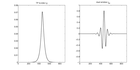
Figure 4: Discrete TP function and its dual $\gamma_{20}$ for $a=20$ and $M=30$.

Sometimes the frame bounds in the discrete case may be better than in the continuous case. Therefore the discrete TP functions or EB-splines may even provide Riesz bases at the critical density, as is explained in the following recent result.

Proposition 18.

[24],[36] Let $g$ be a continuous TP function as in (9), including the infinite type with $\eta=0$. Assume $\alpha=M\in\mathbb{N}$ and let $\beta=1/M$ and $K\in\mathbb{N}$ such that $K/M\in\mathbb{N}$. If $K/M$ is odd, then $\mathcal{G}(P_{K}Sg,\alpha,\beta)$ is a basis of $\mathbb{C}^{K}$.

In addition, assume that $g$ is even, which means that $\{\delta_{\nu}\mid\delta_{\nu}>0\}=\{-\delta_{\nu}\mid\delta_{\nu}<0\}$. If $M$ is odd, then $\mathcal{G}(P_{K}Sg,\alpha,\beta)$ is a basis of $\mathbb{C}^{K}$.

Remark 19.

In the critical case $\alpha\beta=1$ the computation of the dual window $\gamma$ cannot be performed by the aforementioned discretization procedure, as the Gabor system $\mathcal{G}(g,\alpha,\beta)$ is not a frame in $L^{2}(\mathbb{R})$. In this case, the usual method using the discrete Fourier transform and the discrete Zak transform of $P_{K}S\tilde{g}$ should be applied for the computation of the discrete dual window [37].

Appendix

In the appendix we provide the technical details of the proofs of the main theorems. The proof of Theorem 8 depends heavily on [15, Theorem 9].

Proof:

The pre-Gramian is bounded on $\ell^{2}(\mathbb{Z})$ as a consequence of the exponential decay of $g$ and Schur’s test. Therefore the finite sections $P_{L}(x)=\mathcal{P}_{{\boldsymbol{r}}({\boldsymbol{n}})}\,P_{g}(x)\,\mathcal{P}_{\boldsymbol{n}}$ are uniformly bounded.

To prove the existence of a lower bound $A$, we construct a left inverse of $P_{L}(x)$ by adapting the proof of [15, Theorem 9]. By step 2 of Algorithm 5 $P_{L}(x)$ has columns indexed by $k,k_{1}-L\leq k\leq k_{2}+L$ and rows indexed by $j,i_{1}(L)\leq j\leq i_{2}(L)$, thus every left-inverse $Q_{L}(x)$ has columns indexed by $i_{1}(L)\leq j\leq i_{2}(L)$ and rows indexed by $k_{1}-L\leq k\leq k_{2}+L$. We will construct these rows one by one in three steps.

Step 1. For every index $-L\leq\ell\leq L$, we choose the following submatrix $R_{\ell}$ of $P_{L}(x)$. Given $x$ and $\ell\in\mathbb{Z}$, we choose $y_{\ell}\in[0,\alpha)$ and $j_{\ell}\in\mathbb{Z}$, such that

$$y_{\ell}=x+j_{\ell}\alpha-\frac{\ell}{\beta}.$$

Then we define the matrix $R_{\ell}=P_{0}(y_{\ell})$ by using the same definitions as in step 3 of Algorithm 5 with $L=0$; i.e., we let

$$i_{1}^{\ell}(0) =\left\lfloor\frac{k_{1}+m-1}{\alpha\beta}-\frac{y_{\ell}}{\alpha}\right\rfloor+1,$$

$$i_{2}^{\ell}(0) =\left\lceil\frac{k_{2}-n+1}{\alpha\beta}-\frac{y_{\ell}}{\alpha}\right\rceil-1,$$

and

$$R_{\ell}=\left(r_{\ell;j,k}\right)_{i_{1}^{\ell}(0)\leq j\leq i_{2}^{\ell}(0),~{}k_{1}\leq k\leq k_{2}},$$

with $r_{\ell;j,k}=g\left(y_{\ell}+j\alpha-\frac{k}{\beta}\right)$. Note that

$$y_{\ell}+j\alpha-\frac{k}{\beta}=x+(j+j_{\ell})\alpha-\frac{\ell+k}{\beta}.$$

Hence, the columns of $R_{\ell}$, as indexed by $k_{1}\leq k\leq k_{2}$, correspond to sections of columns of $P_{L}(x)$ indexed by $\ell+k_{1}\leq k\leq\ell+k_{2}$. More precisely, $R_{-L}$ contains sections of the first $k_{2}-k_{1}+1$ columns of $P_{L}(x)$; with increasing $\ell$ the selection of columns is shifted to the right; and $R_{L}$ contains sections of the last $k_{2}-k_{1}+1$ columns of $P_{L}(x)$. For the rows of $R_{\ell}$, we observe that

$$i_{1}(L)\leq\left\lfloor\frac{k_{1}+m-1}{\alpha\beta}-\frac{x}{\alpha}+\frac{\ell}{\alpha\beta}\right\rfloor+1=i_{1}^{\ell}(0)+j_{\ell}$$

and $i_{2}(L)\geq i_{2}^{\ell}(0)+j_{\ell}$. To summarize, each $R_{\ell}$ is a $(i_{2}^{\ell}(0)-i_{1}^{\ell}(0)+1)\times(k_{2}-k_{1}+1)$-submatrix of $P_{L}(x)$ with a dimension independent of $|\ell|\leq L$.

Step 2. The arguments in [15, Theorem 8] relate left-inverses of $R_{\ell}=P_{0}(y_{\ell})$ to left-inverses of the biinfinite matrix $P_{g}(y_{\ell})$. It is shown that

• $R_{\ell}$ has full column rank,

• there exists a uniform bound $C>0$, which does not depend on $y_{\ell}\in[0,\alpha)$, and left-inverses $\Gamma_{\ell}$ of $R_{\ell}$ such that

  $$\|\Gamma_{\ell}\|\leq C\quad\mbox{for all}\quad-L\leq\ell\leq L,$$

• the rows with index $k_{1}\leq k\leq 0$ of $\Gamma_{\ell}$ are orthogonal to all columns with index $k^{\prime}>k_{2}-n$ of the biinfinite matrix $P_{g}(y_{\ell})$, and hence orthogonal to all columns $k^{\prime}>\ell+k_{2}-n$ of $P_{L}(x)$. Likewise, rows $0\leq k\leq k_{2}$ of $\Gamma_{\ell}$ are orthogonal to all columns with index $k^{\prime}<\ell+k_{1}+m$ of $P_{L}(x)$.

Step 3. With these properties, we obtain the left-inverse $Q_{L}(x)$ of $P_{L}(x)$ by defining the rows of $Q_{L}(x)$ as follows:

• We start with $\Gamma_{-L}$ and take its rows $k_{1}\leq k\leq 0$ as the first rows of $Q_{L}(x)$, extended by zeros such that

  $$(Q_{L}(x))_{k-L,j+j_{-L}}=\begin{cases}(\Gamma_{-L})_{k,j},&~{}i_{1}^{-L}(0)\leq j\leq i_{2}^{-L}(0),\\ 0,&~{}\mbox{otherwise}.\end{cases}$$

• For $-L+1\leq\ell\leq L-1$ we take the row with index $0$ of $\Gamma_{\ell}$ and extend this row by zeroes,

  $$(Q_{L}(x))_{\ell,j+j_{\ell}}=\begin{cases}(\Gamma_{\ell})_{0,j},&~{}i_{1}^{\ell}(0)\leq j\leq i_{2}^{\ell}(0),\\ 0,&~{}\mbox{otherwise}.\end{cases}$$

• We end with $\Gamma_{L}$ and take its rows $0\leq k\leq k_{2}$ as the last rows of $Q_{L}(x)$, extended by zeros such that

  $$(Q_{L}(x))_{k+L,j+j_{L}}=\begin{cases}(\Gamma_{L})_{k,j},&~{}i_{1}^{L}(0)\leq j\leq i_{2}^{L}(0),\\ 0,&~{}\mbox{otherwise}.\end{cases}$$

It is clear that all entries of $Q_{L}(x)$ are bounded by the constant $C$ in step 2. Moreover, every row and column of $Q_{L}(x)$ has at most

$$\max_{-L\leq\ell\leq L}(i_{2}^{\ell}(0)-i_{1}^{\ell}(0)+1)\leq\frac{k_{2}-k_{1}+1}{\alpha\beta}$$

nonzero entries. Therefore, by Schur’s test, we obtain that

$$\|Q_{L}(x)\|\leq C\,\frac{k_{2}-k_{1}+1}{\alpha\beta}.$$

Since $Q_{L}$ is a left inverse of $P_{L}$, we obtain

$$\lVert c\rVert_{2}=\lVert Q_{L}(x)P_{L}(x)c\rVert_{2}\leq C\,\frac{k_{2}-k_{1}+1}{\alpha\beta}\lVert P_{L}(x)c\rVert_{2},$$

and we may choose $A=(C\,\frac{k_{2}-k_{1}+1}{\alpha\beta})^{-1}$ as a lower bound in (16). This completes the proof of (16). We conclude that $\left\|e_{0}^{T}\,P_{L}(x)^{\dagger}\right\|_{2}\leq C\,\frac{k_{2}-k_{1}+1}{\alpha\beta}=A^{-1}$. Therefore

$$\left\|\gamma_{L}\right\|_{2}^{2} =\int_{-\infty}^{\infty}|\gamma_{L}(x)|^{2}\,dx$$

$$=\beta^{2}\,\int_{0}^{\alpha}\sum_{j\in\mathbb{Z}}|\gamma_{L}(x+j\alpha)|^{2}\,dx$$

$$=\beta^{2}\int_{0}^{\alpha}\left\|e_{0}^{T}\,P_{L}(x)^{\dagger}\right\|_{2}^{2}\,dx\leq\alpha\,\beta^{2}\,A^{-2}.$$

∎

In the following we will need a well known result of Jaffard [38] and Baskakov [39].

Proposition 20.

Let $A=(A_{jk})_{j,k\in\mathbb{Z}}$ be a biinfinite matrix with exponential off-diagonal decay, i.e., there exist constants $C,a>0$, such that

$$|A_{jk}|\leq Ce^{-a|j-k|}\quad\forall j,k\in\mathbb{Z}\,.$$ (23)

If $A$ is invertible, then $A^{-1}$ also possesses exponential off-diagonal decay and there exist $C^{\prime}>0$ and $0<\tilde{a}<a$, such that

$$|(A^{-1})_{jk}|\leq C^{\prime}e^{-\tilde{a}|j-k|}\qquad\forall j,k\in\mathbb{Z}\,.$$

Corollary 21.

Let $A$ be positive and invertible on $\ell^{2}(\mathbb{Z})$ with exponential off-diagonal decay (23) and let $\mathcal{P}_{{\boldsymbol{n}}}A\mathcal{P}_{{\boldsymbol{n}}}$ be a sequence of finite sections. Then every matrix $\mathcal{P}_{{\boldsymbol{n}}}A\mathcal{P}_{{\boldsymbol{n}}}$ is invertible on $\mathcal{P}_{{\boldsymbol{n}}}\ell^{2}(\mathbb{Z})$ and there exist $C^{\prime}>0$ and $\tilde{a},0<\tilde{a}<a$, such that

$$|(\mathcal{P}_{{\boldsymbol{n}}}A\mathcal{P}_{{\boldsymbol{n}}})^{-1}_{jk}|\leq C^{\prime}e^{-\tilde{a}|j-k|}\qquad\text{ for }-n_{1}\leq j,k\leq n_{2}\,.$$ (24)

Proof:

The proof follows [40] and [27]. Let $\mathcal{A}$ be the matrix obtained by stacking the finite sections $\mathcal{P}_{{\boldsymbol{n}}}A\mathcal{P}_{{\boldsymbol{n}}}$ along the diagonal. Then $\mathcal{A}$ possesses exponential off-diagonal decay (23). Since $A$ is invertible and positive, its spectrum $\sigma(A)$ is contained in an interval $[A,B]$ for some $A,B>0$, consequently the spectrum of the restriction of $\mathcal{P}_{\boldsymbol{n}}\,A\,\mathcal{P}_{\boldsymbol{n}}$ on $\mathcal{P}_{\boldsymbol{n}}\ell^{2}(\mathbb{Z})$ is also contained in $[A,B]$ and every finite section is invertible on $\mathcal{P}_{\boldsymbol{n}}\ell^{2}(\mathbb{Z})$. Therefore the stacked matrix $\mathcal{A}$ is invertible on $\oplus\mathcal{P}_{\boldsymbol{n}}\ell^{2}(\mathbb{Z})\simeq\ell^{2}(\mathbb{Z})$. By Proposition 20 $\mathcal{A}^{-1}$ possesses exponential off-diagonal decay. Since $\mathcal{A}^{-1}$ consists of the blocks $(\mathcal{P}_{{\boldsymbol{n}}}A\mathcal{P}_{{\boldsymbol{n}}})^{-1}$, they satisfy $|(\mathcal{P}_{{\boldsymbol{n}}}A\mathcal{P}_{{\boldsymbol{n}}})^{-1}_{jk}|\leq C^{\prime}e^{-\tilde{a}|j-k|}$ for $-n_{1}\leq j,k\leq n_{2}$. ∎

We remark that clearly every finite matrix possesses exponential off-diagonal decay. The point is that the constants may be chosen independently of the size of the finite section.

Proof:

Recall that, for $\boldsymbol{n}=(n_{1},n_{2})\in\mathbb{N}^{2}$, $\mathcal{P}_{\boldsymbol{n}}\,b=(\ldots,0,b_{-n_{1}},b_{-n_{1}+1},\ldots,b_{n_{2}-1},b_{n_{2}},0,\ldots)^{T}$ is the orthogonal projection onto $\mathcal{P}_{\boldsymbol{n}}\,\ell^{2}(\mathbb{Z})\cong\mathbb{C}^{n_{1}+n_{2}+1}$. We write $U_{\boldsymbol{n}}=\mathcal{P}_{\boldsymbol{r}}\,U\,\mathcal{P}_{\boldsymbol{n}}$ for a non-symmetric finite section of $U$. In the assumption of Theorem 9 ${\boldsymbol{r}}$ depends on ${\boldsymbol{n}}$, but we will omit this dependence in the notation. All operator norms are in $\ell^{2}(\mathbb{Z})$.

Let $b:=U\,(U^{*}\,U)^{-1}\,e_{0}$ and $d_{\boldsymbol{n}}:=U_{\boldsymbol{n}}\,(U^{*}_{\boldsymbol{n}}\,U_{\boldsymbol{n}})^{-1}\,e_{0}$. We decompose the norm into three parts

$$\left\|b-d_{\boldsymbol{n}}\right\|_{2} \leq\left\|(U-U\,\mathcal{P}_{\boldsymbol{n}})\,(U^{*}\,U)^{-1}\,e_{0}\right\|_{2}$$

$$+ \left\|U\,\mathcal{P}_{\boldsymbol{n}}\,\Big{(}(U^{*}\,U)^{-1}-(\mathcal{P}_{\boldsymbol{n}}\,U^{*}\,U\,\mathcal{P}_{\boldsymbol{n}})^{-1}\Big{)}\,e_{0}\right\|_{2}$$ (25)

$$+ \left\|U\,\mathcal{P}_{\boldsymbol{n}}\,((\mathcal{P}_{\boldsymbol{n}}\,U^{*}\,U\,\mathcal{P}_{\boldsymbol{n}})^{-1}-U_{\boldsymbol{n}}\,(U^{*}_{\boldsymbol{n}}\,U_{\boldsymbol{n}})^{-1})\,e_{0}\right\|_{2}.$$

1. Note that $U^{*}\,U$ is invertible and positive. Since $U$ fulfills the decay property (18), it is easy to see that the symmetric matrix $U^{*}\,U$ decays exponentially off the diagonal, i.e., for some constants $C,a>0$

$$|(U^{*}U)_{jk}|\leq Ce^{-a|j-k|}\qquad j,k\in\mathbb{Z}\,.$$

By Proposition 20 the inverse matrix inherits the exponential decay, and thus there exist constants $C^{\prime}>0$ and $\tilde{a},0<\tilde{a}<a$, such that $|(U^{*}\,U)^{-1}_{jk}|\leq C^{\prime}e^{-\tilde{a}|j-k|}$ for all $j,k\in\mathbb{Z}$. Hence the entries of the vector $v:=(U^{*}\,U)^{-1}\,e_{0}$ also decay exponentially as

$$\lvert v_{j}\rvert\leq c_{1}\,e^{-\tilde{a}\,\lvert j\rvert}\quad j\in\mathbb{Z}\,.$$ (26)

Since

$$\left\|(I-\mathcal{P}_{\boldsymbol{n}})v\right\|_{2}^{2} =\sum_{j=-\infty}^{-n_{1}-1}|v_{j}|^{2}+\sum_{j=n_{2}+1}^{\infty}|v_{j}|^{2}\leq C^{\prime}\sum_{|j|>n_{0}}e^{-2\tilde{a}|j|}=\mathcal{O}(e^{-2\tilde{a}|j|})\,,$$

the decay property (26) implies that

$$\left\|(U-U\,\mathcal{P}_{\boldsymbol{n}})\,(U^{*}\,U)^{-1}\,e_{0}\right\|_{2} \leq\lVert U\rVert\,\left\|(I-\mathcal{P}_{\boldsymbol{n}})\,v\right\|_{2}\leq c_{2}\,e^{-\tilde{a}\,n_{0}}.$$

2. Since $U^{*}\,U$ is invertible and positive with spectrum $\sigma(U^{*}U)\subseteq[A,B]$ for $A,B>0$, the spectrum of the finite sections $\mathcal{P}_{\boldsymbol{n}}\,U^{*}\,U\,\mathcal{P}_{\boldsymbol{n}}$ on ${\mathcal{P}_{\boldsymbol{n}}\ell^{2}(\mathbb{Z})}$ is also contained in $[A,B]$. As in the finite section method in [40] and with $v=(U^{*}\,U)^{-1}\,e_{0}$, we obtain

$$\left\|((U^{*}\,U)^{-1}-(\mathcal{P}_{\boldsymbol{n}}\,U^{*}\,U\,\mathcal{P}_{\boldsymbol{n}})^{-1})\,e_{0}\right\|_{2}=\left\|(\mathcal{P}_{\boldsymbol{n}}\,U^{*}\,U\,\mathcal{P}_{\boldsymbol{n}})^{-1}\,\mathcal{P}_{\boldsymbol{n}}\,U^{*}\,U\,(\mathcal{P}_{\boldsymbol{n}}-I)\,v\right\|_{2}\leq\lVert(U^{*}\,U)^{-1}\rVert\,\lVert U^{*}\,U\rVert\,\left\|(\mathcal{P}_{\boldsymbol{n}}-I)\,v\right\|_{2}$$

and consequently

$$\left\|U\,\mathcal{P}_{\boldsymbol{n}}\,\big{(}(U^{*}\,U)^{-1}-(\mathcal{P}_{\boldsymbol{n}}\,U^{*}\,U\,\mathcal{P}_{\boldsymbol{n}})^{-1}\big{)}\,e_{0}\right\|_{2} \leq c_{3}\,e^{-\tilde{a}\,n_{0}}$$ .

3. To treat the third term in (25), we need a geometric interpretation of the rows of the Moore-Penrose pseudoinverse. Let

$$b_{\boldsymbol{n}}:=(U\,\mathcal{P}_{\boldsymbol{n}})\,(\mathcal{P}_{\boldsymbol{n}}\,U^{*}\,U\,\mathcal{P}_{\boldsymbol{n}})^{-1}\,e_{0}$$

and $d_{\boldsymbol{n}}$ as above. Then $b_{\boldsymbol{n}}$ is the transpose of the zeroth row of the Moore-Penrose pseudoinverse of $U\,\mathcal{P}_{\boldsymbol{n}}$. By Corollary 21 $(\mathcal{P}_{\boldsymbol{n}}\,U^{*}\,U\,\mathcal{P}_{\boldsymbol{n}})^{-1}$ satisfies (24) independently of ${\boldsymbol{n}}$. Therefore the same argument as in the first part implies the decay property

$$\lvert(b_{\boldsymbol{n}})_{j}\rvert\leq c_{4}\,e^{-\tilde{a}\,\lvert j\rvert}.$$ (27)

It is essential that the constants are independent of ${\boldsymbol{n}}$. Since the Moore-Penrose pseudoinverse of $U\,\mathcal{P}_{\boldsymbol{n}}$ is also a left-inverse, we have

$$b_{\boldsymbol{n}}\,\bot\,V_{\boldsymbol{n}}:=\mathrm{span}\{u_{k}\mid-n_{1}\leq k\leq n_{2},\ k\neq 0\},$$

where $u_{k}$, $k\in\mathbb{Z}$, are the columns of the matrix $U$. Likewise for $U_{\boldsymbol{n}}=\mathcal{P}_{{\boldsymbol{r}}}U\mathcal{P}_{\boldsymbol{n}}$ we have

$$d_{\boldsymbol{n}}\,\bot\,\mathcal{P}_{\boldsymbol{r}}V_{\boldsymbol{n}}\,.$$

Using this orthogonality, we rewrite the vectors $b_{\boldsymbol{n}}$ and $d_{\boldsymbol{n}}$ as follows. Let $\Pi_{W}$ denote the orthogonal projection onto some subspace $W$. Now set

$$\tilde{b}_{\boldsymbol{n}}:=(I-\Pi_{V_{\boldsymbol{n}}})\,u_{0}\quad\text{ and }\quad\tilde{d}_{\boldsymbol{n}}:=(I-\Pi_{\mathcal{P}_{\boldsymbol{r}}V_{\boldsymbol{n}}})\,\mathcal{P}_{\boldsymbol{r}}\,u_{0}\,.$$

Since $b_{\boldsymbol{n}}\in\mathrm{Im}(U\mathcal{P}_{\boldsymbol{n}})$ and $d_{\boldsymbol{n}}\in\mathrm{Im}(U_{\boldsymbol{n}})$, we obtain

$$b_{\boldsymbol{n}}=\frac{\tilde{b}_{\boldsymbol{n}}}{\lVert\tilde{b}_{\boldsymbol{n}}\rVert_{2}^{2}}\quad\text{ and }\quad d_{\boldsymbol{n}}=\frac{\tilde{d}_{\boldsymbol{n}}}{\lVert\tilde{d}_{\boldsymbol{n}}\rVert_{2}^{2}}\,.$$ (28)

The normalization in (28) is obtained from

$$\langle b_{\boldsymbol{n}},u_{0}\rangle=1\quad\text{and}\quad\langle\tilde{b}_{\boldsymbol{n}},u_{0}\rangle=\langle\tilde{b}_{\boldsymbol{n}},\tilde{b}_{\boldsymbol{n}}+\Pi_{V_{\boldsymbol{n}}}\,u_{0}\rangle=\lVert\tilde{b}_{\boldsymbol{n}}\rVert_{2}^{2},$$

$$\langle d_{\boldsymbol{n}},\mathcal{P}_{\boldsymbol{r}}u_{0}\rangle=1\quad\text{and}\quad\langle\tilde{d}_{\boldsymbol{n}},\mathcal{P}_{\boldsymbol{r}}u_{0}\rangle=\langle\tilde{d}_{\boldsymbol{n}},\tilde{d}_{\boldsymbol{n}}+\Pi_{\mathcal{P}_{\boldsymbol{r}}V_{\boldsymbol{n}}}\,\mathcal{P}_{\boldsymbol{r}}u_{0}\rangle=\lVert\tilde{d}_{\boldsymbol{n}}\rVert_{2}^{2}.$$

As the third term in (25) equals $\lVert b_{\boldsymbol{n}}-d_{\boldsymbol{n}}\rVert_{2}$, we first consider $\lVert\tilde{b}_{\boldsymbol{n}}-\tilde{d}_{\boldsymbol{n}}\rVert_{2}$. For this purpose we write

$$\tilde{b}_{\boldsymbol{n}}-\tilde{d}_{\boldsymbol{n}} =(I-\mathcal{P}_{\boldsymbol{r}})\,(u_{0}-\Pi_{V_{\boldsymbol{n}}}\,u_{0})+\Pi_{\mathcal{P}_{\boldsymbol{r}}V_{\boldsymbol{n}}}\,\mathcal{P}_{\boldsymbol{r}}\,u_{0}-\mathcal{P}_{\boldsymbol{r}}\,\Pi_{V_{\boldsymbol{n}}}\,u_{0}$$

$$=(I-\mathcal{P}_{\boldsymbol{r}})\,\tilde{b}_{\boldsymbol{n}}+\Pi_{\mathcal{P}_{\boldsymbol{r}}V_{\boldsymbol{n}}}\,\mathcal{P}_{\boldsymbol{r}}\,(u_{0}-\Pi_{V_{\boldsymbol{n}}}\,u_{0})$$

$$=(I-\mathcal{P}_{\boldsymbol{r}})\,\tilde{b}_{\boldsymbol{n}}+\Pi_{\mathcal{P}_{\boldsymbol{r}}V_{\boldsymbol{n}}}\,\mathcal{P}_{\boldsymbol{r}}\,\tilde{b}_{\boldsymbol{n}}.$$ (29)

By the assumption (19), the truncated columns $\mathcal{P}_{\boldsymbol{r}}\,u_{k}$, with $-n_{1}\leq k\leq n_{2}$ and $k\neq 0$, form a Riesz basis for $\mathcal{P}_{\boldsymbol{r}}V_{\boldsymbol{n}}$ with lower Riesz bound $A$. Furthermore it holds that

$$\left\|\Pi_{\mathcal{P}_{\boldsymbol{r}}V_{\boldsymbol{n}}}\,\mathcal{P}_{\boldsymbol{r}}\,\tilde{b}_{\boldsymbol{n}}\right\|_{2}^{2} \leq A^{-2}\,\sum_{-n_{1}\leq k\leq n_{2},\,k\neq 0}\lvert\langle\Pi_{\mathcal{P}_{\boldsymbol{r}}V_{\boldsymbol{n}}}\,\mathcal{P}_{\boldsymbol{r}}\,\tilde{b}_{\boldsymbol{n}},\mathcal{P}_{\boldsymbol{r}}\,u_{k}\rangle\rvert^{2}$$

$$=A^{-2}\,\sum_{-n_{1}\leq k\leq n_{2},\,k\neq 0}\lvert\langle\mathcal{P}_{\boldsymbol{r}}\,\tilde{b}_{\boldsymbol{n}},u_{k}\rangle\rvert^{2}$$

$$=A^{-2}\,\sum_{-n_{1}\leq k\leq n_{2},\,k\neq 0}\lvert\langle(\mathcal{P}_{\boldsymbol{r}}-I)\,\tilde{b}_{\boldsymbol{n}},u_{k}\rangle\rvert^{2}$$

$$\leq A^{-2}B\,\left\|(\mathcal{P}_{\boldsymbol{r}}-I)\,\tilde{b}_{\boldsymbol{n}}\right\|_{2}^{2},$$

where $B=\lVert U\rVert^{2}$ denotes the Bessel bound of all columns $u_{k}$, $k\in\mathbb{Z}$. Taking the $\ell^{2}$-norm in (Proof:) and substituting the above estimate, we obtain

$$\lVert\tilde{b}_{\boldsymbol{n}}-\tilde{d}_{\boldsymbol{n}}\rVert_{2}\leq c_{5}\,\lVert(I-\mathcal{P}_{\boldsymbol{r}})\,\tilde{b}_{\boldsymbol{n}}\rVert_{2}.$$

We now return to $\lVert b_{\boldsymbol{n}}-d_{\boldsymbol{n}}\rVert_{2}$. It is an easy exercise that for nonzero vectors $y,w$ we have

$$\left\|\frac{y}{\left\|y\right\|_{2}^{2}}-\frac{w}{\left\|w\right\|_{2}^{2}}\right\|_{2}\leq\frac{3\,\left\|y-w\right\|_{2}}{\min\{\left\|y\right\|_{2}^{2},\left\|w\right\|_{2}^{2}\}}.$$

Using once more that $b_{\boldsymbol{n}}\in\mathrm{Im}(U\mathcal{P}_{\boldsymbol{n}})$ and $d_{\boldsymbol{n}}\in\mathrm{Im}(U_{\boldsymbol{n}})$, the assumption (19) implies that

$$0<A\leq\lVert\tilde{b}_{\boldsymbol{n}}\rVert_{2},\lVert\tilde{d}_{\boldsymbol{n}}\rVert_{2}\leq\left\|u_{0}\right\|_{2}\,.$$

By the decay property (27) we obtain

$$\lVert b_{\boldsymbol{n}}-d_{\boldsymbol{n}}\rVert_{2}\leq\tfrac{3}{A^{2}}\,\lVert\tilde{b}_{\boldsymbol{n}}-\tilde{d}_{\boldsymbol{n}}\rVert_{2} \leq\tfrac{3\,c_{5}}{A^{2}}\,\lVert(I-\mathcal{P}_{\boldsymbol{r}})\,\tilde{b}_{\boldsymbol{n}}\rVert_{2}\leq c_{6}\,e^{-\tilde{a}\,n_{0}}.$$

To finish the proof of Theorem 9, we add the three contributions in (25) and obtain the convergence rate (20) with a constant $\tilde{c}=c_{2}+c_{3}+c_{6}$. ∎

References

- [1] M. Dörfler, “Time-frequency analysis for music signals: A mathematical approach,” J. New Music Res., vol. 30, pp. 3–-12, 2001.
- [2] P. C. Russel, J. Cosgrave, D. Tomtsis, A. Vourdas, L. Stergioulas, and G. R. Jones, “Extraction of information from acoustic vibration signals using Gabor transform type devices,” Meas. Sci. Technol., vol. 9, pp. 1282-–1290, 1998.
- [3] F. Hlawatsch and G. Matz, Wireless Communications over Rapidly Time-Varying Cannels. Academic Press, 2011.
- [4] S. Sriram, N. Vijayakumar, P. A. Kumar, A. S. Shetty, V. P. Prasshant, and A. Narayanankutty, “Spectrally efficient multi-carrier modulation using Gabor transform,” Wireless Engineering and Technology, vol. 4, pp. 112–116, 2013.
- [5] S. Blanco, C. E. D’Attellisand S. I. Isaacson, O. Rosso, and R. O. Sirne, “Time-frequency analysis of electroencephalogram series, II: Gabor and wavelet transforms,” Physical Rev. E., vol. 54, pp. 6661–6672, 1996.
- [6] L. Chen, E. Zhao, D. Wang, Z. Han, S. Zhang, and C. Xu, “Feature extraction of EEG signals from epilepsy patients based on Gabor transform and EMD decomposition,” in Sixth International Conference on Natural Computation, 2010.
- [7] O. Christensen, An Introduction to Frames and Riesz Bases. Birkhäuser, 2003.
- [8] K. Gröchenig, Foundations of Time-Frequency Analysis. Birkhäuser, 2001.
- [9] A. J. E. M. Janssen and P. L. Søndergaard, “Iterative algorithms to approximate canonical Gabor windows: computational aspects,” J. Fourier Anal. Appl., vol. 13, pp. 211–241, 2007.
- [10] T. Strohmer, “Numerical algorithms for discrete Gabor expansions,” in Gabor Analysis and Algorithms, H. G. Feichtinger and T. Strohmer, Eds. Birkhäuser, 1998, pp. 267–294.
- [11] Z. Průša, P. L. Søndergaard, N. Holighaus, C. Wiesmeyr, and P. Balazs, “The large time-frequency analysis toolbox 2.0,” in Sound, Music, and Motion, ser. Lecture Notes in Computer Science, M. Aramaki, O. Derrien, R. Kronland Martinet, and S. Ystad, Eds. Springer International Publishing, 2014, pp. 419–442.
- [12] G. Schulz, “Iterative Berechnung der reziproken Matrix,” Z. Angew. Math. Mech., vol. 13, pp. 57–59, 1933.
- [13] A. J. E. M. Janssen, “Analysis of some fast algorithms to compute canonical windows for Gabor frames,” 2002, unpublished.
- [14] ——, “Some iterative algorithms to compute canonical windows for Gabor frames,” Proceedings of IMS Workshop on Time-Frequenzy Analysis and Applications, 2004.
- [15] K. Gröchenig and J. Stöckler, “Gabor frames of totally positive functions,” Duke Math. J., vol. 162, pp. 1003–1031, 2013.
- [16] T. Kloos and J. Stöckler, “Zak transforms and Gabor frames of totally positive functions and exponential B-splines,” J. Approx. Theory, vol. 184, pp. 209–237, 2014.
- [17] K. Gröchenig, “Acceleration of the frame algorithm,” IEEE Trans. Sign. Proc., vol. 41, pp. 3331–3340, 1993.
- [18] H. Hotelling, “Some new methods in matrix calculation,” Ann. Math. Statist., vol. 14, pp. 1–34, 1943.
- [19] S. Karlin, Total Positivity. Stanford University Press Inc., 1968.
- [20] L. L. Schumaker, Spline Functions: Basic Theory. John Wiley and Sons, 1981.
- [21] R. A. DeVore and G. G. Lorentz, Constructive Approximation. Springer, 1993.
- [22] I. J. Schoenberg, “On totally positive functions, Laplace integrals and entire functions of the Laguerre-Pólya-Schur type,” Proc. Natl. Acad. Sci. USA, vol. 33, pp. 11–17, 1947.
- [23] ——, “On Pólya frequency functions. I. The totally positive functions and their Laplace transforms,” J. Anal. Math., vol. 1, pp. 331–374, 1951.
- [24] S. Bannert, K. Gröchenig, and J. Stöckler, “Discretized Gabor frames of totally positive functions,” IEEE Trans. Inform. Theory, vol. 60, pp. 159–169, 2014.
- [25] T. Kloos, “Gabor Frames total-positiver Funktionen endlicher Ordnung,” Diploma thesis, TU Dortmund, 2012.
- [26] A. J. E. M. Janssen, “Duality and biorthogonality for Weyl-Heisenberg frames,” J. Fourier Anal. Appl., vol. 1, pp. 403–436, 1995.
- [27] K. Gröchenig, Z. Rzeszotnik, and T. Strohmer, “Convergence analysis of the finite section method and Banach algebras of matrices,” Integr. Equ. Oper. Theory, vol. 67, pp. 183–202, 2010.
- [28] A. Aldroubi, A. G. Baskakov, and I. A. Krishtal, “Slanted matrices, Banach frames, and sampling,” J. Funct. Anal., vol. 255, pp. 1667–1691, 2008.
- [29] E. Cordero, K. Gröchenig, F. Nicola, and L. Rodino, “Wiener algebras of Fourier integral operators,” J. Math. Pures Appl., vol. 99, pp. 219–233, 2013.
- [30] P. L. Søndergaard, “Gabor frames by sampling and periodization,” Adv. Comput. Math., vol. 27, pp. 355–373, 2007.
- [31] A. J. E. M. Janssen, “The Zak transform: a signal transform for sampled time-continuous signals,” Philips J. Res., vol. 43, pp. 23–69, 1988.
- [32] C. deBoor, A Practical Guide to Splines. Springer, 1978.
- [33] O. Christensen and P. Massopust, “Exponential B-splines and the partition of unity property,” Adv. Comput. Math., vol. 37, pp. 301–318, 2012.
- [34] N. Dyn and A. Ron, “Recurrence relations for Tchebycheffian B-splines,” J. Anal. Math., vol. 51, pp. 118–135, 1988.
- [35] A. Ron, “Exponential box splines,” Constr. Approx., vol. 4, pp. 357–378, 1988.
- [36] T. Kloos, “Zeros of the Zak transform of totally positive functions,” J. Fourier Anal. Appl., DOI 10.1007/s00041-015-9402-5.
- [37] H. Bölcskei, F. Hlawatsch, “Discrete Zak transforms, polyphase transforms, and applications,” IEEE Trans. Sign. Proc., vol. 45, pp. 851–866, 1997.
- [38] S. Jaffard, “Propriétés des matrices ”bien localisées” près de leur diagonale et quelques applications,” Ann. Inst. H. Poincaré Anal. Non Linéaire, vol. 7, pp. 461–476, 1990.
- [39] A. G. Baskakov, “Wiener’s theorem and asymptotic estimates for elements of inverse matrices,” Funktsional. Anal. i Prilozhen, vol. 24, pp. 64–65, 1990.
- [40] R. Hagen, S. Roch, and B. Silbermann, -Algebras and Numerical Analysis. Monogr. Textbooks Pure Appl. Math., vol. 236, Verlag C. H. Beck, 2001.