Bill2d – a software package for classical two-dimensional Hamiltonian systems

Abstract

We present Bill2d, a modern and efficient C$++$ package for classical simulations of two-dimensional Hamiltonian systems. Bill2d can be used for various billiard and diffusion problems with one or more charged particles with interactions, different external potentials, an external magnetic field, periodic and open boundaries, etc. The software package can also calculate many key quantities in complex systems such as Poincaré sections, survival probabilities, and diffusion coefficients. While aiming at a large class of applicable systems, the code also strives for ease-of-use, efficiency, and modularity for the implementation of additional features. The package comes along with a user guide, a developer’s manual, and a documentation of the application program interface (API).

PROGRAM SUMMARY
Program Title: Bill2d
Journal Reference:
Catalogue identifier:
Licensing provisions: GNU General Public License version 3
Programming language: C$++$(14)
Computer: Tested on x86 and x86_64 architectures.
Operating system: Tested on Linux, and OS X versions 10.9-10.11.
Compilers: C$++$14 compliant compiler. Tested compilers: Clang 3.7, GCC 4.9-5.2, and Intel C$++$ compiler 15.
RAM: Simulation dependent: kilobytes to gigabytes
Parallelization: Shared memory parallelization when simulating ensembles of systems.
Keywords: Classical mechanics; billiards; nonlinear dynamics; chaos; transport; diffusion; numerical simulations; molecular dynamics
Classification: 4.3 Differential equations, 7.8 Structure and Lattice dynamics, 7.9 Transport properties, 7.10 Collisions in solids, 16.9 Classical methods
External routines/libraries:
Boost, CMake, GSL, HDF5; and optionally GoogleMock, GoogleTest, and Doxygen
Nature of problem:
Numerical propagation of classical two-dimensional single and many-body systems, possibly in a magnetic field, and calculation of relevant quantities such as Poincaré sections, survival probabilities, diffusion coefficients, etc.
Solution method:
Symplectic numerical integration of Hamilton’s equations of motion in Cartesian coordinates, or solution of Newton’s equations of motion if in a magnetic field. The program implements several well-established algorithms.
Restrictions:
Pointlike particles with equal masses and charges, although the latter restrictions are easy to lift.
Unusual features:
Program is efficient, extremely modular and easy to extend, and allows arbitrary particle-particle interactions.
Additional comments:
The source code is also available at https://bitbucket.org/solanpaa/bill2d. See README for locations of user guide, developer manual, and API docs.
Running time:
From milliseconds to days, depends on type of simulation.

1 Introduction

Hamiltonian systems still offer a wide range of yet unexplored territories and interests for the study of nonlinear dynamics and chaos. This is evident from the recent progress, e.g., in the study of transmission, escape rates, and survival probabilities of open systems and recurrences in closed systems  [1, 2, 3, 4, 5, 6, 7, 8, 9, 10], stickiness and marginally unstable periodic orbits [10, 11, 12, 13], and detailed analysis of the graphene-like Lorentz gas and related systems [14, 15, 16, 17, 18, 19, 20, 21], and this list barely scratches the surface. As pointed out by Bunimovich and Vela-Arevalo, “Chaos theory is very much alive” [1].

Two-dimensional (2D) Hamiltonian systems (i.e., with two coordinate dimensions), such as dynamical billiards, have the advantage of being simple, but not too simple. That is, they are easy to study and visualize, but even a single-particle system can display a large variety of complex phenomena of Hamiltonian chaos. Many of these systems can also be realized as semiconductor nanostructures [22, 23]. While governed by quantum mechanics, these nanostructures have ballistic regions where a classical treatment applies to some extent [5].

2D billiards (including soft potentials) with point-like particles can be simulated either using the exact solution, the exact Poincaré map, or by solving Hamilton’s or Newton’s equations of motion. The exact solution is often unknown, apart from single-particle systems with simple geometries. Therefore, one often resorts to numerical solution of the classical equations of motion.

In this paper we introduce Bill2d, a code for generic, classical 2D systems with a focus on the study of chaos and nonlinear dynamics. The code can handle single or many particles, hard-wall boundaries (as in traditional billiards), particle-particle interactions, external potentials, periodic systems, a magnetic field, etc. Written in modern C$++$, Bill2d is modular and easy to extend without sacrificing speed or ease-of-use.

The paper is organized as follows: In Sec. 2 we describe the class of systems to which Bill2d can be applied. In Sec. 3 we briefly discuss the numerical propagation algorithms and in Sec. 4 implementation and structure of the code. In Sec. 5 we give a few numerical examples of what can be simulated with Bill2d. In Sec. Sec. 6 we finish with a brief summary of the paper.

2 Systems

2.1 Overview

Bill2d is designed for classical dynamics of interacting particles in two-dimensions. The program can deal with both traditional billiards with hard-wall boundaries as well as with soft external potentials including also periodic systems. Single- and multiparticle systems with a generic form for the particle-particle interaction can be simulated, and an external magnetic field can be included. Transport calculations are supported by allowing the creation and removal of particles during the simulation.

When treating systems without a magnetic field, we propagate the particles via Hamilton’s equations of motion using symplectic algorithms. Systems with a magnetic field are propagated using Newton’s equations of motion.

The program is written using Cartesian coordinates and atomic units, i.e., we set masses, charges, and the Coulomb constant to unity. All the particles are point-like and with equal masses and charges (as, e.g., electrons in semiconductors), although the equal mass and charge requirement can be lifted with minor modifications to the code.

To clarify, systems without an external magnetic field are described by the $N$-particle Hamiltonian ($N\geq 1$)

$$H=\sum\limits_{i=1}^{N}\left(\frac{1}{2}\|\mathbf{p}_{i}\|^{2}+V(\mathbf{r}_{i})\right)+\sum\limits_{i<j}W(\mathbf{r}_{i},\mathbf{r}_{j}),$$ (1)

where $\mathbf{r}_{i}$ and $\mathbf{p}_{i}$ are the position and momentum of the $i$th particle, $V(\mathbf{r})$ is the total external single-particle potential, and $W(\mathbf{r}_{i},\mathbf{r}_{j})$ the interparticle potential. In principle, potentials $V$ and $W$ can be arbitrary, but in the case of attracting singularities, new propagation algorithms should be implemented.

When the system includes a magnetic field, we use the Newtonian formulation instead of Hamiltonian formulation. The equations of motion are

$$\begin{split}\frac{{\rm d}^{2}\mathbf{r}_{i}}{{\rm d}t^{2}}=&-\nabla_{\mathbf{r}_{i}}V(\mathbf{r}_{i})-\sum\limits_{j\neq i}\nabla_{\mathbf{r}_{i}}W(\mathbf{r}_{i},\mathbf{r}_{j})\\ &+B\left(\frac{{\rm d}r_{i,y}}{{\rm d}t}\mathbf{e}_{x}-\frac{{\rm d}r_{i,x}}{{\rm d}t}\mathbf{e}_{y}\right){},\end{split}$$ (2)

where $r_{i,x/y}$ is the $x$ or $y$  coordinate of the position of the $i$th particle and $\mathbf{e}_{x/y}$ the corresponding unit vector. The first term in Eq. (2) is the force due to the external potential, the second term the interparticle interaction, and the third term the Lorentz force with the magnetic flux density $B$ perpendicular to the two-dimensional plane.

The systems can also include hard-wall billiard boundaries. The (fully elastic) collision of the $i$th particle with the billiard boundary is described by the transformation

$$\mathbf{r}_{i} \to\mathbf{r}_{i}$$ (3)

$$\mathbf{p}_{i} \to\mathbf{p}_{i}-2\left[\mathbf{n}(\mathbf{r}_{i})\cdot\mathbf{p}_{i}\right]\,\mathbf{n}(\mathbf{r}_{i}),$$

where $\mathbf{n}(\mathbf{r}_{i})$ is a unit vector perpendicular to the corresponding boundary at position $\mathbf{r}_{i}$.

2.2 Note on Coulomb interaction and the interaction strength parameter

When describing Coulomb-interacting systems, we introduce the interaction strength parameter $\alpha$. Essentially the Coulomb-potential is given by

$$W(\mathbf{r}_{i},\mathbf{r}_{j})=\sum_{i<j}\frac{\alpha}{\|\mathbf{r}_{i}-\mathbf{r}_{j}\|}.$$ (4)

By fixing the total energy and length scale (i.e., the size of the billiard table) of the system, we can actually study all length and energy scales of all geometrically similar systems just by varying $\alpha$.

Naturally this trick works only if the system does not have external potentials (apart from a hard-wall boundary) or a magnetic field. In case of a magnetic field and/or external potentials, also those have to be adjusted. For detailed derivation of the corresponding scale transformations and demonstration of the idea, we refer the reader to Appendix B of Ref. [3].

3 Algorithms

3.1 Propagation without a magnetic field

The propagator, for Hamiltonian systems with the Hamiltonian $H$, is

$$\exp(t\left\{\cdot,H\right\}),$$ (5)

where $\left\{\cdot,\cdot\right\}$ is the Poisson bracket operator.

The systems we are interested in are described by Hamiltonians [Eq. (1)] that can be split to two parts as $H=K(\mathbf{p})+U(\mathbf{r})$, where all the momentum dependence is in $K$, and all the coordinate dependence is in $U$. As the Hamiltonian is separable, there are plentiful of explicit algorithms for the time propagation. This is in contrast to general Hamiltonian systems where the symplectic integrators are typically implicit and hence computationally more demanding.

The algorithms we have implemented are based on split operator schemes, where the propagator, $\exp\left(\Delta t\left\{\cdot,H\right\}\right)$ is approximated by some product of $\exp\left(const\cdot\Delta t\left\{\cdot,K\right\}\right)$ and $\exp\left(const\cdot\Delta t\left\{\cdot,U\right\}\right)$. The operation of these latter exponentials can be carried out exactly – to numerical accuracy – allowing for an easy implementation of split operator schemes. For example, the velocity Verlet scheme [24] can be expressed as

$$\mathrm{e}^{\Delta t\left\{\cdot,H\right\}}\approx\mathrm{e}^{\frac{1}{2}\Delta t\left\{\cdot,U\right\}}\mathrm{e}^{\Delta t\left\{\cdot,K\right\}}\mathrm{e}^{\frac{1}{2}\Delta t\left\{\cdot,U\right\}}.$$ (6)

We have implemented symplectic algorithms of orders 2–6 for systems without a magnetic field. The algorithms (from Refs. [24, 25, 26, 27]) are specified in USERGUIDE.

3.2 Propagation in a magnetic field

In a magnetic field, the systems are propagated via Newton’s equations of motion [Eq. (2)] as we are unaware of any efficient symplectic algorithms for this class of systems. We have implemented two algorithms: (i) the second order Taylor expansion scheme developed by Spreiter and Walter [28] and (ii) the fourth order algorithm developed by Y. He et al. in Ref. [29].

The algorithm by Spreiter and Walter has been later shown to be an energy conserving split-operator scheme [30], and the fourth order algorithm is volume preserving (and also preserves the total energy extremely well) [29]. These schemes explicitly incorporate the effects of the magnetic field into the propagation formulas, and allow – in principle – an arbitrarily strong magnetic field without the need for a smaller time step.

4 Implementation

4.1 Overview

Bill2d is designed as a modular, object-oriented package, and is written in standards-compliant C$++$ following the International Standard ISO/IEC 14882:2014(E) Programming Language C++ (aka C$++$14) [31]. The package contains three binaries: bill2d for single simulation of a (many-body) trajectory, bill2d_escape for the calculation of escape rates in open billiards, and bill2d_diffusion_coefficient for the calculation of diffusion coefficients in periodic systems. All the binaries obey similar inputs; more details are given in USERGUIDE.

The binaries make use of the libbill2d library, which is created during the compilation process. Most of the classes and methods of the library are enclosed in the namespace bill2d. This library can be used for easy implementation of additional binaries. A tutorial for developing new binaries and features can be found in docs/developer_manual.pdf, which also describes the implementation in detail.

4.2 Input and initial positions

The class Parser handles parsing of the input either from command line, configuration file, or a combination of these. The option parsing is implemented with the help of Boost::program_options library.

The input defines the system (number of particles, magnetic field, potentials, periodicity, etc.) and simulation parameters (algorithm, time step, simulation time, etc.). The initial positions and velocities of the particles can either be supplied manually, or Bill2d can randomize them.

The default random initial conditions are calculated as follows: First the initial positions of the particles are randomized either within a given hard-wall billiard table, a unit cell, or a user-supplied rectangular area. Next, the kinetic energy is distributed evenly among the particles, and the directions of the velocities are randomized. Note also that implementation of new randomization procedures for the initial conditions is easy.

4.3 Application programming interface

The package consists of several classes each designed usually for a single purpose: Table handles collisions with hard-wall boundaries, Datafile handles saving of data, etc. The easiest way for a developer to create instances of all the necessary classes is to use the Parser to get all the input parameters bundled in an instance of ParameterList, which can then be passed on to BilliardFactory. This factory class can be used to create instances of Billiard, which bundles all the other necessary objects together. Furthermore, instances of the Billiard class save data automatically during simulation and upon destruction. In all simplicity, a minimal working example could be as follows.

⬇

#include "bill2d/parser.hpp"

#include "bill2d/billiard_factory.hpp"

using namespace bill2d;

int main( int argc, char *argv[] ) {

Parser@ parser( argc, argv );

auto params =

parser.getParameterList();

BilliardFactory@ factory( params );

auto billiard = factory.get_bill();

// Set initial condition

billiard->prepare(3.0 /* energy */);

// Get reference to time.

// This variable is kept up to date.

const auto& time =

billiard->get_time();

while ( time < 5.0 )

billiard->propagate();

} // Saving data upon

// destruction of billiard

For more complex examples, see files src/bill2d_single_run.cpp, src/bill2d_escape.cpp, and src/bill2d_diffusion_coefficient.cpp, and the developer manual docs/developer_manual.pdf

4.4 Datafile

The program saves its data (trajectories, energies, etc.) to a HDF5-file. The datafile can be accessed afterwards for analysis with several tools including, e.g., the ready made scripts included in the Bill2d package, different programming languages (at least Python, C, C$++$, Fortran, and Java) and programs such as Matlab and Mathematica. The USERGUIDE describes in more detail how to access the HDF5-files.

4.5 Test suite

The software is bundled with comprehensive unit tests, which currently cover most of the program. Additional tests can be run with the Python script test/propagator_tests.py, which requires the user to download reference data from the URL specified in README.

5 Numerical examples

5.1 Trajectories

A fundamental concept in classical point-particle mechanics is a trajectory, i.e., the curve that the particle draws in the coordinate space. In Fig. 1 we show a single-particle trajectory in the Bunimovich mushroom billiards [32] calculated with the bill2d binary. The trajectory has been drawn with the draw_trajectories script, which is bundled with the software package.

Similarly, one can consider trajectories of a many-particle system, as in Fig. 2, which shows 15 Coulomb-interacting particles inside a circular billiard table. Here several different trajectories share the same color.

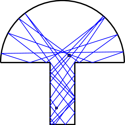
Figure 1: Single-particle billiards in a Bunimovich mushroom.

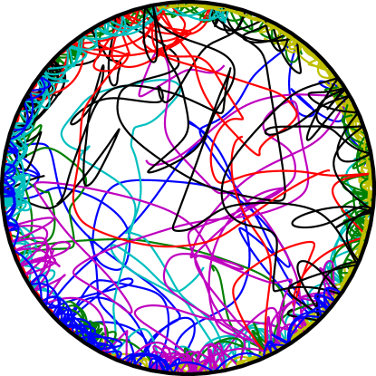
Figure 2: Circular billiards with 15 Coulomb-interacting particles.

5.2 Poincaré sections

The phase space can be studied by selecting a two-dimensional subspace of the full phase space, and visualizing all crossings of a phase space trajectory (or trajectories) with the chosen subspace, which is called the Poincaré section.

In Fig. 3 we show the Poincaré section of a single-particle elliptic billiards in a magnetic field calculated with the bill2d binary; several initial positions are considered in this figure. Here the Poincaré section shows the collisions with the billiard table, parametrized by the arc length $s$ and the tangential velocity $v_{\parallel}$. The Poincaré section consists of several elliptic and parabolic KAM islands (after Kolmogorov, Arnold, and Moser [33, 34, 35]) that correspond to regular motion, as well as a chaotic sea indicated by irregularly distributed points. This system has previously been studied in, e.g., Ref. [36].

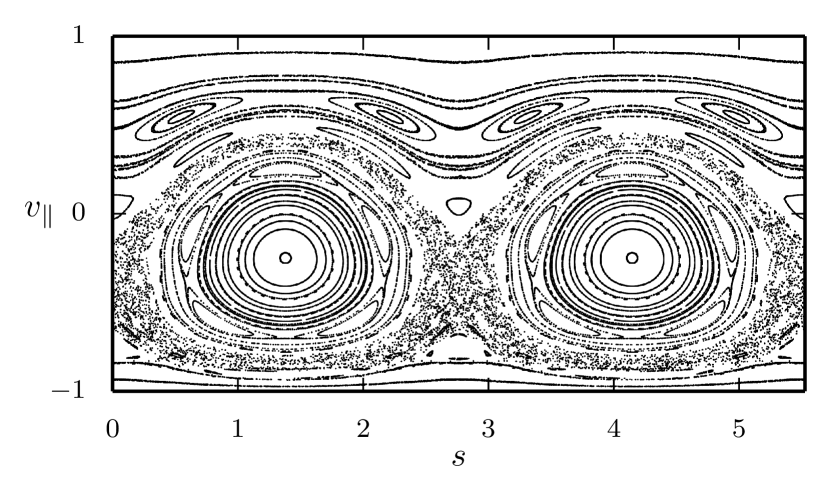
Figure 3: Poincaré section of an elliptic billiard with semi-major and -minor axes 1 and $3/4$ in a magnetic field with Larmor radius $r=3$.

5.3 Escape rates in open billiards

Open billiards have one or many holes in the billiard boundary through which the particle(s) can escape the system. The object of interest here is the survival probability or the escape rate. The survival probability $P_{\mathrm{s}}(t)$ gives the probability that the particle has not exited the system before time $t$, and the escape rate $p_{\mathrm{e}}(t)$ gives the probability density of escape within a narrow time interval around $t$. These two are naturally related by

$$\frac{\mathrm{d}P_{\mathrm{s}}(t)}{\mathrm{d}t}=-p_{\mathrm{e}}(t).$$ (7)

In Fig. 4 we show the escape rate for a single particle square billiards in a magnetic field, as calculated with the bill2d_escape binary (blue line). The square has side length of unity, with a hole of length $0.3$, and the magnetic field is such that the Larmor radius is $0.5075$. As a reference, we have calculated the escape rate using an analytical mapping between boundary collisions (red line), which is available for such a simple system. The results are nearly identical all the way to very small escape rates (i.e., very rare trajectories). Note that trajectories that can never escape the system are not included in the data.

After a brief initial period, the escape-rate curve is found to be a combination of exponential and algebraic functions, which is typical for systems with a mixed phase space in the corresponding closed system [37]. In this system the mixed phase space (studied, e.g., in Ref. [38]) is evident from, e.g., the regular characteristics of the example trajectory in the inset of Fig. 4.

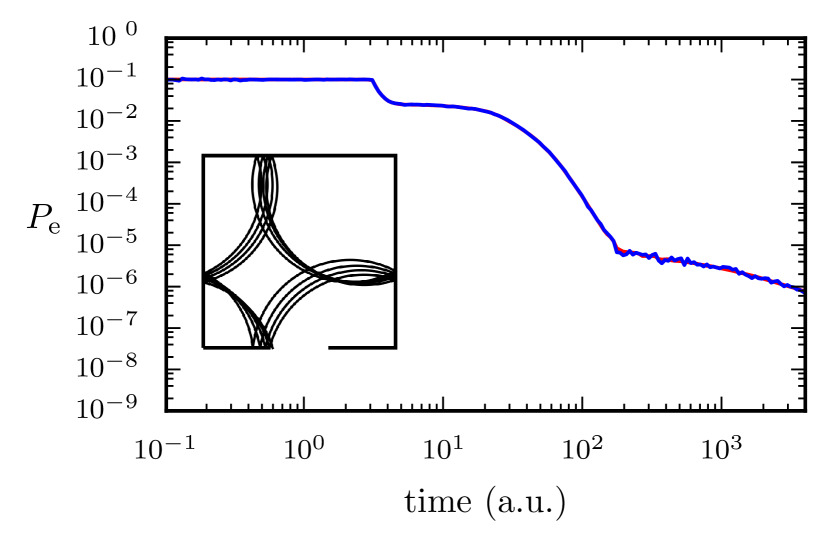
Figure 4: Escape rate for a single-particle in square billiards in a magnetic field with Larmor radius $0.5075$. The result demonstrates a combination of algebraic and exponential behavior as a function of time. The escape rate computed from an ensemble of trajectories using bill2d_escape is shown as a blue line, and a reference curve computed with an analytical collision map is shown as a red line.

5.4 Diffusion in periodic lattices

When studying planar billiards in periodic structures, it is of interest to see how the particle diffuses – on the average – in the system. The diffusion coefficient is defined as

$$D=\lim\limits_{t\to\infty}\frac{\langle\|\mathbf{r}(t)-\mathbf{r}(0)\|^{2}\rangle}{4t},$$ (8)

where $\langle\cdot\rangle$ is the average over all possible initial configurations.

Let us consider a hexagonal antidot lattice of scatterers with lattice constant unity (see the inset of Fig. 5). Each scatterer produces a repulsive potential of the form $V_{\alpha}(\mathbf{r})=\left(1+\exp[(\|\mathbf{r}-\mathbf{R}_{\alpha}\|-d)/\sigma]\right)^{-1}$. This is defined by three parameters: scatterer position $\mathbf{R}_{\alpha}$, radius $d$, and the softness of the potential $\sigma$. The system thus corresponds to a Lorentz gas – an extensively studied system in chaos theory – with soft boundaries [14].

The mean squared displacement (MSD) $\langle\|\mathbf{r}(t)-\mathbf{r}(0)\|^{2}\rangle$ of a particle in the antidot lattice is shown in Fig. 5 as a function of time. In this example the total energy $E=\frac{1}{2}$, scatterer radius $d=0.15$, and scatterer softness $\sigma=0.1$. The MSD has a power law behavior $\text{MSD}\sim t^{\gamma}$ with $\gamma\approx 2$, which means that the system is superdiffusive, and the diffusion coefficient (8) diverges. This behavior is due to large number of trajectories demonstrating Levý walk characteristics or even purely ballistic behaviour.

In this example we have simulated an ensemble of $5500$ trajectories, which results in approx. 2.5 % relative standard error of the mean for the MSD at $t=4000$. The calculation was done with the binary bill2d_diffusion_coefficient.

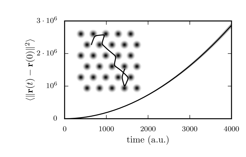
Figure 5: Mean squared displacement for a soft Lorentz gas with scatterer radius $d=0.15$, softness $\sigma=0.1$, energy $E=\frac{1}{2}$ behaves as a power law in time ($\sim t^{\gamma}$) with exponent $\gamma\approx 2$. The inset shows a single trajectory in the system.

6 Summary

The software package Bill2d is a versatile and efficient tool to simulate classical two-dimensional systems. It supports, e.g., single and many-body simulations including varying particle number, interparticle interactions, different external potentials, a magnetic field, periodic boundaries, and hard-wall billiard tables. In addition to the versatility, the main strengths of Bill2d are its modular, object-oriented design, which allows easy implementation of new features, and a clear and extensively documented source code.

Bill2d has already been used in several studies including, e.g., chaotic properties of many-body billiards [3, 2], nonlinear dynamics of Wigner molecules [39], and diffusion in periodic lattices [40]. The package can also be readily applied to, e.g., classical studies of transport properties in two-dimensional structures.

7 Acknowledgments

We are grateful for Stack Overflow user Rob_ϕ for his help with Boost::program_options, Trond Norbye for his blog post on Python scripts and Automake, David Corvoysier for his blog post on GoogleTest and CMake, Ryan Pavlik for his GetGitRevisionDescription CMake-module, Mark Moll for his post on CMake mailing list about CMake and Python, and Visa Nummelin for initial development of the reference code for single-particle magnetic rectangular billiards. We also thank Johannes Nokelainen, Sol Gil Gallegos, and Rainer Klages for useful discussions. Likewise, we thank all our users for bug reports. This work was supported by the Academy of Finland and the Finnish Cultural Foundation. We also acknowledge CSC – the Finnish IT Center for Science for computational resources.

References

- [1] L. A. Bunimovich, L. V. Vela-Arevalo, Some new surprises in chaos, Chaos 25 (2015) 097614. doi:10.1063/1.4916330.
- [2] J. Solanpää, J. Nokelainen, P. J. J. Luukko, E. Räsänen, Coulomb-interacting billiards in circular cavities, J. Phys. A 46 (2013) 235102. doi:10.1088/1751-8113/46/23/235102.
-
[3]
J. Solanpää,
Nonlinear
dynamics and chaos in classical Coulomb-interacting many-body billiards,
Master’s thesis, University of Jyväskylä (2013).
URL http://www.solanpaa.fi/documents/solanpaa_msc_thesis.pdf - [4] C. P. Dettmann, M. R. Rahman, Survival probability for open spherical billiards, Chaos 24 (2014) 043130. doi:10.1063/1.4900776.
- [5] C. P. Dettmann, O. Georgiou, Transmission and reflection in the stadium billiard: Time-dependent asymmetric transport, Phys. Rev. E 83 (2011) 036212. doi:10.1103/PhysRevE.83.036212.
- [6] G. Cristadoro, R. Ketzmerick, Universality of algebraic decays in hamiltonian systems, Phys. Rev. Lett. 100 (2008) 184101. doi:10.1103/PhysRevLett.100.184101.
- [7] C. P. Dettmann, E. D. Leonel, Escape and transport for an open bouncer: Stretched exponential decays, Physica D 241 (2012) 403 – 408. doi:10.1016/j.physd.2011.10.012.
- [8] M. S. Custódio, M. W. Beims, Intrinsic stickiness and chaos in open integrable billiards: Tiny border effects, Phys. Rev. E 83 (2011) 056201. doi:10.1103/PhysRevE.83.056201.
- [9] O. Georgiou, C. P. Dettmann, E. G. Altmann, Faster than expected escape for a class of fully chaotic maps, Chaos 22 (2012) 043115. doi:10.1063/1.4766723.
- [10] C. P. Dettmann, O. Georgiou, Open mushrooms: stickiness revisited, J. Phys. A 44 (2011) 195102. doi:10.1088/1751-8113/44/19/195102.
- [11] S. Tsugawa, Y. Aizawa, Stagnant motion in Hamiltonian dynamics —mushroom billiard case with smooth outermost KAM tori—, J. Phys. Soc. Jpn., 83 (2014) 024002. doi:10.7566/JPSJ.83.024002.
- [12] L. A. Bunimovich, L. V. Vela-Arevalo, Many faces of stickiness in Hamiltonian systems, Chaos 22 (2012) 026103. doi:10.1063/1.3692974.
- [13] L. A. Bunimovich, Fine structure of sticky sets in mushroom billiards, J. Stat. Phys. 154 (2014) 421–431. doi:10.1007/s10955-013-0898-2.
- [14] C. P. Dettmann, Diffusion in the Lorentz gas, Commun. The. Phys. 62 (2014) 521. doi:10.1088/0253-6102/62/4/10.
- [15] T. Harayama, R. Klages, P. Gaspard, Deterministic diffusion in flower-shaped billiards, Phys. Rev. E 66 (2002) 026211. doi:10.1103/PhysRevE.66.026211.
- [16] T. Gilbert, H. C. Nguyen, D. P. Sanders, Diffusive properties of persistent walks on cubic lattices with application to periodic Lorentz gases, Journal of Physics A: Mathematical and Theoretical 44 (2011) 065001. doi:10.1088/1751-8113/44/6/065001.
- [17] G. Cristadoro, T. Gilbert, M. Lenci, D. P. Sanders, Measuring logarithmic corrections to normal diffusion in infinite-horizon billiards, Phys. Rev. E 90 (2014) 022106. doi:10.1103/PhysRevE.90.022106.
- [18] J. Wiersig, K.-H. Ahn, Devil’s staircase in the magnetoresistance of a periodic array of scatterers, Phys. Rev. Lett. 87 (2001) 026803. doi:10.1103/PhysRevLett.87.026803.
- [19] M. Khoury, A. M. Lacasta, J. M. Sancho, A. H. Romero, K. Lindenberg, Charged particle transport in antidot lattices in the presence of magnetic and electric fields: Langevin approach, Phys. Rev. B 78 (2008) 155433. doi:10.1103/PhysRevB.78.155433.
- [20] J. Yang, H. Zhao, Anomalous diffusion among two-dimensional scatterers, Journal of Statistical Mechanics: Theory and Experiment 2010 (2010) L12001. doi:10.1088/1742-5468/2010/12/L12001.
- [21] N.-C. Panoiu, Anomalous diffusion in two-dimensional potentials with hexagonal symmetry, Chaos 10 (2000) 166–179. doi:http://dx.doi.org/10.1063/1.166484.
- [22] K. Nakamura, T. Harayama, Quantum Chaos and Quantum Dots, Oxford University Press, Oxford, 2003.
- [23] A. P. Micolich, A. M. See, B. C. Scannell, C. A. Marlow, T. P. Martin, I. Pilgrim, A. R. Hamilton, H. Linke, R. P. Taylor, Is it the boundaries or disorder that dominates electron transport in semiconductor ‘billiards’?, Fortschr. Physik 61 (2013) 332 – 347. doi:10.1002/prop.201200081.
- [24] M. P. Allen, D. J. Tildesley, Computer Simulation of Liquids, Oxford University Press (USA), 1989. doi:10.1016/0167-7322(88)80022-9.
- [25] R. I. McLachlan, On the numerical integration of ordinary differential equations by symmetric composition methods, SIAM J. Sci. Comput. 16 (1995) 151 – 168. doi:10.1137/0916010.
- [26] M. Suzuki, General nonsymmetric higher-order decomposition of exponential operators and symplectic integrators, J. Phys. Soc. Jpn. 61 (1992) 3015 – 3019. doi:10.1143/JPSJ.61.3015.
- [27] H. Yoshida, Construction of higher order symplectic integrators, Phys. Lett. A 150 (1990) 262 – 268. doi:10.1016/0375-9601(90)90092-3.
- [28] Q. Spreiter, M. Walter, Classical molecular dynamics simulation with the velocity Verlet algorithm at strong external magnetic fields, J. Comp. Phys. 152 (1999) 102 – 119. doi:10.1006/jcph.1999.6237.
- [29] Y. He, Y. Sun, J. Liu, H. Qin, Volume-preserving algorithms for charged particle dynamics, J. Comput. Phys. 281 (2015) 135 – 147. doi:10.1016/j.jcp.2014.10.032.
- [30] S. A. Chin, Symplectic and energy-conserving algorithms for solving magnetic field trajectories, Phys. Rev. E 77 (2008) 066401. doi:10.1103/PhysRevE.77.066401.
- [31] ISO/IEC 14882:2014: Information technology – Programming languages – C, International Organization for Standardization, Geneva, Switzerland, 2014.
- [32] L. A. Bunimovich, Mushrooms and other billiards with divided phase space, Chaos 11 (2001) 802 – 808. doi:10.1063/1.1418763.
- [33] A. N. Kolmogorov, On the conservation of conditionally periodic motions under small perturbation of the Hamiltonian, Dokl. Akad. Nauk. SSSR 98 (1954) 527 – 320, in Russian.
- [34] V. I. Arnold, Proof of a theorem of A. N. Kolmogorov on the preservation of conditionally periodic motions under a small perturbation of the Hamiltonian, Uspehi Mat. Nauk 18 (1963) 12 – 40, in Russian.
- [35] J. Moser, On invariant curves of area-preserving mappings of an annulus, Nachr. Akad. Wiss. Göttingen Math.-Phys. 2 (1962) 1 – 20.
- [36] M. Robnik, M. V. Berry, Classical billiards in magnetic fields, J. Phys. A 18 (1985) 1361. doi:10.1088/0305-4470/18/9/019.
- [37] E. G. Altmann, J. S. E. Portela, T. Tél, Leaking chaotic systems, Rev. Mod. Phys. 85 (2013) 869 – 918. doi:10.1103/RevModPhys.85.869.
- [38] N. Berglund, H. Kunz, Integrability and ergodicity of classical billiards in a magnetic field, J. Stat. Phys. 83 (1996) 81–126. doi:10.1007/BF02183641.
- [39] J. Solanpää, P. J. J. Luukko, E. Räsänen, Many-particle dynamics and intershell effects in Wigner molecules, J. Phys. Condens. Matter 23 (2011) 395602. doi:10.1088/0953-8984/23/39/395602.
-
[40]
T. Hämäläinen, Diffusion
calculations in the Lorentz gas (english abstract), Master’s thesis,
Tampere University of Technology, Finland (2014).
URL http://URN.fi/URN:NBN:fi:tty-201405231225