MCTP-15-12

Exact results for corner contributions to the

entanglement entropy and Rényi entropies
of free bosons and fermions in 3d

Henriette Elvang and Marios Hadjiantonis

Randall Laboratory of Physics, Department of Physics,

University of Michigan, Ann Arbor, MI 48109, USA

elvang@umich.edu and mhadjian@umich.edu

In the presence of a sharp corner in the boundary of the entanglement region, the entanglement entropy (EE) and Rényi entropies for 3d CFTs have a logarithmic term whose coefficient, the corner function, is scheme-independent. In the limit where the corner becomes smooth, the corner function vanishes quadratically with coefficient $\sigma$ for the EE and $\sigma_{n}$ for the Rényi entropies. For a free real scalar and a free Dirac fermion, we evaluate analytically the integral expressions of Casini, Huerta, and Leitao to derive exact results for $\sigma$ and $\sigma_{n}$ for all $n=2,3,\dots$. The results for $\sigma$ agree with a recent universality conjecture of Bueno, Myers, and Witczak-Krempa that $\sigma/C_{T}=\pi^{2}/24$ in all 3d CFTs, where $C_{T}$ is the central charge. For the Rényi entropies, the ratios $\sigma_{n}/C_{T}$ do not indicate similar universality. However, in the limit $n\rightarrow\infty$, the asymptotic values satisfy a simple relationship and equal $1/(4\pi^{2})$ times the asymptotic values of the free energy of free scalars/fermions on the $n$-covered 3-sphere.

1 Introduction and Results

For a 3d conformal field theory (CFT) in the ground state, the entanglement entropy $S$ for a region whose boundary has a sharp corner with angle $\theta$ can be written as

$$S=B\,\frac{L}{\epsilon}-a(\theta)\ln\Big{(}\frac{L}{\epsilon}\Big{)}+O(1)\,.$$ (1.1)

Here $L$ is a length scale associated with the size of the entangling region, $\epsilon$ is a short distance cutoff, and $B$ is a non-universal constant. The corner contribution to the entanglement entropy is the scheme-independent positive function $a(\theta)$ of the opening angle $\theta$ [1, 2, 3]. Since the entanglement entropy of the region equals that of the complement region, the corner contribution satisfies $a(2\pi-\theta)=a(\theta)$. If the curve bounding the entangling region is smooth, the logarithmic term is absent, hence $a(\theta)$ must vanish in the limit $\theta\rightarrow\pi$ and it does so quadratically as

$$a(\theta)=\sigma\,(\theta-\pi)^{2}+\dots~{}~{}~{}~{}\text{for}~{}~{}~{}~{}\theta\rightarrow\pi\,.$$ (1.2)

The value of the corner coefficient $\sigma$ depends on the theory.

For the theory of a free real scalar or a Dirac fermion, Casini, Huerta, and Leitao [4, 5, 2] derived expressions that give $a(\theta)$ implicitly in terms of some rather involved integrals. In the limit, $\theta\rightarrow\pi$ one can extract double-integral expressions for the corner coefficient $\sigma$ in (1.2). These integrals have been evaluated numerically [5, 6] and the results indicate that the exact values are [6]

$$\boxed{\sigma^{(B)}=\frac{1}{256}~{}~{}~{}~{}\text{and}~{}~{}~{}~{}\sigma^{(F)}=\frac{1}{128}\,}$$ (1.3)

for the free boson and free fermion, respectively.

Bueno, Myers, and Witczak-Krempa [6] conjectured that the ratio of the coefficient $\sigma$ in (1.2) to the central charge $C_{T}$ is universal in 3d CFTs and that it takes the value

$$\text{conjecture \cite[cite]{[\@@bibref{}{Bueno:2015rda}{}{}]}:}~{}~{}~{}~{}~{}~{}~{}~{}\frac{\sigma}{C_{T}}=\frac{\pi^{2}}{24}\,.$$ (1.4)

The conjecture (1.4) has passed non-trivial holographic tests for gravity models with a family of higher derivative corrections [6, 7]. The central charge $C_{T}$ is defined as the coefficient of the vacuum 2-point function of the stress tensor (see eq. (3) in [6]). For free bosons and fermions, Osborn and Petkou [8] found that $C_{T}^{(B)}=3/(32\pi^{2})$ and $C_{T}^{(F)}=3/(16\pi^{2})$ in 3d. So with the values (1.3), the ratio $\sigma/C_{T}$ is indeed $\pi^{2}/24$ for both free bosons and fermions.

In this paper, we evaluate analytically the integral expressions [6] of Casini, Huerta, and Leitao [4, 5, 2] for $\sigma^{(B)}$ and $\sigma^{(F)}$ and prove that their exact values are indeed those in (1.3). This verifies the universality conjecture (1.4) for the case of free bosons and fermions. One way of viewing the conjecture is simply as the statement that the corner coefficient $\sigma$ in (1.2) does not contain independent information about the CFT, but is fixed in terms of the central charge $C_{T}$.

Turning to the Rényi entropies $S_{n}$, one can define a similar corner contribution $a_{n}(\theta)$ which in the smooth limit $\theta\rightarrow\pi$ goes to zero as $a_{n}(\theta)=\sigma_{n}\,(\theta-\pi)^{2}+\dots$ for $n=2,3,4,\dots$. (The $n\rightarrow 1$ limit of the Rényi entropy is the entanglement entropy.) It is not known if $\sigma_{n}/C_{T}$ has any universal properties.

We calculate $\sigma_{n}$ analytically for the free boson and free fermion using integral expressions for $\sigma_{n}$ derived in [4, 5, 2]. For the free scalar we find

$$\boxed{\sigma_{n}^{(B)}=\sum_{k=1}^{n-1}\frac{k(n-k)(n-2k)\tan\big{(}\frac{k\pi}{n}\big{)}}{24\pi\,n^{3}(n-1)}\,.}$$ (1.5)

Note that when $n$ is even, the contribution from $k=n/2$ must be taken carefully using $\lim_{k\rightarrow n/2}(n-2k)\tan\big{(}\frac{k\pi}{n}\big{)}=2n/\pi$.

The result for the free fermion is

$$\boxed{\sigma_{n}^{(F)}=\sum_{k=-(n-1)/2}^{(n-1)/2}\frac{k(n^{2}-4k^{2})\tan\big{(}\frac{k\pi}{n}\big{)}}{24\pi\,n^{3}(n-1)}\,,}$$ (1.6)

where sum is to be taken in integer steps from $-\tfrac{n-1}{2}$ to $\tfrac{n-1}{2}$.

For low values of $n$, the finite sums of the trigonometric functions in (1.5) and (1.6) simplify quite nicely. The results for first nine values of $\sigma_{n}$ are

$$\begin{array}[]{llllccccc}n{}{}&\sigma_{n}^{(B)}&&\sigma_{n}^{(F)}\\[5.69054pt] 2&\frac{1}{48\pi^{2}}{\scriptstyle~{}\approx~{}0.00211086}&&\frac{1}{64\pi}{\scriptstyle~{}\approx~{}0.00497359}\\[5.69054pt] 3&\frac{1}{108\sqrt{3}\pi}{\scriptstyle~{}\approx~{}0.00170163}&&\frac{5}{216\sqrt{3}\pi}{\scriptstyle~{}\approx~{}0.00425408}\\[5.69054pt] 4&\frac{8+3\pi}{1152\pi^{2}}{\scriptstyle~{}\approx~{}0.00153255}&&\frac{1+6\sqrt{2}}{768\pi}{\scriptstyle~{}\approx~{}0.00393133}\\[5.69054pt] 5&\frac{\sqrt{25-2\sqrt{5}}}{1000\pi}{\scriptstyle~{}\approx~{}0.00144219}&&\frac{\sqrt{425+58\sqrt{5}}}{2000\pi}{\scriptstyle~{}\approx~{}0.00374840}\\[5.69054pt] 6&\frac{81+34\sqrt{3}\pi}{19440\pi^{2}}{\scriptstyle~{}\approx~{}0.00138643}&&\frac{261+20\sqrt{3}}{25920\pi}{\scriptstyle~{}\approx~{}0.00363061}\\[5.69054pt] 7&\frac{2\cot(\frac{\pi}{14})+5\cot(\frac{3\pi}{14})+5\tan(\frac{\pi}{7})}{4116\pi}{\scriptstyle~{}\approx~{}0.00134874}&&\frac{13\cot(\frac{\pi}{14})+22\cot(\frac{3\pi}{14})+15\tan(\frac{\pi}{7})}{8232\pi}{\scriptstyle~{}\approx~{}0.00354841}\\[5.69054pt] 8&\frac{32+9\pi(1+2\sqrt{2})}{10752\pi^{2}}{\scriptstyle~{}\approx~{}0.00132161}&&\frac{1+6\sqrt{2}+4\sqrt{274+17\sqrt{2}}}{7168\pi}{\scriptstyle~{}\approx~{}0.00348777}\\[5.69054pt] 9&\frac{27\sqrt{3}+10\cot(\frac{\pi}{18})+28\tan(\frac{\pi}{9})+35\tan(\frac{2\pi}{9})}{34992\pi}{\scriptstyle~{}\approx~{}0.00130116}&&\frac{135\sqrt{3}+68\cot(\frac{\pi}{18})+77\tan(\frac{\pi}{9})+130\tan(\frac{2\pi}{9})}{69984\pi}{\scriptstyle~{}\approx~{}0.00344118}\\[5.69054pt] 10&\frac{125+6\pi\sqrt{565+142\sqrt{5}}}{54000\pi^{2}}{\scriptstyle~{}\approx~{}0.00128522}&&\frac{5+300\sqrt{5}+4\sqrt{425+58\sqrt{5}}}{72000\pi}{\scriptstyle~{}\approx~{}0.00340427}&&\\[5.69054pt] \end{array}$$

In the case of the scalar, the exact $n=2,3$ results were guessed by the authors of [6] based on their high precision numerical evaluation of the integrals.

Since the ratios of the central charges of free fermions and bosons differ only by a factor of 2, universality of the ratio $\sigma_{n}/C_{T}$ would require that $\sigma_{n}^{(B)}/\sigma_{n}^{(F)}$ obeys some simple, possibly $n$-dependent, relation. Based on our results above, there is no hint of such a simple relationship. Of course to fully exclude this, one would need values of $\sigma_{n}$ for other 3d CFTs.

     

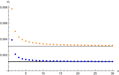
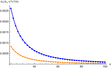
Figure 1: Left: Plot showing that $\sigma_{n}$ decreases monotonically from the entanglement entropy value included for $n=1$ to the asymptotic value $\sigma_{\infty}$ for free scalars (blue) and free Dirac fermions (maize squares). The asymptotic values $\sigma_{\infty}^{(B)}=\tfrac{3\zeta(3)}{32\pi^{4}}\approx 0.0011569$ (black) and $\sigma_{\infty}^{(F)}=\tfrac{\zeta(3)}{4\pi^{4}}\approx 0.00308507$ (gray) are indicated as horizontal lines. Right: The plot illustrates our numerical fit $\sigma_{n}=\sigma_{\infty}\big{(}1+\frac{b_{1}}{n}+\frac{b_{2}}{n^{2}}+\frac{b_{3}}{n^{3}}+\dots\big{)}$, for which we find $b_{1}=b_{2}=b_{3}=1$ for the free scalar, and $b_{1}=1$ and $b_{2}=b_{3}=1-\frac{\pi^{2}}{12\zeta(3)}\approx 0.31578$ for the free fermion; the solid curves are $\frac{b_{2}}{n^{2}}+\frac{b_{3}}{n^{3}}$ for those respective values of $b_{2}$ and $b_{3}$.

As a function of $n$, the Rényi corner coefficient $\sigma_{n}$ decreases monotonically, as shown on the left in figure 1. When $n$ is large, $\sigma_{n}$ asymptotes to a constant value, which we calculate analytically:

$$\boxed{\sigma_{\infty}^{(B)}=\frac{3\zeta(3)}{32\pi^{4}}~{}~{}~{}~{}\text{and}~{}~{}~{}~{}\sigma_{\infty}^{(F)}=\frac{\zeta(3)}{4\pi^{4}}\,.}$$ (1.7)

The appearance of the Riemann zeta-function is intriguing since $\zeta(3)\,\approx 1.20206$ also shows up in the free energies and Rényi entropies for free scalars/fermions on a 3-sphere, as shown by Klebanov, Pufu, Sachdev, and Safdi [9]. Specifically, the free energy of a free real scalar or free fermion on an $n$-covered 3-sphere behaves as $\mathcal{F}_{n}\rightarrow n\mathcal{F}_{\infty}$ for $n\rightarrow\infty$ with

$$\mathcal{F}_{\infty}^{(B)}=\frac{3\zeta(3)}{8\pi^{2}}~{}~{}~{}~{}\text{and}~{}~{}~{}~{}\mathcal{F}_{\infty}^{(F)}=\frac{\zeta(3)}{\pi^{2}}\,.$$ (1.8)

Thus, for both free scalars and fermions we have

$$\sigma_{\infty}^{(B/F)}=\frac{1}{4\pi^{2}}\mathcal{F}_{\infty}^{(B/F)}\,.$$ (1.9)

For finite $n$, there is no apparent relation between $\mathcal{F}_{n}$ and $\sigma_{n}$, however there are some similarities in the subleading large-$n$ behaviors, as we discuss in section 4. The plot on the right in figure 1 shows the large-$n$ behaviors of the Rényi corner coefficients $\sigma_{n}$. A priori it is not clear if there is any relation at large $n$ between $\sigma_{n}$ and $\mathcal{F}_{n}$, but it would be curious to test (1.9) in other examples.

The remainder of the paper details the derivations of the results summarized above. In section 2, we derive the results (1.3) for the entanglement entropy corner coefficient $\sigma$. We then evaluate the Rényi entropy corner coefficients $\sigma_{n}$ in section 3. In section 4, we discuss the asymptotic behavior at large $n$.

2 Evaluation of the EE integrals

In this section we describe the procedure for analytically evaluating the integrals for the coefficients $\sigma^{(B)}$ and $\sigma^{(F)}$ of the entanglement entropy. Our starting point is the integrals [4, 5, 2] presented in equations (B1)-(B3) of [6]. After a change of integration variable from $m$ to $\mu=\sqrt{4m^{2}-1}$, the integrals take the form

$$\begin{split}\sigma^{(B)}&=~{}-\frac{1}{2}\int_{0}^{\infty}d\mu\int_{0}^{\infty}db\,\mu^{2}Ha\left(1-a\right)\frac{\pi}{\cosh^{2}\big{(}\pi b\big{)}}\,,\\ \sigma^{(F)}&=~{}-\int_{0}^{\infty}d\mu\int_{0}^{\infty}db\left[\mu^{2}Ha\left(1-a\right)-\frac{\mu F}{4\pi}\right]\frac{\pi}{\sinh^{2}\big{(}\pi b\big{)}}\,,\end{split}$$ (2.1)

where $a=1/2+ib$ for the scalar and $a=ib$ for the fermion. The functions $H$ and $F$ are defined as

$$H=-\frac{T}{2}\left(\frac{c}{h}X_{1}+\frac{1}{c}X_{2}\right)+\frac{1}{16\pi a\left(a-1\right)}\,,~{}~{}~{}~{}~{}~{}~{}~{}~{}~{}F=-\frac{F_{1}}{F_{2}}\,,$$ (2.2)

with

$$\begin{split}F_{1}&=~{}4\pi chHa\left(1-a\right)\left[\left(2a-1\right)^{2}+\mu^{2}\right]-\frac{1}{4}ch^{2}\left(\mu^{2}+1\right)\,,\\ F_{2}&=~{}\frac{ch\left[\left(2a-1\right)^{2}+\mu^{2}\right]^{2}}{2\left(2a-1\right)\mu}\,.\end{split}$$ (2.3)

The functions $h$, $c$, $X_{1}$, $X_{2}$, and $T$ are defined as follows:

$$h = \frac{2\left(\mu^{2}+(2a-1)^{2}\right)\sin^{2}\left(\pi a\right)}{\left(\mu^{2}+1\right)\left(\cos\left(2\pi a\right)+\cosh\left(\pi\mu\right)\right)}\,,$$

$$c = \frac{2^{2a}\pi a\left(1-a\right)\sec\left(\pi a+\frac{i\pi\mu}{2}\right)\Gamma\!\left(\frac{3}{2}-a+\frac{i\mu}{2}\right)}{\sqrt{\mu^{2}+1}\left(\Gamma\!\left(2-a\right)\right)^{2}\Gamma\!\left(-\frac{1}{2}+a+\frac{i\mu}{2}\right)}\,,$$

$$X_{1} = -\frac{\Gamma\!\left(-a\right)\left[\pi\sinh\left(\frac{\pi\mu}{2}\right)+i\cosh\left(\frac{\pi\mu}{2}\right)\left(\psi\!\left(\frac{1}{2}+a+\frac{i\mu}{2}\right)-\psi\!\left(\frac{1}{2}+a-\frac{i\mu}{2}\right)\right)\right]}{2^{2a+1}\mu\Gamma\!\left(a+1\right)\Gamma\!\left(\frac{1}{2}-a+\frac{i\mu}{2}\right)\Gamma\!\left(\frac{1}{2}-a-\frac{i\mu}{2}\right)\big{(}\cos\left(2\pi a\right)+\cosh\left(\pi\mu\right)\big{)}}\,,$$

$$X_{2} = \big{(}X_{1}\text{ with }a\text{ replaced by }(1-a)\big{)}\,,$$

$$T = \frac{1}{2}\sqrt{h\left[\left(h+1\right)\left(\mu^{2}+1\right)-4a\left(1-a\right)\right]}\,.$$ (2.4)

Here $\psi$ denotes the digamma function, $\psi(z)=\tfrac{d}{dz}\ln\Gamma(z)$.

Our first line of attack involves calculating the quantities $cX_{1}/h$ and $X_{2}/c$ that appear in $H$ in (2.2). Beyond the immediate cancellations that occur in these ratios, one can perform further simplifications using identities involving gamma functions. Namely, one can use the recurrence relation

$$\Gamma\!\left(1+z\right)=z\Gamma\!\left(z\right)$$ (2.5)

and the reflection relation

$$\Gamma\!\left(1-z\right)\Gamma\!\left(z\right)=\frac{\pi}{\sin\left(\pi z\right)}.$$ (2.6)

Surprisingly, all the gamma functions cancel after a series of such substitutions, giving

$$\begin{split}\frac{c}{h}X_{1}&=\frac{\sqrt{\mu^{2}+1}\csc\left(\pi a\right)}{16\pi\mu\left(a-1\right)a}\left[\pi\sinh\left(\tfrac{\pi\mu}{2}\right)+i\cosh\left(\tfrac{\pi\mu}{2}\right)\left(\psi\!\left(\tfrac{1}{2}+a+\tfrac{i\mu}{2}\right)-\psi\!\left(\tfrac{1}{2}+a-\tfrac{i\mu}{2}\right)\right)\right],\\[5.69054pt] \frac{1}{c}X_{2}&=\frac{\sqrt{\mu^{2}+1}\csc\left(\pi a\right)}{16\pi\mu\left(a-1\right)a}\left[\pi\sinh\left(\tfrac{\pi\mu}{2}\right)+i\cosh\left(\tfrac{\pi\mu}{2}\right)\left(\psi\!\left(\tfrac{3}{2}-a+\tfrac{i\mu}{2}\right)-\psi\!\left(\tfrac{3}{2}-a-\tfrac{i\mu}{2}\right)\right)\right].\end{split}$$ (2.7)

It is suggestive that the pre-factors and the form of these two results are the same. We then proceed by adding them together as in (2.2). The linear combination of digamma functions that appears in the result can be simplified using properties easily derived from (2.5) and (2.6). In the form that is useful for our purpose, these identities are

$$\psi\!\left(\tfrac{3}{2}-a\pm\tfrac{i\mu}{2}\right)=\psi\!\left(\tfrac{1}{2}-a\pm\tfrac{i\mu}{2}\right)+\frac{1}{\tfrac{1}{2}-a\pm\tfrac{i\mu}{2}}$$

and

$$\psi\!\left(\tfrac{1}{2}+a\pm\tfrac{i\mu}{2}\right)-\psi\!\left(\tfrac{1}{2}-a\mp\tfrac{i\mu}{2}\right)=\pi\tan\left(\pi a\pm i\tfrac{\pi\mu}{2}\right)\,.$$

Then the combination of $X_{1}$ and $X_{2}$ that appears in $H$ simplifies to

$$\frac{c}{h}X_{1}+\frac{1}{c}X_{2}=\frac{\sqrt{\mu^{2}+1}}{4\pi a(1-a)}\left(\frac{\pi\sin(\pi a)\sinh\left(\frac{\pi\mu}{2}\right)}{\mu\left[\cos(2\pi a)+\cosh(\pi\mu)\right]}-\frac{\csc(\pi a)\cosh\left(\frac{\pi\mu}{2}\right)}{(1-2a)^{2}+\mu^{2}}\right)\,.$$ (2.8)

The last ingredient we need to construct $H$ in (2.2) is $T$. Using (2.4), it is

$$T=\sqrt{\frac{\big{(}(1-2a)^{2}+\mu^{2}\big{)}^{2}\sin^{2}(\pi a)\cosh^{2}\left(\frac{\pi\mu}{2}\right)}{(\mu^{2}+1)\big{(}\cos(2\pi a)+\cosh(\pi\mu)\big{)}^{2}}}\,.$$ (2.9)

Further simplifications of $H$ depend on the nature of variable $a$, as we will see when we specialize to the cases of the free scalar and the free fermion.

Free scalar. To proceed with the evaluation of the integral $\sigma^{(B)}$, we set $a=1/2+ib$ as prescribed for the free scalar. It is furthermore convenient to change integration variable $b\rightarrow b/2$. Using that both $\mu$ and $b$ are positive, the integrand of $\sigma^{(B)}$ simplifies dramatically and becomes

$$\sigma^{(B)}=\int_{0}^{\infty}d\mu\int_{0}^{\infty}db\ \frac{\mu\left[\pi\left(\mu^{2}-b^{2}\right)\sinh(\pi\mu)+2\mu\cosh(\pi b)-2\mu\cosh(\pi\mu)\right]}{64[\cosh(\pi b)-\cosh(\pi\mu)]^{2}}\,.$$ (2.10)

Next, we integrate by parts. Writing

$$\sigma^{(B)}=\frac{1}{64}\int_{0}^{\infty}d\mu\int_{0}^{\infty}db\ \left[\frac{\partial}{\partial\mu}\left(\frac{\mu\left(\mu^{2}-b^{2}\right)}{\cosh\left(\pi b\right)-\cosh\left(\pi\mu\right)}\right)+\frac{b^{2}-\mu^{2}}{\cosh\left(\pi b\right)-\cosh\left(\pi\mu\right)}\right],$$ (2.11)

we see that the boundary term vanishes and we get

$$\sigma^{(B)}=\frac{1}{256}\int_{-\infty}^{+\infty}d\mu\int_{-\infty}^{+\infty}db\ \frac{b^{2}-\mu^{2}}{\cosh\left(\pi b\right)-\cosh\left(\pi\mu\right)}\,.$$ (2.12)

We have extended the limits of integration to facilitate the change of integration variables

$$\mu=x-y~{}~{}~{}~{}\text{and}~{}~{}~{}b=x+y\,.$$ (2.13)

This separates the two integrations and reduces the expression to

$$\sigma^{(B)}=\left(\frac{1}{8}\int_{-\infty}^{+\infty}dx\ \frac{x}{\sinh\left(\pi x\right)}\right)^{2}=\frac{1}{256}\,.$$ (2.14)

This completes the derivation of the result (1.3) for the free scalar.

Free fermion. With $F_{1}$ given in terms of $H$ as in (2.3), we have already done most of the leg-work needed to compute $\sigma^{(F)}$. For the free fermion, we have to take $a=ib$ and it is again convenient to change integration variable $b\rightarrow b/2$. After putting everything together, we have

$$\sigma^{(F)}=-\frac{1}{32}\int_{0}^{\infty}d\mu\int_{0}^{\infty}db\ \frac{\mu\big{[}\pi\left(\mu^{2}-b^{2}-1\right)\sinh(\pi\mu)-2\mu\cosh(\pi b)-2\mu\cosh(\pi\mu)\big{]}}{\left[\cosh(\pi b)+\cosh(\pi\mu)\right]^{2}}\,.$$ (2.15)

We can express the integrand as a total derivative plus remaining terms as

$$\sigma^{(F)}=\frac{1}{32}\int_{0}^{\infty}d\mu\int_{0}^{\infty}db\ \left[\frac{\partial}{\partial\mu}\left(\frac{\mu\left(\mu^{2}-b^{2}-1\right)}{\cosh(\pi b)+\cosh(\pi\mu)}\right)+\frac{1-\mu^{2}+b^{2}}{\cosh(\pi b)+\cosh(\pi\mu)}\right].$$ (2.16)

As before, the boundary term vanishes and we are left with the expression (after extending the limits of integration)

$$\sigma^{(F)}=\frac{1}{128}\int_{-\infty}^{+\infty}d\mu\,db\ \frac{1-\mu^{2}+b^{2}}{\cosh(\pi b)+\cosh(\pi\mu)}=\frac{1}{128}\int_{-\infty}^{+\infty}dx\,dy\,\frac{1+4xy}{\cosh(\pi x)\cosh(\pi y)}\,.$$ (2.17)

In the last step, we changed integration variables using (2.13). Since $x/\cosh(\pi x)$ is odd, that part of the integral vanishes and the result is therefore simply

$$\sigma^{(F)}=\frac{1}{128}\left(\int_{-\infty}^{+\infty}dx\ \frac{1}{\cosh(\pi x)}\right)^{2}=\frac{1}{128}\,.$$ (2.18)

Thus we have derived the result (1.3) for the free fermion.

3 Rényi entropies

We now proceed to calculate the corner coefficients $\sigma_{n}$ for the Rényi entropies.

Free scalar. For the scalar field, the Rényi corner coefficient is given by the integral (B7) in [6]. We change of the integration variable $m$ to $\mu=\sqrt{4m^{2}-1}$ to write it as

$$\sigma_{n}^{(B)}=-\sum_{k=1}^{n-1}\frac{k\left(n-k\right)}{2n^{2}\left(n-1\right)}\int_{0}^{\infty}d\mu\ \mu^{2}H_{k/n}\,,$$ (3.1)

where $H_{k/n}$ is $H$ in (2.2) with $a$ replaced by $k/n$. With the simplified expression for $H$ from section 2, we get

$$\phantom{!}\!\!\!\!\!\!\sigma_{n}^{(B)}=\sum_{k=1}^{n-1}\frac{\sin^{2}\left(\frac{\pi k}{n}\right)}{32\pi n^{2}(n-1)}\int_{0}^{\infty}d\mu\ \frac{\mu\left[(n-2k)^{2}+\mu^{2}n^{2}\right]\pi\sinh(\pi\mu)-2\mu^{2}n^{2}\left[\cos\left(\frac{2\pi k}{n}\right)+\cosh(\pi\mu)\right]}{\left[\cos\left(\frac{2\pi k}{n}\right)+\cosh(\pi\mu)\right]^{2}}\,.$$ (3.2)

As before, we write the integrand as a total derivative plus the remaining terms:

$$\phantom{!}\!\!\!\!\!\!\sigma_{n}^{(B)}=-\sum_{k=1}^{n-1}\frac{\sin^{2}\left(\frac{\pi k}{n}\right)}{32\pi n^{2}(n-1)}\int_{0}^{\infty}d\mu\left[\frac{\partial}{\partial\mu}\left(\frac{\mu\left[(n-2k)^{2}+\mu^{2}n^{2}\right]}{\cos\left(\frac{2\pi k}{n}\right)+\cosh(\pi\mu)}\right)-\frac{(n-2k)^{2}+\mu^{2}n^{2}}{\cos\left(\frac{2\pi k}{n}\right)+\cosh(\pi\mu)}\right]\!.$$ (3.3)

The boundary term vanishes and the expression simplifies to

$$\sigma_{n}^{(B)}=\sum_{k=1}^{n-1}\frac{\sin^{2}\left(\frac{\pi k}{n}\right)}{32\pi n^{2}(n-1)}\int_{0}^{\infty}d\mu\ \frac{(n-2k)^{2}+\mu^{2}n^{2}}{\cos\left(\frac{2\pi k}{n}\right)+\cosh(\pi\mu)}\,.$$ (3.4)

The contribution of $k=n/2$ is easy to calculate and is equal to

$$\frac{1}{64\pi\left(n-1\right)}\int_{0}^{\infty}d\mu\ \frac{\mu^{2}}{\sinh^{2}\left(\frac{\pi\mu}{2}\right)}~{}=~{}\frac{1}{48\pi^{2}\left(n-1\right)}\,.$$ (3.5)

For $k\neq n/2$, there are contributions from two integrals:

$$I^{(1)}_{n;k}=\int_{0}^{\infty}\frac{d\mu}{\cos\left(\frac{2\pi k}{n}\right)+\cosh(\pi\mu)}=\frac{2\tan^{-1}\left(\tan\left(\frac{\pi k}{n}\right)\right)}{\pi\sin\!\big{(}\frac{2k\pi}{n}\big{)}}=\frac{2}{\sin\!\big{(}\frac{2k\pi}{n}\big{)}}\times\left\{\begin{array}[]{ll}\frac{k}{n}\,,&k<n/2\\[2.84526pt] \frac{k}{n}-1\,,&k>n/2\end{array}\right.$$ (3.6)

and

$$I^{(2)}_{n;k} = \int_{0}^{\infty}\frac{\mu^{2}\,d\mu}{\cos\left(\frac{2\pi k}{n}\right)+\cosh(\pi\mu)}=\frac{2i\,\big{[}\operatorname{Li}_{3}\!\big{(}-e^{\frac{2ik\pi}{n}}\big{)}-\operatorname{Li}_{3}\!\big{(}-e^{-\frac{2ik\pi}{n}}\big{)}\big{]}}{\pi^{3}\sin\!\big{(}\frac{2k\pi}{n}\big{)}}$$ (3.7)

$$= -\frac{i\,\log\big{(}e^{\frac{2ik\pi}{n}}\big{)}\big{[}\pi^{2}+\log^{2}\big{(}e^{\frac{2ik\pi}{n}}\big{)}\big{]}}{3\pi^{3}\sin\!\big{(}\frac{2k\pi}{n}\big{)}}=\frac{2}{\sin\!\big{(}\frac{2k\pi}{n}\big{)}}\times\left\{\begin{array}[]{ll}\frac{k(n^{2}-4k^{2})}{3n^{3}}\,,&k<n/2\\[2.84526pt] -\frac{(n-k)(n-2k)(3n-2k)}{3n^{3}}\,,&k>n/2\,.\end{array}\right.$$ (3.10)

Above, we manipulated the tri-logarithm $\operatorname{Li}_{3}$ using the polylog identity

$$\operatorname{Li}_{3}(z)-\operatorname{Li}_{3}\!\big{(}z^{-1}\big{)}=-\frac{1}{6}\log^{3}\left(-z\right)-\frac{\pi^{2}}{6}\log\left(-z\right)\,,$$ (3.11)

which holds for $z\notin\,]0,1[$.

Combining the results (3.6) and (3.7), we find that the result is the same for $1<k<n/2$ and $n/2<k<n$, namely

$$\int_{0}^{\infty}d\mu\ \frac{(n-2k)^{2}+\mu^{2}n^{2}}{\cos\left(\frac{2\pi k}{n}\right)+\cosh(\pi\mu)}~{}=~{}(n-2k)^{2}I^{(1)}_{n;k}+n^{2}I^{(2)}_{n;k}~{}=~{}\frac{8k(n-k)(n-2k)}{3n\,\sin\!\big{(}\frac{2k\pi}{n}\big{)}}\,.$$ (3.12)

Thus, having evaluated the integral in (3.4), we can write $\sigma_{n}^{(B)}$ as the finite sum

$$\sigma_{n}^{(B)}=\frac{1}{24\pi\ n^{3}\left(n-1\right)}\sum_{k=1}^{n-1}k\left(n-k\right)\left(n-2k\right)\tan\!\left(\tfrac{\pi k}{n}\right)\,.$$ (3.13)

Note that taking the limit $k\rightarrow n/2$ as described below (1.5), the summand evaluates precisely to the special case (3.5). The expression (3.13) is the result for the Rényi corner coefficient presented in (1.5), so this completes our evaluation for the free scalar.

Free fermion. For the fermion field, the Rényi corner coefficient is given by the integral

$$\sigma_{n}^{(F)}=-\frac{2}{n-1}\sum_{k>0}^{\frac{1}{2}(n-1)}\int_{0}^{\infty}d\mu\ \left[a\left(1-a\right)\mu^{2}H-\frac{\mu F}{4\pi}\right]_{a=k/n}\,,$$ (3.14)

where the sum is over $k$ from $1/2$ ($n$ even) or $1$ ($n$ odd) in integer steps to $\frac{1}{2}(n-1)$. Substituting the expressions for $H$ and $F$ obtained earlier gives

$$\sigma_{n}^{(F)}=\sum_{k>0}^{\frac{1}{2}(n-1)}\frac{\sin^{2}\left(\frac{\pi k}{n}\right)}{8\pi(n-1)}\int_{0}^{\infty}d\mu\ \frac{2\mu^{2}\left[\cos\left(\frac{2\pi k}{n}\right)+\cosh(\pi\mu)\right]-\mu\left(\frac{4k^{2}}{n^{2}}+\mu^{2}-1\right)\pi\sinh(\pi\mu)}{\left[\cos\left(\frac{2\pi k}{n}\right)+\cosh(\pi\mu)\right]^{2}}\,.$$ (3.15)

We then use integration by parts to simplify the integral

$$\sigma_{n}^{(F)}=\sum_{k>0}^{\frac{1}{2}(n-1)}\frac{\sin^{2}\left(\frac{\pi k}{n}\right)}{8\pi(n-1)}\int_{0}^{\infty}d\mu\ \left[\frac{\partial}{\partial\mu}\left(\frac{\mu\left(\frac{4k^{2}}{n^{2}}+\mu^{2}-1\right)}{\cos\left(\frac{2\pi k}{n}\right)+\cosh(\pi\mu)}\right)-\frac{\frac{4k^{2}}{n^{2}}+\mu^{2}-1}{\cos\left(\frac{2\pi k}{n}\right)+\cosh(\pi\mu)}\right].$$ (3.16)

The boundary term integrates to zero and the expression simplifies to

$$\sigma_{n}^{(F)}=\sum_{k>0}^{\frac{1}{2}(n-1)}\frac{\sin^{2}\left(\frac{\pi k}{n}\right)}{8\pi(n-1)}\int_{0}^{\infty}d\mu\ \frac{1-\mu^{2}-\frac{4k^{2}}{n^{2}}}{\cos\left(\frac{2\pi k}{n}\right)+\cosh(\pi\mu)}\,.$$ (3.17)

The result of the integral again involves a difference of two tri-logarithms and it can be simplified using equation (3.11). The result is even in $k\rightarrow-k$ and we can write the final answer as

$$\sigma_{n}^{(F)}=\frac{1}{24\pi\ n^{3}\left(n-1\right)}\sum_{k=-\frac{1}{2}(n-1)}^{\frac{1}{2}(n-1)}k\left(n^{2}-4k^{2}\right)\tan\left(\frac{\pi k}{n}\right).$$ (3.18)

This is the answer we presented in (1.6). Values for low $n$ were tabulated in section 1 for both $\sigma_{n}^{(B)}$ and $\sigma_{n}^{(F)}$.

4 Asymptotic behavior of the Rényi’s

Let us now study the large $n$ behavior of the Rényi entropy corner coefficients $\sigma_{n}$. In particular, we evaluate analytically the value for the coefficients $\sigma_{n}$ in the limit where $n\rightarrow\infty$. This is done by introducing a new variable $x=k/n$ and multiplying by $n\Delta x=1$. Then in the $n\rightarrow\infty$ limit, the sum becomes an integral and we have

$$\begin{split}\sigma_{\infty}^{(B)}&=~{}\frac{1}{24\pi}\int_{0}^{1}dx\ x\left(x-1\right)\left(2x-1\right)\tan\left(\pi x\right)=\frac{3\zeta(3)}{32\pi^{4}}\,,\\[5.69054pt] \sigma_{\infty}^{(F)}&=~{}\frac{1}{24\pi}\int_{-1/2}^{1/2}dx\ x\left(1-4x^{2}\right)\tan\left(\pi x\right)=\frac{\zeta(3)}{4\pi^{4}}\,.\end{split}$$ (4.1)

These values turn out to be proportional to the asymptotic values of the $\mathcal{F}_{n}\rightarrow n\mathcal{F}_{\infty}$ calculated on the $n$-covered 3-sphere [9]; as noted in (1.9) we have $\sigma_{\infty}^{(B/F)}=\frac{1}{4\pi^{2}}\mathcal{F}_{\infty}^{(B/F)}$.

On the right in figure 1, we illustrated the asymptotic behavior of the corner coefficient which we find to be

$$\sigma_{n}=\sigma_{\infty}\Big{(}1+\frac{b_{1}}{n}+\frac{b_{2}}{n^{2}}+\frac{b_{3}}{n^{3}}+\dots\Big{)}\,.$$ (4.2)

Numerical fits show that $b_{1}$, $b_{2}$, and $b_{3}$ are $1$ for the free boson while $b_{1}$ is $1$ and $b_{2}=b_{3}\approx 0.31578$ in (4.2) for the free fermion. In fact, fitting up to $O(1/n^{16})$, we find numerical evidence that $b_{2k}=b_{2k+1}$ for both the scalar and fermion. This indicates that a factor of $(n+1)/n$ can be factored out of the function in (4.2), so that

$$\sigma_{n}=\sigma_{\infty}\frac{n+1}{n}\Big{(}1+\frac{b_{2}}{n^{2}}+\frac{b_{4}}{n^{4}}+\frac{b_{6}}{n^{6}}+\dots\Big{)}\,.$$ (4.3)

It is also interesting to study the ratios of the Rényi corner coefficients at large $n$: based on numerical fits in the range $n=100$ to $2000$ we find

$$\frac{\sigma_{n}^{(B)}}{\sigma_{n}^{(F)}}=\frac{3}{8}\Big{[}1+\frac{\pi^{2}}{12\zeta(3)}\frac{1}{n^{2}}-0.93871149\frac{1}{n^{4}}+O\Big{(}\frac{1}{n^{5}}\Big{)}\Big{]}\,.$$ (4.4)

The value of the $1/n^{2}$-coefficient is guessed based on the numerics. Specifically, we fit to the function

$$\frac{3}{8}\Big{(}1+\frac{d_{1}}{n}+\frac{d_{2}}{n^{2}}+\frac{d_{3}}{n^{3}}+\dots\Big{)}\,,$$ (4.5)

and find that $d_{1}<10^{-26}$, $\big{|}d_{2}-\frac{\pi^{2}}{12\zeta(3)}\big{|}<10^{-23}$, $d_{3}<10^{-19}$, $d_{4}=-0.93871149\dots$, $d_{5}<10^{-13}$ etc. The vanishing of the odd powers in (4.5) is consistent with (4.3). Note also that we can now identify the number $b_{2}=b_{3}\approx 0.31578$ from the fit (4.2) of the free fermion Rényi entropy corner coefficient at large $n$ as $1-\tfrac{\pi^{2}}{12\zeta(3)}$; this is the value given in the caption of figure 1.

Taking the Hurwitz zeta-function expressions for $\mathcal{F}_{n}^{(B/F)}$ from [9] and using (4.5) to perform a similar fit at large $n$ in the range $30$ to $300$, we find

$$\frac{\mathcal{F}_{n}^{(B)}}{\mathcal{F}_{n}^{(F)}}=\frac{3}{8}\Big{[}1-\frac{\pi^{2}}{12\zeta(3)}\frac{1}{n^{2}}+0.937106586\frac{1}{n^{4}}+O\Big{(}\frac{1}{n^{5}}\Big{)}\Big{]}\,.$$ (4.6)

Again, the value of the $1/n^{2}$-coefficient is guessed based on the numerics which give $d_{1}<10^{-20}$, $\big{|}d_{2}+\frac{\pi^{2}}{12\zeta(3)}\big{|}<10^{-17}$, $d_{3}<10^{-14}$, $d_{4}=0.937106586\dots$, $d_{5}<10^{-12}$ etc. The behaviors of $\mathcal{F}_{n}^{(B/F)}$ individually is, however, very different that that of the Rényi corner coefficients. We find that $\mathcal{F}_{n}^{(B)}\sim n\mathcal{F}_{\infty}^{(B)}\big{(}1+O(\tfrac{1}{n^{4}})\big{)}$ while $\mathcal{F}_{n}^{(F)}\sim n\mathcal{F}_{\infty}^{(F)}\big{(}1+\tfrac{\pi^{2}}{12\zeta(3)}\tfrac{1}{n^{2}}+O(\tfrac{1}{n^{4}})\big{)}$.

It is not clear whether the similarities observed at large $n$ between $\sigma_{n}$ and $\mathcal{F}_{n}$ have any significance or if it is a coincidence. Perhaps future investigations will clarify this.

References

[1]
E. Fradkin and J. E. Moore,
“Entanglement entropy of 2D conformal quantum critical points: hearing the shape of a quantum drum,”
Phys. Rev. Lett. 97, 050404 (2006)
[cond-mat/0605683 [cond-mat.str-el]].
[2]
H. Casini and M. Huerta,
“Universal terms for the entanglement entropy in 2+1 dimensions,”
Nucl. Phys. B 764, 183 (2007)
[hep-th/0606256].
[3]
T. Hirata and T. Takayanagi,
“AdS/CFT and strong subadditivity of entanglement entropy,”
JHEP 0702, 042 (2007)
[hep-th/0608213].
[4]
H. Casini, M. Huerta and L. Leitao,
“Entanglement entropy for a Dirac fermion in three dimensions: Vertex contribution,”
Nucl. Phys. B 814, 594 (2009)
[arXiv:0811.1968 [hep-th]].
[5]
H. Casini and M. Huerta,
“Entanglement entropy in free quantum field theory,”
J. Phys. A 42, 504007 (2009)
[arXiv:0905.2562 [hep-th]].
[6]
P. Bueno, R. C. Myers and W. Witczak-Krempa,
“Universality of corner entanglement in conformal field theories,”
arXiv:1505.04804 [hep-th].
[7]
P. Bueno and R. C. Myers,
“Corner contributions to holographic entanglement entropy,”
arXiv:1505.07842 [hep-th].
[8]
H. Osborn and A. C. Petkou,
“Implications of conformal invariance in field theories for general dimensions,”
Annals Phys. 231, 311 (1994)
[hep-th/9307010].
[9]
I. R. Klebanov, S. S. Pufu, S. Sachdev and B. R. Safdi,
“Renyi Entropies for Free Field Theories,”
JHEP 1204, 074 (2012)
[arXiv:1111.6290 [hep-th]].