The Distribution and Annihilation of Dark Matter Around Black Holes

Abstract

We use a Monte Carlo code to calculate the geodesic orbits of test particles around Kerr black holes, generating a distribution function of both bound and unbound populations of dark matter particles. From this distribution function, we calculate annihilation rates and observable gamma-ray spectra for a few simple dark matter models. The features of these spectra are sensitive to the black hole spin, observer inclination, and detailed properties of the dark matter annihilation cross section and density profile. Confirming earlier analytic work, we find that for rapidly spinning black holes, the collisional Penrose process can reach efficiencies exceeding $600\%$, leading to a high-energy tail in the annihilation spectrum. The high particle density and large proper volume of the region immediately surrounding the horizon ensures that the observed flux from these extreme events is non-negligible.

1. INTRODUCTION

Prompted by the recent paper by Bañados et al. (2009) [BSW], there has been a great deal of interest in the potential of Kerr black holes to accelerate particles to ultra-relativistic energies and thus to probe a regime of physics otherwise inaccessible. The vast majority of this work has been analytic and thus largely limited to the most simple photon and particle trajectories in the equatorial plane. Here we present a more numerical approach that focuses on calculating the fully relativistic distribution function of massive test particles around a spinning black hole. With this distribution function and a simple model for the dark matter annihilation mechanism, we can then calculate the annihilation rate and observed spectrum as a function of black hole spin and observer inclination.

It has been noted repeatedly in recent works that the net energy gained through the Penrose process is quite modest, as is the fraction of collision products that might escape, and thus the astrophysical importance of the BSW effect is questionable (Jacobson & Sotiriou, 2010; Bañados et al., 2011; Harada et al., 2012; Bejger et al., 2012; McWilliams, 2013). We argue here that two primary factors (to our knowledge largely neglected in previous work) could greatly enhance the astrophysical relevance and observability of this annihilation. The first is an energy-dependent cross section for dark matter (DM) annihilation. This could take many forms, the simplest of which are p-wave annihilation (Bertone et al., 2005; Chen & Zhou, 2013; Ferrer & Hunter, 2013), where the cross section scales like the relative velocity, or a threshold energy, above which the cross section increases greatly. This latter assumption is a natural choice for a model that includes multiple DM species, with the more massive particles intermediate products in the annihilation process towards gamma rays [see, e.g., Zurek (2014)]. Because gravity is the only known force capable of accelerating dark matter particles to high energies, it is possible that new annihilation channels could occur around black holes that are completely inaccessible everywhere else in the universe.

The other effect considered here is the relativistic enhancement of the density close to the black hole. This is due to the time dilation of observers near the horizon. In a steady-state system, one can think of dropping particles into the black hole from infinity at a constant rate $\Gamma_{\infty}$ as measured by coordinate time $t$. To an observer near the black hole measuring proper time $\tau$, an enhanced rate $\Gamma_{\infty}(dt/d\tau)$ is seen, with $dt/d\tau>1$. For annihilation rates that scale like the density squared, the local annihilation rate will be enhanced by $(dt/d\tau)^{2}$. Of course, the products will get redshifted on their way back out to an observer at infinity (McWilliams, 2013), but we are still left with a net enhancement of $dt/d\tau$.

Even without this relativistic enhancement, numerous models also predict an astrophysical enhancement of the dark matter density in the galactic nucleus. Adiabatic growth of the central black hole will capture a large number of particles onto tightly bound orbits, growing a steep density spike as the black hole grows (Gondolo & Silk, 1999; Sadeghian et al., 2013). Gravitational scattering off the dense nuclear star cluster will also lead to a dark matter spike (Gnedin & Primack, 2004), similar to the classical two-body scattering result of Bahcall & Wolf (1976). At the same time, self-annihilation (Gondolo & Silk, 1999) and elastic scattering (Shapiro & Paschalidis, 2014; Fields et al., 2014) will act to flatten out this spike into a shallow core more similar to the unbound population.

Because our approach to this problem is predominantly numerical, we can easily include treatment of a range of black hole spins, particle distributions, and cross sections, and not limit ourselves to special cases with analytic solutions. Therefore, we can calculate how often those extreme cases are likely to occur in a real astrophysical setting [for a notable exception to the analytic approaches of earlier work, see the exhaustive Monte Carlo calculations of Williams (1995, 2004) that explored the limits of the Penrose process in the context of Compton scattering and pair production in accretion disks and jets]. Of particular interest has been the following question: for two particles each of mass $m_{\chi}$ falling from rest at infinity and colliding near the black hole, what is the maximum achievable energy for an escaping photon? We find that this limit exceeds $12m_{\chi}$ for an extremal black hole with $a/M=1$, significantly higher than previously published values of $2.6m_{\chi}$ (Bejger et al., 2012). We explain the underlying reason for this discrepancy in a companion paper (Schnittman, 2014).

2. POPULATING THE DISTRIBUTION FUNCTION

2.1. Initial conditions

The primary goal of this paper is to calculate the 8-dimensional phase-space distribution function $df(\mathbf{x},\mathbf{p})$ of DM particles around a Kerr black hole. Two of these dimensions are immediately removed due to the assumption of a steady-state solution and stationarity of the metric, and the mass-shell constraint of the particle momentum, leaving us with $df(r,\theta,\phi,p_{r},p_{\theta},p_{\phi})$. This function is further reduced to five dimensions because axisymmetry removes the dependence on $\phi$.

To calculate the distribution function, we first distinguish between two basic populations: the particles gravitationally bound and unbound to the black hole. The properties of the bound populations are more sensitive to underlying astrophysical assumptions, and will be discussed below in Section 2.4. The unbound population is more straightforward: we simply assume an isotropic, thermal distribution of velocities at a large distance from the black hole. Here, “large distance” is taken to be the influence radius $r_{\rm infl}$ of a supermassive black hole with mass $M$, and the DM velocity dispersion is set equal to the stellar velocity dispersion $\sigma_{0}$ of the bulge (thus the “unbound” population considered in this paper is still gravitationally bound to the galaxy, just not the black hole). From the “M-sigma” relation (Ferrarese & Merritt, 2000) we take

$$M\approx 2\times 10^{7}M_{\odot}\left(\frac{\sigma_{0}}{100\mbox{ km/s}}\right)^{4}$$ (1)

and

$$r_{\rm infl}\equiv\frac{GM}{\sigma_{0}^{2}}\approx 8\mbox{ pc}\left(\frac{\sigma_{0}}{100\mbox{ km/s}}\right)^{2}\,.$$ (2)

In units of gravitational radii $r_{g}=GM/c^{2}$, the influence radius is typically quite large: $r_{\rm infl}\approx 10^{7}M_{7}^{-1/2}r_{g}$, where $M_{7}\equiv(M/10^{7}M_{\odot})$.

Given this outer boundary condition, we shoot test particles towards the black hole with initial velocities drawn from an isotropic thermal distribution with characteristic velocity $\sigma_{0}$. As we are only interested in the distribution function relatively close to the black hole, we can ignore any particle with impact parameter greater than $\approx 1000\,r_{g}$. For those particles that we do follow, we calculate their geodesic trajectories with the Hamiltonian approach described in detail in Schnittman & Krolik (2013) and used in the radiation transport code Pandurata. A schematic of this procedure is shown in Figure 1. As the particle moves around the black hole and passes through different finite volume elements, the discretized distribution function $df(r_{i},\theta_{j},\mathbf{p})$ is updated with appropriate weights.

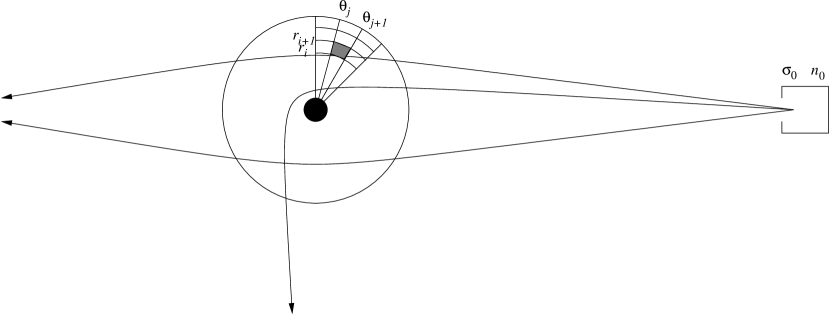
Figure 1.— Schematic of our method for populating phase space with geodesic trajectories. The test particles are injected at large radius ($r_{0}=10^{7}r_{g}$) with thermal velocities with dispersion $\sigma_{0}\ll c$. Those particles passing within $1000\,r_{g}$ of the black hole contribute to the tabulated distribution function in each volume element $(r_{i},\theta_{j})$ through which they pass, with a weight proportional to the amount of coordinate time $t$ spent in that zone.

The great advantage of this Hamiltonian approach is that the integration variable is the coordinate time $t$ in Boyer-Lindquist coordinates (Boyer & Lindquist, 1967). Because this is the time measured by an observer at infinity, it determines the rate at which particles are injected into the system in the steady-state limit. Then the distribution function can be populated numerically by assigning a weight to each bin in phase space through which the test particle passes, with the weight proportional to the amount of time $t$ spent in that volume. The process is repeated for many Monte Carlo test particles until the 5-dimensional distribution function is completely populated.

2.2. Geodesics and Tetrads

Following Schnittman & Krolik (2013), we define local orthonormal observer frames, or tetrads, at each point in the computational volume. Depending on the population in question (i.e., bound vs. unbound), it is convenient to use either the zero-angular-momentum observer (ZAMO; Bardeen et al. (1972)) or the “free-falling from infinity observer” (FFIO) tetrads. In all cases we use Boyer-Lindquist coordinates (Boyer & Lindquist, 1967), where the metric can be written

$$g_{\mu\nu}=\begin{pmatrix}-\alpha^{2}+\omega^{2}\varpi^{2}&0&0&-\omega\varpi^{2}\\ 0&\rho^{2}/\Delta&0&0\\ 0&0&\rho^{2}&0\\ -\omega\varpi^{2}&0&0&\varpi^{2}\end{pmatrix}\,.$$ (3)

This allows for a relatively simple form for the inverse metric:

$$g^{\mu\nu}=\begin{pmatrix}-1/\alpha^{2}&0&0&-\omega/\alpha^{2}\\ 0&\Delta/\rho^{2}&0&0\\ 0&0&1/\rho^{2}&0\\ -\omega/\alpha^{2}&0&0&1/\varpi^{2}-\omega^{2}/\alpha^{2}\end{pmatrix}\,,$$ (4)

with the following definitions:

$$\rho^{2} \equiv r^{2}+a^{2}\cos^{2}\theta$$ (5a)

$$\Delta \equiv r^{2}-2Mr+a^{2}$$ (5b)

$$\alpha^{2} \equiv \frac{\rho^{2}\Delta}{\rho^{2}\Delta+2Mr(a^{2}+r^{2})}$$ (5c)

$$\omega \equiv \frac{2Mra}{\rho^{2}\Delta+2Mr(a^{2}+r^{2})}$$ (5d)

$$\varpi^{2} \equiv \left[\frac{\rho^{2}\Delta+2Mr(a^{2}+r^{2})}{\rho^{2}}\right]\sin^{2}\theta\,.$$ (5e)

Unless explicitly included, we adopt units with $G=c=1$, so distances and times are often scaled by the black hole mass $M$.

The ZAMO tetrad can be constructed by

$$\mathbf{e}_{(\tilde{t})} = \frac{1}{\alpha}\mathbf{e}_{(t)}+\frac{\omega}{\alpha}\mathbf{e}_{(\phi)}$$ (6a)

$$\mathbf{e}_{(\tilde{r})} = \sqrt{\frac{\Delta}{\rho^{2}}}\mathbf{e}_{(r)}$$ (6b)

$$\mathbf{e}_{(\tilde{\theta})} = \sqrt{\frac{1}{\rho^{2}}}\mathbf{e}_{(\theta)}$$ (6c)

$$\mathbf{e}_{(\tilde{\phi})} = \sqrt{\frac{1}{\varphi^{2}}}\mathbf{e}_{(\phi)}\,,$$ (6d)

where we designate tetrad basis vectors by $\tilde{\mu}$ indices, while coordinate bases have normal indices.

To construct the FFIO tetrad, the time-like basis vector $\mathbf{e}_{(\tilde{t})}$ is given by the 4-velocity $u^{\mu}=g^{\mu\nu}u_{\nu}$ corresponding to a geodesic with $u_{t}=-1$, $u_{\theta}=u_{\phi}=0$, and from normalization constraints,

$$u_{r}=-\left[(\alpha^{-2}-1)\frac{\rho^{2}}{\Delta}\right]^{1/2}\,.$$ (7)

Then the spatial basis vectors $\mathbf{e}_{(\tilde{i})}$ are constructed via a standard Gram-Schmidt method and aligned roughly parallel to the Boyer-Lindquist coordinate bases.

Any vector can be represented by its components in different tetrads via the relation

$$\mathbf{u}=\mathbf{e}_{(\mu)}u^{\mu}=\mathbf{e}_{(\tilde{\mu})}u^{\tilde{\mu}}\,,$$ (8)

whereby the components are related by a linear transformation $E_{\tilde{\mu}}^{\mu}$:

$$u^{\mu} = E_{\tilde{\mu}}^{\mu}u^{\tilde{\mu}}\,,$$ (9a)

$$u^{\tilde{\mu}} = [E^{-1}]_{\mu}^{\tilde{\mu}}u^{\mu}\,.$$ (9b)

These $u^{\tilde{\mu}}$ are the components that we use for the tabulated distribution function. Because of the normalization constraints, we need only store three components of the 4-momentum in each spatial volume element, making the total dimensionality of the distribution function five: two space and three momentum.

In Pandurata, the geodesics are integrated with a variable time step 5^th order Cash-Karp algorithm (Schnittman & Krolik, 2013). This technique very naturally matches small time steps to regions of high curvature and thus areas of high resolution in the spatial grid. For each time step, a weight proportional to the coordinate time spent on that step is added to the distribution function for that particular volume of phase space. Because the particle typically remains within a single volume element for many time steps, we find that interpolation errors are small.

The spatial momentum components $\gamma\beta^{\tilde{i}}$ can be positive or negative and span many orders of magnitude. To adequately resolve the phase space and capture the relativistic effects immediately outside the black hole horizon, we find that on order $\sim 10^{3}$ bins are required in each dimension. If the entire phase-space volume were occupied, this would correspond to an unfeasible quantity of data. Fortunately, this volume is not evenly filled, so such a hypothetical 5-dimensional array is in fact exceedingly sparse. In practice, we are able to use a dynamic memory allocation technique that only stores the non-zero elements of the distribution function. Yet even so, a well-resolved calculation can easily require multiple GB of data for a single distribution function, and to adequately sample this phase space requires on the order of $\sim 10^{9}$ test particles, with each geodesic sampled over thousands of time steps. Fortunately, this is a trivially parallelizable problem, so it is relatively simple to achieve sufficient resolution in a reasonable amount of time with a small computer cluster.

2.3. Unbound Particles

As mentioned above, for the unbound population, the outer boundary condition for the phase space density at $r_{\rm infl}$ is relatively well-understood. The velocity distribution is thermal with characteristic speed $\sigma_{0}$. The spatial density of dark matter is measured from galactic rotation curves at kpc distances from the nucleus, and then must be extrapolated in to pc distances with a combination of observations and stellar profile modeling. For example, in the Milky Way the DM density near the Sun is 0.3 GeV/cm³, and the radial profile can be reasonably well-modeled with a simple $\rho\sim R^{-1}$ profile, giving a density of $\sim 10^{3}$ GeV/cm³ at $r_{\rm infl}$. Inside of $r_{\rm infl}$ there is almost certainly an additional bound component to the DM distribution (Gondolo & Silk, 1999), so the unbound population described here can best be understood as a strict lower bound on the phase space density.

Outside of $\sim 100\,r_{g}$ the unbound population can be treated as a collisionless gas of accreting particles, as in Zeldovich & Novikov (1971). In the Newtonian limit, the density and velocity dispersion can be written

$$n(r)=n_{0}\left(1+\frac{2GM}{\sigma_{0}^{2}r}\right)^{1/2}$$ (10)

and

$$\sigma^{2}(r)=\sigma_{0}^{2}\left(1+\frac{2GM}{\sigma_{0}^{2}r}\right)\,.$$ (11)

Figure 2.— Spatial density (a) and mean relative momentum $\langle\gamma\beta\rangle_{\rm rel}$ (b) of unbound particles as measured in the FFIO frame in the equatorial plane of a Kerr black hole with $a/M=1$. The dashed lines are the Newtonian solutions of equations (10, 11), while the solid curves come from the fully relativistic Monte Carlo calculation.

In Figure 2 we show the spatial density of unbound particles as measured by a FFIO around a Kerr black hole with spin parameter $a/M=1$, as well as the mean particle momentum as measured in that frame. We find very close agreement to the Newtonian results all the way down to $r\sim 10r_{g}$. The deviation of the momentum from the Newtonian solution is due largely to the special relativistic terms proportional to the Lorentz boost $\gamma$.

The proper density is governed by two competing relativistic effects. One is time dilation and the other is spatial curvature. Close to the black hole, the particle’s proper time $\tau$ slows down relative to the coordinate time $t$ measured by an observer at infinity, giving a large $dt/d\tau$. This has the effect of increasing the number density because, in a steady state, particles are injected into the system at a constant rate—as measured by an observer at infinity. The injection rate measured by an observer close to the black hole is higher by a factor of $dt/d\tau$, leading to her seeing a larger proper density.

Figure 3.— Proper volume measured in the FFIO frame. The dashed line is the Newtonian value $dV/dr=4\pi r^{2}$, and the solid curve measures the FFIO’s proper volume $d\tilde{V}/dr$.

In fact, the proper density would be even higher if it weren’t for another important relativistic effect: the stretching of space around a black hole. Specifically, the Boyer-Lindquist radial coordinate element $dr$ corresponds to a greater and greater proper distance as the observer approaches the horizon. This naturally gives a greater proper volume $d\tilde{V}$, shown as a solid curve in Figure 3. Again, we show the Newtonian value $dV/dr=4\pi r^{2}$ as a dashed curve. Because the particle interaction rates scale like $n^{2}\,v\,d\tilde{V}$, all these effects combine to increase the importance of reactions near the black hole.

Figure 4.— Momentum distribution of unbound particles observed by a FFIO in the equatorial plane at radius $r=100M$. All particles have nearly unitary specific energy at infinity, so the average particle speed is very close to $\sqrt{2GM/r}=\sqrt{0.02}c$ (panel a). In panels (b-d) we show the distribution of the individual momentum components, which are nearly isotropic this far from the black hole.

In Figure 4 we plot the momentum distributions of unbound dark matter particles, as observed by a FFIO in the equatorial plane, at a relatively large distance from the black hole: $r=100M$. Each 1-dimensional distribution is calculated by integrating over the other two momentum dimensions. We also plot the momentum magnitude $\gamma|\beta|$ in panel (a). Because the particles all have relatively small velocities at infinity $\beta_{0}\approx\sigma_{0}/c\ll 1$, their velocities in the weakly relativistic region $r_{g}\ll r\ll r_{0}$ are given by $v\approx\sqrt{2GM/r}$, corresponding to $v\approx 0.14c$ for $r=100M$.

For the three spatial components of the momentum distribution, we see a nearly isotropic velocity distribution with a few subtle but interesting deviations. First, we note how there is a slight deficit of particles with positive $p^{\tilde{r}}$. This is due to capture by the black hole of particles coming in from infinity with nearly radial trajectories. By definition, these particles also have small values of $p^{\tilde{\theta}}$ and $p^{\tilde{\phi}}$, depleting the distribution function in those dimensions around $\beta=0$. While the distribution in the $\theta$ dimension is symmetric, note that the depletion in the $\phi$ distribution is offset to slightly negative values of $p^{\tilde{\phi}}$. This is due to the well-known preferential capture by Kerr black holes of retrograde particles with angular momenta aligned opposite to the black hole spin.

Figure 5.— Momentum distribution of unbound particles observed by a FFIO in the equatorial plane at radius $r=2M$. Unlike Figure 4, here we see a decidedly non-thermal and highly anisotropic distribution.

In Figure 5, we plot the phase-space distribution for the same boundary conditions as in Figure 4, but now at $r=2M$. The difference is quite dramatic, but all the features are essentially due to the same physical mechanisms. This close to the horizon, there is a very strong depletion of outgoing particles with $p^{\tilde{r}}>0$, as most particles are captured by the black hole. The only particles that can avoid capture at this radius have prograde trajectories in the equatorial plane. Thus, the distribution is now peaked around $p^{\tilde{\theta}}=0$ instead of showing a deficit.

There is also a strong peak near $p^{\tilde{\phi}}=1$ due to the relatively stable, long-lived prograde orbits that circle the black hole multiple times before getting captured or escaping back out to infinity. In fact, the distribution of coordinate momentum is significantly more lopsided to $p^{\phi}>0$, but this is masked in Figure 5d because this distribution is measured by an observer with $u^{\phi}>0$ herself. The sharp fall-off of the azimuthal distribution above $p^{\tilde{\phi}}\approx 1$ is due to the angular momentum barrier of the black hole. Particles with higher values of $p^{\tilde{\phi}}$ simply never reach this small radius.

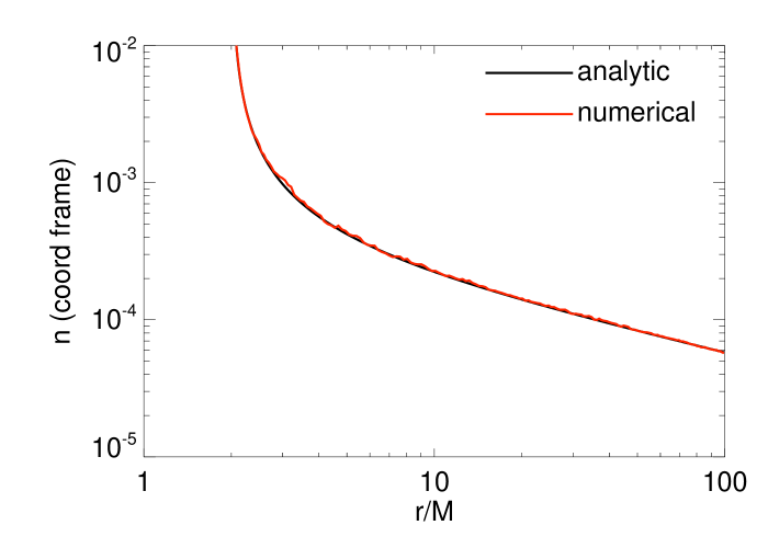
Figure 6.— Comparison of our numerical results (red) with the analytic expression (black) for the particle density derived by Baushev (2009) for a Schwarzschild black hole. The density here is defined in the coordinate, not proper, frame, leading to a much steeper rise at small $r$. In Boyer-Lindquist coordinates, the horizon for a non-spinning black hole is at $r=2M$.

To the best of our knowledge, these distribution functions have never been calculated before for a Kerr black hole. However, the particle number density can be determined analytically for a non-spinning Schwarzschild black hole, in the limit of $\sigma_{0}\ll c$. This allows at least one test of our numerical methods, although admittedly not a very strong one, as most of the interesting features are related to the far more complicated orbits around a spinning black hole. We follow the approach of Baushev (2009), who integrates the distribution function with fixed energy, carefully setting the angular momentum integration bounds based on which orbits are captured from a given radius. The results are shown in Figure 6, with our numerical calculation plotted as a red curve and the analytic result in black, showing perfect agreement. Note that Baushev’s expression is given for a coordinate density rather than a proper density, which also explains the sharper peak at small $r$.

2.4. Bound Particles

As mentioned above, the unbound population can be thought of as a lower limit on the total DM density. There will also likely be a substantial population of particles that are gravitationally bound to the black hole. As described in Gondolo & Silk (1999), the origin of the bound population is the adiabatic growth of the supermassive black hole on a timescale much longer than the typical orbital time. This physical mechanism can be understood as follows: as a marginally unbound DM particle passes within $r_{\rm infl}$, a small amount of baryonic matter is accreted into this region, deepening the potential well just enough to capture the particle onto a marginally bound orbit. Once captured, the particle continues to orbit the black hole while conserving its orbital angular momentum as the black hole continues to gain mass. This has the effect of shrinking the radius of the orbit.

Over time, more particles are captured and subsequently migrate closer to the black hole, building up a steep density spike (Gondolo & Silk, 1999). Inside of the inner-most stable circular orbit (ISCO), there is a sharp falloff in the density spike due to plunging trajectories (Sadeghian et al., 2013). Here we do not attempt to solve for the slope of the density spike at large radii but leave it as a free parameter, and fix the density at the influence radius as for the unbound population: $n_{\rm bound}(r)=n_{0}(r/r_{0})^{-\alpha}$. Following Gondolo & Silk (1999), we also allow for the possibility of a density upper bound $n_{\rm annih}$ due to annihilation losses occurring over very long timescales.

To populate the phase-space distribution for the bound population, we follow a similar method as described above for the unbound particles, but instead of launching them from large radius with a limited range of impact parameters, now we launch them in situ with a isotropic thermal velocity distribution, as measured by a local ZAMO. These particles begin much closer to the black hole, so the relativistic Maxwell-Jüttner velocity distribution is used (Jüttner, 1911), with the characteristic virial temperature $\Theta(r)=1/2[1-\epsilon_{\rm ZAMO}(r)]$, where $\epsilon_{\rm ZAMO}(r)-1$ is the specific gravitational binding energy of the ZAMO.

Because many of the particles launched close to the black hole get captured, we first integrate their trajectories for a few orbital periods to ensure they are in fact on stable orbits. Only then do they contribute to the tabulated distribution function. Additionally, a small fraction of the test particles from the tail end of the velocity distribution will in fact be unbound, and these are similarly discarded.

As with the unbound distribution, for each step along its trajectory, the test particle contributes to the phase space distribution a small weight proportional to the amount of time spent on that step. Yet now, instead of using the coordinate time $dt$, we use the proper time of the ZAMO frame from which the particles are launched, including an additional weight to ensure the appropriate radial form of the density distribution at larger radii.

Figure 7.— Spatial density (a) and mean relative momentum $\langle\gamma\beta\rangle_{\rm rel}$ (b) of bound particles in the equatorial plane of a Kerr black hole with $a/M=1$, as measured in the ZAMO frame. The dashed lines are the Newtonian solutions when $n(r)\sim r^{-2}$ far from the black hole.

In Figure 7 we plot the radial density distribution and mean relative momentum of the bound particles, as measured in the ZAMO frame, in the equatorial plane around a Kerr black hole with spin $a/M=1$. The density profile is constructed so that $\rho(r)\sim r^{-2}$ at large radii. We clearly see major differences relative to the unbound population shown in Figure 2. Because of the lack of stable orbits close to the black hole, the bound population declines inside $r\approx 4M$, which corresponds roughly to the mean radius of the ISCO for randomly inclined orbits around a maximally spinning black hole. This effect was described in detail for non-spinning black holes in Sadeghian et al. (2013). For equatorial circular orbits, only prograde trajectories are allowed inside of $r=9M$. This leads to all particles moving in roughly the same direction closer to the black hole, and explains why the relative momentum $\langle\gamma\beta\rangle_{\rm rel}$ does not increase nearly as fast for the bound population as it does for the unbound population, which allows plunging retrograde trajectories, and thus more “head-on” collisions.

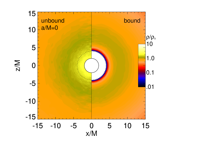
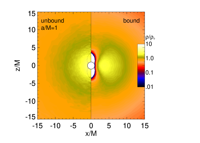
Figure 8.— Spatial density of test particles in the $x-z$ plane, for both bound and unbound populations, for $a/M=0$ and $a/M=1$. For each case, we show the unbound distribution on the left side and the bound distribution on the right side of the plot, and all distribution functions are normalized to the mean density at $r=10M$. The horizon is plotted as a solid curve and the radius of the marginally bound orbits is shown as a dotted curve. The spin axis of the black hole is in the $+z$ direction.

In Figure 8 we show the 2D density profile in the $x-z$ plane for both bound and unbound populations, for $a/M=0$ and $a/M=1$. The horizon in Boyer-Lindquist coordinates is plotted as a solid black line. For comparison purposes, the density scale is normalized to the mean value at $r=10M$. In reality, the density of the bound particles could be orders of magnitude greater at these radii (Gondolo & Silk, 1999). The most obvious difference here is the depletion of bound orbits inside of the ISCO, which lies at $r=6M$ for non-spinning black holes. For spinning black holes, the radius of the ISCO is a function of the particle’s inclination angle, ranging from $r=1M$ for prograde orbits in the equatorial plane, to $r=5.2M$ for polar orbits, and $r=9M$ for retrograde equatorial orbits.

Inside of the ISCO, there is also the “marginally bound” radius, where particles with unity specific energy can exist on unstable circular orbits. This radius is also a function of inclination angle, and is plotted in Figure 8 as dotted curve. Inside of this orbit, no bound particles will be found (for improved visibility, we have left this region white, not black, as would be required by a strict adherence to the color scale). One interesting feature of Figure 8 is that the density of the unbound population around spinning black holes doesn’t show any obvious $\theta$-dependence. It appears that the enhanced density due to long-lived prograde orbits is almost exactly countered by the lack of retrograde orbits at the same latitude.

Figure 9.— Momentum distribution of bound particles observed by a ZAMO in the equatorial plane at radius $r=100M$. Unlike the unbound distribution in Figure 4, the energy distribution is much broader here, yet with a smaller mean momentum (panel a). In panels (b-d) we show the distribution of the individual momentum components.

In Figure 9 we show the phase space distribution for each of the momentum components, as measured by a ZAMO in the equatorial plane at large radius ($r=100M$). Compared to the equivalent plot for the unbound distribution (Fig. 4), we see a number of significant differences. First, the fact that these particles are bound requires that $E<1$, and the imposed virial energy distribution results in mean velocities that are smaller than those of the unbound population by a factor of $\sim\sqrt{2}$. Second, because we require stable, long-lived orbits, there is a larger depletion around $p^{\tilde{\theta}}=0$ and $p^{\tilde{\phi}}=0$, as these trajectories are all captured by the black hole and thus do not contribute at all to the distribution function. Similarly, we see a larger asymmetry due to the preferential capture of retrograde orbits with $p^{\tilde{\phi}}<0$.

Figure 10.— Momentum distribution of bound particles observed by a ZAMO in the equatorial plane at radius $r=2M$. Compared to Figure 5, here we actually see a more symmetric, thermal distribution making up a thick torus of stable, roughly circular orbits near the equatorial plane.

In Figure 10 we plot the same momentum distribution functions, now at $r=2M$. Here the contrast with the unbound population (Fig. 5) is even greater. The only stable orbits at this radius are prograde, nearly circular, nearly equatorial orbits. This results in a relatively narrow distribution clustered around $u^{\tilde{\mu}}=[\sqrt{2},0,0,1]$ in the ZAMO frame. This narrower range in allowed velocities will have a profound impact on the shape of the annihilation spectrum, as we will see in the following section.

3. ANNIHILATION PRODUCTS

Once we have populated the distribution function, we can calculate the annihilation rate given a simple particle-physics model for the dark matter cross section. Again, it is simplest to work in the local tetrad frame. Including special relativistic corrections (Weaver, 1976), the local reaction rate is given by the following:

$$R(\mathbf{x})=\int d^{3}\mathbf{p}_{1}\int d^{3}\mathbf{p}_{2}\,f(\mathbf{x},\mathbf{p}_{1})\,f(\mathbf{x},\mathbf{p}_{2})\,\frac{\gamma_{\rm rel}}{\gamma_{1}\gamma_{2}}\,\sigma_{\chi}(\gamma_{\rm rel})\,v_{\rm rel}\,,$$ (12)

where $\gamma_{1}$ and $\gamma_{2}$ are the Lorentz factors of two particles as measured in the tetrad frame, $v_{\rm rel}$ is their relative velocity, and $\sigma_{\chi}$ is the annihilation cross section (potentially a function of the relative velocity). $R(\mathbf{x})$ has units of [events per unit proper volume per unit proper time], so we multiply by $d\tau/dt$ to get the rate observed by a distant observer.

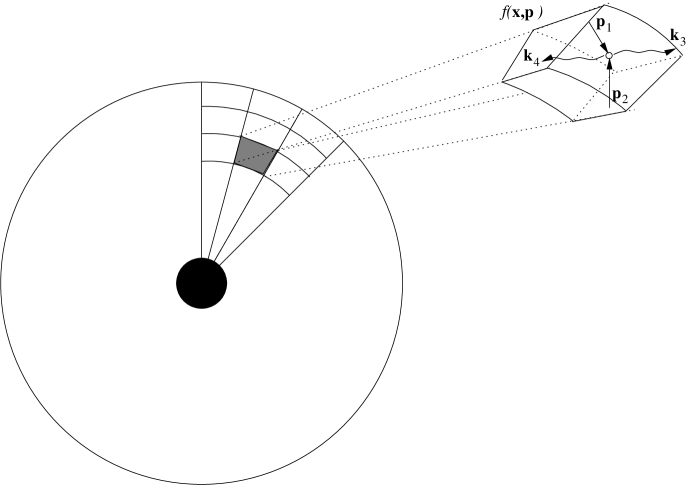
Figure 11.— For a given phase-space distribution $f(\mathbf{x},\mathbf{p})$, the annihilation rate is calculated in each discrete volume element around the black hole. Every annihilation event samples the distribution function to get the momenta for the two dark matter particles $\mathbf{p}_{1}$ and $\mathbf{p}_{2}$ and produces two photons $\mathbf{k}_{3}$ and $\mathbf{k}_{4}$ with isotropic distribution in the center-of-mass frame. The product photons then propagate along geodesics until they reach a distant observer or get captured by the black hole.

The distribution function $f(\mathbf{x},\mathbf{p})$ is calculated numerically using the methods of Section 2. As discussed there, the numerical representation of $f$ can have upwards of $10^{8}$ elements, so the direct integration of equation (12) is generally not computationally feasible. Instead, we use a Monte Carlo sampling algorithm to pick random momenta for each particle with an appropriate weight based on the magnitude of $f$ and the size of the discrete phase space volume.

The spatial integration, however, is carried out directly, looping over coordinates $r$ and $\theta$. This is shown schematically in Figure 11. For each volume element, a large number (typically $\sim 10^{6}$) of pairs of particles are sampled, and for each pair, a center-of-mass tetrad is created. The total energy in the center-of-mass frame is given by

$$E_{\rm com}=m_{\chi}\sqrt{2(1+\mathbf{u}_{1}\cdot\mathbf{u}_{2})}\,,$$ (13)

where $m_{\chi}$ is the rest mass of the DM particle, and $\mathbf{u}=\mathbf{p}/m_{\chi}$ is the particle 4-velocity.

The 4-velocity of the center-of-mass frame is then given by

$$\mathbf{u}_{\rm com}=(\mathbf{u}_{1}+\mathbf{u}_{2})/E_{\rm com}\,.$$ (14)

The center-of-mass tetrad is constructed with $\mathbf{e}_{(\tilde{t})}=\mathbf{u}_{\rm com}$. The spatial basis vectors are totally arbitrary, as they are only needed to launch photons with an isotropic distribution in the center-of-mass frame. Two photons, labeled $\mathbf{k}_{3}$ and $\mathbf{k}_{4}$ in Figure 11, are launched in opposite directions, each with energy $E_{\rm com}/2$ in the center-of-mass frame. We then transform back to a coordinate basis for the geodesic integration of the photon trajectories to a distant observer.

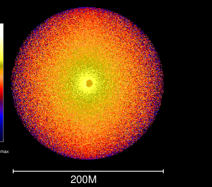
Figure 12.— Simulated image and spectrum of the annihilation signal from unbound dark matter out to a radius $r=100M$ around a Kerr black hole. The observer is located in the equatorial plane. While the brightness peaks towards the black hole, the total flux is dominated by annihilations at large radii. The central shadow is clearly seen, blocking emission coming from the far side of the black hole. The photon energy $E$ is scaled to the dark matter rest mass $m_{\chi}$.

As in Schnittman & Krolik (2013), for the photons that reach infinity, Pandurata can generate an image and spectrum of the emission region. An example in shown in Figure 12 for the annihilation signal from the unbound population around an extremal black hole, limiting the emission signal to the region $r<100M$. While the flux clearly increases towards the center of the image, because the density and velocity profiles are relatively shallow (see Fig. 2 above), the net flux is actually dominated by emission from large radii. These annihilation events are not very relativistic, so produce a strong, narrow peak in the observed spectrum, centered at the DM rest mass energy.

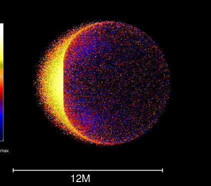
Figure 13.— Simulated image and of the annihilation signal around an extremal Kerr black hole, now considering only annihilations with $E_{\rm com}>3m_{\chi}$. The observer is located in the equatorial plane with the spin axis pointing up. While the image appears off-centered, it is actually aligned with the coordinate origin. The photon energy $E$ is scaled to the dark matter rest mass $m_{\chi}$.

The annihilation events occurring closer to the horizon sample a much more energetic population of particles. Restricting ourselves to only those events where the center-of-mass energy is greater than $1.5\times$ the combined rest mass of the annihilating particles, we can zoom in to the center of Figure 12. The result is shown in Figure 13, now focusing on the inner region within $r<6M$. At these small radii, the effects of black hole spin become much more evident. One such effect is the characteristic shape of the Kerr shadow, defined by the impact parameter of critical photon orbits (Chandrasekhar, 1983). The observed flux is clearly asymmetric, as the prograde photons originating from the left side of the image have a much greater chance of escaping the ergosphere and reaching a distant observer.

There is another interesting feature of Figure 13 that we believe is novel to this work. Namely, the purple lobes emerging from the “mid-latitude” regions near the center of the image. These are regions of greater photon flux, albeit very highly redshifted. Recall, this image is created by considering only annihilations with moderately high center-of-mass energy. Near the equatorial plane, extreme frame dragging ensures that the velocity dispersion is highly anisotropic, with most of the DM particles and their annihilation photons getting swept along on prograde, equatorial orbits. Above and below the plane, the DM distribution is more isotropic, leading to a more isotropic distribution of outgoing photons. Yet if one goes two far off the midplane, it becomes more difficult for the photons to escape. At the mid-latitudes, there is just enough frame dragging for photons to escape, yet not so much that they get deflected away from the observer.

The spectrum corresponding to this image is also plotted in Figure 13. Not surprisingly, the red and blue wings of the annihilation line shown in Figure 12 come from the most relativistic events. As pointed out by Piran & Shaham (1977), even reactions with very high center-of-mass energies will typically lead to photons with low energies as measured at infinity, thus explaining the red tail of the annihilation spectrum. The high-energy tail above $E=2m_{\chi}$ is due exclusively to Penrose-process reactions where one of the annihilation photons has negative energy and gets captured by the black hole (Penrose, 1969; Piran et al., 1975).

Earlier analytic work predicted that the maximum energy attainable from the collisional Penrose process was $2.6m_{\chi}$ for particles falling from rest at infinity (Harada et al., 2012; Bejger et al., 2012). Because our calculation is fully numerical, it was able to reveal previously unknown trajectories leading to very high efficiencies with $E>10m_{\chi}$, as seen in Figure 13. Closer inspection revealed that these high-energy photons are created when an infalling retrograde particle collides with a outgoing prograde particle that has just enough angular momentum to reflect off the centrifugal barrier, providing the necessary energy and momentum for the annihilation photon to escape the black hole (Schnittman, 2014; Berti et al., 2014).

Figure 14.— Observed annihilation spectrum for the unbound DM population, as a function of observer inclination angle, considering only annihilations with $E_{\rm com}>3m_{\chi}$. The black hole spin is $a/M=1$.

Due to the strong forward-beaming effects within the ergosphere, the escaping photon flux is highly anisotropic, with the peak flux and highest-energy photons emitted in the equatorial plane. Figure 14 shows the predicted annihilation spectra for observers at different inclination angles for the same DM profile as shown in Figure 13. Again, we restrict ourselves to the highest-energy reactions with $E_{\rm com}>3m_{\chi}$.

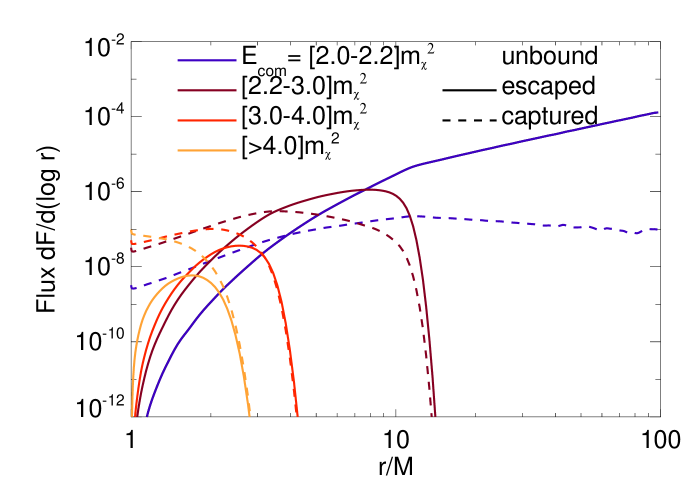
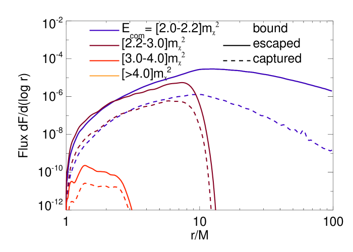
Figure 15.— Flux reaching infinity (solid curves) and getting captured by the black hole (dashed curves), as a function of the center-of-mass energy and radius of annihilation, for both bound and unbound populations. The black hole spin is maximal. Note that the scale on the y-axis is arbitrary, and depends strongly on the annihilation cross sections and peak density. The radial flux profile, on the other hand, is a robust result for these populations.

It is also instructive to plot the annihilation flux as a function of the emission radius. In Figure 15 we show both the observed flux (solid curves) and the flux that gets captured by the black hole (dashed curves) as a function of radius, integrated over all observing angles. The emission is further subdivided by the center-of-mass energy of the annihilating particles. Of course, the photons emitted closer to the black hole have a greater chance of getting captured. For the unbound population, the total escape fraction ranges from $f_{\rm esc}=93\%$ at $r=10M$ down to $f_{\rm esc}(2M)=14\%$, and $f_{\rm esc}(1.1M)=0.25\%$. At small radius, these numbers are somewhat smaller than those calculated by Bañados et al. (2011), who only considered critical trajectories in the equatorial plane, where the escape probability is greatest. Yet at large radius, our distribution includes particles with typically greater impact parameters, and thus greater chance for escape.

Another interesting feature of the curves in Figure 15 is the very sharp cutoff above a critical radius for each energy bin. This is a natural consequence of conservation of energy. Because all unbound particles come in from rest at infinity with $E=m_{\chi}$, the available kinetic energy in the center-of-mass frame is simply the gravitational potential energy $Mm_{\chi}/r$ at that radius. For example, to reach a center-of-mass energy of $10\%$ above the rest mass energy, the particles must fall within $r\approx 10M$. Also note that inside $r\approx 4M$, most of the photons are captured, while outside of this radius, most escape. This is in close agreement with what we found for plunging orbits inside of the ISCO of a Schwarzschild accretion flow in Schnittman et al. (2013).

On the other hand, for the bound population of DM particles (Fig. 15b), which by definition are not plunging, we find that the photon escape fraction is more than $90\%$ at all radii, greatly increasing the relativistic effects observable from infinity. This is consistent with the classic calculation by Thorne (1974) which found that for thin accretion disks limited to circular, planar orbits outside the ISCO, the fraction of emission ultimately captured by the black hole was never more than a few percent, even for maximally spinning black holes where the majority of the flux emerges from extremely close to the horizon.

As we showed in Schnittman (2014), the peak energy attainable from particles falling in from infinity is a strong function of the black hole spin. Now, considering the full phase-space distribution function of the particles, we can see how the shape of the spectrum depends on spin. In Figure 16 we plot the flux seen by an equatorial observer, again limited to the high-energy annihilations with $E_{\rm com}>3m_{\chi}$. For even marginally sub-extremal spins, the peak photon energy falls precipitously. As the spin decreases further, the number of collisions with $E_{\rm com}>3m_{\chi}$ also decreases, thereby reducing the total flux observed. Lastly, the decreasing spin also increases the critical impact parameter for capturing prograde photons, making it harder for the annihilation flux to escape to infinity.

Figure 16.— Observed spectrum as a function of black hole spin, for an observer at inclination $i=90^{\circ}$, considering only annihilations with $E_{\rm com}>3m_{\chi}$.

Recall from Section 2.3 above that the density of the unbound distribution scales like $n\sim r^{-1/2}$. From the rate calculation in equation (12) we see that the annihilation rate [events/s/cm³] scales like $R(r)\sim r^{-3/2}$. Including the volume factor $dV=4\pi r^{2}dr$ we can write the differential annihilation rate as $dR/dr\sim r^{1/2}$. In other words, the unbound contribution to the annihilation signal diverges at large radius. In practice, the outer boundary can be set as the black hole’s influence radius, typically $10^{6-7}r_{g}$. This means that the observed signal will essentially be a delta function in energy, with only small perturbations from the relativistic contributions at small $r$, and thus measuring spin from annihilation lines would be a very challenging prospect indeed.

Two possible effects provide a way around this problem, each with its own additional uncertainties. One possibility is that the annihilation cross section is a strong function of energy, increasing sharply above some threshold energy. This is admittedly rather speculative, and in conflict with leading DM models of self-annihilation (Bertone et al., 2005). On the other hand, we do not even know what the dark matter particle is, or if there are many DM species making up a rich “dark sector,” with all the beauty and complexity of the standard model particles (Zurek, 2014). One could easily imagine a DM analog of pion production via the collision of high-energy protons, in which case the only reactions could occur immediately surrounding a black hole, the ultimate gravitational particle accelerator. In this case, by construction the annihilation rate is dominated the region immediately surrounding the black hole.

Another possibility is that the DM density is dominated by a population of bound particles. As described above in section 2.4, this population arises through the adiabatic growth of the black hole through accretion, capturing marginally unbound particles while also making the bound particles ever more tightly bound Gondolo & Silk (1999); Sadeghian et al. (2013). This process will generally lead to a much steeper density profile, such as the $n\sim r^{-2}$ distribution we use here. In this case, the differential reaction rate scales like $dR/dr\sim r^{-5/2}$ so the annihilation spectrum is now dominated by the particles at smallest radii. In both cases—energy-dependent cross sections and a large bound population—the relativistic effects described in Section 2.3 (expanded proper volume and time dilation) push the most important interaction region to even smaller radii, and thus the annihilation spectra are even more sensitive to the black hole spin.

Figure 17.— Comparison of annihilation spectra from bound and unbound populations, including all emission out to $r=1000M$. The peak of the unbound signal will actually be even narrower, as it is dominated by annihilations at large radii with small relative velocities.

In Figure 17 we show the annihilation spectra for both the bound and unbound populations for a variety of spins, now including emission out to $r=1000M$. The relative amplitudes are somewhat arbitrary, because we don’t know what the relative densities of the two populations might be (see discussion below in Sec. 4), but it is almost certain that the bound population should dominate, possibly even by many orders of magnitude (Gondolo & Silk, 1999). At the same time, the unbound signal will be even narrower and have a greater amplitude peak than shown here, as it is dominated by low-velocity particles at large radius. So while their overall amplitudes are uncertain, the detailed shapes of the spectra away from the central peak are relatively robust, depending only on the properties of geodesic orbits near the black hole.

In this broad part of the spectrum, the bound and unbound signals show very different behavior. For non-spinning black holes, no particle can remain on a bound orbit inside of $r=4M$ (see Fig. 8), so there are no annihilation photons coming from just outside the horizon, and these are the photons that produce the most strongly redshifted tail of the spectrum. As the spin increases and the ISCO moves to smaller and smaller radii, the line becomes steadily broader. On the other hand, the unbound particles are found all the way down to the horizon, where they can annihilate to highly redshifted photons regardless of the black hole spin.

Comparing Figures 5 and 10, we see that the unbound particles probe a much greater volume of momentum space at small radii. This in turn leads to a greater chance of producing the extreme Penrose particles that characterize the blue tail of the spectrum. Because all the bound particles are essentially on the same prograde, equatorial orbits, it is much more difficult to achieve annihilations with large center-of-mass energies, so the high-energy cutoff in the spectrum is much closer to the classical result for a single particle decaying into two photons in the ergosphere (Wald, 1974). In short, for bound particles the red tail of the spectrum is a better probe of black hole spin, while for the unbound population, the blue tail is the more sensitive feature. But in both cases, higher spin leads to a broader annihilation line.

4. OBSERVABILITY

In addition to the dependence on the dark matter density profile, the amplitude of the annihilation spectrum will also depend on the unknown dark matter mass and annihilation cross section. At this point, it is only possible to use existing observations to set upper limits on these unknown parameters. One major obstacle that has plagued nearly all observational efforts to detect dark matter annihilation is the existence of more conventional astrophysical objects such as active galactic nuclei (AGN), pulsars, and supernova remnants, all of which are powerful sources of high energy gamma rays. One solution to this problem is to focus on nearby dwarf galaxies, which are thought to have a high DM fraction and are not typically contaminated by AGN activity or significant star formation (Ackermann et al., 2011) (note, however, the recent work by Gonzalez-Morales et al. (2014), which focuses on the contribution of black holes in dwarf galaxies).

Yet for our purposes, it turns out that the strongest upper limits actually come from the most massive galaxies with the most massive central black holes. Massive elliptical galaxies have the added advantage of being relatively quiescent both in nuclear activity and star formation [e.g., Schawinski et al. (2007)]. As mentioned above, the annihilation signal from the unbound population will be dominated by flux at large radius. It is difficult enough to spatially resolve even nearby black holes’ influence radii with HST, much less gamma-ray telescopes, so any potential annihilation signal will tell us little about the black hole itself.

Prospects for detection of an unambiguous black hole signature improve if we consider annihilation models that include an energy dependence to the dark matter cross section. For example, p-wave annihilation mechanisms will have cross sections proportional to the relative velocity between the two annihilating particles [see Chen & Zhou (2013); Ferrer & Hunter (2013) and references therein]. Unfortunately, from equation (11) we see that this would only lead to an additional factor of $r^{-1/2}$ in the integrand of equation (12), which would still be dominated by the contributions from large $r$.

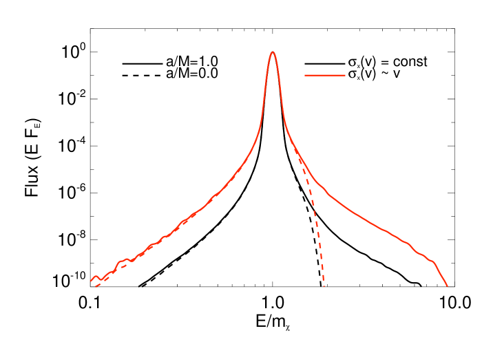
Figure 18.— Comparison of annihilation spectra from unbound populations, for two simple models of the dark matter cross section. All spectra are normalized to their peak intensity. For this comparison, all emission within $r=10^{4}M$ is included.

This effect is shown in Figure 18, which plots the predicted spectra for two annihilation models: $\sigma_{\chi}(v)=\mbox{const}$ (black curves) and $\sigma_{\chi}(v)\propto v$ (red curves). The black hole spins considered are $a/M=0$ (dashed curves) and $a/M=1$ (solid curves), and in all cases only the unbound population is included. Integrating out to $r=10^{4}M$, we see only a slight difference in the shape of the spectrum, with the $\sigma_{\chi}(v)\propto v$ model leading to a slightly broader peak (all curves are normalized to give a peak amplitude of unity).

Another possible annihilation model is based on a resonant reaction at some energy above the DM rest mass, as suggested in Baushev (2009). If the cross section increases sharply around a given center-of-mass energy, this would have the effect of focusing in on a relatively narrow volume of physical space around the black hole, as in Figure 15.

Alternatively, the cross section could abruptly increase above a certain threshold energy, if new particles in the dark sector become energetically allowed, analogous to pion production via proton scattering. In either the resonant or threshold models for the annihilation cross section, one might imagine a pair of heavier, intermediate dark particles getting created and then annihilating to two photons as in the direct annihilation model. If, for example, the mass of these intermediate particles is $1.5m_{\chi}$, then the observed spectrum would look like those plotted in Figures 13 and 16. With a significant increase in the cross section above such an energy threshold, these relativistically-broadened spectra could in fact dominate over the narrow line component produced by the rest of the galaxy.

A less exotic option would be the simple density enhancement due to the bound population. If this is sufficiently large, it would easily dominate over the rest of the galaxy and also produce a characteristically broadened line sensitive to both black hole spin magnitude and orientation relative to the observer. Somewhat ironically, one of the things that could ultimately limit the strength of the annihilation signal from bound dark matter is annihilation itself. If the adiabatic black hole growth occurred at high redshift, then in the subsequent $\sim 10^{10}$ years, the bound population will get depleted via self-annihilation at an accelerated pace due to its high density (Gondolo & Silk, 1999; Gonzalez-Morales et al., 2014).

On the other hand, if the black hole grows through mergers, or experiences even a single merger since the last extended accretion episode, it is quite likely that the bound dark matter population could get completely disrupted. The details of such an event are beyond the scope of this paper, but could be modeled by following test particles bound to each black hole through the merger, via post-Newtonian calculations (Schnittman, 2010) or numerical relativity (van Meter et al., 2010).

The observational challenge is readily apparent: the black holes with the largest bound populations will tend to be in gas-rich galaxies with a lot of accretion and high-energy nuclear activity that could overwhelm the DM annihilation signal. The more massive black holes, residing in gas-poor quiescent galaxies, are also more likely to have lost their cloud of bound dark matter through a history of mergers. Even in the event that a gas-rich spiral galaxy hosts a quiescent nucleus, the black holes in those galaxies tend to have lower masses (Kormendy & Ho, 2013).

While the relation between black hole mass and dark matter density is quite complicated for the bound population, it is relatively straightforward to calculate for the unbound population, which we can take as a lower bound on the DM density. Recall the influence radius $r_{\rm infl}$ is the distance within which the gravitational potential is dominated by the black hole, as opposed to the nuclear star cluster or dark matter halo. From equation (2) we see that the influence volume scales like $r_{\rm infl}^{3}\sim M^{3/2}$, while the total mass enclosed is—by definition—of the order of $M$. If the dark matter and baryonic matter have similar profiles (by no means a certainty!), then more massive black holes should have lower surrounding DM density, with $n_{\rm infl}\sim M^{-1/2}$.

Because the unbound DM density falls off more rapidly outside the central core, the annihilation flux $F_{\rm unbound}$ will be dominated by the contribution from around $r_{\rm infl}$, so we can estimate

$$F_{\rm unbound}\approx\frac{1}{D^{2}}n_{\rm infl}^{2}\sigma_{\chi}v_{\rm infl}r_{\rm infl}^{3}\sim M^{3/4}\,D^{-2}\,,$$ (15)

with $D$ the distance to the black hole and the mean velocity at the influence radius $v_{\rm infl}=\sigma_{0}$.

If we consider a threshold energy annihilation model where all the flux comes from inside a critical radius $r_{\rm crit}\sim\mbox{few}\times r_{g}$, then the density scales like $n_{\rm crit}\sim n_{\rm infl}(r_{\rm infl}/r_{\rm crit})^{1/2}\sim M^{-3/4}$ while the relative velocity scales like $v_{\rm crit}\sim\sigma_{0}(r_{\rm infl}/r_{\rm crit})^{1/2}\sim M^{0}$. The net flux then scales like

$$F_{\rm unbound}\approx\frac{1}{D^{2}}n_{\rm crit}^{2}\sigma_{\chi}v_{\rm crit}r_{\rm crit}^{3}\sim M^{3/2}\,D^{-2}\,.$$ (16)

In both cases, it appears that the brightest sources will be the closest, as opposed to the most massive.

Now consider the case where the annihilation signal is dominated by the bound contribution, the bound density is in turn limited by a self-annihilation ceiling as in Gondolo & Silk (1999), and there is a threshold energy above which the cross section greatly increases. In this case, the flux is simply proportional to the total volume within the critical radius, so $F_{\rm bound}\sim M^{3}\,D^{-2}$. With this scaling, the greatest flux will actually come from more distant, more massive black holes. For example, NGC 1277, with a mass of $1.7\times 10^{10}M_{\odot}$ and at a distance of 20 Mpc (van den Bosch et al., 2012), could give an observed flux over a thousand times greater than our own Sgr A^∗!

Recent works by Fields et al. (2014) and Gonzalez-Morales et al. (2014) have argued that current Fermi limits of gamma-ray flux from Sgr A^∗ and nearby dwarf galaxies with massive black holes already place the strongest limits on annihilation from DM density spikes. Based on the arguments above, we believe that even stronger limits should come from more distant, massive galaxies. The other important advance presented in the present work is that, for either the energy-dependent cross sections, or the steep density spikes, the annihilation signal will be dominated by the region closest to the black hole, and thus a fully numerical, relativistic rate calculation is absolutely essential.

Lastly, we should mention that gamma-rays, while the primary observable feature explored in this work, are not the only promising annihilation product. High-energy neutrinos could also be produced in some annihilation channels, particularly those with energy-dependent cross sections like p-wave annihilation (Bertone et al., 2005). While neutrinos obviously present many new detection challenges, the successful commissioning of new astronomical observatories like IceCube make this approach an exciting prospect (Aartsen et al., 2013). Furthermore, the non-DM backgrounds may contribute significantly less confusion in the neutrino sky.

5. DISCUSSION

As apparent in the previous section, there are still far too many unknown model parameters to allow for quantitative predictions of the annihilation flux from dark matter around black holes. Sadeghian et al. (2013) put it best: “There are uncertainties in all aspects of these models. However one thing is certain: if the central black hole Sgr A^∗ is a rotating Kerr black hole and if general relativity is correct, its external geometry is precisely known. It therefore makes sense to make use of this certainty as much as possible.” We have attempted to follow their advice to the best of our ability.

Thus, in order of decreasing confidence, the results in this paper can be summarized by the following:

• For a given DM density $n_{\rm infl}$ and velocity dispersion $\sigma_{0}$ at the black hole’s influence radius, the fully relativistic, 5-dimensional phase-space distribution has been calculated exactly for any black hole spin parameter, covering the region from $r_{\rm infl}$ all the way down to the horizon.

• Given this distribution function and a model for dark matter annihilation, the observed gamma-ray spectrum can be calculated by following photons from their creation until they are either captured by the black hole or reach the observer. Two important relativistic effects serve to increase the annihilation rate as compared to a purely Newtonian treatment: time dilation near the black hole effectively raises the density of the unbound population in a steady-state distribution being fed from infinity; and transforming from coordinate to proper distances greatly increases the interaction volume in the region immediately around the black hole (see Fig. 3).

• Our numerical approach has unveiled previously overlooked orbits that can produce annihilation photons with extreme energies, far exceeding previous estimates for the maximum efficiency of the collisional Penrose process (Schnittman, 2014). The peak energy attainable for escaping photons is a strong function of the black hole spin.

• The population of bound dark matter has also been calculated numerically, although this depends on two additional physical assumptions: a local isothermal velocity distribution with a virial-like temperature; and an overall radial power-law for the density, as found in Gondolo & Silk (1999) and Sadeghian et al. (2013). Including only the long-lived stable orbits, we found that the density peaks in the equatorial plane somewhat outside of the ISCO, forming a thick, co-rotating torus around the black hole spin axis. Because the bound population is not plunging towards the horizon, the emerging flux has a much greater chance of escaping the black hole.

• The annihilation spectra from both the bound and unbound populations are sensitive to the spin parameter, but in opposite ways: the unbound spectrum varies mostly in the high-energy cutoff, with higher spins allowing higher-energy annihilation products; the bound population moves closer and closer to the horizon with increasing spin, giving a stronger red-shifted tail to the annihilation spectrum. Both bound and unbound spectra become more sensitive to observer inclination with increasing spin, as the spherical symmetry of the system is broken.

• For dark matter particle physics models with an energy-dependent cross section (particularly one that increases with center-of-mass energy), the annihilation spectrum will be a more sensitive probe of the black hole properties. For DM models incorporating a rich population of dark sector species, black holes may be the most promising way to accelerate these particles and observe their interactions.

• The shape of the annihilation spectra is relatively robust, but the normalization is highly dependent on uncertain parameters such as the dark matter density profile and cross section. If the unbound density profile follows the baryonic matter, with the shallow slopes seen in core galaxies, the observed flux should be a relatively weak function of black hole mass. If, on the other hand, the annihilation signal is produced by the most relativistic population within $r_{\rm crit}\sim\mbox{few}\times r_{g}$, then the signal could scale like $M^{3}$ and thus be dominated by the most massive black holes in the local Universe.

While this paper has treated the bound and unbound particles separately, future work will also consider the self-interaction between these two populations (Shapiro & Paschalidis, 2014; Fields et al., 2014), which may lead to a single, self-consistent steady-state distribution with density slope between $-1/2$ and $-2$. Future work will also focus on developing a robust framework in which we can use existing and future gamma-ray observations to constrain various parameters of the particle physics (e.g., $m_{\chi}$, $\sigma_{\chi}(E)$, and the annihilation mechanism, i.e., line vs continuum) and astrophysical models ($n_{\rm infl}$, the bound distribution normalization and slope, and the black hole mass, spin, and inclination). While initial work will focus on setting upper limits on reaction rates by looking at quiescent galaxies, our ultimate ambition is nothing short of an unambiguous detection of dark matter annihilation around supermassive black holes.

References

- Aartsen et al. (2013) Aartsen, M. G., Abbasi, R., Abdou, Y., et al. 2013, Physical Review Letters, 110, 131302
- Ackermann et al. (2011) Ackermann, M., Ajello, M., Albert, A., et al. 2011, Physical Review Letters, 107, 241302
- Bañados et al. (2011) Bañados, M., Hassanain, B., Silk, J., & West, S. M. 2011, Phys. Rev. D, 83, 023004
- Bañados et al. (2009) Bañados, M., Silk, J., & West, S. M. 2009, Physical Review Letters, 103, 111102
- Bahcall & Wolf (1976) Bahcall, J. N., & Wolf, R. A. 1976, ApJ, 209, 214
- Bardeen et al. (1972) Bardeen, J. M., Press, W. H., & Teukolsky, S. A. 1972, ApJ, 178, 347
- Baushev (2009) Baushev, A. 2009, International Journal of Modern Physics D, 18, 1195
- Bejger et al. (2012) Bejger, M., Piran, T., Abramowicz, M., & Håkanson, F. 2012, Physical Review Letters, 109, 121101
- Berti et al. (2014) Berti, E., Brito, R., & Cardoso, V. 2014, ArXiv e-prints, arXiv:1410.8534
- Bertone et al. (2005) Bertone, G., Hooper, D., & Silk, J. 2005, Phys. Rep., 405, 279
- Boyer & Lindquist (1967) Boyer, R. H., & Lindquist, R. W. 1967, Journal of Mathematical Physics, 8, 265
- Chandrasekhar (1983) Chandrasekhar, S. 1983, The mathematical theory of black holes
- Chen & Zhou (2013) Chen, J., & Zhou, Y.-F. 2013, Journal of Cosmology and Astroparticle Physics, 4, 17
- Ferrarese & Merritt (2000) Ferrarese, L., & Merritt, D. 2000, ApJ, 539, L9
- Ferrer & Hunter (2013) Ferrer, F., & Hunter, D. R. 2013, Journal of Cosmology and Astroparticle Physics, 9, 5
- Fields et al. (2014) Fields, B. D., Shapiro, S. L., & Shelton, J. 2014, Physical Review Letters, 113, 151302
- Gnedin & Primack (2004) Gnedin, O. Y., & Primack, J. R. 2004, Physical Review Letters, 93, 061302
- Gondolo & Silk (1999) Gondolo, P., & Silk, J. 1999, Physical Review Letters, 83, 1719
- Gonzalez-Morales et al. (2014) Gonzalez-Morales, A. X., Profumo, S., & Queiroz, F. S. 2014, Phys. Rev. D, 90, 103508
- Harada et al. (2012) Harada, T., Nemoto, H., & Miyamoto, U. 2012, Phys. Rev. D, 86, 024027
- Jacobson & Sotiriou (2010) Jacobson, T., & Sotiriou, T. P. 2010, Physical Review Letters, 104, 021101
- Jüttner (1911) Jüttner, F. 1911, Annalen der Physik, 339, 856
- Kormendy & Ho (2013) Kormendy, J., & Ho, L. C. 2013, ARA&A, 51, 511
- McWilliams (2013) McWilliams, S. T. 2013, Physical Review Letters, 110, 011102
- Penrose (1969) Penrose, R. 1969, Nuovo Cimento Rivista Serie, 1, 252
- Piran & Shaham (1977) Piran, T., & Shaham, J. 1977, Phys. Rev. D, 16, 1615
- Piran et al. (1975) Piran, T., Shaham, J., & Katz, J. 1975, ApJ, 196, L107
- Sadeghian et al. (2013) Sadeghian, L., Ferrer, F., & Will, C. M. 2013, Phys. Rev. D, 88, 063522
- Schawinski et al. (2007) Schawinski, K., Thomas, D., Sarzi, M., et al. 2007, MNRAS, 382, 1415
- Schnittman (2010) Schnittman, J. D. 2010, ApJ, 724, 39
- Schnittman (2014) —. 2014, Physical Review Letters, 113, 261102
- Schnittman & Krolik (2013) Schnittman, J. D., & Krolik, J. H. 2013, ApJ, 777, 11
- Schnittman et al. (2013) Schnittman, J. D., Krolik, J. H., & Noble, S. C. 2013, ApJ, 769, 156
- Shapiro & Paschalidis (2014) Shapiro, S. L., & Paschalidis, V. 2014, Phys. Rev. D, 89, 023506
- Thorne (1974) Thorne, K. S. 1974, ApJ, 191, 507
- van den Bosch et al. (2012) van den Bosch, R. C. E., Gebhardt, K., Gültekin, K., et al. 2012, Nature, 491, 729
- van Meter et al. (2010) van Meter, J. R., Wise, J. H., Miller, M. C., et al. 2010, ApJ, 711, L89
- Wald (1974) Wald, R. M. 1974, ApJ, 191, 231
- Weaver (1976) Weaver, T. A. 1976, Phys. Rev. A, 13, 1563
- Williams (1995) Williams, R. K. 1995, Phys. Rev. D, 51, 5387
- Williams (2004) —. 2004, ApJ, 611, 952
- Zeldovich & Novikov (1971) Zeldovich, Y. B., & Novikov, I. D. 1971, Relativistic astrophysics. Vol.1: Stars and relativity
- Zurek (2014) Zurek, K. M. 2014, Phys. Rep., 537, 91