Are the gyro-ages of field stars underestimated?

By using the current photometric rotational data on eight galactic open clusters, we show that the evolutionary stellar model (isochrone) ages of these clusters are tightly correlated with the period shifts applied to the $(B-V)_{0}$–$P_{\rm rot}$ ridges that optimally align these ridges to the one defined by Praesepe and the Hyades. On the other hand, when the traditional Skumanich-type multiplicative transformation is used, the ridges become far less aligned due to the age-dependent slope change introduced by the period multiplication. Therefore, we employ our simple additive gyro-age calibration on various datasets of Galactic field stars to test its applicability. We show that, in the overall sense, the gyro-ages are systematically greater than the isochrone ages. The difference could exceed several giga years, depending on the stellar parameters. Although the age overlap between the open clusters used in the calibration and the field star samples is only partial, the systematic difference indicates the limitation of the currently available gyro-age methods and suggests that the rotation of field stars slows down with a considerably lower speed than we would expect from the simple extrapolation of the stellar rotation rates in open clusters.

1 Introduction

Gyrochronology (the determination of stellar ages from their rotation periods and colors) has gained considerable popularity in recent years, largely due to the speedily accumulating observational data on open clusters. These data suggest that stars, after several ten million years of formation, settle on a fairly well-defined ridge in the color$-$rotation period ($P_{\rm rot}$) diagram. By comparing cluster data of various ages, it turned out that the height of these ridges (i.e., the rotation periods at each color) increases as the cluster is aging. This property has first been recognized by Skumanich (skumanich1972 (1972)) (see also Kraft kraft1967 (1967)) and has later been elaborated by many authors both observationally (e.g., Barnes barnes2003 (2003)) and theoretically (e.g., Kawaler kawaler1988 (1988)). Although differing in details, it is widely accepted that the slowing-down of the rotation is due to the angular momentum loss by magnetized stellar wind (as first described by Schatzman schatzman1962 (1962)), and the rotation period is scaled as the square root of the stellar age (as suggested first by Skumanich). A comprehensive description of the current status of the field of stellar rotation can be found, for example, in Bouvier (bouvier2013 (2013)).

The success of the applicability of gyrochronology depends on various factors, most importantly on the validity of the relation derived from open clusters for other stars. Based on a rather limited sample, Barnes (barnes2009 (2009)) have shown that both the chromospheric and the isochrone ages are considerably greater than the gyro-ages derived from his formulae. Similarly, Brown (brown2014 (2014)) investigated a more extended sample of transiting extrasolar planet host stars and found hints of this effect. Two very recent papers seem to further strengthen this observation. Angus et al. (angus2015 (2015)) performed a Monte Carlo Markov chain analysis by using $310$ asteroseismic targets from the archive of the Kepler satellite, a few well-studied fields stars from other earlier works, and data on two open clusters. They calibrated the formula of Barnes (barnes2003 (2003)) on this merged dataset. They found that the marginalized likelihoods of the gyro-parameters exhibit multiple maxima. The authors suggest the presence of multiple rotation-color-age populations and raise concerns for the currently applied method of gyrochronology. In a further paper, Maxted, Serenelli, & Southworth (maxted2015 (2015)) found strong evidence for the younger gyro-ages of many of the $28$ extrasolar planet host stars in their sample (largely discovered by ground-based surveys). They searched for a possible cause of the discrepancy within the framework of tidal interaction between the planet and the host, but they found no compelling evidence for a relation between the gyro-age and the computed timescale of tidal interaction.

There are also technical details, including the transformation of the color and period values to stellar ages. This is usually done by the type of formulae introduced by Barnes (barnes2003 (2003)), where, by maintaining the Skumanich-type age dependence, the color dependence of the period is represented by a multiplicative factor that entirely depends on the color. We show that this representation is suboptimal because it does not lead to the cleanest average color$-P_{\rm rot}$ ridge when, using the prescribed time-dependence, all periods are transformed to the same age. Yet another, equally important question is if the target star has already reached (and is still in) the rotationally settled state (corresponding to sequence ‘I’ in the nomenclature of Barnes barnes2003 (2003)). Open clusters are vital objects to define this state since their members are assumed to be coeval, leading to a topographically well-defined ridge structure in the color$-P_{\rm rot}$ plane. However, for individual targets we do not have any criterion to decide whether they are in the rotationally settled state, except that we assume that for their estimated ages they are. This is a general problem in the applicability of gyrochronology.

The purpose of this paper is to derive an updated relation between the color, rotation period, and age of rotationally settled stars in open clusters and employ this relation on various independent datasets to test the new formula against isochrone ages and, if possible, improve the gyro-method and extend its applicability. Except for using the isochrone ages, we stay within a strictly empirical framework throughout the paper.

2 New color-period-age formula

The ‘I’ branches of the cluster rotational data are commonly fitted by the following expression (Barnes barnes2003 (2003))

$$P=g(t)f(B-V)\hskip 5.69054pt,$$ (1)

where the age-dependent factor $g(t)$ is approximated by a power-law expression of $t^{n}$ with $n\approx 0.5$ in a broad agreement with the Skumanich-law. The color-dependent factor is also represented as a power law: $a(B-V-c)^{b}$, where $a$, $b,$ and $c$ are constant parameters determined by some properly chosen cluster; $B-V$ is assumed to be free of reddening.

In a brief test of this multiplicative age dependence, we transformed two clusters (Pleiades (M45) and NGC 6811) to the fiducial ridge line (determined by Praesepe (M44) and the Hyades – see Sect. 2.2). The multiplicative and additive period transformations are shown in the upper and lower panels of Fig. 1. The change in slope for the younger cluster M45 in the case of the multiplicative transformation is clear (see also Cargile et al. cargile2014 (2014), their Fig. 12). For NGC 6811 there is not much difference between the two types of transformation. However, we see (although the color range is rather short) that in both cases there is a slight downward trend with respect of the fiducial ridge. It might be that the steeper slope for young clusters changes toward a milder slope and eventually reverses for older clusters. Unfortunately, NGC 6811 is the only available cluster with high-quality rotational periods at $\sim 1$ Gyr, so the empirical confirmation of the evolution of slope needs to await future observations of older clusters. Because of the considerably better performance of the additive period transformation in the younger age range, in the next sections we therefore derive a new calibration of the gyro-age relation based on the additive method.

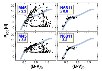
Figure 1: Multiplicative vs. additive ridge alignments. Upper panels show the result of the exact Skumanich-type period scaling with $P_{\rm rot}\rightarrow P_{\rm rot}\sqrt{t_{\rm M44}/t_{\rm cluster}}$, where $t$ stands for cluster ages. The scaling factors are displayed in the boxes. The lower panels show the same test with the additive scaling of $P_{\rm rot}\rightarrow P_{\rm rot}+c$, where $c$ is the period shift as shown in the corresponding boxes. The fiducial ridge (see Eq. (3)) is plotted as a light color continuous line.

2.1 Calibrating datasets

We chose eight recently observed clusters with reliable colors and periods. The basic properties of these clusters that are relevant for this paper are listed in Table 1. The ages span the range between $\sim 0.1$ and $\sim 1$ Gyr. Unfortunately, for older clusters (more relevant for the field stars) we do not yet have good rotation period data. For example, for one of the oldest open clusters, M67, the available rotation data are too sparse to be considered useful in the present context (e.g., Canto Martins et al. martins2011 (2011); Stassun et al. stassun2002 (2002)). For NGC 6819 (age $\sim 2.5$ Gyr, see Balona et al. 2013b ), it is hard to reconcile the color-period plot assuming that the cluster members are coeval. For NGC 6866 (age $\sim 0.65$ Gyr, see Balona et al. 2013a ), the same diagram is cleaner but still confusing (nearly constant period of $\sim 10$ days from $(B-V)_{0}\approx 0.5$ with a nearly uniform downward scatter between $\sim 2$ and $\sim 10$ days).

Although from both an observational and theoretical point of view, the use of $(B-V)_{0}$ as the color coordinate in the rotational studies is not necessary the best one, it is commonly used. Therefore, we follow this practice here as well and use the previously published $(B-V)$ colors whenever possible as given in the corresponding papers where the rotational periods were published. Four clusters (M34, M35, M45, and Blanco 1) fall into this category. For M44, we also use the $(B-V)$ colors published in our period source (i.e., in Kovács et al. kovacs2014 (2014)) but we note that the colors originate from the APASS database (via the UCAC4 catalog, see Zacharias et al. zacharias2013 (2013)). For M37 we use the colors given in the period source (Hartman et al. hartman2009 (2009)), which are based on the cluster study of Kalirai et al. (kalirai2001 (2001)), however. For NGC 6811 we cross-correlate the list of rotational variables of Meibom et al. (2011a ) with the photometric table of Janes et al. (janes2013 (2013)). This yields $58$ objects from the original $71$ objects of Meibom et al. (2011a ). For the Hyades we use the compilation of colors as given in the period source by Delorme et al. (delorme2011 (2011)). Six stars in this source do not have color values. We checked the APASS database for these objects and found that five of these have fine $B$, $V$ measurements. Before entering these values, we cross-correlated the other stars of Delorme et al. (delorme2011 (2011)) with the APASS database and found that on the average the APASS $(B-V)$ indices are $0.04$ mag bluer than the ones given in Delorme et al. (delorme2011 (2011)), that is, $(B-V)_{\rm compilation}=(B-V)_{\rm APASS}+0.04$. By applying this color shift to the APASS colors of the five variables mentioned above, we finally compiled a sample with $61$ variables for the Hyades.

Table 1: Calibrating clusters

Cluster	E(B-V)	Age [Gyr]	$N_{\rm LC}$	Source
Blanco 1	$0.02$	$0.117\pm 0.017$	33	C09, C10, C14
M45	$0.04$	$0.135\pm 0.015$	251	B14, B14, H10
M35	$0.20$	$0.180\pm 0.020$	418	K03, K03, M09
M34	$0.07$	$0.220\pm 0.030$	118	C79, M11b, M11b
M37	$0.23$	$0.550\pm 0.030$	575	H08, H08, H09
Hyades	$0.00$	$0.625\pm 0.050$	61	T80, P89, D11
M44	$0.03$	$0.665\pm 0.011$	180	T06, B14, K14
NGC6811	$0.07$	$1.000\pm 0.170$	58	J13, J13, M11a

Notes: All ages result from isochrone fits. $N_{\rm LC}=$ number of light curves; source: papers used for reddening, age and rotation periods. We assigned arbitrary age errors to M34 and M35. For these two clusters we used the published dereddened colors. For M35 Meibom, Mathieu & Stassun (meibom2009 (2009)) did not specify the reddening correction used. See text on the sources of the colors used for the clusters entered in this table.

$E(B-V)$ source: C09=Cargile, James & Platais (cargile2009 (2009)), B14=Bell et al. (bell2014 (2014)), K03=Kalirai et al. (kalirai2003 (2003)), C79=Canterna, Crawford & Perry (canterna1979 (1979)), H08=Hartman et al. (hartman2008 (2008)), T80=Taylor (taylor1980 (1980)), T06=Taylor (taylor2006 (2006)), J13=Janes et al. (janes2013 (2013))

Age source: C10=Cargile, James & Jeffries (cargile2010 (2010)) (from their Fig. 3), B14=Bell et al. (bell2014 (2014)), K03=Kalirai et al. (kalirai2003 (2003)), M11b=Meibom et al. (2011b ), H08=Hartman et al. (hartman2008 (2008)), P98=Perryman et al. (perryman1998 (1998)), J13=Janes et al. (janes2013 (2013))

Period source: C14=Cargile et al. (cargile2014 (2014)), H10=Hartman et al. (hartman2010 (2010)), M09=Meibom et al. (meibom2009 (2009)), M11b=Meibom et al. (2011b ), H09=Hartman et al. (hartman2009 (2009)), D11=Delorme et al. (delorme2011 (2011)), K14=Kovács et al. (kovacs2014 (2014)), M11a=Meibom et al. (2011a )

2.2 Fiducial color–period ridge, age scaling

As we have discussed in the introduction of this section, the strong variation in the steepness of the color-period ridges when a Skumanich-type multiplicative period transformation is used suggests that there is a need for some other type of transformation if we assume that these ridges are related through some simple, few-parameter transformation. Visual inspection of the various cluster data suggests that a simple vertical (i.e., period) shift may substantially improve the ridge alignment. Therefore, we assumed that there exists a fiducial ridge that yields a better representation of the data simply by an optimum shift of this ridge, that is, the rotation periods of the stars on the ridge of each cluster can be represented by the following formula

$$P_{\rm rot}{\rm(age,color)}=P_{\rm rot}^{\rm fiducial}{\rm(color)}-c{\rm(age)}\hskip 5.69054pt,$$ (2)

where we assumed that the additive constant is primarily a function of age. The derivation of the additive gyro-age relation requires determining the fiducial ridge and the cluster-by-cluster period shifts. In the earlier version of the paper we employed an iterative scheme of least squares with data point density as weights to derive the main fiducial ridge as the best polynomial approximation for the high-density ‘I’ branch part of the $(B-V)_{0}-P_{\rm rot}$ diagram. The derived fiducial ridge was rather close to the one spanned by Praesepe. In part due the stimulation of the referee report, we therefore decided to fix the fiducial ridge as a polynomial fit to the merged data of Praesepe and the Hyades. Some details of the fitting procedure are given in Appendix A. Here we only give the finally accepted fourth-order polynomial expression

$$P_{\rm rot}^{\rm fiducial}= - 35.51+153.07(B-V)_{0}-201.13(B-V)_{0}^{2}$$ (3)

$$\pm \phantom{3}7.71\pm\phantom{1}33.07\phantom{(B-V)_{0}}\pm\phantom{2}50.84$$

$$+ 120.60(B-V)_{0}^{3}-26.28(B-V)_{0}^{4}$$

$$\pm \phantom{1}33.35\phantom{(B-V)_{0}}\pm\phantom{2}7.91\hskip 5.69054pt.$$

This polynomial fits the periods of the two clusters with $\sigma_{\rm fit}=1.088$ days. The errors listed are $1\sigma$ formal errors.

We need to note here that the clusters used to derive this fiducial ridge exhibit fairly clean color$-P_{\rm rot}$ diagrams, including the lack of major ambiguities concerning the relation of the true rotational period to the one determined by the highest peak in the frequency spectrum. There is a generic degeneracy in this respect in all photometrically determined rotation periods. They are ambiguous toward integer multiple periods due to possible special spot positions and numbers and also for aliasing in the case of ground-based observations. We show a clear example of the period ambiguity in Fig. 2. The number of ambiguous periods changes from cluster to cluster and have some influence on the resulting period shifts. However, our experience shows that although this correction is important in principle, in practice (in part due to the relatively small number of ambiguous cases) it does not have a significant effect on the robust period shift estimation described below.

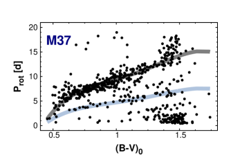
Figure 2: Example of the period adjustment based on the harmonic ambiguity of the estimated rotation periods from the frequency spectra of the light curves (Hartman et al. hartman2009 (2009)). The darker gray line shows the fiducial ridge line shifted to the cluster ‘I’ sequence. The lighter gray line was obtained by halving the periods corresponding to this cluster ridge line. The uncorrected (i.e., originally published) periods are displayed as black dots.

Several ways are possible to find the fiducial ridge line that best fits an ensemble of points that contains the cluster ridge line (sequence ‘I’) as a subset. Manual selection of outliers is one possibility, weighting with the density of the data points is another. Here we resorted to a robust fitting method that is based on a special kernel function employed in the least-squares fit. The kernel will automatically put less weight on outliers, and we do not need to decide on a case-by-case basis whether the given data point is an outlier or not.

From the several kernels available in the literature, we chose the one introduced by German & McClure (german1987 (1987)). The GM kernel is widely used in various robust fit problems, including pattern recognition (e.g., Yang et al. yang2014 (2014)). Accordingly, we minimized the following expression to find the best-fitting fiducial ridge

$$E = \sum_{i=1}^{n}G(\delta P(i))$$

$$G(\delta P(i)) = (\delta P(i))^{2}\over a+(\delta P(i))^{2}$$

$$\delta P(i) = P_{\rm rot}^{\rm fiducial}(i)-P_{\rm rot}(i)-c\hskip 5.69054pt.$$ (4)

This least-squares condition with the GM kernel is equivalent to a weighted ordinary least-squares condition with Cauchy weights. We used simple scanning to find the best-fitting period shift parameter $c$. The error of $c$ is estimated as $\sigma^{2}(c)=\sum_{i=1}^{n}w(i)(\delta P(i))^{2}/(n\sum_{i=1}^{n}w(i))$, where $w(i)=1/(a+(\delta P(i))^{2})$. The method has a single free parameter $a$ that can be tuned to be more ($a$ is small) or less ($a$ is large) sensitive to outliers. We found that $a=1$ yields a perfect performance with accurate and robust identification of the ‘I’ sequences in each cluster, with all data listed in Table 1 left in the datasets for each cluster. An example of the cluster fit is shown in Appendix A. The optimum period shifts with their errors are summarized in Table 2.

To illustrate the difference between the additive and multiplicative (Skumanich-type) period transformations on the full sample of open clusters used in this paper, in Figs. 3 and 4 we plot all data points after applying these transformations. It is clear that the additive transformation leads to a tighter pattern for the ‘I’ sequence and thereby allows a more reliable investigation of the age dependence of the rotation periods throughout the $(B-V)_{0}$ color range of $\sim(0.5-1.4)$.

Table 2: Period shifts for the calibrating clusters

Blanco 1	M45	M35	M34	M37	Hyades	M44	N6811
$3.08$	$3.48$	$3.37$	$2.53$	$1.31$	$0.05$	$0.01$	$-3.16$
$\pm 0.17$	$\pm 0.08$	$\pm 0.07$	$\pm 0.11$	$\pm 0.05$	$\pm 0.12$	$\pm 0.05$	$\pm 0.11$

Notes: The shifts (parameter $c$ in Eq. (2)) are given in days. Equations (2) and (3) can be used to predict the ridge periods for each cluster.

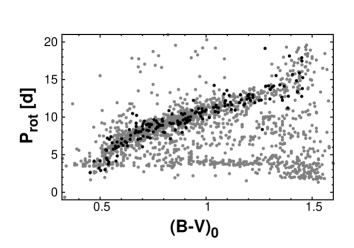
Figure 3: Merged data of the eight clusters of Table 1 after applying the shifts to each cluster as given in Table 2. Data from M44 (Praesepe) are shown as black dots.

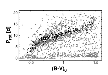
Figure 4: Merged data of the eight clusters after multiplying the cluster periods by the factors given by the exact Skumanich-law (i.e., $P_{\rm tranf}=P_{\rm obs}\sqrt{AGE(\rm M44)/AGE(\rm clus)}$.) The cluster ages are given in Table 1. Data from M44 (Praesepe) are shown by black dots.

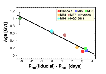
Figure 5: Linear regression of the optimum period shift parameters to the cluster isochrone ages (see Tables 1 and  2 and Eq. (5)). Except for NGC 6811, the estimated errors (both for the isochrone ages and for the period shifts) are smaller or nearly of the size of the dots. The standard deviation of the fit is $0.16$ Gyr.

With the optimum period shifts we are in the position to investigate the functional dependence of the shift on cluster age. An inspection of this plot (see Fig. 5) by eye clearly shows that a simple linear correlation should yield a fairly accurate description of the functional dependence (at least at the current stage, with eight data points at hand). The linear regression yields the following expression and formal error estimate

$${\rm AGE}_{\rm gyro} = a_{0}+a_{1}\Delta P$$

$$\sigma^{2}({\rm AGE}_{\rm gyro}) = K_{11}+K_{22}(\Delta P)^{2}+a_{1}^{2}\sigma^{2}(\Delta P)+2K_{12}\Delta P$$

$$\Delta P = P_{\rm rot}^{\rm fiducial}-P_{\rm rot}$$

$$a_{0} = \,\,\,0.620,\quad\quad a_{1}=-0.138$$

$$K_{11} = \,\,\,0.004682,K_{22}=0.000734$$

$$K_{12} = -0.000978.$$ (5)

The fiducial period $P_{\rm rot}^{\rm fiducial}$ can be easily evaluated for any star given its dereddened color and using Eq. (3). This means that Eq. (5) is directly applicable to the estimation of the gyrochronological age of any star with known color and rotation period. We note that the error formula was derived by assuming a uniform isochrone age error as given by the standard deviation of the fit.

We emphasize that this equation was derived by using the isochrone ages of the calibrating clusters. Therefore, we expect this formula to yield a fair approximation of the isochrone age of any (rotationally settled) target within the calibrating parameter range and hopefully beyond.

It is interesting to compare the derived star-by-star gyro-ages for each cluster with their isochrone ages. The result of this comparison is shown in Fig. 6. Although there are clusters (i.e., M37, M45, NGC 6811) with some observable trend in the run of the individual gyro-ages, the overall fit is satisfactory. This figure also highlights the relatively large errors we may expect when the gyrochronological method is employed on individual targets (even if there was a way to ascertain that they are in the rotationally settled state). For comparison, in Appendix B we show the same plot by using the gyro-age formula of Angus et al. (angus2015 (2015)). Their formula is based on the functional form of period and color dependence of Barnes (barnes2003 (2003)). Because of the multiplicative nature of the age-period dependence, we see larger systematic variations in the estimated ages than in the case of the additive dependence.

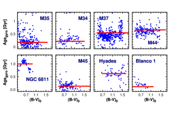
Figure 6: Predicted individual gyro-ages (dots) by using Eqs. (3) and (5) and the adopted isochrone cluster ages of Table 1 (lines).

3 Tests on independent datasets

Although the gyro-age formula derived in Sect. 2 is expected to have a limited applicability, it is important to see how broad this limit is. As mentioned, we cannot investigate whether the stars to be tested are in the rotationally settled state. This, by itself, introduces a great deal of uncertainty. The isochrone ages are also erroneous, sometimes so excessively (e.g., for K and M dwarfs) that individual ages rarely have any value. Nevertheless, such a test (if employed on a sufficiently large sample) may tell us something about the applicability of the gyro-age method and may also shed light on the evolution of the rotation of various stellar populations.

3.1 Bright field stars and the Sun

Valenti & Fisher (valenti2005 (2005)) published accurate spectroscopic parameters (including $v_{\rm rot}\sin i$ values) for over one thousand nearby bright, mostly main-sequence F–K stars. We adopted their isochrone ages (based on the Yonsei-Yale stellar evolution models of Demarque et al. demarque2004 (2004)) and used their mass and gravity values to compute the stellar radii. From these and the rotation velocities, we estimated the rotation periods (in [days]): $P_{\rm rot}=50.6R/(v_{\rm rot}\sin i)$, where the stellar radius $R$ is in solar units and the rotation velocity $v_{\rm rot}\sin i$ is in [kms^-1]. From the effective temperature, gravity, and metallicity given by Valenti & Fisher (valenti2005 (2005)), we can estimate $(B-V)_{0}$ with the aid of the formula of Sekiguchi & Fukugita (sekiguchi2000 (2000))

$$(B-V)_{0} = -813.3175+684.4585\log T_{\rm eff}$$ (6)

$$- 189.923(\log T_{\rm eff})^{2}+17.40875(\log T_{\rm eff})^{3}$$

$$+ 1.2136[Fe/H]+0.0209[Fe/H]^{2}$$

$$- 0.294[Fe/H]\log T_{\rm eff}-1.166\log g$$

$$+ 0.3125\log g\log T_{\rm eff}\hskip 5.69054pt.$$

With these parameters we can evaluate the gyro-age for each star and compare it with the corresponding isochrone age. In a similar representation we can plot the isochrone age as a function of $P_{\rm rot}(\rm fiducial)-P_{\rm rot}$ and compare it with the gyro-age estimate of Eq. (5). In the data preparation we excluded objects with rotational velocities lower than $0.1$ kms^-1 and also those that did not pass our criterion of isochrone fitting (see Sect. 3.3). Finally, we had a sample with $934$ stars from the original sample of $1039$ stars of Valenti & Fisher (valenti2005 (2005)). We also note that for demonstrative purpose we trimmed the period shift$-$age plotting area to the space of interest, thereby excluding some small fraction of objects. This does not affect our conclusion in any way because on the one hand, these objects have extreme parameter values that are largely irrelevant for the effect we investigate, and on the other hand, their observable and derived parameters (e.g., age, rotation period) are also generally inaccurate.

In Fig. 7 we plot the isochrone ages given by Valenti & Fisher (valenti2005 (2005)) as a function of the rotational period shift. For reference, we also overplot the corresponding cluster values. Clearly, there is a striking difference between the isochrone and gyro-ages. Nearly all isochrone ages are greater than the gyro-ages. If we focus only on the more densely populated part of the plot, we see that the overall difference is $2$ Gyr. Unfortunately, the region below $1$ Gyr (where the calibration was performed) is rather sparsely populated. Nevertheless, it seems that even in this regime the isochrone ages carry the same property as in the non-calibrated (older age) regime. We note that correcting the spectroscopic rotation velocities for the overall aspect effect (e.g., Nielsen et al. nielsen2013 (2013)) exacerbates the situation because it leads to higher rotational velocities, shorter periods, and therefore to even younger gyro-ages. Furthermore, possible systematic bias in the rotation velocities might occur at low-rotation rates when the rotational broadening is similar to other broadening effects (e.g., stellar macroturbulence). However, these stars do not contribute in an important way to the discrepancy above, since more than half of the sample has $v\sin i>2$ km^-1.

The case of the Sun is special because we know both its age and its rotation period, together with other physical parameters. Taking the equatorial rotation period, we derive that the gyro-age of the Sun is $3.74\pm 0.65$ Gyr. Again, the gyro-age is $0.9$ Gyr short relative to the accurately known age of $4.6$ Gyr (which happens to be close to the actually computed isochrone age of $4.4$ Gyr, based on the Yonsei-Yale models discussed in Sect. 3.3.)

To show that this age discrepancy is not unique for the additive period$-$age scaling introduced in this paper, we applied two different period$-$color$-$age calibrations on the above dataset. The result (presented in Appendix B) clearly shows that the discrepancy is generic.

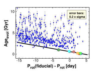
Figure 7: Period shift vs. evolutionary (i.e., isochrone) ages for the field star sample of Valenti & Fisher (valenti2005 (2005)) (blue dots) and for the eight open cluster ridges as presented in this paper (large colored dots). The linear regression to the cluster data is shown by the black line.

3.2 Transiting extrasolar planet host stars

The host stars of extrasolar planets are usually very deeply studied objects because it is important to accurately determine the stellar parameters to derive the planet parameters. In addition, if the planet is also transiting planet, the average stellar density is rather tightly constrained by the basic orbital parameters of the planet (Seager & Mallén-Ornelas seager2003 (2003); Sozzetti et al. sozzetti2007 (2007)). As a result, these stars are very useful targets for testing the gyro-age method.

We compiled the relevant physical parameters of $147$ bright transiting planet host stars from the literature. All of these systems have been discovered by ground-based surveys. All ages used are stellar model (isochrone) ages, and they have been derived mainly from the Yonsei-Yale models. Unfortunately, the rotation periods are still based on the spectroscopic $v_{\rm rot}\sin i$ values, since there are rather few host stars with reliable direct photometric rotation periods.

The result is plotted in Fig. 8 in the same fashion as before. Unfortunately, some stars, otherwise possessing accurately determined stellar parameters, had to be omitted because of their extreme parameters. For instance, WASP-33 is a rare A-type host star, with a high rotation rate of $90$ kms^-1, yielding a $P_{\rm rot}$ value of $0.79$ days. The isochrone age is fairly well constrained with an upper limit of $0.4\pm 0.3$ Gyr (Collier Cameron et al. collier2010 (2010); Kovács et al. kovacs2013 (2013)). Although the fast rotation is consonant with its young age, we cannot verify this with our gyro-age formula because the target is outside its validity. For similar reasons we excluded five stars. As in the test of the Valenti & Fisher (valenti2005 (2005)) dataset, we also focus on a limited area of the period shift$-$age space (and again, only a small fraction of objects were excluded, which does not alter our conclusion).

Although the data are sparser than for the large nearby star survey of Valenti & Fisher (valenti2005 (2005)), the same effect is still well visible: the highly significant excess of stars dated older by the isochrone age determination. With the overall more accurate isochrone ages for these bright, well-studied stars, the discrepancy between the two types of age determination is reaffirmed.

Similarly to the test presented on the Valenti & Fisher (valenti2005 (2005)) dataset in Sect. 3.1, here we refer to Appendix B, where we compare our gyro-ages with those recently derived by Maxted et al. (maxted2015 (2015)) on a sample of limited-number extrasolar host stars with measured rotation periods. In spite of our very different approach, the two types of gyro-ages correlate very well, supporting their conclusion on the shorter gyro-ages for their planet host sample.

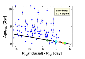
Figure 8: As in Fig. 7, but for the sample of hot-Jupiter host stars, discovered by ground-based surveys.

3.3 Rotational variables from the Kepler field

A large sample of rotational variables have recently been identified by McQuillan, Mazeh & Aigrain (mcquillan2014 (2014)) through analyzing the photometric database of the Kepler satellite. This includes all possible rotational variables in the Kepler field. In an earlier publication, McQuillan, Mazeh & Aigrain (mcquillan2013 (2013)) investigated only those targets that were labeled as Kepler objects of interest (KOI). Here we focus on this smaller sample, containing 760 objects. A negligible fraction ($5$%) of this sample contains probable eclipsing binaries, blends, or suffers from other ambiguities.

Employing these KOI targets in our tests has the advantage of using photometric rotation periods instead of spectroscopic ones, thereby substantially decreasing the additional source of scatter due to the aspect angle dependence. However, there is also a drawback of using these data. Since the Kepler targets are numerous and have considerably lower apparent brightness, their basic spectroscopic and photometric parameters are usually less accurate than those of the individually studied bright planet host stars.

Since the published data do not contain evolutionary (or any) age information, we computed isochrone ages according to the Yonsei-Yale models (Demarque et al. demarque2004 (2004)). With the aid of their interpolation routine and additional fine-grid interpolation, we established a dense isochrone grid for solar-scaled models without $\alpha$ element enhancement. The metallicity and age grids are uniform and cover the following values: $\{Z_{i}=0.001+(i-1)0.0005;i=1,2,...,80\}$ and $\{\log t_{j}=8.00+(j-1)0.02;\text{}j=1,2,...,107\}$. Each of the downloaded isochrone contains $140$ $(\log T_{\rm eff},\log g)$ mesh points that we further increased by linear interpolation to $\sim 560$, leading to sufficiently dense sampling in all parameters to be matched to the spectroscopic data. The solar heavy element abundance for these models is equal to $0.018$. We minimized the following metric to select the best matching models

$$D^{2}=w(\Delta\log T_{\rm eff})^{2}+(1-w)(\Delta\log g)^{2}\hskip 5.69054pt,$$ (7)

where $\Delta$ stands for the difference between the grid point and the observed values. The weight $w$ was chosen to be $5/6$ and takes into consideration the smaller range of $logT_{\rm eff}$ values entering the matching procedure. For the observed values falling within the region spanned by the isochrones, we derived matching distances $D$ lower than $0.002$, usually close to $0.001$ or lower (indicating that we have a sufficiently densely interpolated set of models). We obtained a rough estimate on the error of the age by computing the standard deviation of all model values satisfying the $D<0.04$ criterion. This rather high cutoff for $D$ is set for the broad agreement of our error estimates with those found in the literature. In computing $\sigma({\rm age})$, the standard deviation of the ages satisfying the condition posed by $D$, we weighted the various age values by the inverse of the square of the corresponding distances

$$\sigma^{2}({\rm age})=\sum_{\rm k=1}^{n}w_{k}({\rm age}_{k}-\langle{\rm age}\rangle)^{2}\hskip 5.69054pt,$$ (8)

where $w_{k}=(1/D_{k}^{2})/\sum_{\rm j=1}^{n}1/D_{j}^{2}$ and $n$ is the total number of grid points satisfying the $D<0.04$ criterion, and $D_{j}$ is the distance $D$ (see Eq. (7)) of the j-th grid point from the target values. The average age $\langle{\rm age}\rangle$ was computed in a similar manner: $\langle{\rm age}\rangle=\sum_{\rm k=1}^{n}w_{k}{\rm age}_{k}$. (We note that in the tests we used the best-fitting model value as our age estimate rather than this average.) In a comparison with the ages found in the literature on the sample of hot-Jupiter host stars (Sect. 3.2), we found that except for a few outliers at young or old ages and for some $20$% of stars with deviations $0.5$–$1.5$ Gyr, this simple fitting method yields ages that agree well with the published values within $\pm 0.5$ Gyr. (See also Appendix B for an example of this compatibility on a small size of sample of hot Jupiters compiled by Maxted et al. maxted2015 (2015).)

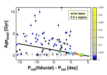
Figure 9: As in Fig. 7, but for the KOI sample of McQuillan, Mazeh & Aigrain (mcquillan2013 (2013)). The evolutionary ages were computed with the aid of the Yonsei-Yale isochrones. The high-density horizontal set of points at low isochrone ages dominantly constitutes stars with observed stellar parameters outside the isochrone regime. The color coding is scaled by the best isochrone matching distance (Eq. (7)) and shows that most of these low-lying stars do not match the isochrones.

For the $762$ stars of McQuillan, Mazeh & Aigrain (mcquillan2013 (2013)) we used the spectroscopic and photometric parameters recently revised by Huber et al. (huber2014 (2014)). To discard suspected items with excessive errors, we performed a fairly generous parameter cut by requiring both the [Fe/H] and the $\log g$ errors to be smaller than $0.2$. This filtering led to a sample of $207$ stars that was further decreased to $204$ by satisfying the condition of $D<0.04$.

The resulting period$-$age plot is shown in Fig. 9. The plot is very similar to the earlier ones, showing the significantly older ages obtained from the isochrone fits. In addition to this general feature, we also recognize a relatively large number of young (looking) objects with nearly the same age of $0.1$–$0.3$ Gyr. As the side bar shows, most of these objects have rather low isochrone matching accuracy (i.e., they have high $D$ values). Indeed, a comparison with the $\log T_{\rm eff}-\log g$ isochrone plot shows that nearly all of these objects are outside the regime covered by the isochrones for the given metallicity. More specifically, their spectroscopic gravity is higher than expected from the models. If we discard these objects, the trend toward greater isochrone ages is again clear.

4 Conclusions

The purpose of this paper was threefold: i) examine the validity of the Skumanich-type scaling between the stellar rotation period, color, and age through a comprehensive analysis of the available observations on open clusters; ii) compare the ages based on the revised scaling with the stellar evolutionary (isochrone) ages for various samples of stars; and (iii) if the result of test (ii) is positive (i.e., no major discrepancy is found), recalibrate the gyro-age formula to accommodate the older ages and different evolutionary histories of these samples and thereby make the age determination based on stellar rotation more widely applicable.

In test (i) we compiled the data from eight open clusters and searched for a simple transformation that generates a tight relation between the color and rotation period for the full sample. As has previously been indicated but left untreated in some other publications – for example, Cargile et al. cargile2014 (2014), by using the Skumanich-type multiplicative period transformation, the periods are stretched too much at the long-period side (i.e., toward lower mass stars), leading to a rather fuzzy color$-$period plot when all data are combined. If we instead use a simple additive scaling (i.e., we shift the periods by cluster-dependent optimal constants), then the individual cluster ridges align in a much tighter way. This enabled us to investigate the relation between cluster ages and period shifts on a more solid statistical basis. The relation between these two quantities was also fairly tight, which together with the derived fiducial ridge (expressing the relation between the color and period for rotationally settled near main-sequence F–K dwarfs at a given age) enabled us to give age estimates for other stars based on their rotation periods and colors (see Eqs. (3) and (5)).

It is not the purpose of this paper to discuss the possible theoretical consequences of the better fitting additive period$-$age scaling. Here we only note three aspects that should be considered in constructing a revised model of stellar angular momentum dissipation. First, the rotational evolution of stars in open clusters might differ from those in the field due to the substantially different stellar environment and the low density of interstellar matter. Second, the rate of angular momentum loss is a strong function of the assumed structure of magnetic field and other physical details (e.g., core-envelope coupling, magnetic field strength vs. rotation, etc.) For example, Reiners & Mohanty (reiners2012 (2012)) derived a rotation-rate dependence of $t^{-1/4}$ in the non-saturated regime for $1M_{\odot}$ stars merely by adopting a different physical meaning of the magnetic flux – rotation rate relation. Third, both the sample size and the age range of open clusters available currently for gyro-age studies are small, therefore the true age$-$rotational period relation might be more involved than the one derived here. (We sampled only a small part of an unknown function that was incidentally best approximated by a linear relation in this restricted parameter space.)

Test (ii) resulted in a negative conclusion for all three datasets (field stars, host stars of transiting hot Jupiters, and Kepler planetary candidate stars). The bulk of the isochrone ages is $1.5$–$2.0$ Gyr greater than the predicted gyro-ages, with a large scatter to even larger differences. Only a small fraction of stars show younger isochrone ages in all three samples. It is important to recall that the ages of the open clusters – which the gyro-ages have been calibrated to – are also based on isochrone ages, essentially on the same evolutionary stellar models, as those used in the test samples. Although the age overlap between the field stars and open cluster stars is not too extensive, it seems that the above difference is characteristic for all ages, also including the younger age range of the calibrating clusters. Therefore, the discrepancy does not seem to be the result of a poor extrapolation of the age relation derived from open clusters. Although the topology of the isochrones may introduce some bias toward older ages, this effect is likely to be small, based on the survival of the age discrepancy for stars with accurate isochrone ages (e.g., Sun, KELT-2A – see Beatty et al. beatty2012 (2012)). Apparently, non-cluster field stars have significantly lower slow-down rates than their cluster counterparts.

This study supports the conclusions of other current works investigating the performance of the gyro-age method on various stellar populations. From the study of bright planet host stars, Maxted, Serenelli, & Southworth (maxted2015 (2015)) reached the same conclusion as we did, in spite of their quite different gyro-age method. Earlier, Brown (brown2014 (2014)) also found hints of the young gyro-ages of extrasolar planet host stars. Based on a Monte Carlo study of a large sample of Kepler asteroseismic targets and data from two open clusters, Angus et al. (angus2015 (2015)) also questioned the overall reliability of the current gyro-age estimations.

In these circumstances, we were obviously unable to pursue task (iii). A more reliable extension of the gyro-age method to non-cluster stars should probably wait until the source of the discrepancy between the current gyro- and isochrone ages of the field and cluster stars is understood and a physically acceptable solution is found. Finally, we note that our conclusion is based on isochrone ages derived from non-rotating stellar evolutionary models. Brandt & Huang (brandt2015 (2015)) recently showed that with rotating models the age of the Hyades and Praesepe clusters become considerably older (from the generally accepted value of 630/670 Myr – which we also used here – to $\sim 800$ Myr). An extension of the evolutionary models in this direction might mitigate some part of the discrepancy we highlighted here.

Appendix A Fiducial polynomial and the robust fit of the ‘I’ sequences

To find the best representation of the joint ‘I’ sequences of the merged data of Praesepe (M44) and the Hyades, we fitted polynomials of various order and checked the fit both by visual and by statistical means. We omitted the obvious outliers that are mostly due to the rotationally unsettled lower temperature stars in the Hyades (we note that all outliers are well defined). Altogether, we left out two stars from Praesepe and $11$ from the Hyades and compiled a sample of $228$ stars. These stars were fitted by least squares of equal weights. Figure 10 shows the variation of the unbiased estimate of the standard deviation of the residuals as a function of the polynomial order.

The standard deviation levels off at about order four. Although there is some decrease afterward, the fit shows wiggles with increasing amplitudes as the order of the polynomial increases. The fit starts to become unstable at order nine, and it becomes entirely volatile at order ten with a residual standard deviation of $4.1$. We also tested the statistical significance of the fourth-order fit by using the following statistics

$$R(j_{1},j_{2}) = \left({{RSS(j_{1})}\over{RSS(j_{2})}}-1\right){{n-j_{2}}\over{j_{2}-j_{1}}}$$

$$RSS_{k} = \sum_{i=1}^{n}(P_{rot}(i)-p_{k}(i))^{2}\hskip 5.69054pt.$$ (9)

Here $n$ is the number of data points, $\{p_{k}(i)\}$ is the fitted polynomial of order $k$, and $j_{1}$ and $j_{2}$ are the order tested. In our case, $j_{2}=j_{1}+1$, so $R(j_{1},j_{2})$ follows a Fisher distribution of $F(1,n-j_{2})$. We assessed the significance of the change in $R(j_{1},j_{2})$ in terms of the theoretical standard deviation of $F(1,n-j_{2})$. This yields some $8\sigma$ significance at each step for the change in $R(j_{1},j_{2})$ as we go from the second- to the fourth-order fits. After this, the significance decreases to $\sim 2\sigma$ with an increase at order eight and then the solution becomes unstable, as mentioned.

The fourth-order polynomial fitted to the merged data of M44 and the Hyades is shown in Fig. 11. The regression parameters and their statistical errors are given by Eq. 3.

This fiducial polynomial was used in Sect. 2.2 to derive the relative period shifts of the ‘I’ sequences of the individual clusters. The best-fit shifts were determined by using a kernel-weighted least-squares method to consider outliers (i.e., minimizing the effect of stars not associated with the ‘I’ sequence). The kernel proposed by German & McClure (german1987 (1987)) has proven to be an excellent way of localizing the ridge in each cluster. We show an example for the robustness of the fit in Fig. 12.

Figure 10: Polynomial order vs. unbiased estimate of the standard deviation of the residuals of the fit for the fiducial ridge fitting (see Fig. 11). For reference, the horizontal line shows to the standard deviation at order four.

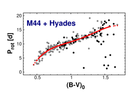
Figure 11: Fourth-order polynomial fit to the combined data of M44 (Praesepe, gray points) and the Hyades (black points). The fit (red dots) is sampled at the same $(B-V)_{0}$ values as the data. All data are plotted, including the $13$ outliers mentioned in the text.

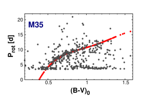
Figure 12: Result of the best-fit period shift of the rotation periods of M35 (gray dots) to the fiducial ridge (red dots) by using the GM kernel (German & McClure german1987 (1987)). The fiducial ridge is sampled at the same $(B-V)_{0}$ values as the data.

Appendix B Comparison with other studies

First we calculated the individual rotational ages of the cluster sample used in this paper by employing the gyro-age formula of Angus et al. (angus2015 (2015)). Their Eq. (15) has the standard form as introduced by Barnes (barnes2003 (2003)), but the parameters are determined by using $310$ astroseismic targets from the survey of the Kepler satellite and some additional stars from the field and from some open clusters. We plot the individual gyro-ages for the eight clusters in Fig. 13. In comparison with Fig. 6, using our additive age-period-color relation, the ages corresponding to the stars associated with the ridges of type ‘I’ have stronger systematic variations than those derived from our additive formula (see, e.g., the plot for M37). This is the effect of multiplicative period–age scaling, as discussed in Sect. 2.

In the rest of this appendix we show that the significantly younger rotational ages derived for the field stars from our newly calibrated additive formula is not specific to this formula, but is a general property of all currently used gyro-age calibrations.

In the lower panel of Fig. 14 we plot the evolutionary ages as given in the spectroscopic survey of $1039$ field stars by Valenti & Fisher (valenti2005 (2005)) vs. the rotational ages derived from one of the most frequently used gyro-age formula of Barnes (barnes2007 (2007), his Eq. (1)). For comparison, in the upper panel of the same figure we show the plot derived from the additive gyro-age formula presented in this paper. In both cases we use a subsample of the full survey as described in Sect. 3.1.

Although different in details, the two plots are topologically closely similar, indicating in both cases a significant excess of old evolutionary ages. The high density of points in the [0,5] Gyr regime suggests an overall difference of 1–2 Gyr. From the color-coded radius distribution it is also clear that differences much higher than the quoted value exist for stars with lower radii. By repeating the iso-gyro age comparison for other empirical gyro-age formulae – that is, those of Mamajek & Hillenbrand (mamajek2008 (2008)) (their Eqs. (12)–(14) with the parameters given in their Table (10)) and Angus et al. (angus2015 (2015)) (their Eq. (15)) – a similar conclusion can be drawn on the topology of the gyro- vs. evolutionary age relation. Interestingly, these two works yield very similar parameters for the Barnes-type gyro-age relation, in spite of the very different input data and methods of analysis, and the conclusion of the authors in the second paper about the limited applicability of the formulae presented for the full population of the dataset used in the calibration.

Yet another approach for estimating gyro-ages comes from the analytical model of Barnes (barnes2010 (2010), see also Barnes & Kim barnes-kim2010 (2010)). Maxted et al. (maxted2015 (2015)) employed this model to analyze $28$ well-established extrasolar planet host stars with measured photometric rotation periods. We employed this sample with the stellar parameters used in their paper to compute our age estimates. The plots in Fig. 15 show the excellent correlations between the ages of Maxted et al. (maxted2015 (2015)) and those presented here. This good agreement is rather surprising for the gyro-ages, since our ages are basically empirical (with the intermediation of the cluster ages determined by the stellar evolutionary isochrone fits), whereas their ages are more involved through various model approximations and initial conditions. For the evolutionary ages there is a uniform shift of $0.5$–$1$ Gyr in the sense that the ages computed by Maxted et al. (maxted2015 (2015)) are older than ours. This tendency of the garstec models of Weiss & Schlattl (weiss2008 (2008)) used by Maxted et al. (maxted2015 (2015)) was also noted by Metcalfe et al. (metcalfe2014 (2014)). Chaplin et al. (chaplin2014 (2014)) attributed this offset to the different treatment of convective core overshooting in the garstec models.

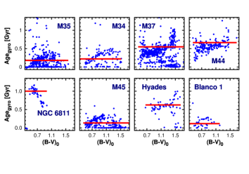
Figure 13: Predicted individual gyro-ages (dots) by using the formula of Angus et al. (2015) and the adopted isochrone cluster ages of Table 1 (lines).

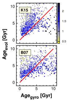
Figure 14: Rotational ages vs. stellar evolution ages computed using the additive gyro-age formula Eq. (5) derived in this paper (upper panel) and the popular multiplicative formula of Barnes (barnes2007 (2007)) (lower panel). The thick continuous lines indicate the identical values of the rotational and evolutionary ages. We use the spectroscopic data of Valenti & Fisher (valenti2005 (2005)). The color coding is for the stellar radius as indicated by the side bar (scaled in solar units).

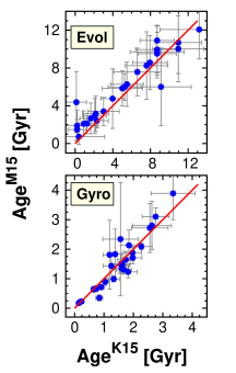
Figure 15: Comparison of the evolutionary ages (upper panel) and the rotational ages (lower panel) for the extrasolar planet host stars of Maxted et. al (maxted2015 (2015)) with those derived in this paper using the Yonsei-Yale isochrones of Demarque et al. (demarque2004 (2004)) and the additive gyro-age formula Eq. (5) of this paper. The continuous line indicates the identical values for the quantities corresponding to the labels. We note that the panels have different ranges.