Uniform Asymptotic Inference and the Bootstrap After Model Selection

Abstract

Recently, Tibshirani et al. (2016) proposed a method for making inferences about parameters defined by model selection, in a typical regression setting with normally distributed errors. Here, we study the large sample properties of this method, without assuming normality. We prove that the test statistic of Tibshirani et al. (2016) is asymptotically valid, as the number of samples $n$ grows and the dimension $d$ of the regression problem stays fixed. Our asymptotic result holds uniformly over a wide class of nonnormal error distributions. We also propose an efficient bootstrap version of this test that is provably (asymptotically) conservative, and in practice, often delivers shorter intervals than those from the original normality-based approach. Finally, we prove that the test statistic of Tibshirani et al. (2016) does not enjoy uniform validity in a high-dimensional setting, when the dimension $d$ is allowed grow.

1 Introduction

There has been a recent surge of work on conducting formally valid inference in a regression setting after a model selection event has occurred, see Berk et al. (2013); Lockhart et al. (2014); Tibshirani et al. (2016); Lee et al. (2016); Fithian et al. (2014); Bachoc et al. (2014), just to name a few. Our interest in this paper stems in particular from the work of Tibshirani et al. (2016), who presented a method to produce valid p-values and confidence intervals for adaptively fitted coefficients from any given step of a sequential regression procedure like forward stepwise regression (FS), least angle regression (LAR), or the lasso (the lasso is meant to be thought of as tracing out a sequence of models along its solution path, as the penalty parameter descends from $\lambda=\infty$ to $\lambda=0$). These authors use a statistic that is carefully crafted to be pivotal after conditioning on the model selection event. This idea is not specific to the sequential regression setting, and is an example of a broader framework that we might call selective pivotal inference, applicable in many other settings, as in, e.g., Taylor et al. (2016); Lee et al. (2016); Lee & Taylor (2014); Loftus & Taylor (2014); Reid et al. (2017); Choi et al. (2014); Fithian et al. (2014); Hyun et al. (2016).

A key to the methodology in Tibshirani et al. (2016) (and much of the work in selective pivotal inference) is to the assumption of normality of the errors. To fix notation, consider the regression of a response $Y\in\mathbb{R}^{n}$ on predictor variables $X_{1},\ldots,X_{d}\in\mathbb{R}^{n}$, stacked together as columns of a matrix $X\in\mathbb{R}^{n\times d}$. We will treat the predictors $X$ are fixed (nonrandom), and assume the model

$$Y_{i}=\theta_{i}+\epsilon_{i},\;\;\;i=1,\ldots,n,$$ (1)

where $\theta\in\mathbb{R}^{n}$ is an unknown mean parameter of interest. Tibshirani et al. (2016) assume that the errors $\epsilon_{1},\ldots,\epsilon_{n}$ are i.i.d. $N(0,\sigma^{2})$, where the error variance $\sigma^{2}>0$ is known. An advantage of their approach is that it does not require $\theta$ to be an exact linear combination of the predictors $X_{1},\ldots,X_{d}$, and makes no assumptions about the correlations among these predictors. But as far as the finite-sample guarantees are concerned, normality of the errors is crucial. In this work, we examine the properties of the test statistic proposed in Tibshirani et al. (2016)—hereafter, the truncated Gaussian (TG) statistic—without using an assumption about normal errors. We only assume that $\epsilon_{1},\ldots,\epsilon_{n}$ are i.i.d. from a distribution with mean zero and essentially no other restrictions.

A high-level description of the selective pivotal inference framework for sequential regression is as follows (details are provided in Section 2). FS, LAR, or the lasso is run for some number of steps $k$, and a model is selected, call it $M$. For FS and LAR, this model will always have $k$ active variables, and for the lasso, it will have at most $k$, as variables can be added to or deleted from the active set at each step. We specify a linear contrast of the mean $v^{T}\theta$ of interest, e.g., one giving the coefficient of a variable of interest in the model $M$ at step $k$, in the regression of $\theta$ onto the active variables. By assuming normal errors in (1), and examining the distribution of $v^{T}Y$ conditional on having selected model $M$, which we denote by $\widehat{M}(Y)=M$, we can construct a confidence interval $C_{\alpha}$ satisfying

$$\mathbb{P}\Big{(}v^{T}\theta\in C_{\alpha}\,\Big{|}\,\widehat{M}(Y)=M\Big{)}=1-\alpha,$$

for a given $\alpha\in[0,1]$. The interpretation: if we were to repeatedly draw $Y$ from (1) and run FS, LAR, or the lasso for $k$ steps, and only pay attention to cases in which we selected model $M$, then among these cases, the constructed intervals $C_{\alpha}=C_{\alpha}(Y;M)$ contain $v^{T}\theta$ with frequency tending to $1-\alpha$.

The above is a conditional perspective of the selective pivotal inference framework for FS, LAR, and lasso. An unconditional or marginal point of view is also possible, which we now describe. For each possible selected model $M$, a constrast vector $v_{M}$ is specified, and the contrast $v_{M}^{T}\theta$ is considered when model $M$ is selected, $\widehat{M}(Y)=M$. To be concrete, we can again think of a setup such that $v_{M}^{T}\theta$ gives the coefficient of a variable in the model $M$ at step $k$, in the projection of $\theta$ onto the active set. Confidence intervals are then constructed in exactly the same manner as above (without change), and conditional coverage over all models $M$ implies the following unconditional property for $C_{\alpha}$,

$$\mathbb{P}\Big{(}v_{\widehat{M}(Y)}^{T}\theta\in C_{\alpha}\Big{)}=1-\alpha.$$

The interpretation is different: if we were to repeatedly draw $Y$ from (1) and run FS, LAR, or lasso for $k$ steps, and construct confidence intervals $C_{\alpha}=C_{\alpha}(Y;\widehat{M}(Y))$, then these intervals contain their respective targets $v_{\widehat{M}(Y)}^{T}\theta$ with frequency approaching $1-\alpha$. Notice that, by construction, the target itself may change each time we draw $Y$, though it is the same for all $Y$ that give rise to the same selected model. In terms of the setting for regression contrasts described above, each time we draw $Y$ and carry out the inferential procedure, the interval $C_{\alpha}$ covers the coefficient of a possibly different variable in the active model, in the projection of $\theta$ onto the active variables. Figure 1 demonstrates this point.

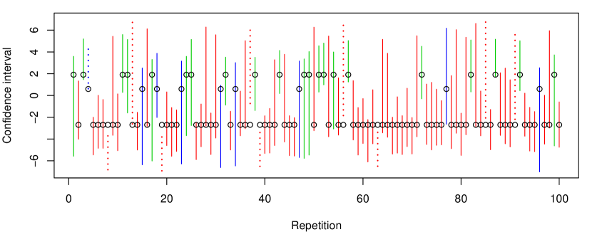
Figure 1: An example of conditional and unconditional coverage for one step of FS (the variables are normalized, and this is equivalent to one step of LAR, or lasso). Here $n=20$ and $d=3$, and a response $Y$ was drawn 100 times from a model as in (1) with i.i.d. $N(0,\sigma^{2})$ errors. The different colors denote different active models that were selected after one step, where an active model is a variable-sign pair, namely, the variable achieving the largest absolute inner product with $Y$, and the sign of this inner product. Across the 100 repetitions, the circles denote a target to be covered, and the segments are 90% confidence intervals. E.g, the color green corresponds to the model $+X_{2}$, so in repetitions 1, 3, 11, 12, etc., $X_{2}^{T}Y$ was largest among all absolute inner products of variables with $Y$, and the green segments denote 90% confidence intervals designed to cover the contrast $X_{2}^{T}\theta$. Similarly, red corresponds to the model $-X_{1}$, and blue to $+X_{3}$. Dotted segments indicate that the given interval does not cover its target. The empirical coverage among green intervals: 21/21, among red intervals: 61/70, and among blue intervals: 8/9. Hence in each case, the empirical coverage is close to the nominal 90% level. Further, in total, i.e., unconditionally, the empirical coverage is 90/100, right at the nominal 90% level.

1.1 Uniform convergence

When making asymptotic inferential guarantees, as we do in this paper, it is important to be clear about the type of guarantee. Here we review the concepts of uniform convergence and validity. Let $\xi_{1},\ldots,\xi_{n}\in\mathbb{R}^{s}$ be random vectors with joint distribution $(\xi_{1},\ldots,\xi_{n})\sim F_{n}$, where $F_{n}\in\pazocal{P}_{n}$, and $\pazocal{P}_{n}$ is a class of distributions. For example, we could have $\xi_{1},\ldots,\xi_{n}\in\mathbb{R}^{s}$ i.i.d. from $F$, and the class $\pazocal{P}_{n}$ could contain product distributions of the form $F_{n}=F\times\ldots\times F$ ($n$ times); our notation allows for a more general setup than this one. Let $W_{n}=T_{n}(\xi_{1},\ldots,\xi_{n})$ for a statistic $T_{n}$, and $W\sim G$, where $W_{n},W\in\mathbb{R}^{q}$. We will say that $W_{n}$, converges uniformly in distribution to $W$, over $\pazocal{P}_{n}$, provided that

$$\lim_{n\to\infty}\;\sup_{F_{n}\in\pazocal{P}_{n}}\;\sup_{x\in\mathbb{R}^{q}}\;\big{|}\mathbb{P}_{F_{n}}(W_{n}\leq x)-\mathbb{P}(W\leq x)\big{|}=0.$$ (2)

(The above inequalities, as in $W_{n}\leq x$ and $W\leq x$, are meant to be interpreted componentwise; we are also implicitly assuming that the limiting distribution $G$ is continuous, otherwise the above inner supremum should be restricted to continuity points $x$ of $G$.) This is much stronger than the notion of pointwise convergence in distribution, which only requires that

$$\lim_{n\to\infty}\;\sup_{x\in\mathbb{R}^{q}}\;\big{|}\mathbb{P}_{F_{n}}(W_{n}\leq x)-\mathbb{P}(W\leq x)\big{|}=0,$$ (3)

for a particular sequence of distributions $F_{n}$, $n=1,2,3,\ldots$.

A recent article by Kasy (2015) emphasizes the importance of uniformity in asymptotic approximations. This authors points out that a uniform version of the continuous mapping theorem follows directly from a standard proof of the continuous mapping theorem (e.g., see Theorem 2.3 in van der Vaart (1998)).

Lemma 1.

Suppose that $W_{n}$ converges uniformly in distribution to $W$, with respect to the class $\pazocal{P}_{n}$. Let $\psi:\mathbb{R}^{q}\to\mathbb{R}$ be a map that is continuous on a set $D$, such that $\mathbb{P}(W\in D)=1$. Then $\psi(W_{n})$ converges uniformly in distribution to $\psi(W)$ with respect to $\pazocal{P}_{n}$.

Kasy (2015) also remarks that the central limit theorem for triangular arrays, specifically the Lindeberg-Feller central limit theorem (e.g., Proposition 2.27 in van der Vaart (1998)) naturally extends to the uniform case. The logic is, roughly speaking: uniform convergence in (2) is equivalent to pointwise convergence over all sequences of distributions $F_{n}$, $n=1,2,3,\ldots$, and triangular arrays, by design, can have a different distribution assigned to each row. Therefore if the Lindeberg condition holds for any possible sequence, then so does the convergence to normality.

Lemma 2.

Let $\xi_{1},\ldots,\xi_{n}\in\mathbb{R}^{q}$ be a triangular array of independent random vectors, with joint distribution $F_{n}$. Assume $\xi_{1},\ldots,\xi_{n}$ have mean zero and finite variance. Also assume that for any sequence $F_{n}\in\pazocal{P}_{n}$, $n=1,2,3,\ldots$, we have

$$\lim_{n\to\infty}\;\sum_{i=1}^{n}\mathbb{E}_{F_{n}}\Big{(}\|\xi_{i}\|_{2}^{2}\cdot 1\{\|\xi_{i}\|_{2}\geq\epsilon\}\Big{)}=0,\;\;\;\text{for all $\epsilon>0$},$$

and

$$\lim_{n\to\infty}\;\sum_{i=1}^{n}\mathrm{Cov}_{F_{n}}(\xi_{i})=\Sigma,$$

where $\Sigma$ does not depend on the sequence $F_{n}$, $n=1,2,3,\ldots$. Then $W_{n}=\sum_{i=1}^{n}\xi_{i}$ converges in distribution to $W\sim N(0,\Sigma)$, uniformly with respect to $\pazocal{P}_{n}$.

In our work, a motivating reason for the study of uniform convergence is the associated property of uniform validity of asymptotic confidence intervals. That is, if $W_{n}=W_{n}(\mu)$ depends on a parameter $\mu=\mu(F_{n})$ of the distribution $F_{n}$, but $W$ does not, then we can consider any $(1-\alpha)$ confidence set $C_{n,\alpha}$ built from a $(1-\alpha)$ probability rectangle $R_{\alpha}$ of $W$,

$$C_{n,\alpha}=\{\mu:W_{n}(\mu)\in R_{\alpha}\},$$

and the uniform convergence of $W_{n}$ to $W$, really just by rearranging its definition in (2), implies

$$\lim_{n\to\infty}\;\sup_{F_{n}\in\pazocal{P}_{n}}\;\sup_{\alpha\in[0,1]}\;\Big{|}\mathbb{P}_{F_{n}}\Big{(}\mu(F_{n})\in C_{n,\alpha}\Big{)}-(1-\alpha)\Big{|}=0.$$ (4)

Meanwhile, pointwise convergence as in (3) only implies

$$\lim_{n\to\infty}\;\sup_{\alpha\in[0,1]}\;\Big{|}\mathbb{P}_{F_{n}}\Big{(}\mu(F_{n})\in C_{n,\alpha}\Big{)}-(1-\alpha)\Big{|}=0,$$ (5)

for a particular sequence $F_{n}$, $n=1,2,3,\ldots$. For a confidence set satisfying (4), and a given tolerance $\epsilon>0$, there exists a sample size $n(\epsilon)$ such that the coverage is guaranteed to be at least $1-\alpha-\epsilon$, for $n\geq n(\epsilon)$, no matter the underlying distribution (over the class of distributions in question). Note that this is not necessarily true for a pointwise confidence set as in (5), as the required sample size here could depend on the particular distribution under consideration.

1.2 Summary of main results

An overview of our main contributions is as follows.

1. We establish that TG statistics for typical inferences along the FS, LAR, and lasso paths only depend on the data $(X,Y)$ through $\frac{1}{n}X^{T}X$ and $\frac{1}{\sqrt{n}}X^{T}Y$ (Lemmas 3, 4, and 5 in Section 3), which is important since these two quantities have asymptotic limits in a standard low-dimensional asymptotic setup.

2. Placing mild constraints on the mean and error distribution in (1), and treating the dimension $d$ as fixed, we prove that the TG test statistic is asymptotically pivotal, converging to $U(0,1)$ (the standard uniform distribution), when evaluated at the true population value for its pivot argument. We show that this holds uniformly over a wide class of distributions for the errors, without any real restrictions on the predictors $X$ (first part of Theorem 7 in Section 4).

3. The resulting confidence intervals are therefore asymptotically uniformly valid, over the same class of distributions (second part of Theorem 7 in Section 4).

4. The above asymptotic results assume that the error variance $\sigma^{2}$ is known, so for $\sigma^{2}$ unknown, we propose a plug-in approach that replaces $\sigma^{2}$ in the TG statistic with a simple estimate, and alternatively, an efficient bootstrap approach. Both allow for conservative asymptotic inference (Theorem 11 in Section 5).

5. We present detailed numerical experiments that support the asymptotic validity of the TG p-values and confidence intervals for inference in low-dimensional regression problems that have nonnormal errors (Section 6). Our experiments reveal that the plug-in and bootstrap versions also show good performance, and the bootstrap method can often deliver substantially shorter intervals than those based directly on the TG statistic.

6. Our experiments also also suggest that the TG test statistic (and plug-in, bootstrap variants) may be asymptotically valid in even broader settings not covered by our theory, e.g., problems with heteroskedastic errors and (some) high-dimensional problems.

7. We prove that TG statistic does not exhibit a general uniform convergence to $U(0,1)$ when the dimension $d$ is allowed to increase (Theorem 12 in Section 7).

1.3 Related work

A recent paper by Tian & Taylor (2017) is very related to our work here. These authors examine the asymptotic distribution of the TG statistic under nonnormal errors. Their main result proves that the TG statistic is asymptotically pivotal, under some restrictions on the model selection events in question. We view their work as providing a complementary perspective to our own: they consider a setting where the dimension $d$ grows, but place strong regularity conditions on the selected models; we adopt a more basic setting with $d$ fixed, and prove more broad uniformly valid convergence results for the TG pivot, free of regularity conditions.

In a sequence of papers, Leeb & Potscher (2003, 2006, 2008) prove that in a classical regression setting, it is impossible to find the distribution of a post-selection estimator of the underlying coefficients, even asymptotically. Specifically, they prove for an estimate $\widehat{\beta}$ of some underlying coefficient vector $\beta_{0}$, any quantity of the form $Q_{n}=\sqrt{n}A(\widehat{\beta}-\beta_{0})$, for a linear transform $A$, cannot be used for inference after model selection. Though $Q_{n}$ can be made to be pivotal or at least asymptotically pivotal (once $A$ is chosen once appropriately), this is no longer true in the presence of selection, even if the dimension $d$ is fixed and the sample size $n$ approaches $\infty$. Furthermore, they show that there is no uniformly consistent estimate of the distribution of $Q_{n}$ (either conditionally or unconditionally), which makes $Q_{n}$ unsuitable for inference. This fact is essentially a manifestation of the well-known Hodges phenomenon. The selective pivotal inference framework, and hence our paper, circumvents this problem as we do not claim (nor attempt) to estimate the distribution of $Q_{n}$, and instead make inferences using an entirely different pivot that is constructed via a careful conditioning scheme.

1.4 Notation

As our paper considers an asymptotic regime, with the number of samples $n$ growing, we will often use a subscript $n$ to mark the dependence of various quantities on the sample size. An exception is our notation for the predictors, response, and mean, which we will always denote by $X,Y,\theta$, respectively. Though these quantities will (of course) vary with $n$, our notation hides this dependence for simplicity.

When it comes to probability statements involving $Y$, drawn from (1), we will write $\mathbb{P}_{f(\theta)=\mu}(\,\cdot\,)$ to denote the probability operator under a mean vector $\theta$ such that $f(\theta)=\mu$. With a subscript omitted, as in $\mathbb{P}(\,\cdot\,)$, it is implicit that the probability is taken under $\theta$. Also, we will generally write $y$ (lowercase) for an arbitrary response vector, and $Y$ (uppercase) for a random response vector drawn from (1). This is intended to distinguish statements that hold for an arbitrary $y$, and statements that hold for a random $Y$ with a certain distribution. Lastly, we will denote $\widehat{M}$ the model selection procedure associated with the regression algorithm under consideration (FS, LAR, or lasso), and we will treat this as a mapping from $\mathbb{R}^{n}$ to the space of models, so that $\widehat{M}(y)$ is a fixed quantity, representing the model selected when the response is the fixed vector $y$, and $\widehat{M}(Y)$ is a random variable, representing the model selected when the response is the random vector $Y$. Similar notation will be used for related quantities.

2 Selective inference

In this section, we review the selective pivotal inference framework for sequential regression procedures. We present interpretations for the inferences from both conditional and unconditional perpsectives, in Sections 2.2 and 2.5, respectively. The other subsections provide the necessary details for understanding the framework, beginning with the selection events encountered along the FS, LAR, and lasso paths.

2.1 Model selection

Consider forward stepwise regression (FS), least angle regression (LAR), or the lasso, run for a number of steps $k$, where $k$ is arbitrary (but treated as fixed throughout this paper). Such a procedure defines a partition of the sample space, $\mathbb{R}^{n}=\bigcup_{M\in\pazocal{M}}\Pi_{M}$, with elements

$$\Pi_{M}=\{y:\widehat{M}(y)=M\},\;\;\;M\in\pazocal{M}.$$ (6)

Here $\widehat{M}(y)$ denotes the selected model from the given $k$-step procedure, run on $y$, and $\pazocal{M}$ is the space of possible models. Calling $\widehat{M}(Y)$ a selected model may be bit of an abuse of common nomenclature, because, as we will see, $\widehat{M}(y)$ will describe more than just a set of selected variables at the point $y$. In fact, one can think of $\widehat{M}(y)$ as a representation of the decisions made by the algorithm across its $k$ steps. For FS, we define $\widehat{M}(y)=\{(\widehat{A}_{\ell}(y),\widehat{s}_{\ell}(y)):\ell=1,\ldots,k\}$, comprised of two things:

1. a sequence of active sets $\widehat{A}_{\ell}(y)$, $\ell=1,\ldots,k$, denoting the variables that are given nonzero coefficients, at each of the $k$ steps;

2. a sequence of sign vectors $\widehat{s}_{\ell}(y)$, $\ell=1,\ldots,k$, denoting the signs of nonzero coefficients, at each of the $k$ steps.

The active sets are nested across steps, $\widehat{A}_{1}(y)\subseteq\widehat{A}_{2}(y)\subseteq\widehat{A}_{3}(y)\subseteq\ldots$, as FS selects one variable to add to the active set at each step. However, the sign vectors $\widehat{s}_{1}(y),\widehat{s}_{2}(y),\widehat{s}_{3}(y),\ldots$ are not, since these are determined by least squares on the active variables at each step. Hence, as defined, the number of possible models $\widehat{M}(y)$ after $k$ steps of FS is

$$|\pazocal{M}|=d\cdot(d-1)\cdots(d-k+1)\cdot 2\cdot 2^{2}\cdots 2^{k}=O(d^{k}2^{k^{2}}).$$

Moreover, the corresponding partition elements $\Pi_{M}$, $M\in\pazocal{M}$ in (6) are all convex cones. The proof of this fact is not difficult, and requires only a slight modification of the arguments in Tibshirani et al. (2016), given in Appendix A.1 for completeness. The result is easily seen for $k=1$: after one step of FS, assuming without a loss of generality that $X_{1},\ldots,X_{d}$ have unit norm, we can express, e.g.,

$$\big{\{}y:\big{(}\widehat{A}_{1}(y),\widehat{s}_{1}(y)\big{)}=(1,1)\big{\}} =\big{\{}y:X_{1}^{T}y\geq\pm X_{j}^{T}y,\;j=2,\ldots,d\big{\}}$$

$$=\bigcap_{j=2}^{d}\big{\{}y:(X_{1}-X_{j})^{T}y\geq 0\big{\}}\cap\big{\{}y:(X_{1}+X_{j})^{T}y\geq 0\big{\}},$$

the right-hand side above being an intersection of half-spaces passing through zero, and therefore a convex cone. As we enumerate the possible choices for $(\widehat{A}_{1}(y),\widehat{s}_{1}(y))$, these cones form a partition of $\mathbb{R}^{n}$. Figure 2 shows an illustration.

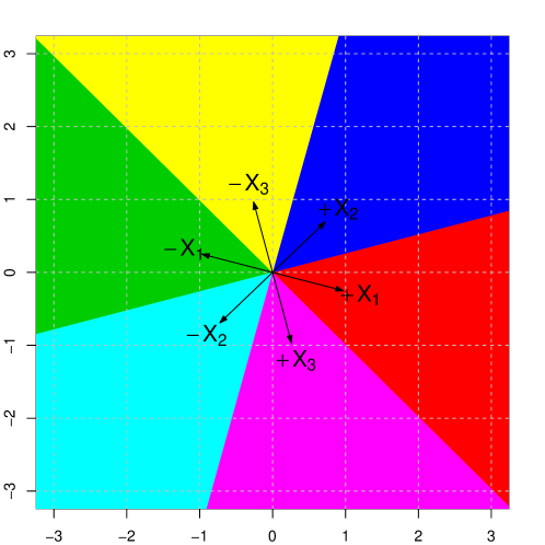
Figure 2: An example of the model selection partition from one step of FS (the variables are normalized, and this is equivalent to one step of LAR, or lasso). Here $n=2$ and $d=3$. The colors indicate the regions of the sample space $\mathbb{R}^{2}$ for which different models—pairs of active variables and signs—are selected, so that, e.g., the red region contains points in $\mathbb{R}^{2}$ that are maximally aligned with $X_{1}$.

For LAR and the lasso, we need to modify the definition of the selected model $\widehat{M}(y)$ in order for the resulting partition elements in (6) to be convex cones. We add an “extra” bit of model information and define $\widehat{M}(y)=\{(\widehat{A}(y),\widehat{s}(y),\widehat{I}_{\ell}(y)):\ell=1,\ldots,k\}$, where $\widehat{I}_{\ell}(y)$ is a list of variables that play a special role in the construction of the LAR or lasso active set at the $\ell$th step, but that a user would not typically pay attention to. In truth, the latter quantity is only a detail that is included so that $\Pi_{M}$, $M\in\pazocal{M}$ are convex cones (without it, the partition elements would each be a union of cones), and so we do not describe it here. Furthermore, it does not affect our treatment of inference in what follows, and for this reason, we will largely ignore the minor differences in model selection events between FS, LAR, and lasso hereafter.

The description of $\widehat{I}_{\ell}(y)$, $\ell=1,\ldots,k$, and the proof that the partition elements $\Pi_{M}$, $M\in\pazocal{M}$ are cones for LAR and lasso, mirrors that in Tibshirani et al. (2016), and is again given in Appendix A.1. Like FS, the active sets from LAR are nested, $\widehat{A}_{1}(y)\subseteq\widehat{A}_{2}(y)\subseteq\widehat{A}_{3}(y)\subseteq\ldots$, since one variable is added to the active set at each step. But for the lasso, this is not necessarily true, as in this case variables can be either added or deleted at each step.

2.2 Inference after selection

We review the selective pivotal inference approach for hypothesis testing after model selection with FS, LAR, or the lasso. The technical details of the TG statistic are deferred to the next two subsections, as they are not needed to understand how the method is used. The null hypotheses we consider are of the form $H_{0}:v^{T}\theta=0$. An important special case occurs when the linear contrast $v^{T}\theta$ gives a normalized coefficient in the regression of $\theta$ onto a subset of the variables in $X$. To be specific, in this case $v=X_{A}(X_{A}^{T}X_{A})^{-1}e_{j}/(e_{j}^{T}(X_{A}^{T}X_{A})^{-1}e_{j})^{1/2}$, for a subset $A\subseteq\{1,\ldots,d\}$, where we let $X_{A}\in\mathbb{R}^{n\times|A|}$ denote the submatrix of $X$ whose columns correspond to elements of $A$ (with $X_{A}^{T}X_{A}$ assumed to be invertible for the chosen subset), and we write $e_{j}$ for the $j$th standard basis vector. This gives

$$v^{T}\theta=\frac{e_{j}^{T}(X_{A}^{T}X_{A})^{-1}X_{A}^{T}\theta}{\sqrt{e_{j}^{T}(X_{A}^{T}X_{A})^{-1}e_{j}}}:=\beta_{j}(A),$$ (7)

and therefore $H_{0}:v^{T}\theta=0$ is a test for the significance of the $j$th normalized coefficient in the linear projection of $\theta$ onto $X_{A}$, written as $\beta_{j}(A)$ for short. (Though the normalization in the denominator is irrelevant for this significance test, it acts as a key scaling factor for the asymptotics in Section 4.) The idea of using a projection parameter for inference, $\beta_{j}(A)$, has also appeared in, e.g., Berk et al. (2013); Wasserman (2014); Lee et al. (2016). Here is now a summary of the testing framework.

• For each possible model $M\in\pazocal{M}$, and any $v\in\mathbb{R}^{n}$ and $\mu\in\mathbb{R}$, a TG statistic $T(\,\cdot\,;M,v,\mu)$ is defined (see (10), in the next subsection), whose domain is the partition element $\Pi_{M}$. This can be used as follows: if $Y$ is drawn from (1), and lands in the partition element $\Pi_{M}$ for model $M$, then the statistic $T(Y;M,v,\mu)$ provides us with a test for the hypothesis $H_{0}:v^{T}\theta=\mu$.

• A concrete case to keep in mind, denoting $M=\{(A_{\ell},s_{\ell}):\ell=1,\ldots,k\}$, is a choice of $v$ such that $v^{T}\theta=\beta_{j}(A_{\ell})$, in the notation of (7). This is the $j$th normalized coefficient in the regression of $\theta$ onto the active variables $X_{A_{\ell}}$, for an active set $A_{\ell}$ at some step $\ell=1,\ldots,k$.

• Assume i.i.d. $N(0,\sigma^{2})$ errors in (1). Under the null hypothesis, the TG statistic has a standard uniform distribution, over draws of $Y$ that land in $\Pi_{M}$. Mathematically, this is the property

  $$\mathbb{P}_{v^{T}\theta=\mu}\Big{(}T(Y;M,v,\mu)\leq t\,\Big{|}\,\widehat{M}(Y)=M\Big{)}=t,$$ (8)

  for all $t\in[0,1]$. The probability above is taken over an arbitrary mean parameter $\theta$ for which $v^{T}\theta=\mu$ (in fact, the TG statistic is constructed so that the law of $T(Y;M,v,\mu)\,|\,\widehat{M}(Y)=M$ only depends on $\theta$ through $v^{T}\theta$, so this is unambiguous). In order for (8) to hold, of course, $v$ and $\mu$ cannot be random, i.e., they cannot depend on $Y$, though they can be functions of $M$.

• Thus $T(Y;M,v,\mu)$ serves as a valid p-value (with exact finite sample size) for testing the null hypothesis $H_{0}:v^{T}\theta=\mu$, conditional on $\widehat{M}(Y)=M$.

• A confidence interval is obtained by inverting the test in (8). Given a desired confidence level $1-\alpha$, we define $C_{\alpha}$ to be the set of all values $\mu$ such that $\alpha/2\leq T(Y;M,v,\mu)\leq 1-\alpha/2$. Then, by construction, the property in (8) (which we reiterate, assumes i.i.d. $N(0,\sigma^{2})$ errors) translates into

  $$\mathbb{P}\Big{(}v^{T}\theta\in C_{\alpha}\,\Big{|}\,\widehat{M}(Y)=M\Big{)}=1-\alpha.$$ (9)

  The interpretation of the above statement is straightforward: the random interval $C_{\alpha}$ contains the fixed parameter $v^{T}\theta$ with probability $1-\alpha$, conditional on $\widehat{M}(Y)=M$.

2.3 The truncated Gaussian pivot

We now describe the truncated Gaussian (TG) pivotal quantity in detail. As defined in Section 2.1, if we write $\widehat{M}(y)$ for the selected model from the given algorithm (FS, LAR, or lasso), run for $k$ steps on $y$, then $\Pi_{M}=\{y:\widehat{M}(y)=M\}$ is a convex cone, for any fixed achieveable model $M$. Hence

$$\Pi_{M}=\{y:\widehat{M}(y)=M\}=\{y:Q_{M}\,y\geq 0\},$$

for a fixed matrix $Q_{M}$ (here the inequality is meant to be interpreted componentwise). Now to define the pivot $T(\,\cdot\,;M,v,\mu)$ for testing $H_{0}:v^{T}\theta=\mu$, several preliminary quantities must be introduced:

$$w=\frac{Q_{M}\,v}{\|v\|_{2}^{2}},\;\;\;a(y;M,v)=v^{T}y-\min_{i:w_{i}>0}\;\frac{(Q_{M}\,y)_{i}}{w_{i}},\;\;\;\text{and}\;\;\;b(y;M,v)=v^{T}y-\max_{i:w_{i}<0}\;\frac{(Q_{M}\,y)_{i}}{w_{i}}.$$

The TG pivot is then defined by

$$T(y;M,v,\mu)=\frac{\displaystyle\Phi\Bigg{(}\frac{b(y;M,v)-\mu}{\sigma\|v\|_{2}}\Bigg{)}-\Phi\Bigg{(}\frac{v^{T}y-\mu}{\sigma\|v\|_{2}}\Bigg{)}}{\displaystyle\Phi\Bigg{(}\frac{b(y;M,v)-\mu}{\sigma\|v\|_{2}}\Bigg{)}-\Phi\Bigg{(}\frac{a(y;M,v)-\mu}{\sigma\|v\|_{2}}\Bigg{)}}.$$ (10)

This has the following property, as stated in (8): when $Y$ is drawn from (1) with i.i.d. $N(0,\sigma^{2})$ errors, and $v^{T}\theta=\mu$, the pivot $T(Y;M,v,\mu)$ is uniformly distributed conditional on $\widehat{M}(Y)=M$. See Lemmas 1 and 2 in Tibshirani et al. (2016) for a proof of this result.

2.4 P-values and confidence intervals

For the null hypothesis $H_{0}:v^{T}\theta=0$, we have seen from (8) that $T(Y;M,v,0)$ acts as a proper (conditional) p-value. But as defined in (10), the statistic $T(Y;M,v,0)$ is implicitly aligned to have power against the one-sided alternative hypothesis $H_{1}:v^{T}\theta>0$. Therefore, when seeking to test the significance of, say, the $j$th coefficient in the projected linear model of $\theta$ on $X_{A_{\ell}}$, we will actually choose $v$ so that

$$v^{T}\theta=(s_{\ell})_{j}\,\beta_{j}(A_{\ell}),$$ (11)

where recall $(s_{\ell})_{j}=\mathrm{sign}(e_{j}^{T}(X_{A_{\ell}}^{T}X_{A_{\ell}})^{-1}X_{A_{\ell}}^{T}y)$ is the sign of the $j$th coefficient in the regression of $y$ onto the set $A_{\ell}$ of active variables, for $y\in\Pi_{M}$. This orients the test in a meaningful direction: $v^{T}\theta>0$ is now the hypothesis that the $j$th coefficient in the projection of $\theta$ onto $X_{A_{\ell}}$ is nonzero, and shares the same sign as the $j$th coefficient in the projection of $y$ onto $X_{A_{\ell}}$, over $y\in\Pi_{M}$; that is, with the above choice of $v$, the p-value $T(Y;M,v,0)$ is designed to be small when the $j$th coefficient in the projection of $Y$ on $X_{A_{\ell}}$ corresponds to a projected population effect that is both large and of the same sign as this computed coefficient. Beyond the current subsection, we will not be explicit about the sign factor in (11) when discussing such contrasts (i.e., those giving regression coefficients in a projected linear model for $\theta$), but it is implicitly understood when computing one-sided p-values.

A statistic aligned to have power against the two-sided alternative $H_{1}:v^{T}\theta\not=0$ is simply given by $2\min\{T(Y;M,v,0),\,1-T(Y;M,v,0)\}$. For purely testing purposes, we find the one-sided p-values discussed above to be more natural, and hence these will serve as our default. On the other hand, for constructing confidence intervals, we prefer to invert the two-sided statistics, since these lead to two-sided intervals. As

$$2\min\{T(Y;M,v,\mu),\;1-T(Y;M,v,\mu)\}\geq\alpha\iff\alpha/2\leq T(Y;M,v,\mu)\leq 1-\alpha/2,$$

the previously described confidence interval in (9) is just given by inverting the two-sided pivot.

To summarize: the default in this work, as with Tibshirani et al. (2016), is to consider one-sided hypothesis tests, but two-sided intervals. These are just two slightly different uses of the same pivot.

2.5 Inference after selection, revisited

We have portrayed selective pivotal inference, in sequential regression procedures, as a method for producing conditional p-values and intervals. An unconditional interpretation of this framework is also possible, which we describe here.

• For each model $M\in\pazocal{M}$, a contrast vector $v_{M}\in\mathbb{R}^{n}$ and pivot value $\mu_{M}\in\mathbb{R}$ are identified, so that the hypothesis $H_{0,M}:v_{M}^{T}\theta=\mu_{M}$ is to be tested whenever $y\in\Pi_{M}$, i.e., whenever $\widehat{M}(y)=M$. A TG statistic $\pazocal{T}(\,\cdot\,;V,U)$ is then defined, whose domain is the entire sample space $\mathbb{R}^{n}$. Here we write $V=\{v_{M}:M\in\pazocal{M}\}$ and $U=\{\mu_{M}:M\in\pazocal{M}\}$ to denote the collection of contrast vectors and pivot values, respectively, across partition elements—we will also refer to these as catalogs. This unconditional TG statistic is defined by

  $$\pazocal{T}(\,\cdot\,;V,U)=\sum_{M\in\pazocal{M}}T(\,\cdot\,;M,v_{M},\mu_{M})\,1_{\Pi_{M}}(\,\cdot\,),$$

  where $1_{\Pi_{M}}(\,\cdot\,)$ denotes the indicator function for the partition element $\Pi_{M}$ (and $T(\,\cdot\,;M,v_{M},\mu_{M})$ is as before, defined in (10)). The unconditional statistic can be used as follows: if a response $Y$ is drawn from (1), then we can form $\pazocal{T}(Y;V,U)=T(Y;\widehat{M}(Y),v_{\widehat{M}(y)},\mu_{\widehat{M}(y)})$ to test the hypothesis $H_{0}:v_{\widehat{M}(Y)}^{T}\theta=\mu_{\widehat{M}(Y)}$.

• A concrete case to keep in mind is when $V$ assigns a contrast vector $v_{M}$ to each model $M$, such that $v_{M}^{T}\theta=\beta_{j_{M}}(A_{\ell_{M}})$, in the notation of (7), where $M=\{(A_{\ell},s_{\ell}):\ell=1,\ldots,k\}$ as usual. This is the $j_{M}$th normalized coefficient from projecting $\theta$ onto $X_{A_{\ell_{M}}}$, the active variables at step $\ell_{M}$.

• Assume that the errors in (1) are i.i.d. $N(0,\sigma^{2})$. Then under the proper hypothesis, by summing up the conditional property in (8) across partition elements, we have

  $$\mathbb{P}_{V^{T}\theta=U}\Big{(}\pazocal{T}(Y;V,U)\leq t\Big{)}=t,$$ (12)

  for all $t\in[0,1]$. The assertion above holds for a parameter $\theta$ such that $V^{T}\theta=U$, which we use as shorthand for $v_{M}^{T}\theta=\mu_{M}$ for all $M\in\pazocal{M}$. Note that this full specification, across all $M\in\pazocal{M}$, is critical in order to apply the relevant null probability within each partition element (giving rise to the equality in (12)).

• Therefore $\pazocal{T}(Y;V,U)$ serves as a valid p-value (with exact finite sample size)—but for testing what null hypothesis? Formally, it is attached to $H_{0}:V^{T}\theta=U$, an exhaustive specification of $v_{M}^{T}\theta=\mu_{M}$, over all $M\in\pazocal{M}$, but in truth, $\pazocal{T}(Y;V,U)$ carries no information about models other than the selected one, $\widehat{M}(Y)$. For this reason, we actually consider $\pazocal{T}(Y;V,U)$ to be a p-value for the random null hypothesis $H_{0}:v_{\widehat{M}(Y)}^{T}\theta=\mu_{\widehat{M}(Y)}$. This is made more precise through confidence intervals.

• A confidence interval is obtained by inverting the test in (12). But the TG statistic at $Y$,

  $$\pazocal{T}(Y;V,U)=\sum_{M\in\pazocal{M}}T(Y;M,v_{M},\mu_{M})1_{\Pi_{M}}(Y)=T\big{(}Y;\widehat{M}(Y),v_{\widehat{M}(Y)},\mu_{\widehat{M}(Y)}\big{)},$$

  only depends on $U$ through $\mu_{\widehat{M}(Y)}$. Thus, given a desired confidence level $1-\alpha$, let us define $D_{\alpha}$ to be the set of $U$ such that $\alpha/2\leq\pazocal{T}(Y;V,U)\leq 1-\alpha/2$, and $C_{\alpha}$ to be the set of $\mu_{\widehat{M}(Y)}$ such that $\alpha/2\leq T(Y;\widehat{M}(Y),v_{\widehat{M}(Y)},\mu_{\widehat{M}(Y)})\leq 1-\alpha/2$. Then we can see that

  $$U\in D_{\alpha}\iff\mu_{\widehat{M}(Y)}\in C_{\alpha},$$

  so the confidence interval is effectively infinite with respect to the values $\mu_{M}$, $M\not=\widehat{M}(Y)$, and inverting the test in (12) yields

  $$\mathbb{P}\Big{(}v_{\widehat{M}(Y)}^{T}\theta\in C_{\alpha}\Big{)}=1-\alpha.$$ (13)

  The above expression says that the random interval $C_{\alpha}$ traps the random parameter $v_{\widehat{M}(Y)}^{T}\theta$ with probability $1-\alpha$, and thus, this supports the interpretation of $H_{0}:v_{\widehat{M}(Y)}^{T}\theta=\mu_{\widehat{M}(Y)}$ as the null hypothesis underlying the unconditional TG statistic.

Remark 1.

The pivotal property in (12) is derived under the distributional assumption that $V^{T}\theta=U$, i.e., $v_{M}^{T}\theta=\mu_{M}$ for all $M\in\pazocal{M}$, which may seem unnatural, as the catalog $U$ of pivot value can be large (e.g., on the order of $d^{k}$ after $k$ steps of FS), and so this is condition on possibly many contrasts of $\theta$. However, it is worth emphasizing that the unconditional testing property in (12) is really only useful in that it allows us to formulate the unconditional confidence interval property in (13), which is a more natural statement about coverage of a single (random) parameter. When viewing selective inference from an unconditional perpsective, we find it more natural to place the focus on confidence intervals rather than hypothesis testing; in many ways, we find the former the more natural of the two perspectives, unconditionally. Tibshirani et al. (2016) in fact suggest separate nomenclature for the unconditional case, referring to the property in (13) as that of a selection interval (rather than confidence interval), to emphasize that this interval covers a moving target.

3 The master statistic

Given a response $y$ and predictors $X$, our description thus far of the selected model $\widehat{M}(y)$, statistics $T(y;M,v,\mu)$ and $\pazocal{T}(y;V,U)$, etc., has ignored the role of $X$. This was done for simplicity. The theory to come in Section 4 will consider $X$ to be nonrandom, but asymptotically $X$ must (of course) grow with $n$, and so it will help to be precise about the dependence of the selected model and statistics on $X$. We will denote these quantities by $\widehat{M}(X,y)$, $T(X,y;M,v,\mu)$, and $\pazocal{T}(X,y;V,U)$ to emphasize this dependence. We define

$$\Omega_{n}=\Big{(}\frac{1}{n}X^{T}X,\frac{1}{\sqrt{n}}X^{T}y\Big{)},$$

a $d(d+3)/2$-dimensional quantity that we will call the master statistic. As its name might suggest, this plays an important role: all normalized coefficients from regressing $y$ onto subsets of the variables $X$ can be written in terms of $\Omega_{n}$. That is, for an arbitrary set $A\subseteq\{1,\ldots,p\}$, the $j$th normalized coefficient from the regression of $y$ onto $X_{A}$ is

$$\frac{(e_{j}^{T}X_{A}^{T}X_{A})^{-1}X_{A}^{T}y}{\sqrt{e_{j}^{T}(X_{A}^{T}X_{A})^{-1}e_{j}}}=\frac{e_{j}^{T}n(X_{A}^{T}X_{A})^{-1}\frac{1}{\sqrt{n}}X_{A}^{T}y}{\sqrt{e_{j}^{T}n(X_{A}^{T}X_{A})^{-1}e_{j}}},$$

which only depends on $(X,y)$ through $\Omega_{n}$. The same dependence is true, it turns out, for the selected models from FS, LAR, and the lasso. We defer the proof of the next lemma, as with all proofs in this paper, until the appendix.

Lemma 3.

For each of the FS, LAR, and lasso procedures, run for $k$ steps on data $(X,y)$, the selected model $\widehat{M}(X,y)$ only depends on $(X,y)$ through $\Omega_{n}=(\frac{1}{n}X^{T}X,\frac{1}{\sqrt{n}}X^{T}y)$, the master statistic.

In more detail, for any fixed $M\in\pazocal{M}$, the matrix $Q_{M}(X)$ such that $\widehat{M}(X,y)=M\iff Q_{M}(X)\,y\geq 0$ can be written as $Q_{M}(X)=P_{M}(\frac{1}{n}X^{T}X)\,\frac{1}{\sqrt{n}}X^{T}$, where $P_{M}$ depends only on $\frac{1}{n}X^{T}X$. Hence

$$\widehat{M}(X,y)=M\iff P_{M}\Big{(}\frac{1}{n}X^{T}X\Big{)}\,\frac{1}{\sqrt{n}}X^{T}y\geq 0.$$

This lemma asserts that the master statistic governs model selection, as performed by FS, LAR, and the lasso. It is also central to TG pivot for these procedures. Denoting $M=\widehat{M}(X,y)$, the statistic $T(X,y;M,v,\mu)$ in (10) only depends on $(X,y)$ through three quantities:

$$\frac{v^{T}y}{\|v\|_{2}},\;\;\;\frac{Q_{M}(X)\,v}{\|v\|_{2}},\;\;\;\text{and}\;\;\;Q_{M}(X)\,y.$$

The third quantity is always a function of $\Omega_{n}$, by Lemma 3. When $v$ is chosen so that $v^{T}y$ is a normalized coefficient in the regression of $y$ onto a subset of the variables in $X$, the first two quantities are also functions of $\Omega_{n}$. Thus, in this case, the TG pivot only depends on $(X,y)$ through the master statistic $\Omega_{n}$; in fact, it is continuous at any point such that $\frac{1}{n}X^{T}X$ is nonsingular and $y$ does not lie on the boundary of a model selection event.

Lemma 4.

Fix any model $M\in\pazocal{M}$, and suppose that $v$ is chosen so that $v^{T}y$ is a normalized coefficient from projecting $y$ onto a subset of the variables in $X$. Then the TG statistic only depends on $(X,y)$ by means of $\Omega_{n}$, so that we may write

$$T(X,y;M,v,\mu)=\psi_{M}\Big{(}\frac{1}{n}X^{T}X,\frac{1}{\sqrt{n}}X^{T}y\Big{)}.$$

Further, the function $\psi_{M}$ is continous at any point $(S,z)$ such that $S$ is nonsingular and $P_{M}(S)\,z>0$.

Finally, we show that the conditional pivotal property of the TG statistic in (8) can be phrased entirely in terms of the master statistic.

Lemma 5.

Assume the conditions of Lemma 4, and additionally that $Y$ is drawn from (1). Construct the master statistic $\Omega_{n}=(\frac{1}{n}X^{T}X,\frac{1}{\sqrt{n}}X^{T}Y)$. Then there is a function $g$ such that

$$v^{T}\theta=g(\mathbb{E}(\Omega_{n})).$$

Thus if the errors in (1) are i.i.d. $N(0,\sigma^{2})$, then the conditional pivotal property (8) of the TG statistic can be reexpressed as

$$\mathbb{P}_{g(\mathbb{E}(\Omega_{n}))=\mu}\Big{(}\psi_{M}(\Omega_{n})\leq t\,\Big{|}\,\widehat{M}(X,Y)=M\Big{)}=t,$$

for all $t\in[0,1]$.

Equipped with the last two lemmas, asymptotic theory for the TG test, when $d$ is fixed, is not far off. Under weak conditions on the data model in (1), the central limit theorem tells us that $\frac{1}{\sqrt{n}}X^{T}Y$ converges weakly to a normal random variable. With $\frac{1}{n}X^{T}X$ converging to a deterministic matrix, the continuous mapping theorem will then provide the appropriate asymptotic limit for the statistic $T(X,y;M,v,\mu)=\psi_{M}(\frac{1}{n}X^{T}X,\frac{1}{\sqrt{n}}X^{T}Y)$. This is made more precise next.

4 Asymptotic theory

Here we treat the dimension $d$ as fixed, and consider the limiting distribution of the TG statistic as $n\to\infty$. (See Section 7 for the case when $d$ grows.) Throughout, the matrix $X\in\mathbb{R}^{n\times d}$ will be treated as nonrandom, and we consider a sequence of predictor matrices satisfying two conditions:

$$\lim_{n\to\infty}\;\frac{1}{n}X^{T}X=\Sigma,$$ (14)

for a nonsingular matrix $\Sigma\in\mathbb{R}^{d\times d}$, and

$$\lim_{n\to\infty}\;\max_{i=1,\ldots,n}\;\frac{\|x_{i}\|_{2}}{\sqrt{n}}=0,$$ (15)

where $x_{i}\in\mathbb{R}^{d}$, $i=1,\ldots,n$ denote the rows of $X$. These are not strong conditions.

4.1 A nonparametric family of distributions

We specify the class of distributions that we will be working with for $Y$ in (1). Let $\sigma^{2}>0$ be a fixed, known constant. First we define a set of error distributions

$$\pazocal{E}=\Bigg{\{}F\;:\;\int xdF(x)=0,\;\int x^{2}dF(x)=\sigma^{2}\Bigg{\}}.$$

The first moment condition in the above definition is needed to make the model identifiable, and the second condition is used for simplicity. Aside from these moment conditions, the class $\pazocal{E}$ contains a small neighborhood (say, as measured in the total variation metric) around essentially every element. Thus, modulo the moment assumptions, $\pazocal{E}$ is strongly nonparametric in the sense of Donoho (1988). Given $\mu\in\mathbb{R}$, let $F_{\mu}$ denote the distribution of $\mu+\delta$, where $\delta\sim F$, and given $\theta=(\theta_{1},\ldots,\theta_{n})\in\mathbb{R}^{n}$, let $F_{n}(\theta)=F_{\theta_{1}}\times\ldots,\times F_{\theta_{n}}$. Now we define a class of distributions

$$\pazocal{P}_{n}(\theta)=\Bigg{\{}F_{n}(\theta)=F_{\theta_{1}}\times\ldots\times F_{\theta_{n}}\;:\;F\in\pazocal{E}\Bigg{\}}.$$ (16)

In words, assigning a distribution $Y\sim F_{n}(\theta)$ means that $Y$ in drawn from the model (1), with mean $\theta\in\mathbb{R}^{n}$, and errors $\epsilon_{1},\ldots,\epsilon_{n}$ i.i.d. from an arbitrary centered distribution $F$ with variance $\sigma^{2}$.

As $n$ grows, we allow the underlying mean $\theta$ to change, but we place a restriction on this parameter so that it has an appropriate asymptotic limit. Specifically, we consider a class $\Theta$ of sequences of mean parameters such that $\frac{1}{\sqrt{n}}X^{T}\theta$ has an asymptotic limit lying in some compact set, with uniform convergence to this limit. Formally, write (in a slight abuse of notation) $\theta\in\Theta$ to denote a sequence of mean parameters in $\Theta$, and let $E(\Theta)$ denote the set of limit points of $\{\frac{1}{\sqrt{n}}X^{T}\theta:\theta\in\Theta\}$. Then, for some constant $B>0$, we require of the class $\Theta$,

$$E(\Theta)\subseteq[-B,B]^{d},\;\;\;\text{and}\;\;\;\lim_{n\to\infty}\;\sup_{\eta\in E(\Theta)}\;\sup_{\frac{1}{\sqrt{n}}X^{T}\theta\to\eta}\;\Bigg{|}\frac{1}{\sqrt{n}}X^{T}\theta-\eta\Bigg{|}=0.$$ (17)

We emphasize once again that $\theta\in\mathbb{R}^{n}$ and $X\in\mathbb{R}^{n\times p}$ will both vary with $n$, i.e., we can think of $\theta$ and the columns of $X$ as triangular arrays, but our notation suppresses this dependence for simplicity.

4.2 Uniform convergence results

We begin with a result on the uniform convergence of (the random part of) the master statistic to a normal distribution, both marginally and conditionally.

Lemma 6.

Assume that $X$ has asymptotic covariance matrix $\Sigma$, as in (14), and satisfies the normalization condition in (15). Let $Y\sim F_{n}(\theta)\in\pazocal{P}_{n}(\theta)$, this class as defined in (16), for a sequence of mean parameters $\theta\in\Theta$, as defined in (17). Denote $\frac{1}{\sqrt{n}}X^{T}\theta\to\eta$ as $n\to\infty$. Then $Z_{n}=\frac{1}{\sqrt{n}}X^{T}Y$ converges in distribution to $Z\sim N(\eta,\sigma^{2}\Sigma)$, uniformly over $\pazocal{P}_{n}(\theta)$, and uniformly over all $\theta\in\Theta$. That is,

$$\lim_{n\to\infty}\;\sup_{\theta\in\Theta}\;\sup_{F_{n}(\theta)\in\pazocal{P}_{n}(\theta)}\;\sup_{x\in\mathbb{R}^{d}}\;\big{|}\mathbb{P}(Z_{n}\leq x)-\mathbb{P}(Z\leq x)\big{|}=0.$$

Further, given a sequence of matrices $A_{n}\in\mathbb{R}^{q\times d}$, $n=1,2,3,\ldots$ with $A_{n}\to A$ as $n\to\infty$, such that the set $\{z:Az\geq 0\}$ has nonempty interior, $Z_{n}\,|\,A_{n}Z_{n}\geq 0$ converges in distribution to $Z\,|\,AZ\geq 0$, uniformly over $\pazocal{P}_{n}(\theta)$, and uniformly over all $\theta\in\Theta$.

This lemma, combined with Lemmas 4 and 5 of the last section, leads us to uniform asymptotic theory for the TG test. We remind the reader that $k$, the number of steps, is to be considered fixed in the next result (as it is throughout the paper).

Theorem 7.

Assume the conditions of Lemma 6. Suppose FS, LAR, or the lasso is run for $k$ steps on $(X,Y)$. Below we describe the conditional and unconditional asymptotic results separately.

(a, Markovic) Fix any model $M\in\pazocal{M}$. Let $v$ be a vector such that $v^{T}\theta$ gives a normalized coefficient in the projection of $\theta$ onto some subset of the variables in $X$, and let $\mu$ be an arbitrary pivot value. Then under $v^{T}\theta=\mu$, the conditional TG statistic $T(X,Y;M,v,\mu)\,|\,\widehat{M}(X,Y)=M$ converges in distribution to $W\sim U(0,1)$, uniformly over $\pazocal{P}_{n}(\theta)$, and over $\theta\in\Theta$. That is,

$$\lim_{n\to\infty}\;\sup_{\theta\in\Theta}\;\sup_{F_{n}(\theta)\in\pazocal{P}_{n}(\theta)}\;\sup_{t\in[0,1]}\;\Bigg{|}\mathbb{P}_{v^{T}\theta=\mu}\Big{(}T(X,Y;M,v,\mu)\leq t\,\Big{|}\,\widehat{M}(X,Y)=M\Big{)}-t\Bigg{|}=0.$$

Moreover, if we define $C_{n,\alpha}$ to be the set of $\mu$ such that $\alpha/2\leq T(X,Y;M,v,\mu)\leq 1-\alpha/2$, then $C_{n,\alpha}$ is an asymptotically uniformly valid confidence interval for $v^{T}\theta$. That is,

$$\lim_{n\to\infty}\;\sup_{\theta\in\Theta}\;\sup_{F_{n}(\theta)\in\pazocal{P}_{n}(\theta)}\;\sup_{\alpha\in[0,1]}\;\Bigg{|}\mathbb{P}_{v^{T}\theta=\mu}\Big{(}v^{T}\theta\in C_{n,\alpha}\,\Big{|}\,\widehat{M}(X,Y)=M\Big{)}-(1-\alpha)\Bigg{|}=0.$$

(b) Let $V=\{v_{M}:M\in\pazocal{M}\}$ be a catalog of vectors such that each $v_{M}^{T}\theta$ yields a normalized coefficient in the projection of $\theta$ onto a subset of the variables in $X$, for $M\in\pazocal{M}$, and $U=\{\mu_{M}:M\in\pazocal{M}\}$ be a catalog of pivot values. Then under $V^{T}\theta=U$, the same results as in part (a) hold marginally. That is,

$$\lim_{n\to\infty}\;\sup_{\theta\in\Theta}\;\sup_{F_{n}(\theta)\in\pazocal{P}_{n}(\theta)}\;\sup_{t\in[0,1]}\;\Big{|}\mathbb{P}_{V^{T}\theta=U}\Big{(}\pazocal{T}(X,Y;V,U)\leq t\Big{)}-t\Big{|}=0.$$

and for $C_{n,\alpha}$ defined to be the set of $\mu$ such that $\alpha/2\leq T(X,Y;\widehat{M}(X,Y),v_{\widehat{M}(X,Y)},\mu)\leq 1-\alpha/2$,

$$\lim_{n\to\infty}\;\sup_{\theta\in\Theta}\;\sup_{F_{n}(\theta)\in\pazocal{P}_{n}(\theta)}\;\sup_{\alpha\in[0,1]}\;\Big{|}\mathbb{P}\Big{(}v_{\widehat{M}(X,Y)}^{T}\theta\in C_{n,\alpha}\Big{)}-(1-\alpha)\Big{|}=0.$$

Remark 2.

An initial version of this work contained only the unconditional result in part (b) of the theorem. Jelena Markovic pointed out that the conditional result in part (a) should also be possible, and thus this conditional result should also be attributed to her. Between the initial and the current version of this paper, in addition to revising Theorem 7, we have also revised Theorems 11 and 12 to include the appropriate conditional results.

5 Unknown $\sigma^{2}$ and the bootstrap

The results of the previous section assumed that the error variance $\sigma^{2}$ in the model (1) was known. Here we consider two strategies when $\sigma^{2}$ is unknown. The first plugs a (rather naive) estimate of $\sigma^{2}$ into the usual TG statistic. The second is a computationally efficient bootstrap method. Both, as we will show, yield asymptotically conservative p-values. (In practice, the bootstrap often gives shorter confidence intervals than those based on the TG pivot; see Section 6.)

5.1 A simple plug-in approach

Given a model $M\in\pazocal{M}$, contrast vector $v$, and pivot value $\mu$, consider the TG statistic $T(X,Y;M,v,\mu)$. Let us abbreviate

$$\widehat{a}_{M}=a(X,Y;M,v),\;\;\;\text{and}\;\;\;\widehat{b}_{M}=b(X,Y;M,v),$$

where the latter two functions are as defined in Section 2.3. In this notation, we can succintly write the TG statistic as

$$T(X,Y;M,v,\mu)=\frac{\displaystyle\Phi\Bigg{(}\frac{\widehat{b}_{M}-\mu}{\sigma\|v\|_{2}}\Bigg{)}-\Phi\Bigg{(}\frac{v^{T}Y-\mu}{\sigma\|v\|_{2}}\Bigg{)}}{\displaystyle\Phi\Bigg{(}\frac{\widehat{b}_{M}-\mu}{\sigma\|v\|_{2}}\Bigg{)}-\Phi\Bigg{(}\frac{\widehat{a}_{M}-\mu}{\sigma\|v\|_{2}}\Bigg{)}}.$$ (18)

When $\sigma^{2}$ is unknown, we propose a simple plug-in approach that replaces $\sigma$ with $cs_{Y}$, where

$$s_{Y}^{2}=\frac{1}{n}\sum_{i=1}^{n}|Y_{i}-\overline{Y}|^{2},$$

the sample variance of $Y$ (here $\overline{Y}=\sum_{i=1}^{n}Y_{i}/n$ denotes the sample mean), and $c>1$ is a fixed constant. To be explicit, we consider the modified TG statistic

$$\widetilde{T}(X,Y;M,v,\mu)=\frac{\displaystyle\Phi\Bigg{(}\frac{\widehat{b}_{M}-\mu}{cs_{Y}\|v\|_{2}}\Bigg{)}-\Phi\Bigg{(}\frac{v^{T}Y-\mu}{cs_{Y}\|v\|_{2}}\Bigg{)}}{\displaystyle\Phi\Bigg{(}\frac{\widehat{b}_{M}-\mu}{cs_{Y}\|v\|_{2}}\Bigg{)}-\Phi\Bigg{(}\frac{\widehat{a}_{M}-\mu}{cs_{Y}\|v\|_{2}}\Bigg{)}}.$$ (19)

The scaling factor $c$ facilitates our theoretical study of the above plug-in statistic, and practically, we have found that ignoring it (i.e., setting $c=1$) works perfectly well, though a choice of, say, $c=1.0001$ seems to have a minor effect anyway.

When the mean $\theta$ of $Y$ is nonzero, the sample variance $s_{Y}^{2}$ is generally too large as an estimate of $\sigma^{2}$. As we will show, the modified statistic in (19) thus yields asymptotically conservative p-values. Residual based estimates of $\sigma^{2}$ are not as useful in our setting because they depend more heavily on the linearity of the underlying regression model, and they suffer practically when $d$ is close to $n$ (see also the discussion at the start of Section 6).

5.2 An efficient bootstrap approach

As an alternative to the plug-in method of the last subsection, we investigate a highly efficient bootstrap scheme that does not rely on knowledge of $\sigma^{2}$. Our general framework so far treats $X$ as fixed, and for our bootstrap strategy to respect this assumption, we cannot use, say, the pairs bootstrap, and must perform sampling with respect to $Y$ only. The residual bootstrap is ruled out since we do not assume that the mean $\theta$ follows a linear model in $X$. This leaves us to consider simple bootstrap sampling of the components of $Y$. This is somewhat nonstandard, as the components of $Y$ in (1) are not i.i.d., but it provides a mechanism for provably conservative asymptotic inference, and it is what makes our approach so computationally efficient.

Given $Y=(Y_{1},\ldots,Y_{n})$ drawn from the model in (1), let $Y^{*}=(Y_{1}^{*},\ldots,Y_{n}^{*})$ denote a bootstrap sample of $Y$. We will denote by $\mathbb{P}_{*}$ the conditional distribution of $Y^{*}$ on $Y$, and $\mathbb{E}_{*}$ the associated expectation operator. That is, $\mathbb{P}_{*}(Y^{*}\in A)$ is shorthand for $\mathbb{P}(Y^{*}\in A|Y)$, and similarly for $\mathbb{E}_{*}$. Using the notation of the last subsection (notation for $\widehat{a}_{M},\widehat{b}_{M}$), and assuming without a loss of generality that $\|v\|_{2}=1$, let us motivate our bootstrap proposal by expressing the TG statistic as

$$T(X,Y;M,v,\mu)=\mathbb{P}\Big{(}Z_{\mu,\sigma^{2}}\geq v^{T}Y\,\Big{|}\,\widehat{a}_{M}\leq Z_{\mu,\sigma^{2}}\leq\widehat{b}_{M},\,Y\Big{)},$$

where the probability on the right-hand side is taken with $Y$ (and thus $\widehat{a}_{M},\widehat{b}_{M}$) treated as fixed, and with $Z_{\mu,\sigma^{2}}$ denoting a $N(\mu,\sigma^{2})$ random variable. The main idea is now to approximate the truncated normal distribution underlying the TG statistic with an appropriate one from bootstrap samples,

$$\mathbb{P}\Big{(}Z_{\mu,\sigma^{2}}\geq v^{T}Y\,\Big{|}\,\widehat{a}_{M}\leq Z_{\mu,\sigma^{2}}\leq\widehat{b}_{M},\,Y\Big{)}\approx\mathbb{P}_{*}\Big{(}v^{T}(Y^{*}-\overline{Y}\mathbb{1})+\mu\geq v^{T}Y\,\Big{|}\,\widehat{a}_{M}\leq v^{T}(Y^{*}-\overline{Y}\mathbb{1})+\mu\leq\widehat{b}_{M}\Big{)}.$$

Recall $\overline{Y}=\sum_{i=1}^{n}Y_{i}/n$ is the sample mean of $Y$, so $\mathbb{E}_{*}(v^{T}Y^{*})=v^{T}(\overline{Y}\mathbb{1})$ (with $\mathbb{1}\in\mathbb{R}^{n}$ denoting the vector of all 1s), and we have shifted $v^{T}Y^{*}$ so that the resulting quantity $v^{T}(Y^{*}-\overline{Y}\mathbb{1})+\mu$ mimics a normal variable with mean $\mu$. The right-hand side above very nearly defines our bootstrap version of the TG statistic, except that for technical reasons, we must make two small modifications. In particular, we define the bootstrap TG statistic as

$$T^{*}(X,Y;M,v,\mu)=\frac{\mathbb{P}_{*}\big{(}v^{T}Y\leq cv^{T}(Y^{*}-\overline{Y}\mathbb{1})+\mu\leq\widehat{b}_{M}\big{)}+\delta_{n}}{\mathbb{P}_{*}\big{(}\widehat{a}_{M}\leq cv^{T}(Y^{*}-\overline{Y}\mathbb{1})+\mu\leq\widehat{b}_{M}\big{)}+\delta_{n}},$$ (20)

where $c>1$ is a constant as before, and $\delta_{n}=\gamma n^{-1/4}$ for a small constant $\gamma>0$. Again, we have found that ignoring the scaling factor $c$ (i.e., setting $c=1$) works just fine in practice, though a choice like $c=1.0001$ does not cause major differences anyway. On the contrary, a nonzero choice of the padding factor like $\delta_{n}=10^{-4}n^{-1/4}$ does play an important practical role, since the bootstrap probabilities in the numerator and denominator in (20) can sometimes be zero.

Lastly, it is worth emphasizing that practical estimation of the bootstrap probabilities appearing in (20) is quite an easy computational task, because the regression procedure in question, be it FS, LAR, or the lasso, need not be rerun beyond its initial run on the observed $Y$. After this initial run, we can just save the realized quantities $\widehat{a}_{M},\widehat{b}_{M}$, and then draw, say, $B=1000$ bootstrap samples $Y^{*}$ in order to estimate the probabilities in (20). This is not at all computationally expensive. Moreover, to estimate (20) over multiple trial values of $\mu$ (so that we can invert these bootstrap p-values for a bootstrap confidence interval), only a single common set of bootstrap samples is needed, since we can just shift $v^{T}Y^{*}$ appropriately for each bootstrap sample $Y^{*}$.

5.3 Asymptotic theory for unknown $\sigma^{2}$

Treating the dimension $d$ as fixed, we will assume the previous limiting conditions (14), (15) on the matrix $X$, and additionally, that

$$\frac{1}{n}\sum_{i=1}^{n}\|x_{i}\|_{2}^{3}=O(1).$$ (21)

Note that (14) already implies that $\frac{1}{n}\sum_{i=1}^{n}\|x_{i}\|_{2}^{2}\to\mathrm{tr}(\Sigma)$, and the above is a little stronger, though it is still not a strong condition by any means. For example, it is satisfied when $\max_{i=1,\ldots,n}\|x_{i}\|_{2}=O(1)$. These conditions on $X$ imply important scaling properties for our usual choices of contrast vectors.

Lemma 8.

Assume that $X$ satisfies (14), (15), (21). If $v$ is any vector such that $v^{T}\theta$ gives a normalized regression coefficient from projecting $\theta$ onto some subset of the variables in $X$, then

$$\|v\|_{3}^{3}=O\Big{(}\frac{1}{\sqrt{n}}\Big{)}.$$

We specify assumptions on the distribution of $Y$ in (1) that are similar to (but slightly stronger than) those in Section 4.1. For constants $\sigma^{2},\tau,\kappa>0$, we define a set of error distributions

$$\pazocal{E}^{\prime}=\Bigg{\{}F\;:\;\int xdF(x)=0,\;\int x^{2}dF(x)=\sigma^{2},\;\int x^{3}dF(x)\leq\tau,\;\int x^{4}dF(x)\leq\kappa\Bigg{\}}.$$

We also define a class of distributions

$$\pazocal{P}^{\prime}_{n}(\theta)=\Bigg{\{}F_{n}(\theta)=F_{\theta_{1}}\times\ldots\times F_{\theta_{n}}\;:\;F\in\pazocal{E}^{\prime}\Bigg{\}}.$$ (22)

where as before, $F_{\mu}$ denotes the distribution of $\mu+\delta$, for $\delta\sim F$. We define a class $\Theta^{\prime}$ of sequences of mean parameters that satisfies, as before,

$$E(\Theta^{\prime})\subseteq[-B,B]^{d},\;\;\;\text{and}\;\;\;\lim_{n\to\infty}\;\sup_{\eta\in E(\Theta^{\prime})}\;\sup_{\frac{1}{\sqrt{n}}X^{T}\theta\to\eta}\;\Bigg{|}\frac{1}{\sqrt{n}}X^{T}\theta-\eta\Bigg{|}=0,$$ (23)

for a constant $B>0$, where recall $E(\Theta^{\prime})$ denotes the set of limit points in $\Theta^{\prime}$; also, for each $\theta\in\Theta^{\prime}$, at each $n$, we require

$$s_{\theta}^{2}=\frac{1}{n}\sum_{i=1}^{n}|\theta_{i}-\overline{\theta}|^{2}\leq S,\;\;\;\text{and}\;\;\;r_{\theta}^{3}=\frac{1}{n}\sum_{i=1}^{n}|\theta_{i}-\overline{\theta}|^{3},$$ (24)

for constants $S,R>0$, where $\overline{\theta}=\sum_{i=1}^{n}\theta_{i}/n$. Note that the assumptions $Y\sim F_{n}(\theta)$, with $F_{n}(\theta)\in\pazocal{P}^{\prime}_{n}(\theta)$ and $\theta\in\Theta^{\prime}$, are not much stronger than our assumptions in Section 4.1: we require the existence of two more moments for the error distribution, and place an additional weak condition on the growth of (components of) $\theta$. These conditions are sufficient to prove the following helpful lemma.

Lemma 9.

Assume that $X$ satisfies (14), (15). Let $Y\sim F_{n}(\theta)\in\pazocal{P}^{\prime}_{n}(\theta)$, where this class is as defined in (22), and let $\theta\in\Theta^{\prime}$, where this class is as in (23), (24). Then for any fixed $M\in\pazocal{M}$, and $c>1$,

$$\lim_{n\to\infty}\;\sup_{\theta\in\Theta^{\prime}}\;\sup_{F_{n}(\theta)\in\pazocal{P}^{\prime}_{n}(\theta)}\;\mathbb{P}\Big{(}cs_{Y}\geq\sigma\,\Big{|}\,\widehat{M}(X,Y)=M\Big{)}=1.$$

In words, the event $\{cs_{Y}\geq\sigma\}$ has probability tending to 1 conditional on $\widehat{M}(X,Y)=M$, uniformly over $\pazocal{P}^{\prime}_{n}(\theta)$, and over $\theta\in\Theta^{\prime}$. Furthermore, denoting the sample third moment of $Y$ as

$$r_{Y}^{3}=\frac{1}{n}\sum_{i=1}^{n}|Y_{i}-\overline{Y}|^{3},$$

we have that for any $\delta>0$, there exists $C>0$ such that for sufficiently large $n$,

$$\sup_{\theta\in\Theta^{\prime}}\;\sup_{F_{n}(\theta)\in\pazocal{P}^{\prime}_{n}(\theta)}\;\mathbb{P}\Bigg{(}\frac{r_{Y}^{3}}{s_{Y}^{3}}\geq C\,\Bigg{|}\,\widehat{M}(X,Y)=M\Bigg{)}\leq\delta,$$

In words, $r_{Y}^{3}/s_{Y}^{3}=O_{\mathbb{P}}(1)$ conditional on $\widehat{M}(X,Y)=M$, uniformly over $\pazocal{P}^{\prime}_{n}(\theta)$, and over $\theta\in\Theta^{\prime}$.

The last two lemmas allow us to tie the distribution function of our bootstrap contrast to that of a normal random variable.

Lemma 10.

Assume that $X$ satisfies (14), (15), (21). Let $Y\sim F_{n}(\theta)\in\pazocal{P}^{\prime}_{n}(\theta)$, as defined in (22), and let $\theta\in\Theta^{\prime}$, as defined in (23), (24). Let $M\in\pazocal{M}$, and let $v$ be such that $v^{T}\theta$ gives a normalized regression coefficient from projecting $\theta$ onto a subset of the variables in $X$. Then for any $\delta>0$, there exists $C>0$ such that sufficiently large $n$,

$$\sup_{\theta\in\Theta^{\prime}}\;\sup_{F_{n}(\theta)\in\pazocal{P}^{\prime}_{n}(\theta)}\;\mathbb{P}\Bigg{(}\sup_{t\in\mathbb{R}}\;\big{|}\mathbb{P}_{*}\big{(}v^{T}(Y^{*}-\overline{Y}\mathbb{1})\leq t\big{)}-\mathbb{P}\big{(}s_{Y}Z\leq t\,\big{|}\,Y\big{)}\big{|}\geq\frac{C}{\sqrt{n}}\,\Bigg{|}\,\widehat{M}(X,Y)=M\Bigg{)}\leq\delta,$$

where we use $Z\sim N(0,1)$ for a standard normal random variate. In words, $\sup_{t\in\mathbb{R}}|\mathbb{P}_{*}(v^{T}(Y^{*}-\overline{Y}\mathbb{1})\leq t)-{}$ $\mathbb{P}(s_{Y}Z\leq t\,|\,Y)|=O_{\mathbb{P}}(1/\sqrt{n})$ conditional on $\widehat{M}(X,Y)=M$, uniformly over $\pazocal{P}^{\prime}_{n}(\theta)$, and over $\theta\in\Theta^{\prime}$.

We are now ready to present uniform asymptotic results for the plug-in and bootstrap TG statistics. We remind the reader the number of steps $k$ is treated as fixed below (as it is throughout).

Theorem 11.

Assume the conditions of Lemma 10. Suppose FS, LAR, or the lasso is run for $k$ steps on $(X,Y)$. Then under $v^{T}\theta=0$, the conditional plug-in TG statistic $\widetilde{T}(X,Y;M,v,0)\,|\,\widehat{M}(X,Y)=M$ and conditional bootstrap TG statistic $T^{*}(X,Y;M,v,0)\,|\,\widehat{M}(X,Y)=M$ are each asymptotically larger than $U(0,1)$ in distribution, uniformly over $\pazocal{P}^{\prime}_{n}(\theta)$, and over $\theta\in\Theta^{\prime}$. That is,

$$\lim_{n\to\infty}\;\sup_{\theta\in\Theta^{\prime}}\;\sup_{F_{n}(\theta)\in\pazocal{P}^{\prime}_{n}(\theta)}\;\sup_{t\in[0,1]}\;\Big{[}\mathbb{P}_{v^{T}\theta=0}\Big{(}\widetilde{T}(X,Y;M,v,0)\leq t\,\Big{|}\,\widehat{M}(X,Y)=M\Big{)}-t\Big{]}_{+}=0,$$

and

$$\lim_{n\to\infty}\;\sup_{\theta\in\Theta^{\prime}}\;\sup_{F_{n}(\theta)\in\pazocal{P}^{\prime}_{n}(\theta)}\;\sup_{t\in[0,1]}\;\Big{[}\mathbb{P}_{v^{T}\theta=0}\Big{(}T^{*}(X,Y;M,v,0)\leq t\,\Big{|}\,\widehat{M}(X,Y)=M\Big{)}-t\Big{]}_{+}=0,$$

where $x_{+}=\max\{x,0\}$ denotes the positive part of $x$. Further, given any catalog $V=\{\mu_{M}:M\in\pazocal{M}\}$ of vectors such that each $v_{M}^{T}\theta$ yields a normalized coefficient in the projection of $\theta$ onto a subset of the variables in $X$, for $M\in\pazocal{M}$, the same results hold marginally under $V^{T}\theta=0$.

Remark 3.

For simplicity, we analyzed the plug-in and bootstrap statistics simultaneously. Consequently, the conditions assumed to prove asymptotic properties of the plug-in approach are stronger than what we would need if we were to study this method on its own, but there are not major differences in these conditions.

Theorem 11 establishes that the plug-in and bootstrap versions of the TG statistic are asymptotically conservative when viewed as p-values under $v^{T}\theta=0$. If we look more broadly at the distribution of these test statistics under $v^{T}\theta=\mu$, for an arbitrary value of $\mu$, then a technical barrier arises. For each statistic, our proof of its asymptotic conservativeness leverages the fact that the truncated Gaussian survival function decreases (in a pointwise sense), as its underlying variance parameter decreases. To extend these results to the case of an arbitrary pivot value $\mu$, we would need the analogous fact to hold when we replace the survival function of the Gaussian variate $cs_{Y}Z+\mu$ truncated to $[\widehat{a}_{M},\widehat{b}_{M}]$, with that of $\sigma Z+\mu$ tuncated to $[\widehat{a}_{M},\widehat{b}_{M}]$, on the event $\{cs_{Y}\geq\sigma\}$. Yet, without the guarantee that $\widehat{a}_{M}\geq\mu$ (which clearly cannot always be true, for an arbitrary value of $\mu$), it is no longer the case that decreasing the variance from $c^{2}s_{Y}^{2}$ to $\sigma^{2}$ always decreases the survival functions of these two truncated Gaussians; see Appendix A.11. This means that confidence intervals given by directly inverting either the plug-in or bootstrap TG statistic do not have provably correct asymptotic coverage properties, under the current analysis.

From the arguments in the proof of Theorem 11, we can construct one-sided confidence intervals with conversative asymptotic coverage, by forcing them to include $\widehat{a}_{M}$. We do not pursue the details here, as we have found that these one-sided intervals are practically too wide to be of interest.

Importantly, the plug-in and bootstrap TG statistics often display excellent empirical properties, as we will show in the next section. A more refined analysis is needed to establish asymptotic uniformity for the distribution of these statistics under $v^{T}\theta=\mu$. Such asymptotic uniformity, for arbitrary $\mu$, would lead to asymptotic coverage guarantees for confidence intervals produced by inverting these statistics, and we leave this extension to future work.

6 Examples

We present empirical examples that support the theory developed in the previous sections, and also suggest that there is much room to refine and expand our current set of results. The first two subsections examine a low-dimensional problem setting that is covered by our theory. The last two look at substantial departures from this theoretical framework, the heteroskedastic and high-dimensional settings, respectively. In all examples, the LAR algorithm was used for variable selection and associated inferences; results with the FS and lasso paths were roughly similar. Also, in all examples, where not explicitly stated otherwise, the computed p-values are a test of whether the target population value is 0.

It may be worth discussing two potentially common reactions to our experimental setups, especially for the low-dimensional problems described in the next subsections. First, our plug-in statistic uses $s_{Y}^{2}$ as an estimate for $\sigma^{2}$; why not use an estimate from the full least squares model of $Y$ on $X$, since this would be less conservative? While experiments (not shown) confirm that this works in low-dimensional regression problems, such an estimate becomes anti-conservative as the number of variables grows (particularly, irrelevant ones), and is obviously not applicable in high-dimensional problems. Therefore, we stick with the simple estimate $s_{Y}^{2}$, as this is always applicable and always conservative.

Second, to determine variable significance in a low-dimensional problem, one could of course fit a full regression model and inspect the resulting p-values and confidence intervals. These p-values and intervals could even be Bonferonni-adjusted to account for selection. Of course, this strategy would not be possible for a high-dimensional problem, but if the number of predictors is small enough, then it may work perfectly fine. So when should one use more complex tools for post-selection inference? This is an important question, deserving of study, but it is not the topic of this paper. The examples that follow are intended to portray the robustness of the selective pivotal inference method against nonnormal error distributions; they are not meant to represent the ideal statistical practice in any given scenario.

6.1 P-value examples

We begin by studying a low-dimensional setting with $n=50$ and $d=10$. We defined predictors $X\in\mathbb{R}^{50\times 10}$, by drawing the columns independently according to the following mixture distribution: with equal probability, a column was filled with i.i.d. entries from $N(0,1)$, $\mathrm{Bern}(0.5)$, or $SN(0,1,5)$, where $SN(0,1,5)$ denotes the skew normal distribution (O’Hagan & Leonard, 1976) with shape parameter equal to 5. We then scaled the columns of $X$ to have unit norm. The underlying mean was defined as $\theta=X\beta_{0}$, where $\beta_{0}\in\mathbb{R}^{10}$ has its first 2 components equal to $-4$ and $4$, and the rest set to 0. Over 500 repetitions, we drew a response $Y\in\mathbb{R}^{50}$ from (1), with i.i.d. errors, and 4 different choices for the error distribution: normal, Laplace, uniform, and skew normal. In each case, we centered the error distribution, and we scaled it to have variance $\sigma^{2}=1$ (for the skew normal distribution, we used a shape parameter 5). Every 10 repetitions, the predictor matrix $X$ was regenerated according to the prescription described above.

Figure 3(a) displays QQ plots of p-values for testing the significance of the variable entered into the active model, across 3 steps of LAR. (The QQ plots compare the p-values to a standard uniform distribution.) The p-values were computed using the TG statistic with $\sigma^{2}=1$, the plug-in TG statistic with $s_{Y}^{2}$ as its estimate for $\sigma^{2}$, and the bootstrap TG statistic with 50,000 bootstrap samples used to approximate the probabilities in the numerator and denominator of (20), and padding factor $\delta_{n}=10^{-4}n^{-1/4}$. (The scaling factor was ignored, i.e., set to $c=1$, for the plug-in and bootstrap statistics.) In steps 1 and 2, the p-values are restricted to repetitions in which a correct variable selection was made—i.e., variable 1 or 2 was entered into the active LAR model. In step 3, the p-values are from repetitions in which an incorrect variable selection was made—i.e., one of variables 3 through 10 was entered into the active model. Since the underlying signal was fairly strong and the predictors uncorrelated, such selections happened the majority of the time; specifically, the p-values displayed for steps 1, 2, and 3 comprise approximately 95%, 85%, and 87% of the 500 repetitions, respectively. The p-values in steps 1 and 2 show reasonable power, for all 3 statistics (TG, plug-in, and bootstrap types), and all 4 error distributions. Also, the p-values in step 3 are uniform, as desired, again for all statistics and all error distributions. Though the guarantees (for uniform null p-values) are only asymptotic for the Laplace, uniform, and skew normal error distributions, such asymptotic behavior appears to kick in quite early for these distributions, as the sample size here is only $n=50$. Further, the QQ plots reveal that the p-values for the nonnormal error distributions are not really any farther from uniform than they are in the normal case. This is somewhat remarkable, recalling that the p-values are, by construction, exactly uniform under normal errors.

Step 1, p-values

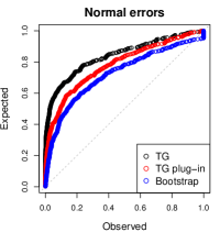
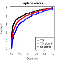
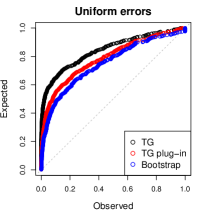
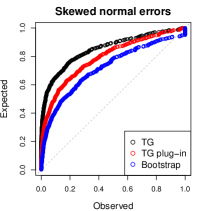
Step 2, p-values

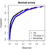
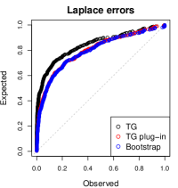
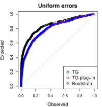
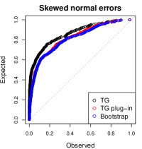
Step 3, p-values

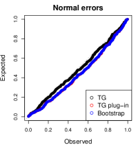
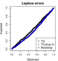
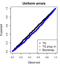
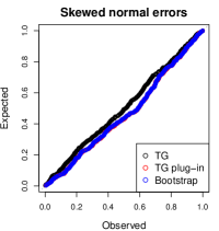
(a) P-values are shown, after each of 3 steps of LAR.

All steps, pivotal statistics

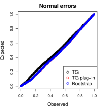
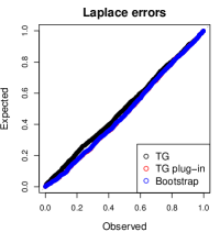
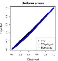
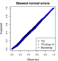
(b) Pivotal statistics are shown, aggregated over all 3 steps of LAR.

Figure 3: A simulation setup with $n=50$ and $d=10$, and a mean $\theta=X\beta_{0}$, where $\beta_{0}$ has 2 nonzero components.

Figure 3(b) inspects the TG statistic and plug-in and boostrap variants, when the pivot value $\mu$ is set to the true population value. That is, we set $\mu=v^{T}\theta$ in computing the statistics in (18), (19), and (20), in each data instance and each step of LAR. The figure collects the p-values across all 3 steps of LAR, for each of the 4 error distribution types. According to our theory, the distribution of the TG pivotal statistics here should be asymptotically uniform. This is clearly supported by the QQ plots. Interestingly, both plug-in and bootstrap pivotal statistics also appear uniform in the QQ plots, and yet, this is not a case handled by our asymptotic theory: recall, Theorem 11 fixes the pivot value $\mu$ to be 0 (as, otherwise, technical difficulties are encountered in its proof). This gives empirical evidence to the idea that a more refined analysis could extend Theorem 11 to the broader setting (of arbitrary pivot values) handled by Theorem 7. Moreover, it suggests that inverting the plug-in and bootstrap TG statistics should yield intervals with proper coverage, which is verified in the next subsection.

Lastly, we repeated all experiments in this subsection with the predictors $X\in\mathbb{R}^{50\times 10}$ generated in such a way to induce a (population) correlation of 0.5 between all pairs of predictor variables. The results are quite similar to those shown in Figure 3, and are hence deferred to Appendix A.12.

6.2 Confidence interval examples

We stay in same setting as the last subsection, so that $n=50$, $d=10$, and $\theta=X\beta_{0}$ for a coefficient vector $\beta_{0}$ with its first 2 components equal to $-4$ and $4$, and the rest equal to 0. We invert the TG, plug-in TG, and bootstrap TG statistics to obtain 90% confidence intervals at each LAR step. See Table 1 for a numerical summary. “Coverage” refers to the average fraction of intervals that contained their respective targets over the 500 repetitions, “power” is the average fraction of intervals that excluded zero, and “width” is the median interval width. These are all recorded in an unconditional sense, i.e., no screening of repetitions was performed based on the variables that were selected across the 3 steps of LAR (the conditional coverages however, were quite similar). From the table, we can see that all 3 methods lead to accurate coverage (around 90%) in all cases. We can further see that the intervals from the bootstrap TG statistic are shorter than those from the plug-in TG statistic in all cases, and considerably shorter than both the plug-in and original TG statistics in steps 2 and 3. The power from the bootstrap TG intervals is generally better than that from the plug-in TG intervals; also, it is on par with the power from the original TG statistic in step 1, but somewhat worse in step 2. Recall that the original TG statistic uses knowledge of the error variance ($\sigma^{2}=1$) but the bootstrap and plug-in variants do not.

N	TG
	Plug-in
	Boot
L	TG
	Plug-in
	Boot
U	TG
	Plug-in
	Boot
S	TG
	Plug-in
	Boot

Step 1
Coverage	Power	Width
0.914	0.508	5.622
0.928	0.378	7.561
0.932	0.528	5.477
0.904	0.568	5.193
0.944	0.410	7.271
0.944	0.566	5.429
0.912	0.538	5.153
0.928	0.396	7.284
0.924	0.540	5.453
0.892	0.540	5.346
0.940	0.402	7.210
0.936	0.520	5.477

Step 2
Coverage	Power	Width
0.890	0.520	10.309
0.914	0.404	15.774
0.916	0.424	7.856
0.926	0.536	11.153
0.930	0.440	14.859
0.944	0.454	7.892
0.902	0.504	12.347
0.910	0.390	17.497
0.910	0.422	7.808
0.878	0.504	10.876
0.896	0.380	15.687
0.912	0.394	8.060

Step 3
Coverage	Power	Width
0.910	0.114	25.155
0.918	0.100	34.642
0.930	0.090	9.141
0.912	0.118	26.393
0.904	0.120	36.206
0.924	0.108	9.273
0.894	0.128	26.451
0.886	0.126	39.299
0.892	0.118	8.913
0.906	0.116	26.592
0.910	0.106	38.965
0.918	0.102	9.057

Table 1: Summary statistics for 90% confidence intervals constructed in the problem setting of Figure 3. The 4 blocks of rows correspond to the 4 types of noise: normal, Laplace, uniform, and skew normal, respectively. The standard errors are about 0.01, 0.02, and 0.42 for the coverage, power, and width statistics, respectively.

It is a bit surprising that the bootstrap intervals can be shorter but still have worse power than the original TG intervals. This is easier to understand once the intervals are visualized, as done in Figure 4. The figure shows 100 sample intervals from the first LAR step, under normally distributed errors. Sample intervals from the other error models are shown in Appendix A.13. We see that the bootstrap TG intervals are indeed shorter, but compared to the original TG intervals, they are more symmetric around the target population values. The original TG intervals, being more asymmetric, are often shorter on the side (of the target value) facing 0, and this results in better power.

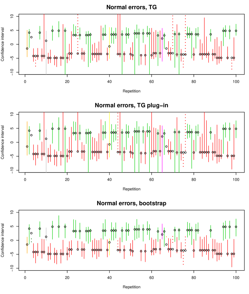
Figure 4: Confidence intervals from 100 draws of $Y$ from the same model as that in Figure 3. These intervals are constructed from the first step of LAR, under a uniform distribution for noise. The colors are simply a visual aid to mark the selection of different variables at step 1. The open circles denote the true population quantity to be covered (here, the coefficient from projecting $\theta$ onto the first selected variable). Intervals that do not contain their targets are drawn as dotted segments.

Again, we repeated the experiments here with the predictors $X\in\mathbb{R}^{50\times 10}$ generated to have pairwise correlation 0.5. Comparisons can be drawn between the results in a manner that roughly parallels the discussions following Table 1; however, on an absolute scale, all methods display a decrease in power across the board (as correlated predictors clearly make the problem more difficult). Details are provided in Appendix A.14.

6.3 Heteroskedastic errors

In the same setup as in Sections 6.1 and 6.2, with $n=50$, $d=10$, and the predictors $X$ and mean $\theta$ generated in the same manner, we consider a heteroskedastic model for $Y$ by drawing $\epsilon^{\prime}_{i}$, $i=1,\ldots,n$ i.i.d. from the given distribution—normal, Laplace, uniform, or skew normal—and then taking the errors to be $\epsilon_{i}=\sigma_{i}\epsilon_{i}^{\prime}$, $i=1,\ldots,n$, where $\sigma^{2}_{i}=10\|x_{i}\|_{2}^{2}$, $i=1,\ldots,n$ (and where $x_{i}\in\mathbb{R}^{d}$, $i=1,\ldots,n$ denote the rows of $X$.) The spread of error variances ended up being fairly substantial, from about 0.3 to 5.5. The original TG statistic was computed with $\sigma^{2}=\frac{1}{n}\sum_{i=1}^{n}\sigma_{i}^{2}$ as a surrogate for the common error variance; the plug-in and bootstrap variants were computed as usual. For brevity, we only plot the pivotal statistics, aggregated over 3 steps of LAR, in Figure 5. (This is analogous to what is shown in Figure 3(b) for the homoskedastic case. P-values at steps 1, 2, and 3, not shown, end up being similar to those in Figure 3(a), but the power from all methods is generally lower, due to the heteroskedastic errors.) As we can see, the pivotal statistics in the figure look very close to uniformly distributed, as desired. This is especially encouraging because the current problem setup lies outside of the scope of our asymptotic theory (which assumes a constant error variance), and it suggests that our theory could possibly be extended to accomodate errors with an (unknown) nonconstant variance structure.

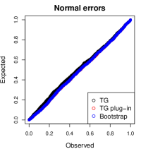
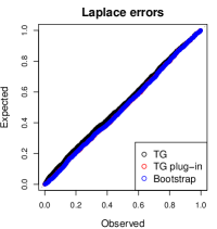
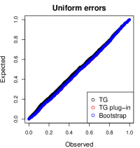
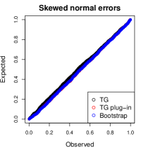
Figure 5: A simulation setup with $n=50$ and $d=10$, but with heteroskedastic errors. Shown are the pivotal statistics aggregated over 3 LAR steps.

6.4 High-dimensional examples

Finally, we consider a high-dimensional regime with $n=50$ and $d=1000$ predictors. The matrix $X\in\mathbb{R}^{50\times 1000}$ was generated according to the same recipe as before: each column, with equal probability, was assigned i.i.d. entries from $N(0,1)$, $\mathrm{Bern}(0.5)$, or $SN(0,1,5)$, and then scaled to have unit norm. The mean was defined as $\theta=X\beta_{0}$, where $\beta_{0}\in\mathbb{R}^{1000}$ has its first 2 components equal to -4 and 4, and the rest 0. Over 500 repetitions, a response $Y\in\mathbb{R}^{50}$ was generated by adding normal, Laplace, uniform, or skew normal noise to $\theta$, with an error variance of $\sigma^{2}=1$ (and every 10 repetitions, the predictor matrix $X$ was regenerated). Figure 6 plots the pivotal statistics aggregated over the first 3 steps of LAR. (This is as in Figure 3(b) for the low-dimensional case. P-values from the first 3 LAR steps are omitted for brevity, and are roughly similar to those in Figure 3(a), except that they display less power, due to the high-dimensionality.) The pivotal statistics here look quite close to uniform, as desired, and this is again encouraging, especially given that the current high-dimensional case lies outside of the scope of our theory (which assumes that $d$ is fixed). Further work on high-dimensional asymptotic theory should be pursued (see also Tian & Taylor (2017)), though, as we show in the next section, there is no hope for a uniform convergence result in high dimensions that holds as generally as the one we established in Theorem 7 for low dimensions.

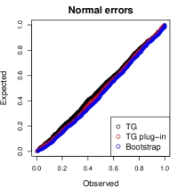
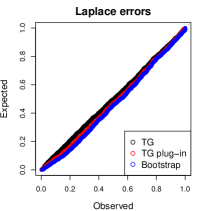
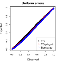
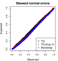
Figure 6: A simulation setup with $n=50$ and $d=1000$. Shown are the pivotal statistics over 3 LAR steps.

7 A negative result in high dimensions

We prove that the TG statistic fails to converge to a uniform distribution, under the null hypothesis, in a data model that has nonnormal errors and is high-dimensional, but otherwise represents a fairly standard setting: the “many means” setting. We write the observation model as

$$Y_{ij}=\mu_{j}+\epsilon_{ij},\;\;\;i=1,\ldots,m,\;j=1,\ldots,d,$$ (25)

where we interpret $i=1,\ldots,m$ as replications, and $j=1,\ldots,d$ as dimensions. In total there are hence $n=md$ observations. Denote

$$\overline{Y}_{j}=\frac{1}{m}\sum_{i=1}^{m}Y_{ij},\;\;\;j=1,\ldots,d.$$

We will analyze the TG statistic, when selection is performed based on the largest of $|\overline{Y}_{j}|$, $j=1,\ldots,d$, and inference is then performed on the corresponding mean parameter. A straightforward change of notation will translate the above into a regression problem, with an orthogonal design $X\in\mathbb{R}^{n\times d}$, but we stick with the many means formulation of the problem for simplicity.

We assume that the errors $\epsilon_{ij}$, $i=1,\ldots,m$, $j=1,\ldots,d$ in (25) are i.i.d. from the following mixture:

$$\pi\cdot N(-B,1)+(1-2\pi)\cdot N(0,1)+\pi\cdot N(B,1).$$ (26)

The mixing proportion $\pi$ and mean shift $B$ will both scale with $d$. Moreover, they will be chosen so that (for each $d$) the error variance is

$$\sigma^{2}=1+2\pi B^{2}=2.$$

As mentioned, we will consider model selection events of the form

$$\widehat{M}(Y)=(j,s)\iff s\overline{Y}_{j}\geq\max_{\ell\not=j}\;|\overline{Y}_{\ell}|.$$

We note that this is exactly the same selection event as that from the first step of FS, LAR, or lasso paths, when run on the regression version of this problem with orthogonal design $X$. It is not hard to check that the TG statistic for conditionally testing $\mu_{j}=0$, given that $\widehat{M}(Y)=(j,s)$, is

$$T(Y;j,s,0)=\frac{\displaystyle 1-\Phi\Bigg{(}\frac{\sqrt{m}s\overline{Y}_{j}}{\sqrt{2}}\Bigg{)}}{\displaystyle 1-\Phi\Bigg{(}\frac{\max_{\ell\not=j}\;\sqrt{m}|\overline{Y}_{\ell}|}{\sqrt{2}}\Bigg{)}}.$$ (27)

As per the spirit of our paper, we can also view this statistic unconditionally; for this it is helpful to define $W_{1}=|\overline{Y}_{1}|,\ldots,W_{d}=|\overline{Y}_{d}|$, and denote by $W_{(1)}\geq\ldots\geq W_{(d)}$ the order statistics. Then from (27), we can see that the unconditional TG statistic for testing the selected mean being 0 is

$$\pazocal{T}(Y;0)=\frac{\displaystyle 1-\Phi\Bigg{(}\frac{\sqrt{m}W_{(1)}}{\sqrt{2}}\Bigg{)}}{\displaystyle 1-\Phi\Bigg{(}\frac{\sqrt{m}W_{(2)}}{\sqrt{2}}\Bigg{)}}.$$ (28)

The framework underlying the TG statistic tells us that if the errors in (25) are i.i.d. $N(0,2)$, then for any fixed model $(j,s)$, the pivot $T(Y;j,s,0)$ is uniformly distributed conditional on $\widehat{M}(Y)=(j,s)$. Further, if $W_{(1)}$ and $W_{(2)}$ are the largest and second largest absolute values of centered normal random variables (each with variance $2/m$), then the unconditional pivot $\pazocal{T}(Y;0)$ is again uniform. But when $W_{(1)},W_{(2)}$ are large, and are defined by the order statistics of nonnormal random variates, the statistic $\pazocal{T}(Y;0)$—which in this case is defined by the extreme tail behavior of the normal distribution—could be nonuniform. The next theorem asserts that such nonuniformity does indeed happen asymptotically if we choose the mixture distribution in (26) appropriately.

Theorem 12.

Assume the observation model (25), where the errors are all drawn i.i.d. from (26). Let $d$ and $m$ scale in such a manner that $(\log{d})/m\to\infty$. Further, let

$$\pi=\Bigg{(}\frac{1}{d}\Bigg{)}^{1/m},\;\;\;B=\sqrt{\frac{d^{1/m}}{2}},$$

so that the error variance is fixed at $\sigma^{2}=2$. Then under the global null hypothesis, $\mu=0$, the unconditional TG statistic $\pazocal{T}(Y;0)$ in (28) does not converge in distribution to $U(0,1)$. In particular, on an event whose limiting probability is at least $1/e$, the statistic $\pazocal{T}(Y;0)$ converges to 0.

Further, the same results hold conditionally on any selected model. That is, for any fixed $(j,s)$, the conditional TG statistic $T(Y;j,s,0)\,|\,\widehat{M}(Y)=(j,s)$ does not converge in distribution to $U(0,1)$, and on an event with limiting probability (conditional on $\widehat{M}(Y)=(j,s)$) at least $1/e$, it converges to 0.

Remark 4.

The assumed condition $(\log d)/m\to\infty$ requires the dimension $d$ to diverge to $\infty$, but not necessarily the number of replications $m$, though it clearly allows $m$ to diverge at a sufficiently slow rate. On the other hand, if $d$ were fixed and $m$ diverged to $\infty$, then the result of the theorem would no longer be true, and the limiting distribution of the TG p-value would revert to $U(0,1)$. (To be careful, here we would have cap the mixing probability $\pi$ at $1/2$ in order for the mixture to make sense, since the current definition of $\pi$ diverges with $d$ fixed and $m$ tending to $\infty$.) In fact, this is ensured by our low-dimensional result in Theorem 7: after reformulating the many means problem in appropriate regression notation, all of the conditions of Theorem 7 are met by our current setup when $d$ is fixed. This is supported by the simulation in Figure 7.

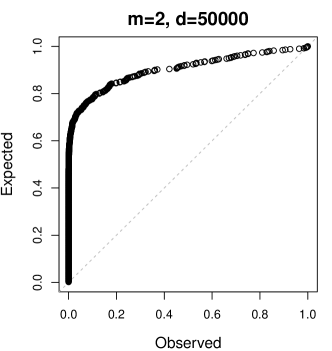
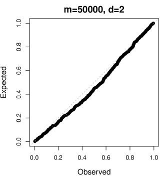
Figure 7: The left plot shows a QQ plot of TG p-values, computed over 500 repetitions from the many means setup exactly as described in Theorem 12, with $d=50,000$ and $m=2$. We can see that the p-values are clearly nonuniform, and $34\%$ of the p-values are 0 (up to computer precision), close to the theoretically predicted proportion of $1/e$. The right plot shows p-values from the same model, but having reversed the roles of $d$ and $m$ (we also had to cap $\pi$ at 1/2); we can see that the p-values are essentially uniform.

Remark 5.

The precise scaling $(\log d)/m\to\infty$ is chosen since this implies $\pi=(1/d)^{1/m}\to 0$, i.e., the extreme mixture components $N(-B,1)$ and $N(B,1)$ each have probability tending to 0, an intuitively reasonable property for the error distribution. But we note that this scaling is not important for any other reason, and the proof would still remain correct if $d/m\to\infty$.

Remark 6.

In Theorem 3 of Tian & Taylor (2017), the authors show that the TG statistic converges in distribution to a standard uniform random variable, in a high-dimensional problem setting, with some restrictions on the sequences of selection events that are allowed. One might ask what part of our high-dimensional setup here violates their conditions, because both results obviously cannot be true simultaneously. As far as we can tell, the issue lies in the role of $\delta_{n}$ in Assumption 1 of Tian & Taylor (2017). Namely, as we have defined the error distribution in (26), the value of $\delta_{n}$ needed to certify the third condition Assumption 1 of their work is too small for the main assumption in their Theorem 3 to hold. Hence Theorem 3 of Tian & Taylor (2017) does not apply to our current setup.

8 Discussion

We have studied the selective pivotal inference framework, with a focus on forward stepwise regression (FS), least angle regression (LAR), and the lasso, in regression problems with nonnormal errors. We have shown that the truncated Gaussian (TG) pivot is asymptotically robust in low-dimensional settings to departures from normality, in that it converges to a $U(0,1)$ distribution (its pivotal distribution under normality), and does so uniformly over a broad class of nonnormal error distributions. When the error variance $\sigma^{2}$ is unknown, we have proposed plug-in and bootstrap versions of the TG statistic, both of which yield provably conservative asymptotic p-values.

Our numerical experiments revealed that the statistics under theoretical investigation generally display excellent finite-sample performance, for highly nonnormal error distributions. These experiments also revealed findings not predicted by our theory: (i) the bootstrap TG statistic often produces shorter confidence intervals than those based on the plug-in TG statistic, and even the TG statistic that relies on the error variance $\sigma^{2}$; and (ii) all three TG statistics show strong empirical properties well-outside of the classic homoskedastic, fixed $d$ regression setting that we presumed theoretically.

However, as we have clearly demonstrated, one should not hope for a convergence result in high dimensions that is as general as the result obtained in low dimensions. In a relatively simple many means problem, we showed the nonconvergence of the TG statistic to $U(0,1)$ as $d\to\infty$, whereas in the same problem but with $d$ fixed, the TG statistic converges to its usual $U(0,1)$ limit.

There is still much left to do in terms of understanding the behavior of selective pivotal inference tools that are constructed to have exact finite-sample guarantees under normality, like the TG statistic of Tibshirani et al. (2016), when applied in high-dimensional regression settings with nonnormal data. When the pivot, the central cog of this framework, is constructed under the assumption of normality, this creates robustness issues that are especially worrisome in high dimensions. Appendix A.16 provides a high-level discussion of some of these issues; a more detailed study will be the subject of future research.

Acknolwedgements

We thank Jelena Markovic and Jonathan Taylor for many helpful discussions, and for their overall generosity. An initial version of our work contained only unconditional (i.e., marginal) results in the main theorems (Theorems 7, 11, and 12); Jelena Markovic pointed out that Theorem 7 should also hold conditionally, and the current version of this work has been revised accordingly.

Appendix A Appendix

A.1 Convex cones for FS, LAR, lasso

We describe a modification of the conic conditioning set in Tibshirani et al. (2016) for FS. Our version is different in that we additionally condition on the sign of every active coefficient at every step, rather than just the coefficient of the variable to enter the model at each step. The modifications needed for the LAR and lasso conditioning sets, made on top of the sets for LAR and lasso given in Tibshirani et al. (2016), will follow similarly to that described for FS, and hence we omit the details.

After $k$ FS steps, we can always represent a sequence of active sets $\widehat{A}_{\ell}(y)$, $\ell=1,\ldots,k$ by a sorted list of variables $[\widehat{j}_{1}(y),\ldots,\widehat{j}_{k}(y)]$ that were chosen to enter the model at each step. Unfortunately, the same cannot be done for a sequence of active signs $\widehat{s}_{\ell}(y)$, $\ell=1,\ldots,k$, because these do not obey such a nested structure. We will write $\widehat{s}_{\ell}(y)=[\widehat{s}_{\ell,1}(y),\ldots\widehat{s}_{\ell,\ell}(y)]$ for the signs of coefficients corresponding to the variables $[\widehat{j}_{1}(y),\ldots,\widehat{j}_{\ell}(y)]$, at the $\ell$th step.

Now we characterize the event that $\widehat{A}_{\ell}(y)=A_{\ell}$, $\widehat{s}_{\ell}(y)=s_{\ell}$, for $\ell=1,\ldots,k$, using induction. At step $\ell=1$, we have that $\widehat{j}_{1}(y)=j_{1}$ and $\widehat{s}_{1}(y)=s_{1}$ if and only if

$$s_{1}X_{j_{1}}^{T}y/\|X_{j_{1}}\|_{2}^{2}\geq\pm X_{j}^{T}y/\|X_{j}\|_{2}^{2}\;\;\;\text{for all $j\not=j_{1}$},$$

or, rearranged,

$$\big{(}s_{1}X_{j_{1}}/\|X_{j_{1}}\|_{2}^{2}\pm X_{j}/\|X_{j}\|_{2}^{2}\big{)}^{T}y\geq 0\;\;\;\text{for all $j\not=j_{1}$},$$

a set of $2(d-1)$ linear inequalities in $y$. Assume that we have represented the event that $\widehat{A}_{\ell}(y)=A_{\ell}$ and $\widehat{s}_{\ell}(y)=s_{\ell}$, for $\ell=1,\ldots,k-1$, by a collection of linear inequalities in $y$. Then to represent $\widehat{j}_{k}(y)=j_{k}$ and $\widehat{s}_{k}(y)=[s_{k,1},\ldots,s_{k,k}]$, we must only append to this collection of inequalities. The former subevent $\widehat{j}_{k}(y)=j_{k}$ is characterized by

$$\big{(}s_{k,k}\widetilde{X}_{j_{k}}/\|\widetilde{X}_{j_{k}}\|_{2}^{2}\pm\widetilde{X}_{j}/\|\widetilde{X}_{j}\|_{2}^{2}\big{)}^{T}r\geq 0\;\;\;\text{for all $j\not=j_{1},\ldots,j_{k}$},$$

where $\widetilde{X}_{j}$ is the residual from regressing $X_{j}$ onto $X_{A_{k-1}}$, and $r$ is the residual from regression $y$ onto $X_{A_{k-1}}$. By expressing $\widetilde{X}_{j}=P_{A_{k-1}}^{\perp}X_{j}$ and $r=P_{A_{k-1}}^{\perp}X_{j}$, where $P_{A_{k-1}}^{\perp}$ projects onto the orthocomplement of the column space of $X_{A_{k-1}}$, we can rewrite the above constraints as

$$\big{(}s_{k,k}P_{A_{k-1}}^{\perp}X_{j_{k}}/\|P_{A_{k-1}}^{\perp}X_{j_{k}}\|_{2}^{2}\pm P_{A_{k-1}}^{\perp}X_{j}/\|P_{A_{k-1}}^{\perp}X_{j}\|_{2}^{2}\big{)}^{T}y\geq 0\;\;\;\text{for all $j\not=j_{1},\ldots,j_{k}$},$$

a set of $2(d-k)$ linear inequalities in $y$. Meanwhile, the subevent $\widehat{s}_{k}(y)=[s_{k,1},\ldots,s_{k,k}]$ can be characterized by $k$ inequalities expressed in block form,

$$\mathrm{diag}(s_{1,1},\ldots,s_{k,k})\,(X_{A_{k}}^{T}X_{A_{k}})^{-1}X_{A_{k}}^{T}y\geq 0.$$

This completes the proof.

A.2 Proof of Lemma 3

We prove the result for FS; the results for the LAR and lasso paths follows similarly, by inpsecting the form of the linear inequalities that determine their selection events.

Consider the first FS step as described in Appendix A.1. Multiplying through by $\sqrt{n}$, we see that an equivalent set of inequalities that characterize the selection event $\widehat{j}_{1}(y)=j_{1}$, $\widehat{s}_{1}(y)=s_{1}$ is

$$s_{1}\frac{n}{X_{j_{1}}^{T}X_{j_{1}}}\frac{X_{j_{1}}^{T}y}{\sqrt{n}}\pm\frac{n}{X_{j}^{T}X_{j}}\frac{X_{j}^{T}y}{\sqrt{n}}\geq 0\;\;\;\text{for all $j\not=j_{1}$}.$$

This is clearly of the desired form $P_{1}(\frac{1}{n}X^{T}X)\,\frac{1}{\sqrt{n}}X^{T}y\geq 0$, for a matrix $P_{1}(\frac{1}{n}X^{T}X)$ dependent only on $\frac{1}{n}X^{T}X$. At the $k$th step of FS, there are two sets of inequalities to be examined: one that describes the variable to enter $\widehat{j}_{k}(y)=j_{k}$, and the second that describes the active signs $\widehat{s}_{k}(y)=[s_{k,1},\ldots,s_{k,k}]$. The first set, multiplying through by $\sqrt{n}$, is

$$s_{k,k}\frac{nX_{j_{k}}^{T}X_{A_{k-1}}(X_{A_{k-1}^{T}}X_{A_{k-1}})^{-1}}{X_{j_{k}}^{T}X_{A_{k-1}}(X_{A_{k-1}^{T}}X_{A_{k-1}})^{-1}X_{A_{k-1}}^{T}X_{j_{k}}}\frac{X_{A}^{T}y}{\sqrt{n}}\pm\frac{nX_{j}^{T}X_{A_{k-1}}(X_{A_{k-1}^{T}}X_{A_{k-1}})^{-1}}{X_{j}^{T}X_{A_{k-1}}(X_{A_{k-1}^{T}}X_{A_{k-1}})^{-1}X_{A_{k-1}}^{T}X_{j}}\frac{X_{A}^{T}y}{\sqrt{n}}\geq 0\\ \text{for all $j\not=j_{1},\ldots,j_{k}$},$$

while the second set, again multiplying through by $\sqrt{n}$, is

$$\mathrm{diag}(s_{1,1},\ldots,s_{k,k})\,n(X_{A_{k}}^{T}X_{A_{k}})^{-1}\frac{X_{A_{k}}^{T}y}{\sqrt{n}}\geq 0.$$

These inequalities are clearly all summarized by $P_{k}(\frac{1}{n}X^{T}X)\,\frac{1}{\sqrt{n}}X^{T}y\geq 0$, where $P_{k}(\frac{1}{n}X^{T}X)$ is a matrix that depends only on $\frac{1}{n}X^{T}X$. This completes the proof.

A.3 Proof of Lemma 4

Under the conditions of the lemma, the TG pivot for fixed $M$ in (8) depends only on $X,y$ through the master statistic, because, as explained above the lemma, the only dependence in the pivot on $X,y$ is through the quantities $v^{T}y/\|v\|_{2}$, $(Q_{M}(X)\,v)/\|v\|_{2}$, $Q_{M}(X)\,y$, and each of these is in turn a function of the master statistic $\Omega_{n}$. Moreover, we may reexpress the TG statistic in (10) as

$$T(X,y;M,v,\mu)=\frac{\Phi\big{(}f_{1}(\frac{1}{n}X^{T}X,\frac{1}{\sqrt{n}}X^{T}y)\big{)}-\Phi\big{(}f_{2}(\frac{1}{n}X^{T}X,\frac{1}{\sqrt{n}}X^{T}y)\big{)}}{\Phi\big{(}f_{1}(\frac{1}{n}X^{T}X,\frac{1}{\sqrt{n}}X^{T}y)\big{)}-\Phi\big{(}f_{3}(\frac{1}{n}X^{T}X,\frac{1}{\sqrt{n}}X^{T}y)\big{)}},$$

for some functions $f_{1},f_{2},f_{3}$, or more succinctly, as $T(X,y;M,v,\mu)=\psi_{M}(\frac{1}{n}X^{T}X,\frac{1}{\sqrt{n}}X^{T}y)$, where

$$\psi_{M}(S,z)=\frac{\Phi\big{(}f_{1}(S,z)\big{)}-\Phi\big{(}f_{2}(S,z)\big{)}}{\Phi\big{(}f_{1}(S,z)\big{)}-\Phi\big{(}f_{3}(S,z)\big{)}}.$$

Note that the quantities $v^{T}y/\|v\|_{2}$, $(Q_{M}(X)\,v)/\|v\|_{2}$, $Q_{M}(X)\,y$ depend smoothly on the master statistic $\Omega_{n}=(\frac{1}{n}X^{T}X,\frac{1}{\sqrt{n}}X^{T}y)$ at any point such that $\frac{1}{n}X^{T}X$ is nonsingular. This implies $f_{1},f_{2},f_{3}$ are smooth functions of $(S,z)$ at any point such that $S$ is nonsingular. Lastly, for all $S,z$ such that $P_{M}(S)\,z>0$, we have $f_{1}(S,z)>f_{3}(S,z)$, and thus the denominator of $\phi_{M}(S,z)$ is positive. This proves the desired continuity result on $\psi_{M}$.

A.4 Proof of Lemma 5

For the master statistic $\Omega_{n}=(\frac{1}{n}X^{T}X,\frac{1}{\sqrt{n}}X^{T}Y)$, note that $\mathbb{E}(\Omega_{n})=(\frac{1}{n}X^{T}X,\frac{1}{\sqrt{n}}X^{T}\theta)$. As $v$ is assumed to be chosen such that $v^{T}\theta$ is a normalized regression coefficient from the projection of $\theta$ onto some subset of the columns in $X$, we may assume without a loss of generality that $v^{T}\theta$ is as in (7) for some $A,j$. Then, we see that we must only define

$$g(S,z)=\frac{e_{j}^{T}(S_{A,A})^{-1}z_{A}}{\sqrt{e_{j}^{T}(S_{A,A})^{-1}e_{j}}},$$

where we use $S_{A,A}$ to denote the submatrix of $S$ with rows in $A$ and columns in $A$, and $z_{A}$ to denote the subvector of $z$ with entries in $A$.

A.5 Proof of Lemma 6

Define $Z_{0,n}=\sum_{i=1}^{n}\xi_{i}$, where $\xi_{i}=\frac{1}{\sqrt{n}}x_{i}\epsilon_{i}$, $x_{i}$ is the $i$th row of $X$, and $\epsilon_{i}=Y_{i}-\theta_{i}$, for $i=1,\ldots,n$. Note that $(\xi_{1},\ldots,\xi_{n})\sim F_{n}(0)$, with independent, mean zero components. We compute

$$\sum_{i=1}^{n}\mathrm{Cov}(\xi_{i})=\frac{\sigma^{2}}{n}\sum_{i=1}^{n}x_{i}x_{i}^{T}=\frac{\sigma^{2}}{n}X^{T}X,$$

which converges to $\sigma^{2}\Sigma$ as $n\to\infty$, by assumption. Further, for any $\delta>0$, consider

$$\sum_{i=1}^{n}\mathbb{E}\Big{(}\|\xi_{i}\|_{2}^{2}\cdot 1\{\|\xi_{i}\|_{2}\geq\delta\}\Big{)}=\frac{1}{n}\sum_{i=1}^{n}\|x_{i}\|_{2}^{2}\;\mathbb{E}\Bigg{(}\epsilon_{i}^{2}\cdot 1\Bigg{\{}\frac{\|x_{i}\|_{2}}{\sqrt{n}}|\epsilon_{i}|\geq\delta\Bigg{\}}\Bigg{)}.$$

We seek to show that this converges to 0 as $n\to\infty$. As $\frac{1}{n}\sum_{i=1}^{n}\|x_{i}\|_{2}^{2}\to\mathrm{tr}(\Sigma)$, it suffices to show that the maximum of the above expectations (in the summands) converges to 0, which is implied by the assumption that $\max_{i=1,\ldots,n}\|x_{i}\|_{2}/\sqrt{n}\to 0$. As the above arguments did not depend on the sequence $F_{n}(0)$, $n=1,2,3,\ldots$, we have verified the Lindeberg-Feller conditions uniformly, and hence the uniform Lindeberg-Feller central limit theorem, Lemma 2, implies that $Z_{0,n}$ converges in distribution to $Z_{0}\sim N(0,\sigma^{2}\Sigma)$, uniformly over $\pazocal{P}_{n}(0)$.

Now consider $Z_{n}=\frac{1}{\sqrt{n}}X^{T}Y=Z_{0,n}+\frac{1}{\sqrt{n}}X^{T}\theta$. Writing $\Phi$ and $\phi$ for the standard normal CDF and density,

$$\sup_{\theta\in\Theta}\;\sup_{F_{n}(\theta)\in\pazocal{P}_{n}(\theta)}\;\sup_{x\in\mathbb{R}^{d}}\; \big{|}\mathbb{P}(Z_{n}\leq x)-\mathbb{P}(Z\leq x)\big{|}$$

$$=\sup_{\theta\in\Theta}\;\sup_{F_{n}(\theta)\in\pazocal{P}_{n}(\theta)}\;\sup_{x\in\mathbb{R}^{d}}\;\Bigg{|}\mathbb{P}\Bigg{(}Z_{0,n}\leq x-\frac{1}{\sqrt{n}}X^{T}\theta\Bigg{)}-\mathbb{P}(Z\leq x)\Bigg{|}$$

$$\leq\sup_{\theta\in\Theta}\;\sup_{F_{n}(\theta)\in\pazocal{P}_{n}(\theta)}\;\sup_{x\in\mathbb{R}^{d}}\;\big{|}\mathbb{P}(Z_{0,n}\leq x)-\mathbb{P}(Z_{0}\leq x)\big{|}\;+\;\sup_{x\in\mathbb{R}^{d}}\;\Bigg{|}\Phi(x-\eta)-\Phi\Bigg{(}x-\frac{1}{\sqrt{n}}X^{T}\theta\Bigg{)}\Bigg{|}$$

$$\leq\underbrace{\sup_{\theta\in\Theta}\;\sup_{F_{n}(\theta)\in\pazocal{P}_{n}(\theta)}\;\sup_{x\in\mathbb{R}^{d}}\;\big{|}\mathbb{P}(Z_{0,n}\leq x)-\mathbb{P}(Z_{0}\leq x)\big{|}}_{a}\;+\;\underbrace{\vphantom{\sup_{x\in\mathbb{R}^{d}}}\Bigg{|}\frac{1}{\sqrt{n}}X^{T}\theta-\eta\Bigg{|}\phi(0)}_{b},$$

where the second line is due to the triangle inequality, and the third line is due to the simple bound $|\Phi(x-t)-\Phi(x-s)|=|\int_{x-s}^{x-t}\phi(u)\,du|\leq|t-s|\phi(0)$, for any $x,s,t$. Note that $a\to 0$ by the argument at the start of this proof, and $b\to 0$ by assumption in (17). This shows that $Z_{n}$ converges in distribution to $Z\sim N(\eta,\sigma^{2}\Sigma)$, uniformly over $\pazocal{P}_{n}(\theta)$, and over $\theta\in\Theta$.

Lastly, we establish the conditional result. By repeating the same arguments as above, the uniform Lindeberg-Feller central limit theorem and condition (17) imply that $(Z_{n},A_{n}Z_{n})$ converges to $(Z,AZ)$, uniformly over $\pazocal{P}_{n}(\theta)$, and over $\theta\in\Theta$. Thus, along sequence $F_{n}(\theta)\in\pazocal{P}_{n}(\theta)$, $n=1,2,3,\ldots$ with $\theta\in\Theta$, observe

$$\mathbb{P}(Z_{n}\leq x\,|\,A_{n}Z_{n}\geq 0)=\frac{\mathbb{P}(Z_{n}\leq x,\,A_{n}Z_{n}\geq 0)}{\mathbb{P}(A_{n}Z_{n}\geq 0)}\to\frac{\mathbb{P}(Z\leq x,\,AZ\geq 0)}{\mathbb{P}(AZ\geq 0)},$$

at a rate that does not depend on the sequence in question. This is true because the numerator and denominator each converge to their normal probability counterparts, and the denominator remains bounded away from zero since $\{z:Az\geq 0\}$ has nonempty interior, and the set of limits of $\frac{1}{\sqrt{n}}X^{T}\theta$ was assumed compact, in (17). Since $x$ was arbitrary, and the distribution of $Z\,|\,AZ\geq 0$ is continuous, we have (e.g., Lemma 2.11 in van der Vaart (1998))

$$\sup_{x\in\mathbb{R}^{d}}\;\Big{|}\mathbb{P}(Z_{n}\leq x\,|\,A_{n}Z_{n}\geq 0)-\mathbb{P}(Z\leq x\,|\,AZ\geq 0)\Big{|}\to 0.$$

And as the sequence $F_{n}(\theta)\in\pazocal{P}_{n}(\theta)$, $n=1,2,3,\ldots$ with $\theta\in\Theta$ was arbitrary, we have shown the desired uniform convergence.

A.6 Proof of Theorem 7

We begin with the proof of part (a). Let $Z_{n}=\frac{1}{\sqrt{n}}X^{T}Y$ and $Z\sim N(\eta,\sigma^{2}\Sigma)$. Also, let $A_{n}=P_{M}(\frac{1}{n}X^{T}X)$ and $A=P_{M}(\Sigma)$. Recall that $A_{n}Z_{n}\geq 0\iff\widehat{M}(X,Y)=M$, by Lemma 3. Also, $Z_{n}\,|\,A_{n}Z_{n}\geq 0$ converges weakly to $Z\,|\,AZ\geq 0$, uniformly over $\pazocal{P}_{n}(\theta)$ and over $\theta\in\Theta$, by Lemma 6. As $\frac{1}{n}X^{T}X\to\Sigma$ deterministically, we also have that $\Omega_{n}=(\frac{1}{n}X^{T}X,Z_{n})$ converges uniformly in distribution to $\Omega=(\Sigma,Z)$.

The choice of $v$ as specified in the theorem is now important for two reasons. First, by Lemma 4, we can express

$$T(X,Y;M,v,\mu)=\psi_{M}(\Omega_{n}),$$

for a function $\psi_{M}$. Second, by Lemma 5, we can express $v^{T}\theta=g(\mathbb{E}(\Omega_{n}))$ for a function $g$. Neither $\psi_{M}$ nor $g$ depend on $n$, and the distribution in question is that of $\psi_{M}(\Omega_{n})\,|\,A_{n}Z_{n}\geq 0$ under $g(\mathbb{E}(\Omega_{n}))=\mu$. The function $\psi_{M}$ is continuous at any point $(S,z)$ such that $S$ is nonsingular and $Az>0$; recalling the assumed nonsingularity of $\Sigma$, it is therefore continuous on a set of full probability under the limiting distribution $\pazocal{L}(\Omega\,|\,AZ\geq 0)$. By the uniform continuous mapping theorem, Lemma 1, $\psi_{M}(\Omega_{n})\,|\,A_{n}Z_{n}\geq 0$ converges uniformly to $\psi(\Omega)\,|\,AZ\geq 0$, which is distributed as $U(0,1)$ when $g(\mathbb{E}(\Omega))=\mu$ by the pivotal property of the TG statistic under normality, as in (8). The proof of uniform validity of TG confidence intervals is just a rearrangement of the uniform asymptotic pivotal statement.

The proof of part (b) follows from the expansion

$$\pazocal{T}(X,Y;V,U)=\sum_{M\in\pazocal{M}}T(X,Y;M,v_{M},\mu_{M})\,1\{\widehat{M}(X,Y)=M\}.$$

As the number possible models $|\pazocal{M}|$ is finite, we can simply apply the asymptotic pivotal result from part (a) to each $M\in\pazocal{M}$ to establish the asymptotic pivotal property of $\pazocal{T}(X,Y;V,U)$. The confidence interval result is again just a rearrangement of this pivotal property.

A.7 Proof of Lemma 8

By assumption, the vector $v$ can be written as

$$v=\frac{X_{A}(X_{A}^{T}X_{A})^{-1}e_{j}}{\sqrt{e_{j}^{T}(X_{A}^{T}X_{A})^{-1}e_{j}}},$$

for some $A,j$. We compute

$$\|v\|_{3}^{3} =\frac{\sum_{i=1}^{n}|X_{i,A}(X_{A}^{T}X_{A})^{-1}e_{j}|^{3}}{|e_{j}^{T}(X_{A}^{T}X_{A})^{-1}e_{j}|^{3/2}}$$

$$=\frac{\frac{1}{n^{3/2}}\sum_{i=1}^{n}|X_{i,A}n(X_{A}^{T}X_{A})^{-1}e_{j}|^{3}}{|e_{j}^{T}n(X_{A}^{T}X_{A})^{-1}e_{j}|^{3/2}}.$$

The denominator converges to $|e_{j}^{T}(\Sigma_{A,A})^{-1}e_{j}|^{3/2}$ by (14). The numerator satisfies

$$\frac{1}{n^{3/2}}\sum_{i=1}^{n}|X_{i,A}n(X_{A}^{T}X_{A})^{-1}e_{j}|^{3}\leq\frac{1}{\sqrt{n}}\;\cdot\;\underbrace{\frac{1}{n}\sum_{i=1}^{n}\|x_{i}\|_{2}^{3}}_{a}\;\cdot\;\underbrace{\vphantom{\frac{1}{n}\sum_{i=1}^{n}}\|n(X_{A}^{T}X_{A})^{-1}e_{j}\|_{2}^{3}}_{b},$$

where $a$ is bounded by (21) and $b$ converges to $\|(\Sigma_{A,A})^{-1}e_{j}\|_{2}^{3}$ by (14). This completes the proof.

A.8 Proof of Lemma 9

We start by proving the result about the event $\{cs_{Y}\geq\sigma\}$. First let us study its asymptotic probability marginally. Consider

$$\mathbb{E}(s_{Y}^{2}) =\frac{1}{n}\sum_{i=1}^{n}\mathbb{E}|\epsilon_{i}+\theta_{i}-\overline{\epsilon}-\overline{\theta}|^{2}$$

$$=\frac{1}{n}\sum_{i=1}^{n}\mathbb{E}|\epsilon_{i}-\overline{\epsilon}|^{2}+\frac{1}{n}\sum_{i=1}^{n}|\theta_{i}-\overline{\theta}|^{2}+\frac{2}{n}\sum_{i=1}^{n}\mathbb{E}(\epsilon_{i}-\overline{\epsilon})(\theta_{i}-\overline{\theta})$$

$$=\frac{n-1}{n}\sigma^{2}+s_{\theta}^{2},$$

where $\overline{\epsilon}=\sum_{i=1}^{n}\epsilon_{i}/n$. Hence

$$\mathbb{P}\big{(}cs_{Y}\leq\sigma\big{)} =\mathbb{P}\big{(}c^{2}s_{Y}^{2}-c^{2}\mathbb{E}(s_{Y}^{2})\leq\sigma^{2}-c^{2}\mathbb{E}(s_{Y}^{2})\big{)}$$

$$\leq\frac{c^{4}\mathrm{Var}(s_{Y}^{2})}{(c^{2}\mathbb{E}(s_{Y}^{2})-\sigma^{2})^{2}},$$

where in the last line we used Chebyshev’s inequality. Recalling that $c^{2}>1$, we have the lower bound $(c^{2}\mathbb{E}(s_{Y}^{2})-\sigma^{2})^{2}\geq 0.999(c^{2}-1)^{2}\sigma^{4}$, for $n$ large enough. Therefore, to show $\mathbb{P}(cs_{Y}\geq\sigma)\to 1$, it is enough to show that $\mathrm{Var}(s_{Y}^{2})\to 0$ as $n\to\infty$, uniformly. For this, we will use the simple inequality

$$\mathrm{Var}(W_{1}+\ldots+W_{m})\leq m\sum_{i=1}^{m}\mathrm{Var}(W_{i}),$$ (29)

which follows from the fact that $2\mathrm{Cov}(W_{i},W_{j})\leq\mathrm{Var}(W_{i})+\mathrm{Var}(W_{j})$. We will also invoke Rosenthal’s inequality (Rosenthal, 1970), which for independent $W_{1},\ldots,W_{m}$, having mean zero and $\mathbb{E}|W_{i}|^{t}<\infty$ for $i=1,\ldots,m$, states that

$$\mathbb{E}\Bigg{|}\sum_{i=1}^{m}W_{i}\Bigg{|}^{t}\leq C_{t}\max\Bigg{\{}\sum_{i=1}^{m}\mathbb{E}|W_{i}|^{t},\;\Bigg{(}\sum_{i=1}^{m}\mathbb{E}W_{i}^{2}\Bigg{)}^{t/2}\Bigg{\}},$$ (30)

for a constant $C_{t}>0$ only depending on $t$. Hence, observe that

$$\mathrm{Var}(s_{Y}^{2}) =\mathrm{Var}\Bigg{(}\frac{1}{n}\sum_{i=1}^{n}|\epsilon_{i}+\theta_{i}-\overline{\epsilon}-\overline{\theta}|^{2}\Bigg{)}$$

$$=\mathrm{Var}\Bigg{(}\frac{1}{n}\sum_{i=1}^{n}|\epsilon_{i}+\theta_{i}-\overline{\theta}|^{2}+\overline{\epsilon}^{2}-\frac{2}{n}\sum_{i=1}^{n}(\epsilon_{i}+\theta_{i}-\overline{\theta})\overline{\epsilon}\Bigg{)}$$

$$=\mathrm{Var}\Bigg{(}\frac{1}{n}\sum_{i=1}^{n}|\epsilon_{i}+\theta_{i}-\overline{\theta}|^{2}-\overline{\epsilon}^{2}\Bigg{)}$$

$$\leq\underbrace{2\mathrm{Var}\Bigg{(}\frac{1}{n}\sum_{i=1}^{n}|\epsilon_{i}+\theta_{i}-\overline{\theta}|^{2}\Bigg{)}}_{a}+\underbrace{\vphantom{\Bigg{(}\frac{1}{n}\sum_{i=1}^{n}\Bigg{|}}2\mathrm{Var}(\overline{\epsilon}^{2})}_{b},$$

where in the last line we used (29). We consider $a,b$ individually. We have

$$a =\frac{2}{n^{2}}\mathrm{Var}\Bigg{(}\sum_{i=1}^{n}\epsilon_{i}^{2}+\sum_{i=1}^{n}|\theta_{i}-\overline{\theta}|^{2}+2\sum_{i=1}^{n}\epsilon_{i}(\theta_{i}-\overline{\theta})\Bigg{)}$$

$$\leq\frac{6}{n^{2}}\mathrm{Var}\Bigg{(}\sum_{i=1}^{n}\epsilon_{i}^{2}\Bigg{)}+\frac{12}{n^{2}}\mathrm{Var}\Bigg{(}\sum_{i=1}^{n}\epsilon_{i}(\theta_{i}-\overline{\theta})\Bigg{)}$$

$$\leq\frac{6}{n}\kappa+\frac{12}{n}\sigma^{2}s_{\theta}^{2}\to 0,$$

where the second line again used (29), and the third used our assumptions on the error distribution in (22), and on $\theta$ in (24). We also have

$$b =\frac{2}{n^{4}}\mathbb{E}\Bigg{|}\sum_{i=1}^{n}\epsilon_{i}\Bigg{|}^{4}$$

$$\leq\frac{2}{n^{4}}C_{4}\max\{n\kappa,n^{2}\sigma^{4}\}\to 0,$$

where the second line used Rosenthal’s inequality (30). This implies $\mathrm{Var}(s_{Y}^{2})\leq a+b\to 0$, uniformly over $\pazocal{P}^{\prime}_{n}(\theta)$, and over $\theta\in\Theta^{\prime}$.

We have therefore shown $\mathbb{P}(cs_{Y}\geq\sigma)\to 1$, uniformly over $\pazocal{P}^{\prime}_{n}(\theta)$, and over $\theta\in\Theta^{\prime}$. To see that the same result holds conditional on $\widehat{M}(X,Y)=M$, take any sequence $F_{n}(\theta)\in\pazocal{P}_{n}(\theta)$, $n=1,2,3,\ldots$ where $\theta\in\Theta^{\prime}$, and note that

$$\mathbb{P}\Big{(}cs_{Y}\geq\sigma\,\Big{|}\,\widehat{M}(X,Y)=M\Big{)} =\frac{\mathbb{P}(cs_{Y}\geq\sigma\,,A_{n}Z_{n}\geq 0)}{\mathbb{P}(A_{n}Z_{n}\geq 0)}$$

$$\geq\frac{\mathbb{P}(A_{n}Z_{n}\geq 0)-\mathbb{P}(cs_{Y}<\sigma)}{\mathbb{P}(A_{n}Z_{n}\geq 0)}$$

$$\to\frac{\mathbb{P}(AZ\geq 0)-0}{\mathbb{P}(AZ\geq 0)}=1,$$

where we have borrowed the notation and the normal convergence result $\mathbb{P}(A_{n}Z_{n}\geq 0)\to\mathbb{P}(AZ\geq 0)$ from the proof of Lemma 5. The rate of convergence in the last line does not depend on the sequence in consideration, because of the uniform convergence of $A_{n}Z_{n}$ to $AZ$, and the fact the denominator is bounded away from zero, since the set of limits of $\frac{1}{\sqrt{n}}X^{T}\theta$ is assumed to be compact, in (23). And as $F_{n}(\theta)\in\pazocal{P}_{n}(\theta)$, $n=1,2,3,\ldots$ with $\theta\in\Theta^{\prime}$ was arbitrary, this completes the proof of the first part of the lemma.

For the second part, on the boundedness of $r_{Y}^{3}/s_{Y}^{3}$, consider that for any $C>0$ we have

$$\mathbb{P}\Bigg{(}\frac{r_{Y}^{3}}{s_{Y}^{3}}<C\,\Bigg{|}\,\widehat{M}(X,Y)=M\Bigg{)} \geq\mathbb{P}\Big{(}r_{Y}^{3}<\sigma^{3}C/c^{3},\,s_{Y}^{3}\geq\sigma^{3}/c^{3}\,\Big{|}\,\widehat{M}(X,Y)=M\Big{)}$$

$$\geq 1-\mathbb{P}\Big{(}r_{Y}^{3}\geq\sigma^{3}C/c^{3}\,\Big{|}\,\widehat{M}(X,Y)=M\Big{)}-\mathbb{P}\Big{(}s_{Y}^{3}<\sigma^{3}/c^{3}\,\Big{|}\,\widehat{M}(X,Y)=M\Big{)}.$$

The last term here satisfies $\mathbb{P}(s_{Y}^{3}<\sigma^{3}/c^{3}\,|\,\widehat{M}(X,Y)=M)\to 0$, uniformly, by what we showed above. It suffices to prove that, for any $\delta>0$, there exists $C>0$ such that $\mathbb{P}(r_{Y}^{3}>c^{3}C/\sigma^{3}\,|\,\widehat{M}(X,Y)=M)\leq\delta$ for large enough $n$, uniformly. By Markov’s inequality, this will be true as long as $\mathbb{E}(r_{Y}^{3}\,|\,\widehat{M}(X,Y)=M)$ is uniformly bounded. To this end, we will use the simple inequality,

$$|a+b|^{t}\leq 2^{t}|a|^{t}+2^{t}|b|^{t},$$ (31)

and compute

$$\mathbb{E}\Big{(}r_{Y}^{3}\Big{|}\,\widehat{M}(X,Y)=M\Big{)} =\frac{1}{n}\mathbb{E}\Bigg{(}\sum_{i=1}^{n}|\epsilon_{i}+\theta_{i}-\overline{\epsilon}-\overline{\theta}|^{3}\,\Bigg{|}\,\widehat{M}(X,Y)=M\Bigg{)}$$

$$\leq\frac{2^{3}}{n}\mathbb{E}\Bigg{(}\sum_{i=1}^{n}|\epsilon_{i}-\overline{\epsilon}|^{3}\,\Bigg{|}\,\widehat{M}(X,Y)=M\Bigg{)}+2^{3}r_{\theta}^{3}$$

$$\leq\frac{2^{6}}{n}\mathbb{E}\Bigg{(}\sum_{i=1}^{n}|\epsilon_{i}|^{3}\,\Bigg{|}\,\widehat{M}(X,Y)=M\Bigg{)}+2^{6}\mathbb{E}\Big{(}|\overline{\epsilon}|^{3}\,\Big{|}\,\widehat{M}(X,Y)=M\Big{)}+2^{3}r_{\theta}^{3}$$

$$\leq 2^{6}\tau_{M}+\frac{2^{6}}{n^{3}}C_{3}\max\{n\tau_{M},n^{2/3}\sigma_{M}^{3}\}+2^{3}r_{\theta}^{3},$$ (32)

where the second and third lines used (31), and the last line used Rosenthal’s inequality (30), along with the abbreviations

$$\tau_{M}=\frac{1}{n}\mathbb{E}\Bigg{(}\sum_{i=1}^{n}|\epsilon_{i}|^{3}\,\Bigg{|}\,\widehat{M}(X,Y)=M\Bigg{)},\;\;\;\text{and}\;\;\;\sigma^{2}_{M}=\frac{1}{n}\mathbb{E}\Bigg{(}\sum_{i=1}^{n}|\epsilon_{i}|^{2}\,\Bigg{|}\,\widehat{M}(X,Y)=M\Bigg{)}.$$

Once again using $A_{n}Z_{n}\geq 0\iff\widehat{M}(X,Y)=M$ and the uniform convergence $\mathbb{P}(A_{n}Z_{n}\geq 0)\to\mathbb{P}(AZ\geq 0)$ from Lemma 5, we have for large enough $n$,

$$\tau_{M}\leq\frac{\mathbb{E}|\epsilon_{1}|^{3}}{\mathbb{P}(A_{n}Z_{n}\geq 0)}\leq\frac{\tau}{\mathbb{P}(AZ\geq 0)/2}\leq\frac{\tau}{\rho/2},$$

where we have used the upper bound on the third moment of the error distribution in (22), and we have used a lower bound $\mathbb{P}(AZ\geq 0)\geq\rho>0$ that holds uniformly over all $\theta\in\Theta^{\prime}$, due to the assumed compactness of the set of limits of $\frac{1}{\sqrt{n}}X^{T}\theta$, in (23). Thus we have shown that $\tau_{M}$ is uniformly upper bounded. Similar arguments show that $\sigma_{M}$ is uniformly upper bounded. As $r_{\theta}^{3}\leq R$ by assumption in (24), we see from (32) that $\mathbb{E}(r_{Y}^{3}\,|\,\widehat{M}(X,Y)=M)$ is uniformly upper bounded. This completes the proof of the second part, and the lemma.

A.9 Proof of Lemma 10

Let us write

$$\frac{v^{T}(Y^{*}-\overline{Y}\mathbb{1})}{s_{Y}}=\sum_{i=1}^{n}\xi_{i},$$

where $\xi_{1},\ldots,\xi_{n}$ are independent with mean zero and $\sum_{i=1}^{n}\mathrm{Var}_{*}(\xi_{i})=1$. By Theorem 3.7 of Chen et al. (2011),

$$\sup_{t\in\mathbb{R}}\;\big{|}\mathbb{P}_{*}\big{(}\sum_{i=1}^{n}\xi_{i}\leq t\big{)}-\mathbb{P}\big{(}Z\leq t\,\big{|}\,Y\big{)}\big{|}\leq 10\sum_{i=1}^{n}\mathbb{E}_{*}|\xi_{i}|^{3}.$$

But the right-hand side is precisely

$$10\sum_{i=1}^{n}\mathbb{E}_{*}|\xi_{i}|^{3}=10\frac{r_{Y}^{3}}{s_{Y}^{3}}\|v\|_{3}^{3}.$$

Lemmas 8 and 9 imply that this is $O_{\mathbb{P}}(1/\sqrt{n})$ conditional on $\widehat{M}(X,Y)=M$, uniformly over $\pazocal{P}^{\prime}_{n}(\theta)$, and over $\theta\in\Theta^{\prime}$, giving the result.

A.10 Proof of Theorem 11

First, we prove the result for the plug-in statistic. Denoting $Z\sim N(0,1)$, we have

$$\widetilde{T}(X,Y;M,v,0)=\mathbb{P}\Big{(}cs_{Y}Z\geq v^{T}Y\,\Big{|}\,\widehat{a}_{M}\leq cs_{Y}Z\leq\widehat{b}_{M},\,Y\Big{)}.$$

Consider the event $\{cs_{Y}\geq\sigma\}$, which has probability approaching 1 conditional on $\widehat{M}(X,Y)=M$, uniformly over $\pazocal{P}^{\prime}_{n}(\theta)$, and over $\theta\in\Theta^{\prime}$, by Lemma 9. On this event, by the monotonicity of the truncated Gaussian survival function in its variance parameter, shown in Appendix A.11, we can replace $cs_{Y}$ by $\sigma$, and this cannot increase the value of the statistic. (To verify that the result in Appendix A.11 can indeed be applied, notice that $\widehat{a}_{M}\geq 0$, i.e., the left endpoint of the interval is at least the mean of the truncated Gaussian, which follows from the fact that $v^{T}Y\geq 0$ by design.) Thus we can write

$$\widetilde{T}(X,Y;M,v,0)=\mathbb{P}\Big{(}\sigma Z\geq v^{T}Y\,\Big{|}\,\widehat{a}_{M}\leq\sigma Z\leq\widehat{b}_{M},\,Y\Big{)}+E_{n},$$

where $\mathbb{P}(E_{n}<0\,|\,\widehat{M}(X,Y)=M)\to 0$, uniformly over $\pazocal{P}^{\prime}_{n}(\theta)$, and over $\theta\in\Theta^{\prime}$. Hence, for any $t\in[0,1]$,

$$\mathbb{P}_{v^{T}\theta=0}\Big{(}\widetilde{T}(X,Y;M,v,0)\leq t\,\Big{|}\,\widehat{M}(X,Y)=M\Big{)}\leq\mathbb{P}_{v^{T}\theta=0}\Big{(}T(X,Y;M,v,0)\leq t\,\Big{|}\,\widehat{M}(X,Y)=M\Big{)}+o(1),$$

where the $o(1)$ remainder term above is uniform over $t\in[0,1]$, over $\pazocal{P}^{\prime}_{n}(\theta)$, and over $\theta\in\Theta^{\prime}$. Applying part (a) of Theorem 7 proves the conditional result for the plug-in statistic.

Next, we turn to the bootstrap result, whose proof is a little more involved. Define a function

$$G^{*}(z)=\frac{\mathbb{P}_{*}\big{(}z\leq cv^{T}(Y^{*}-\overline{Y}\mathbb{1})\leq\widehat{b}_{M}\big{)}+\delta_{n}}{\mathbb{P}_{*}\big{(}\widehat{a}_{M}\leq cv^{T}(Y^{*}-\overline{Y}\mathbb{1})\leq\widehat{b}_{M}\big{)}+\delta_{n}}\cdot 1\big{\{}\widehat{a}_{M}\leq z\leq\widehat{b}_{M}\big{\}}.$$

Lemma 10 implies that we can write

$$G^{*}(z)=\frac{\mathbb{P}\big{(}z\leq cs_{Y}Z\leq\widehat{b}_{M}\,\big{|}\,Y\big{)}+E_{n}+\delta_{n}}{\mathbb{P}\big{(}\widehat{a}_{M}\leq cs_{Y}Z\leq\widehat{b}_{M}\,\big{|}\,Y\big{)}+E^{\prime}_{n}+\delta_{n}}\cdot 1\big{\{}\widehat{a}_{M}\leq z\leq\widehat{b}_{M}\big{\}},$$

where $|E_{n}|,|E_{n}^{\prime}|=O_{\mathbb{P}}(1/\sqrt{n})$ conditional on $\widehat{M}(X,Y)=M$, uniformly over $z\in\mathbb{R}$, over $\pazocal{P}^{\prime}_{n}(\theta)$, and over $\theta\in\Theta^{\prime}$. (Note that $c$ in the above can be absorbed into the role of $t$ in the lemma.) Dividing through by the quantity $\mathbb{P}(\widehat{a}_{M}\leq cs_{Y}Z\leq\widehat{b}_{M}\,|\,Y)+\delta_{n}$, we have

$$G^{*}(z) =\frac{\displaystyle\frac{\mathbb{P}\big{(}z\leq cs_{Y}Z\leq\widehat{b}_{M}\,\big{|}\,Y\big{)}+\delta_{n}}{\mathbb{P}\big{(}\widehat{a}_{M}\leq cs_{Y}Z\leq\widehat{b}_{M}\,\big{|}\,Y\big{)}+\delta_{n}}+\frac{E_{n}}{\mathbb{P}\big{(}\widehat{a}_{M}\leq cs_{Y}Z\leq\widehat{b}_{M}\,\big{|}\,Y\big{)}+\delta_{n}}}{\displaystyle 1+\frac{E_{n}^{\prime}}{\mathbb{P}\big{(}\widehat{a}_{M}\leq cs_{Y}Z\leq\widehat{b}_{M}\,\big{|}\,Y\big{)}+\delta_{n}}}\cdot 1\big{\{}\widehat{a}_{M}\leq z\leq\widehat{b}_{M}\big{\}}$$

$$=\frac{\mathbb{P}\big{(}z\leq cs_{Y}Z\leq\widehat{b}_{M}\,\big{|}\,Y\big{)}+\delta_{n}}{\mathbb{P}\big{(}\widehat{a}_{M}\leq cs_{Y}Z\leq\widehat{b}_{M}\,\big{|}\,Y\big{)}+\delta_{n}}\cdot 1\big{\{}\widehat{a}_{M}\leq z\leq\widehat{b}_{M}\big{\}}+e_{n}$$

$$\geq\mathbb{P}\Big{(}cs_{Y}Z\geq z\,\Big{|}\,\widehat{a}_{M}\leq cs_{Y}Z\leq\widehat{b}_{M},\,Y\Big{)}\cdot 1\big{\{}\widehat{a}_{M}\leq z\leq\widehat{b}_{M}\big{\}}+e_{n}$$

$$\geq\mathbb{P}\Big{(}\sigma Z\geq z\,\Big{|}\,\widehat{a}_{M}\leq\sigma Z\leq\widehat{b}_{M},\,Y\Big{)}\cdot 1\big{\{}\widehat{a}_{M}\leq z\leq\widehat{b}_{M}\big{\}}+e_{n},$$

where $|e_{n}|=o_{\mathbb{P}}(1)$ conditional on $\widehat{M}(X,Y)=M$, uniformly over $z\in\mathbb{R}$, over $\pazocal{P}^{\prime}_{n}(\theta)$, and over $\theta\in\Theta^{\prime}$, but the precise value of $e_{n}$ may differ from line to line. Above, in the second line, we used $E_{n}/\delta_{n}=o_{\mathbb{P}}(1)$ conditional on $\widehat{M}(X,Y)=M$, uniformly, and similarly for $E_{n}^{\prime}$; in the third line, we used the fact that $(p+\delta)/(q+\delta)\geq p/q$ for $0<p\leq q$ and $\delta\geq 0$; in the last line, we have used, as before, the monotonicity of the truncated Gaussian survival function in its underlying variance parameter, and the fact that $\mathbb{P}(cs_{Y}\geq\sigma\,|\,\widehat{M}(X,Y)=M)\to 1$, uniformly.

Rewriting the result in the last display, we have

$$\sup_{z\in\mathbb{R}}\;\Bigg{[}G^{*}(z)-\mathbb{P}\Big{(}\sigma Z\geq z\,\Big{|}\,\widehat{a}_{M}\leq\sigma Z\leq\widehat{b}_{M},\,Y\Big{)}\cdot 1\big{\{}\widehat{a}_{M}\leq z\leq\widehat{b}_{M}\big{\}}\Bigg{]}_{-}\leq\;|e_{n}|,$$

where $x_{-}=\max\{0,-x\}$ denotes the negative part of $x$. In particular, at $z=v^{T}Y$, this implies

$$\Bigg{[}T^{*}(X,Y;M,v,0)-T(X,Y;M,v,0)\Bigg{]}_{-}\leq\;|e_{n}|.$$

Finally, this means that we can write, at an arbitrary level $t\in[0,1]$,

$$\mathbb{P}_{v^{T}\theta=0}\Big{(}T^{*}(X,Y;M,v,0)\leq t\,\Big{|}\,\widehat{M}(X,Y)=M\Big{)}=\mathbb{P}_{v^{T}\theta=0}\Big{(}T(X,Y;M,v,0)\leq t-E_{n}^{\prime\prime}\,\Big{|}\,\widehat{M}(X,Y)=M\Big{)},$$

where $(E^{\prime\prime}_{n})_{-}=o_{\mathbb{P}}(1)$ conditional on $\widehat{M}(X,Y)=M$, uniformly over $t\in[0,1]$, over $\pazocal{P}^{\prime}_{n}(\theta)$, and over $\theta\in\Theta^{\prime}$. Therefore

$$\mathbb{P}_{v^{T}\theta=0}\Big{(}T^{*}(X,Y;M,v,0)\leq t\,\Big{|}\,\widehat{M}(X,Y)=M\Big{)}\leq\mathbb{P}_{v^{T}\theta=0}\Big{(}T(X,Y;M,v,0)\leq t\,\Big{|}\,\widehat{M}(X,Y)=M\Big{)}+o(1),$$

where the $o(1)$ term above is uniform over $t\in[0,1]$, over $\pazocal{P}^{\prime}_{n}(\theta)$, and over $\theta\in\Theta^{\prime}$. Applying part (a) of Theorem 7 proves the conditional result for bootstrap statistic.

The unconditional results for two modified TG statistics hold simply by marginalization.

A.11 Monotonicity of the truncated Gaussian distribution in $\sigma^{2}$

Define

$$\overline{F}_{0,\sigma^{2}}^{[a,b]}(x)=\frac{\Phi(b/\sigma)-\Phi(x/\sigma)}{\Phi(b/\sigma)-\Phi(a/\sigma)},$$

the survival function for a normal random variable $Z\sim N(0,\sigma^{2})$, truncated to lie in an interval $[a,b]$, where $a\geq 0$. We will show, following the proof of a similar monotonicity result in Lemma A.1 of Lee et al. (2016), that for any $0<\sigma_{1}^{2}<\sigma_{2}^{2}$,

$$\overline{F}_{0,\sigma_{1}^{2}}^{[a,b]}(x)<\overline{F}_{0,\sigma_{2}^{2}}^{[a,b]}(x)\;\;\;\text{for all $x\in[a,b]$}.$$

To emphasize, the above property is only true when the interval $[a,b]$ lies to the right of 0. Without this restriction, the survival function will not be monotone increasing in $\sigma^{2}$ (if $[a,b]$ contains 0, then it will generally be nonmonotone, and if $[a,b]$ lies to the left of 0, then it will actually be monotone decreasing).

Over $\sigma^{2}>0$, the family of distributions $\overline{F}_{0,\sigma^{2}}^{[a,b]}$ forms an exponential family with natural parameter $1/\sigma^{2}$, as it is just a family of Gaussian distributions with the carrier measure changed. Therefore, it has a monotone likelihood ratio in its sufficient statistic $-x^{2}$, i.e., if we denote by $f_{0,\sigma^{2}}^{[a,b]}$ the truncated Gaussian density function, and we fix $\sigma_{1}^{2}<\sigma_{2}^{2}$, and $a\leq x_{1}<x_{2}\leq b$, then

$$\frac{f_{0,\sigma_{1}^{2}}^{[a,b]}(x_{2})}{f_{0,\sigma_{2}^{2}}^{[a,b]}(x_{2})}<\frac{f_{0,\sigma_{1}^{2}}^{[a,b]}(x_{1})}{f_{0,\sigma_{2}^{2}}^{[a,b]}(x_{1})}.$$

Hence

$$f_{0,\sigma_{1}^{2}}^{[a,b]}(x_{2})\,f_{0,\sigma_{2}^{2}}^{[a,b]}(x_{1})<f_{0,\sigma_{1}^{2}}^{[a,b]}(x_{1})\,f_{0,\sigma_{2}^{2}}^{[a,b]}(x_{2}),$$

Integrating with respect to $x_{1}$ over $[a,x)$, for some $x<x_{2}$, we obtain

$$f_{0,\sigma_{1}^{2}}^{[a,b]}(x_{2})\,\Big{(}1-\overline{F}_{0,\sigma_{2}^{2}}^{[a,b]}(x)\Big{)}<\Big{(}1-\overline{F}_{0,\sigma_{1}^{2}}^{[a,b]}(x)\Big{)}\,f_{0,\sigma_{2}^{2}}^{[a,b]}(x_{2}).$$

Now integrating with respect to $x_{2}$, over $(x,b]$, we obtain

$$\overline{F}_{0,\sigma_{1}^{2}}^{[a,b]}(x)\,\Big{(}1-\overline{F}_{0,\sigma_{2}^{2}}^{[a,b]}(x)\Big{)}<\Big{(}1-\overline{F}_{0,\sigma_{1}^{2}}^{[a,b]}(x)\Big{)}\,\overline{F}_{0,\sigma_{2}^{2}}^{[a,b]}(x).$$

Rearranging gives the result.

A.12 P-value examples for correlated predictors

Here we investigate the consequences of using correlated predictors in the simulation setup of Section 6.1. We constructed a preliminary matrix $X\in\mathbb{R}^{50\times 10}$ as before: each column was drawn independently to have either i.i.d. $N(0,1)$, $\mathrm{Bern}(0.5)$, or $SN(0,1,5)$ entries, with equal probability. We then took as our predictor matrix $X^{\prime}=X\Sigma^{1/2}$, where $\Sigma\in\mathbb{R}^{10\times 10}$ has all diagonal entries equal to 1 and all off-diagonal entries equal to 0.5 (and $\Sigma^{1/2}$ is its symmetric square root). We scaled the columns of $X^{\prime}$ to have unit norm. The rest of the setup is then just as in Section 6.1.

Figure 8 shows the results, in the same format as Figure 3: p-values for LAR steps 1, 2, and 3, and pivotal statistics aggregated over LAR steps, from 500 repetitions. The p-values at steps 1 and 2 were restricted to repetitions in which either variable 1 or 2 were selected (now comprising about 70% and 60% of the repetitions, respectively); the p-values at step 3 were restricted to repetitions in which one of variables 3 through 10 was selected (comprising about 80% of the repetitions). Similar to the display in Figure 3, we see power in the p-values from steps 1 and 2, albeit less power than in the uncorrelated case, and uniform p-values in step 3, as well as uniform pivotal statistics.

Step 1, p-values

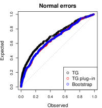
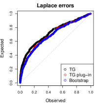
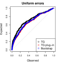
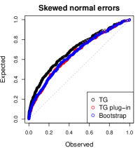
Step 2, p-values

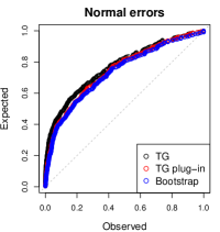
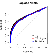
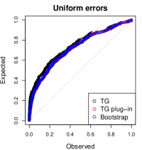
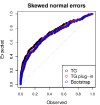
Step 3, p-values

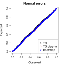
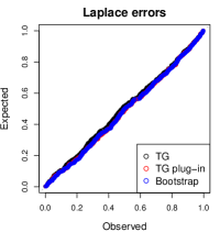
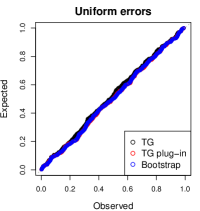
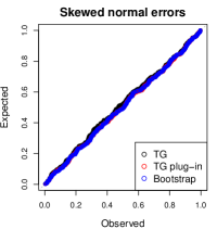
(a) P-values are shown, after each of 3 steps of LAR.

All steps, pivotal statistics

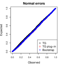
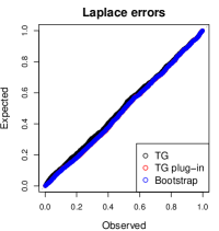
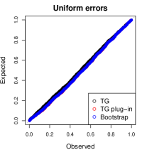
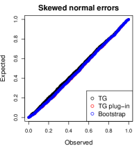
(b) Pivotal statistics are shown, aggregated over all 3 steps of LAR.

Figure 8: QQ plots as in Figure 3, but in a setup where the predictor variables have pairwise correlation 0.5.

A.13 Confidence intervals for uniform, Laplace, and skew normal noise

Figures 9 through 11 show sample confidence intervals for the problem setting of Section 6.2, when the error distribution is uniform, Laplace, and skew normal, respectively.

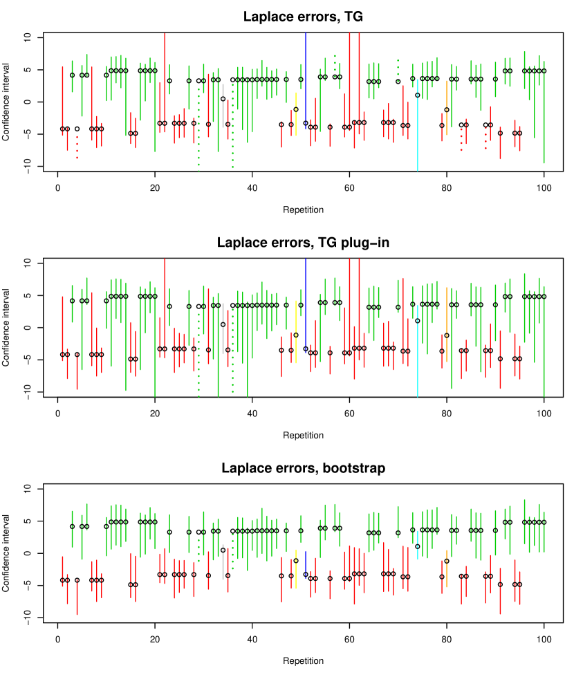
Figure 9: Confidence intervals from 100 draws of $Y$, similar to those in Figure 4, but under a uniform noise distribution.

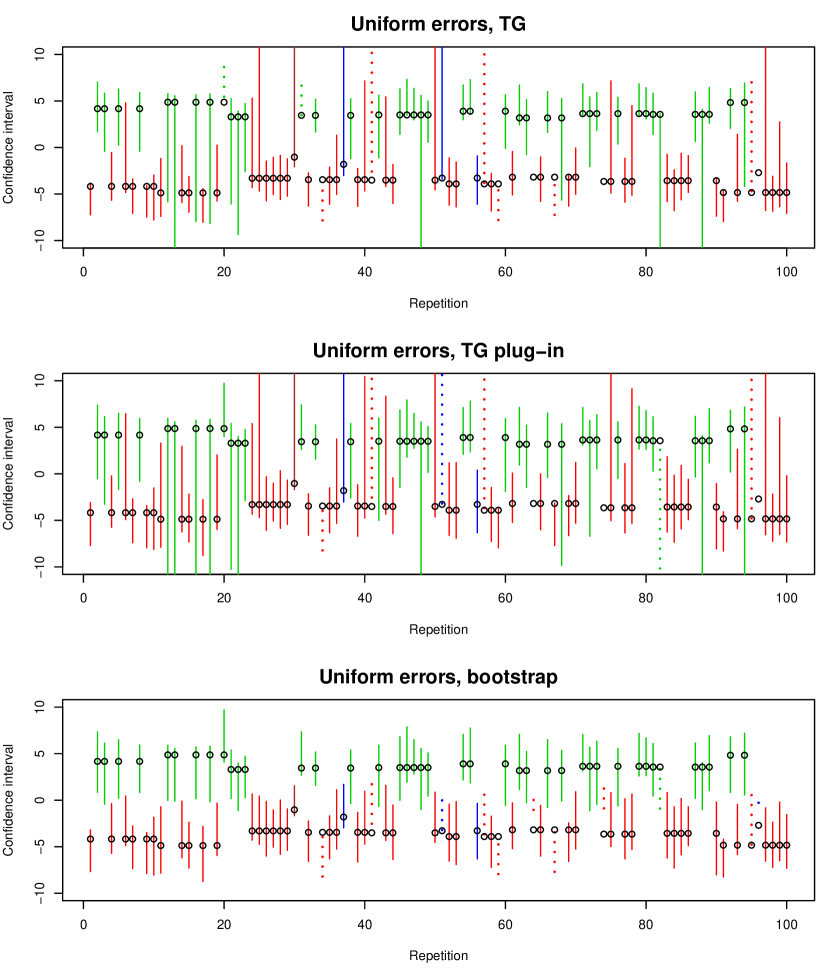
Figure 10: Confidence intervals from 100 draws of $Y$, similar to those in Figure 4, but under a Laplace noise distribution.

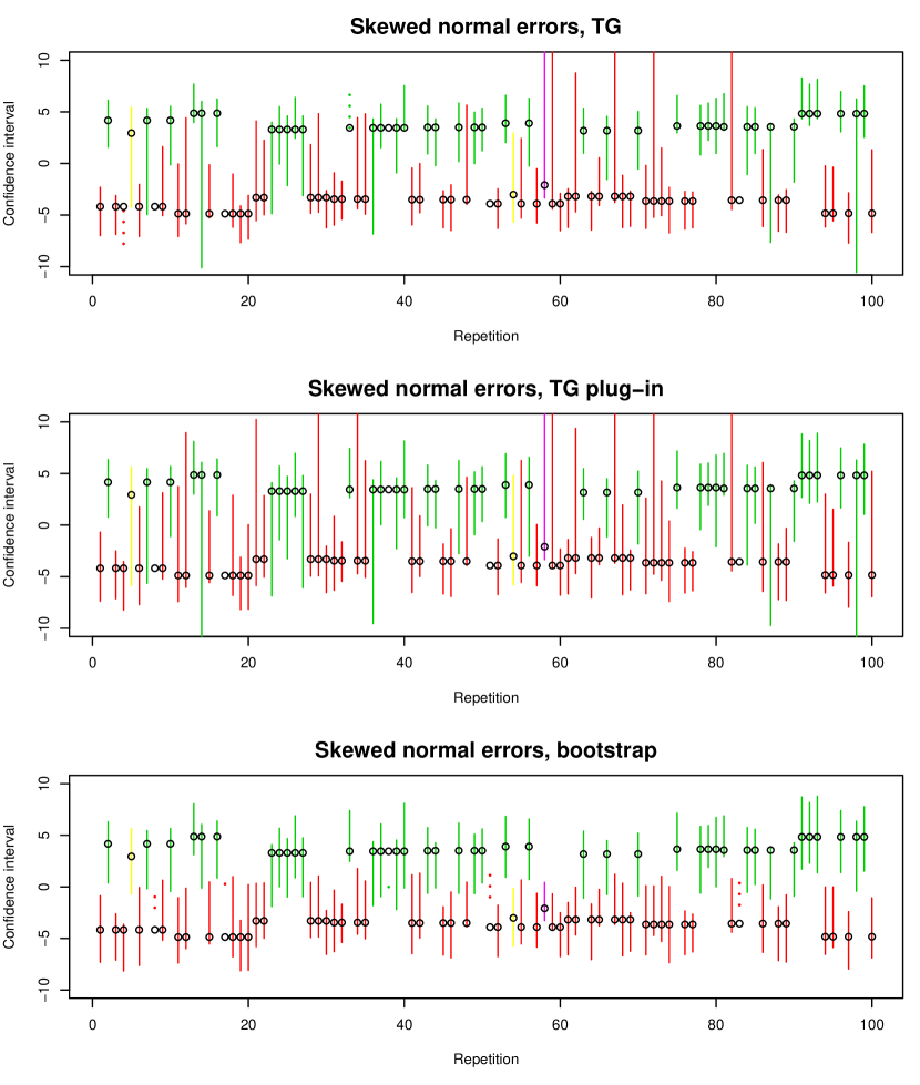
Figure 11: Confidence intervals from 100 draws of $Y$, similar to those in Figure 4, but under a skew normal noise distribution.

A.14 Confidence interval summary statistics for correlated predictors

Table 2 gives summary statistics of confidence intervals obtained by inverting the original TG, plug-in TG, and bootstrap TG statistics, as in Table 1 of Section 6.2, but for the correlated predictors setup described in Section A.12.

N	TG
	Plug-in
	Boot
L	TG
	Plug-in
	Boot
U	TG
	Plug-in
	Boot
S	TG
	Plug-in
	Boot

Step 1
Coverage	Power	Width
0.908	0.220	6.907
0.926	0.186	8.186
0.924	0.192	4.973
0.912	0.264	6.510
0.928	0.182	7.341
0.934	0.176	5.117
0.910	0.226	6.826
0.926	0.154	8.192
0.918	0.172	4.949
0.904	0.240	6.479
0.912	0.174	7.717
0.908	0.192	4.973

Step 2
Coverage	Power	Width
0.920	0.244	25.960
0.922	0.210	30.113
0.916	0.254	8.745
0.886	0.290	23.668
0.894	0.264	26.841
0.916	0.294	8.769
0.898	0.262	25.371
0.906	0.200	29.211
0.886	0.280	8.817
0.910	0.262	24.502
0.920	0.218	28.979
0.904	0.254	8.697

Step 3
Coverage	Power	Width
0.904	0.110	55.614
0.908	0.106	66.083
0.914	0.116	10.667
0.894	0.126	54.351
0.894	0.130	60.831
0.884	0.148	10.583
0.920	0.106	52.786
0.922	0.098	63.915
0.910	0.122	10.474
0.892	0.136	56.700
0.894	0.120	68.143
0.896	0.122	10.486

Table 2: Summary statistics for 90% confidence intervals, as in Table 1, but in a modified problem setting such that the predictor variables have pairwise correlation 0.5. The standard errors are roughly 0.01, 0.02, and 0.87 for the coverage, power, and width statistics, respectively.

A.15 Proof of Theorem 12

Let us denote by $N_{j}$ the number of observations in the $j$th column of the data array $Y_{ij}$, $i=1,\ldots,m$, $j=1,\ldots,d$ that are drawn from the $N(B,1)$ mixture component. Similarly, let $N^{\prime}_{j}$ denote the number of observations in the $j$th column drawn from the $N(0,1)$ mixture component. Then we will define $E$ to be the event

$$E=\Big{\{}\text{For some $j=1,\ldots,d$, we have $N_{j}=m$ and $N^{\prime}_{\ell}\geq m-2\pi md$ for all $\ell\not=j$}\Big{\}}.$$

In words, $E$ is the event that exactly one column has all of its observations drawn from $N(B,1)$, and each of the rest of the $d-1$ columns have at least $m-2\pi md$ observations from $N(0,1)$. We calculate

$$\mathbb{P}(E) =d\pi^{m}\mathbb{P}\big{(}N^{\prime}_{1}\geq m-2\pi md\big{)}^{d-1}$$

$$=\Big{(}1-\mathbb{P}\big{(}N^{\prime}_{1}+\widetilde{N}_{1}\geq 2\pi md\big{)}\Big{)}^{d-1}$$

$$\geq\Bigg{(}1-\frac{1}{d}\Bigg{)}^{d-1}$$

$$\to 1/e,$$

where in the second line we used that $d\pi^{m}=1$ by construction, and introduced the notation $\widetilde{N}_{j}$ for the number of observations in column $j$ that are drawn from the $N(-B,1)$ mixture component; in the third line we used Markov’s inequality.

On the event $E$, intersected with an event whose probability tends to one, we have $W_{(1)},W_{(2)}\to\infty$, and furthermore

$$\sqrt{m}W_{(1)} \geq\sqrt{m}B+Z_{0}\geq\sqrt{m}B/2,$$

$$\sqrt{m}W_{(2)} \leq 2\pi m^{3/2}dB+\max_{j=1,\ldots,d-1}\;Z_{j}\leq 4\pi m^{3/2}dB,$$

where $Z_{0},Z_{1},\ldots,Z_{d-1}$ denote standard normals. We note that the ultimate bounds on the right-hand sides in the two lines above are extremely loose, but will suffice for our purposes. Hence using Mills’ ratio, we can bound the TG statistic on the event in consideration by

$$\pazocal{T}(Y;0) \leq\exp\Bigg{(}-\frac{\big{(}mW_{(1)}^{2}-mW_{(2)}^{2}\big{)}}{4}\Bigg{)}\frac{W_{(2)}}{W_{(1)}}\Bigg{(}1+\frac{2}{mW_{(2)}^{2}}\Bigg{)}$$

$$\leq 2\exp\Bigg{(}-\frac{\big{(}mW_{(1)}^{2}-mW_{(2)}^{2}\big{)}}{4}\Bigg{)},$$

for sufficiently large $d$. But on this same event we have that

$$mW_{(1)}^{2}-mW_{(2)}^{2}\geq mB^{2}\Bigg{(}\frac{1}{4}-16\pi^{2}m^{2}d^{2}\Bigg{)},$$

and it is straightforward to check that the right-hand side of the bound above diverges to $\infty$, given our assumptions on $m,d,\pi,B$. Therefore, we have shown that on an event whose probability tends to at least $1/e$, the TG statistic converges to 0.

As for the conditional result, notice that for any model $(j,s)$, we have by symmetry (under $\mu=0$) $\mathbb{P}(T(Y;j,s,0)\leq t\,|\,\widehat{M}(Y)=(j,s))=\mathbb{P}(\pazocal{T}(Y;0)\leq t)$, as well as $\mathbb{P}(E\,|\,\widehat{M}(Y)=(j,s))=\mathbb{P}(E)$. Hence the conditional TG statistic $T(Y;j,s,0)\,|\,\widehat{M}(Y)=(j,s)$ itself cannot be asymptotically uniform, and converges to 0 on a event whose limiting probability is at least $1/e$, conditional on $\widehat{M}(Y)=(j,s)$.

A.16 Some thoughts on instability in high dimensions

The TG statistic is defined by the ratio of normal tail probabilities. If the dimension $d$ is large (in which case we are searching through a large space of models), or there are some large effects, then we often find ourselves evaluating the pivot far into the tails. The point of evaluation is given by a linear function of the data, which should itself converge to a Gaussian distribution (at least when $d$ is finite). But even a small amount of non-Gaussianity is magnified when we are in the tails. To see this, consider the function

$$H_{p}(t)=\frac{\int_{t+1}^{\infty}p(z)\,dz}{\int_{t}^{\infty}p(z)\,dz}.$$

The left plot in Figure 12 shows two densities $p$ and $q$ which are nearly indistinguishable. The right plot shows their corresponding tail functions $H_{p}$ and $H_{q}$. Even though $p$ and $q$ are close, we see that $H_{p}$ and $H_{q}$ are quite different. The message is that any inferential method that depends heavily on extreme tail behavior could be unreliable.

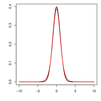
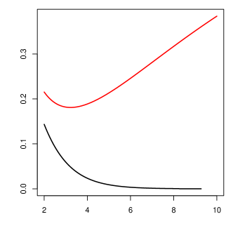
Figure 12: The left plot shows two densities $p,q$, in black and red; the right shows their tail functions $H_{p},H_{q}$ (in corresponding colors).

Perhaps more visually striking is a plot of the TG statistic, when viewed as a function of $y$ (for $X$ fixed). This is shown in Figure 13, where the statistic is used to test $\mu=0$, and we used the same setup—thus the same model selection partition elements, and even matching colors—as in Figure 2. Here $n=2$, so it is possible to fully visualize the TG statistic as a function of $y\in\mathbb{R}^{2}$. This function is not well-behaved at the boundaries between partition elements corresponding to different model selection events. Technically, this function is continuous on the interior of each partition element, which permits an application of the (uniform) continuous mapping theorem when $d$ is fixed. But the derivatives at the boundaries are infinite and, especially in high-dimensional problem settings, there is a nonnegligible probability of being near a boundary. Thus a small perturbation to the data could have a dramatic effect on the value of the pivot.

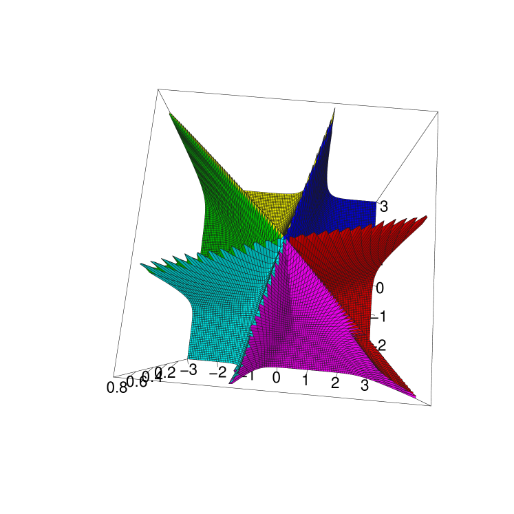
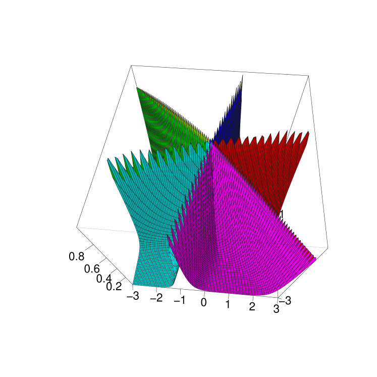
Figure 13: Two 3d views of the TG statistic, with the pivot value set at $\mu=0$, in same setup as in Figure 2. Here $n=2$, and the statistic is plotted as a function of $y\in\mathbb{R}^{2}$.

References

- (1)
- Bachoc et al. (2014) Bachoc, F., Leeb, H. & Potscher, B. (2014), Valid confidence intervals for post-model-selection predictors. arXiv: 1412.4605.
- Berk et al. (2013) Berk, R., Brown, L., Buja, A., Zhang, K. & Zhao, L. (2013), ‘Valid post-selection inference’, Annals of Statistics 41(2), 802–837.
- Chen et al. (2011) Chen, L., Goldstein, L. & Shao, Q.-M. (2011), Normal Approximation by Stein’s Method, Springer.
- Choi et al. (2014) Choi, Y., Taylor, J. & Tibshirani, R. (2014), Selecting the number of principal components: estimation of the true rank of a noisy matrix. arXiv: 1410.8260.
- Donoho (1988) Donoho, D. (1988), ‘One-sided inference about functionals of a density’, Annals of Statistics 16(4), 1390–1420.
- Fithian et al. (2014) Fithian, W., Sun, D. & Taylor, J. (2014), Optimal inference after model selection. arXv: 1410.2597.
- Hyun et al. (2016) Hyun, S., G’Sell, M. & Tibshirani, R. J. (2016), Exact post-selection inference for changepoint detection and other generalized lasso problems. arXv: 1606.03552.
- Kasy (2015) Kasy, M. (2015), Uniformity and the delta method. Unpublished manuscript.
- Lee et al. (2016) Lee, J., Sun, D., Sun, Y. & Taylor, J. (2016), ‘Exact post-selection inference, with application to the lasso’, Annals of Statistics 44(3), 907–927.
- Lee & Taylor (2014) Lee, J. & Taylor, J. (2014), ‘Exact post model selection inference for marginal screening’, Advances in Neural Information Processing Systems 27, 136–144.
- Leeb & Potscher (2003) Leeb, H. & Potscher, B. (2003), ‘The finite-sample distribution of post-model-selection estimators and uniform versus nonuniform approximations’, Econometric Theory 19(1), 100–142.
- Leeb & Potscher (2006) Leeb, H. & Potscher, B. (2006), ‘Can one estimate the conditional distribution of post-model-selection estimators?’, Annals of Statistics 34(5), 2554–2591.
- Leeb & Potscher (2008) Leeb, H. & Potscher, B. (2008), ‘Can one estimate the unconditional distribution of post-model-selection estimators?’, Econometric Theory 24(2), 338–376.
- Lockhart et al. (2014) Lockhart, R., Taylor, J., Tibshirani, R. J. & Tibshirani, R. (2014), ‘A significance test for the lasso’, Annals of Statistics 42(2), 413–468.
- Loftus & Taylor (2014) Loftus, J. & Taylor, J. (2014), A significance test for forward stepwise model selection. arXiv: 1405.3920.
- O’Hagan & Leonard (1976) O’Hagan, A. & Leonard, T. (1976), ‘Bayes estimation subject to uncertainty about parameter constraints’, Biometrika 63(1), 201–203.
- Reid et al. (2017) Reid, S., Taylor, J. & Tibshirani, R. (2017), ‘Post-selection point and interval estimation of signal sizes in Gaussian samples’, Canadian Journal of Statisitcs 45(2), 128–148.
- Rosenthal (1970) Rosenthal, H. (1970), ‘On the subspaces of () spanned by sequences of independent random variables’, Israel Journal of Mathematics 8(3), 273–303.
- Taylor et al. (2016) Taylor, J., Loftus, J. & Tibshirani, R. J. (2016), ‘Inference in adaptive regression via the kac-rice formula’, Annals of Statistics 44(2), 743–770.
- Tian & Taylor (2017) Tian, X. & Taylor, J. (2017), ‘Asymptotics of selective inference’, Scandinavian Journal of Statistics 44(2), 480–499.
- Tibshirani et al. (2016) Tibshirani, R. J., Taylor, J., Lockhart, R., & Tibshirani, R. (2016), ‘Exact post-selection inference for sequential regression procedures’, Journal of the American Statistical Association 111(514), 600–620.
- van der Vaart (1998) van der Vaart, A. (1998), Asymptotic Statistics, Cambridge University Press.
- Wasserman (2014) Wasserman, L. (2014), ‘Discussion: A significance test for the lasso’, Annals of Statistics 42(2), 501–508.