Categorical Data Fusion Using Auxiliary Information

Abstract

In data fusion analysts seek to combine information from two databases comprised of disjoint sets of individuals, in which some variables appear in both databases and other variables appear in only one database. Most data fusion techniques rely on variants of conditional independence assumptions. When inappropriate, these assumptions can result in unreliable inferences. We propose a data fusion technique that allows analysts to easily incorporate auxiliary information on the dependence structure of variables not observed jointly; we refer to this auxiliary information as glue. With this technique, we fuse two marketing surveys from the book publisher HarperCollins using glue from the online, rapid-response polling company CivicScience. The fused data enable estimation of associations between people’s preferences for authors and for learning about new books. The analysis also serves as a case study on the potential for using online surveys to aid data fusion.

KEY WORDS: imputation; integration; latent class; matching

1 Introduction

In many applications in marketing, analysts seek to combine information from two or more databases containing information on disjoint sets of individuals and distinct sets of variables (Kamakura and Wedel,, 1997; van der Putten et al.,, 2002; Kamakura et al.,, 2003; Gilula et al.,, 2006; van Hattum and Hoijtink,, 2008). For example, a company has one database on customers’ purchasing habits and another database on individuals’ media viewing habits, and seeks to find associations between viewing and purchasing habits (Gilula et al.,, 2006). This setting, known as data fusion (Rässler,, 2002, p. 60 – 63), arises in other contexts, including microsimulation modeling in economics (Moriarty and Scheuren,, 2003) and government statistics (D’Orazio et al.,, 2002). For applications in other areas, see Kadane, (2001, reprinted from a 1978 manuscript), Rodgers, (1994), Moriarty and Scheuren, (2001), and D’Orazio et al., (2006).

Typical applications of data fusion rely on strong and unverifiable assumptions about the relationships among the variables. To see this, consider fusion of two databases, $D_{1}$ and $D_{2}$, with disjoint sets of individuals. Let $A$ denote the set of variables common to both databases, such as demographics; let $B$ denote the set of variables unique to $D_{1}$; and let $B^{\prime}$ denote the set of variables unique to $D_{2}$. Since $\{A,B,B^{\prime}\}$ are never observed simultaneously, the joint distribution of $\{A,B,B^{\prime}\}$ is not identifiable based on $(D_{1},D_{2})$ alone. Neither is the distribution of $\{B,B^{\prime}\}$, either marginally or conditionally on $A$. Put another way, many possible specifications of the joint distributions of $\{A,B,B^{\prime}\}$ may be consistent with the marginal distributions of $\{A,B\}$ in $D_{1}$ and $\{A,B^{\prime}\}$ in $D_{2}$. The data provide no information on which specifications to favor.

For data fusion to proceed, analysts must make some assumption about the joint distribution of $\{A,B,B^{\prime}\}$. The most common assumption is that the variables in $B$ are conditionally independent of those in $B^{\prime}$, given the variables in $A$ (Kiesl and Rässler,, 2006; D’Orazio et al.,, 2006; Gilula et al.,, 2006). For example, assume that every person with the same age, gender, occupation, race, county of residence, etc., has the same probability of purchasing the product, regardless of their media viewing habits. While this assumption could be reasonable in some contexts with rich $A$ variables, it also could be grossly incorrect. For example, in some demographic groups, people who watch advertising infrequently may be less likely to purchase the product. When this is the case, assuming conditional independence can result in inferences about $\{A,B,B^{\prime}\}$ that do not accurately reflect the underlying relationships in the population.

To reduce reliance on conditional independence assumptions, analysts require some form of auxiliary information. For example, analysts can use knowledge about the joint distribution of $\{B,B^{\prime}\}$ from other sources to bound the joint distribution of $\{A,B,B^{\prime}\}$ (D’Orazio et al.,, 2006). Another possibility is to mount a new data collection that provides information on unknown features of the joint distribution of $\{A,B,B^{\prime}\}$. Historically, such surveys have been untimely and prohibitively expensive. However, in recent years technological advances have opened the door to fielding rapid response, low cost surveys (Gilula and McCulloch,, 2013). Questions then arise as to how analysts can leverage the information in such surveys for more accurate data fusion.

In this article, we propose a data fusion approach that allows analysts to incorporate auxiliary information on arbitrary subsets of $\{A,B,B^{\prime}\}$ with at least one variable in $B$ and $B^{\prime}$ jointly observed. We refer to such auxiliary information as glue, since it serves to strengthen the connection between $B$ and $B^{\prime}$. We present the approach for the common setting of all categorical variables, although similar strategies could be used for numerical variables. The basic idea is to collect or construct a dataset that represents the auxiliary information, append this dataset to the concatenated file $(D_{1},D_{2})$, and fit an imputation model to predict missing $B$ in $D_{2}$ and missing $B^{\prime}$ in $D_{1}$. As the engine for imputation, we use a Bayesian latent class model (Dunson and Xing,, 2009; Si and Reiter,, 2013). Using simulation studies, we illustrate how to accommodate glue of various sizes and on various variable subsets, and demonstrate the potential for glue to improve accuracy relative to fusion procedures that assume conditional independence. We also discuss problems that can arise when using glue from a non-representative sample, and propose methodology for incorporating non-representative glue in data fusion. We apply the methodology in a data fusion experiment in which we obtain glue from the internet polling company CivicScience, and use the glue to fuse surveys fielded by the book publisher HarperCollins Publishers on author preferences and author discovery tendencies.

The remainder of the article is organized as follows. In Section 2, we introduce the HarperCollins data fusion context and review typical approaches to data fusion in the literature. In Section 3, we describe how to adapt Bayesian latent class models for data fusion to accommodate glue. The approach allows for both the creation of completed data files, i.e., as in multiple imputation (Rubin,, 1986, 1987; Reiter,, 2012), as well as parameter inference. We focus on creating completed datasets, which can be subsequently analyzed using the techniques of Rubin, (1987). We also summarize results of simulation studies that demonstrate the benefits of leveraging glue in data fusion. In Section 4, we present results of the HarperCollins Publishers’ and CivicScience data fusion. In Section 5, we conclude with a discussion of open questions and future research directions.

2 Background

2.1 HarperCollins data and CivicScience glue

HarperCollins Publishers routinely administers surveys to the public to learn about their behaviors and opinions, relying on this information to guide business decisions. The surveys typically include questions about basic demographics (e.g., age, income, gender) and reading habits, as well as questions on focused topics such as technology usage or author preferences. Generally, around 10% of questions in the surveys address basic demographics and reading habits, and the remaining 90% are specific to the survey. We seek to fuse data from two HarperCollins surveys, one including questions on the authors people read and the other including questions on where people discover new authors (e.g., Facebook and Best Sellers lists). The first survey comprises $4,001$ respondents and $734$ variables; we use only a subset of questions related to discovery and demographics. The second survey comprises $5,015$ respondents and $1,433$ variables; we use only a subset of questions related to author readership and demographics. The surveys were administered by an independent company to a random sample of people residing in the United States, with pre-specified numbers of individuals in specific categories based on age, gender, ethnicity, and geographic regions.

HarperCollins is interested in understanding the demographics of readers of particular authors and how to reach them. For example, if HarperCollins publishes a new book by the author Lisa Kleypas, will they reach more of her readers by advertising the new book in bookstores or on Facebook? Furthermore, who should be the target audience (age, gender, etc.) of the advertisements? Leveraging the connections between author readership, book discovery, and demographics across surveys can help HarperCollins pursue profitable marketing strategies.

To obtain glue for the data fusion, we collaborated with internet polling company CivicScience. Internet polling companies are potentially ideal glue collectors, as they are able to survey thousands of people daily at low cost. As case in point, CivicScience collects hundreds of thousands of responses per day and has information stored on millions of respondents. CivicScience is routinely paid by other companies to canvass the public on marketing and business decisions.

CivicScience obtains information by posting short surveys, typically three or four questions, on the sidebar of popular websites. Participation is purely voluntary (raising the potential for selection bias, which we return to later). CivicScience entices participation by beginning each survey with an engagement question that people are often willing and eager to share their opinion on (e.g., “Who will win the Superbowl?”). The next question(s) is a value question asked on behalf of a paying client. The final question inquires about respondent demographics. After completing the short survey, participants are offered the option to answer additional questions. CivicScience uses participants’ computer IP addresses to link responses from the same individuals (more accurately, from the same computer).

For our application, CivicScience ran numerous three-question surveys on author readership and discovery. The second question was about either author readership or discovery, and the third question was about either the respondent’s age or gender. Many participants completed more than one survey, allowing CivicScience to link responses on author readership, discovery, age, and gender. We use these linked data in the fusion of the HarperCollins surveys.

2.2 Common data fusion methods

The most widely used data fusion technique in practice is statistical matching (van der Putten et al.,, 2002; Wicken and Elms,, 2009). The analyst divides the observations in $(D_{1},D_{2})$ into groups based on the similarity of values in the $A$ variables. Within each group, the analyst imputes missing $B$ values for records in $D_{2}$ by sampling from the empirical distribution of $B^{\prime}$ in that group. The analyst imputes missing $B^{\prime}$ values for records in $D_{1}$ in a similar manner. Often one cannot find groups of records in $D_{1}$ and $D_{2}$ with exactly the same values on all of $A$, particularly when the contingency table implied by the variables in $A$ has a large number of cells. In such cases, analysts form groups based on some subset of $A$ variables. Alternatively, analysts specify some distance function that quantifies how “close” the $A$ values are for a given pair of observations from $D_{1}$ and $D_{2}$, and form groups based on the close matches. Regardless of how the analyst forms groups, these approaches all make the unverifiable assumption that $B$ is independent of $B^{\prime}$ within the analyst-specified groups.

A second approach to data fusion is to estimate regression models for the distributions of $(B\mid A)$ from $D_{1}$ and $(B^{\prime}\mid A)$ from $D_{2}$, and set $f(B,B^{\prime}\mid A)=f(B\mid A)f(B^{\prime}\mid A)$, i.e., assume conditional independence between $B$ and $B^{\prime}$ (Rodgers,, 1994; Gilula et al.,, 2006). One then imputes missing values of $B$ using the estimated model for $(B\mid A)$, and imputes missing values of $B^{\prime}$ using the estimated model for $(B^{\prime}\mid A)$. Gilula et al., (2006) describe how to adapt this regression-based approach to incorporate auxiliary information about the dependence between a single binary $B$ and a single binary $B^{\prime}$.

A third approach is to estimate models for the entire joint distribution of $\{A,B,B^{\prime}\}$. For example, one could use a multinomial distribution with probabilities constrained by a log-linear model that excludes terms involving interactions between $B$ and $B^{\prime}$. This also assumes conditional independence between $B$ and $B^{\prime}$. D’Orazio et al., (2006) describe how this conditional independence assumption can be relaxed in log-linear models by incorporating auxiliary information on marginal probabilities for $(B,B^{\prime})$. Alternatively, one could estimate the joint distribution of $\{A,B,B^{\prime}\}$ with a latent class model (Goodman,, 1974), as suggested by Kamakura and Wedel, (1997) and as we do here. Unlike log-linear models, latent class models can capture complex associations among the variables automatically, avoiding the difficult task of deciding which interactions to include from the enormous space of possible models (Vermunt et al.,, 2008; Si and Reiter,, 2013). Latent class models also easily handle missing values in $D_{1}$ and $D_{2}$ due to item nonresponse within the surveys, assuming nonresponse is missing at random (Rubin,, 1976). However, we are not aware of methodology for incorporating auxiliary information when using latent class models in data fusion. We now introduce such methodology.

3 Methodology

3.1 Bayesian latent class models for categorical data fusion

Suppose that we seek to fuse database $D_{1}$ comprising $n_{1}$ individuals with database $D_{2}$ comprising $n_{2}$ individuals. Let $Y_{ij}\in\{1,\dots,d_{j}\}$ be the value of variable $j$ for individual $i$, where $j=1,\dots,p$ and $i=1,\dots,n_{1}+n_{2}$. Let $Y_{i}=(Y_{i1},\dots,Y_{ip})$ for all $i$. The $p$ variables form a contingency table with $\prod_{j=1}^{p}d_{j}$ cells. For variables $j\in A$, we observe $Y_{ij}$ for all $n=n_{1}+n_{2}$ individuals; for variables $j\in B$, we observe $Y_{ij}$ for only the $n_{1}$ individuals in $D_{1}$; and, for variables $j\in B^{\prime}$, we observe $Y_{ij}$ for only the $n_{2}$ individuals in $D_{2}$. We note that, in practice, item nonresponse will result in unintentionally missing values within $D_{1}$ and $D_{2}$ as well.

In latent class models for categorical data, we assume that each individual is a member of one of $N$ unobserved classes. Let $Z_{i}\in\{1,\dots,N\}$ denote individual $i$’s class membership, and let $\pi_{l}=\mathrm{P}(Z_{i}=l)$ be the probability that individual $i$ is in class $l$. We assume that $\pi=(\pi_{1},\dots,\pi_{N})$ is the same for all individuals. Within each class, we assume the variables follow independent categorical distributions with variable-specific probabilities $\phi_{l}^{(j)}=(\phi_{l1}^{(j)},\dots,\phi_{ld_{j}}^{(j)})$, where $\phi_{ly}^{(j)}=\mathrm{P}(Y_{ij}=y\mid Z_{i}=l)$. As a flexible and computationally convenient prior distribution on $\pi$ and $\{\phi_{l}^{(j)}\}$, we use the truncated version of the Dirichlet Process (DP) prior (Sethuraman,, 1994). The complete model, referred to as the DP mixture of products of multinomials (DPMPM), can be expressed as:

$$Y_{i1},\dots,Y_{ip}|Z_{i},\phi \stackrel{{\scriptstyle ind.}}{{\sim}}\prod_{j=1}^{p}\mathrm{categorical}(Y_{ij};\phi_{z_{i}1}^{(j)},\dots,\phi_{z_{i}d_{j}}^{(j)}),\quad i=1,\dots,n$$ (1)

$$Z_{i}\mid\pi \stackrel{{\scriptstyle ind.}}{{\sim}}\mathrm{categorical}(\pi_{1},\dots,\pi_{N}),\quad i=1,\dots,n$$ (2)

$$\pi_{l} =V_{l}\prod_{r=1}^{l-1}(1-V_{r}),\,\,\,\pi_{N}=1-\sum_{l=1}^{N-1}\pi_{l}$$

$$V_{l}\mid\alpha \stackrel{{\scriptstyle iid}}{{\sim}}\mathrm{beta}(1,\alpha),\,\,V_{N}=1,\quad l=1,\dots,N-1$$

$$\phi_{l}^{(j)} \stackrel{{\scriptstyle ind.}}{{\sim}}\mathrm{Dir}(a_{1}^{(j)},\dots,a_{d_{j}}^{(j)}),\quad l=1,\dots,N,\>j=1,\dots,p$$

$$\alpha \sim\mathrm{gamma}(a_{\alpha},b_{\alpha}).$$ (3)

The parameter $\alpha$ plays a central role in determining the number of effective components in the mixture, with smaller values favoring fewer components. A hyperprior on $\alpha$ allows the data to inform the number of components. In our applications, we fix $a_{\alpha}$ and $b_{\alpha}$ equal to $0.5$ in the prior distribution in (3), which represents a relatively noninformative prior. We set $a_{1}^{(j)}=\dots=a_{d_{j}}^{(j)}=1$ for all $j$.

We estimate the DPMPM model using Markov chain Monte Carlo (MCMC) posterior simulation techniques (Ishwaran and Zarepour,, 2000; Ishwaran and James,, 2001). The missing $Y_{ij}$, unforeseen from item nonresponse and expected due to the the structure of data fusion, are imputed as part of the MCMC. Given a draw of model parameters $(\alpha,\{\phi^{(j)}\},Z,V,\pi)$, we sample a value for each missing $Y_{ij}$ from the relevant independent categorical distribution in class $Z_{i}$. Further details on the sampling algorithm are provided in the Appendix.

The probability model defined in (1) and (2) is the same as that used by Kamakura and Wedel, (1997). However, rather than use a fully Bayesian estimation approach, they maximize the likelihood function obtained from equations (1) and (2). Additionally, Kamakura and Wedel, (1997) use heuristics to determine some optimal number of classes, whereas with the DPMPM one simply can fix the truncation level $N$ to a large value (Ishwaran and James,, 2001). To ensure that $N$ is large enough, the analyst confirms that the number of occupied classes $n^{*}$ is always significantly less than $N$ across MCMC samples. If the posterior distribution for $n^{*}$ places significant mass near $N$, then $N$ should be increased. In the analyses in this article, $N=30$ is always sufficiently large.

Even though variables are independent within the latent classes, variables still can be marginally dependent across the set of classes. For example, for any pair of variables $j$ and $j^{\prime}$, we have

$$P(Y_{ij}=y,Y_{ij^{\prime}}=y^{\prime}\mid\pi,\{\phi^{(j)}\})=\sum_{l=1}^{N}\pi_{l}\phi_{l,y}^{(j)}\phi_{l,y^{\prime}}^{(j^{\prime})}.$$ (4)

In general, the expression in (4) is not identical to the product of the two marginal probabilities, $\left(\sum_{l=1}^{N}\pi_{l}\phi_{l,y}^{(j)}\right)\left(\sum_{l=1}^{N}\pi_{l}\phi_{l,y^{\prime}}^{(j^{\prime})}\right)$, implying $Y_{ij}$ and $Y_{ij^{\prime}}$ are independent conditional on $Z_{i}$ and $\{\phi^{(j)}\}$, but dependent upon marginalization over $Z_{i}$. Expression (4) can be used for model-based inferences about probabilities.

As suggested by Gilula et al., (2006) when discussing the model used by Kamakura and Wedel, (1997), estimates of the joint distribution of $\{A,B,B^{\prime}\}$ from latent class models may not be concordant with conditional independence. In our simulations, we found that the DPMPM favors somewhat stronger correlation between $B$ and $B^{\prime}$ than is implied under conditional independence. This results from the clustering engendered by the DP prior specification, since the data contain no information about $\{B,B^{\prime}\}$ jointly. This finding underscores the potential benefits of using glue when using latent class models for data fusion.

3.2 Incorporating glue in data fusion

Schifeling and Reiter, (2015) developed a strategy for incorporating prior information about marginal probabilities into the DPMPM. They suggest constructing a hypothetical dataset that represents prior beliefs, appending it to the collected data, and estimating the latent class model with the concatenated real and hypothetical data. As an example, if one knows only that the true proportion of women in a population is exactly 50%, one can append a large hypothetical dataset with equal numbers of men and women with all other variables missing. Schifeling and Reiter, (2015) show that this approach fixes the posterior probability of being female at 50% without distorting the conditional distributions of other variables on gender.

We adapt this strategy to incorporate glue in data fusion. We assume that the analyst has glue data, $D_{s}$, in which some subset of the $\{B,B^{\prime}\}$ variables, possibly with $A$, is measured. For individuals $i=1,\dots,n_{s}$ in $D_{s}$, let $Y_{i}$ be the $p\times 1$ vector of measurements for the $i$th individual. In most data fusion scenarios, each $Y_{i}$ will be incomplete by design, in that only some variables are available in $D_{s}$. We assume that $Y_{i}$ for individuals in $D_{s}$ follows the model in (1) – (3). Thus, we concatenate $(D_{1},D_{2},D_{s})$ in one file, and estimate the DPMPM model using MCMC. The information on $\{A,B,B^{\prime}\}$ available in $D_{s}$ influences the parameter estimates, resulting in imputations of missing $B$ variables in $D_{2}$ and $B^{\prime}$ variables in $D_{1}$ that reflect the dependence relationships in the glue. For computational convenience, when fitting the MCMC we impute missing values in $D_{1}$ and $D_{2}$, but not those in $D_{s}$.

The ideal glue includes data on all variables in $(A,B,B^{\prime})$ and is a sample from the distribution of $(A,B,B^{\prime})$ in the population of interest. In practice, glue may be available only on subsets of variables, such as $(B,B^{\prime})$. In addition, $D_{s}$ may not be representative of the population. For example, in the HarperCollins and CivicScience data fusion, only the conditional distributions $P(B\mid A,B^{\prime})$ can be plausibly considered representative.

To investigate the potential benefits of glue in these scenarios, we use three sets of simulation studies. First, we add glue on different subsets of variables to explore the intuition that richer glue (i.e., glue that contains more variables simultaneously observed) results in larger improvements in inference. Second, we analyze the sensitivity of inference to the addition of varying amounts of data subjects in the glue. Third, we study the validity of inferences when using glue that is not representative of the population distribution of $(A,B,B^{\prime})$. We also present a method for appropriately incorporating such information. We note that each of these issues arises when using the CivicScience data as glue.

3.3 Simulation studies with representative glue

We simulate fusion settings using a third HarperCollins survey containing $4,000$ respondents and $1,056$ variables. As the $A$ variables, we select demographics including gender, age, work status, and income. As the $B$ and $B^{\prime}$ variables, we select eBook reader ownership and number of hours spent reading per week, respectively. Table 1 describes the variables in detail. We create $D_{1}$ by randomly selecting half of the $3,567$ complete cases and removing reading hours, and create $D_{2}$ as the remaining half of the complete case data with eBook reader ownership removed. We are interested in fusing $D_{1}$ and $D_{2}$ to estimate the relationship between eBook reader ownership and reading hours per week, conditional on specific demographics variables. Because we have the complete observations of $\{A,B,B^{\prime}\}$ in the original data, we can compare results from data fusion to the ground truth.

To quantify the potential for glue in this example, we investigated the Fréchet bounds (D’Orazio et al.,, 2006) on $P(B=j,B^{\prime}=k)$ for $j=1,2$ and $k=1,2,3$, as implied by the marginal distributions $P(A,B)$ and $P(A,B^{\prime})$. If these bounds are tight, signifying the probabilities are highly constrained by the observed marginal probabilities $P(A,B)$ and $P(A,B^{\prime})$, then little is to be gained from incorporating glue. Conversely, if the bounds on the cell probabilities of $P(B,B^{\prime})$ are wide, glue has the potential to greatly improve inferences based on $P(B,B^{\prime})$. Note that the marginal distributions $P(B)$ and $P(B^{\prime})$ themselves constrain $P(B,B^{\prime})$. The Fréchet bound widths on the six cell probabilities ranged from 0.163 to 0.169. This implies that even with observing $\{A,B\}$ and $\{A,B^{\prime}\}$ there remains a lot of uncertainty about $\{B,B^{\prime}\}$, and potentially much to be gained from collecting glue.

Table 1: Variables contained in the HarperCollins survey used for simulations.

Variable	Group	Levels (Level Label)
gender	$A$	male (1), female (2)
age	$A$	18-24 (1), 25-34 (2), 35-44 (3), 45-54 (4), 55-64 (5), 65+ (6)
work status	$A$	emp FT (1), emp PT (2), homemaker (3), retired (4), self-employed (5), other (6)
income	$A$	$<$25K (1), 25-45K (2), 45-75K (3), 75-99K (4), 100+K (5), won’t say (6)
eBook	$B$	yes (1), no (2)
hours	$B^{\prime}$	$<1$ (1), 1-4 (2), 5+ (3)

3.3.1 Glue richness

We consider four types of glue for $D_{s}$. In increasing order of richness, these include only the marginal distribution $\{B,B^{\prime}\}$, the joint distribution of $\{A_{g},B,B^{\prime}\}$ where $A_{g}$ represents gender, the joint distribution of $\{A_{a},B,B^{\prime}\}$ where $A_{a}$ represents age, and the joint distribution of $\{A_{g},A_{a},B,B^{\prime}\}$. In each case, we create glue by duplicating the appropriate variables for all respondents in the original survey; thus, $n_{s}=3567$. We run the MCMC chains long enough to obtain $120,000$ posterior samples of all parameters. From these runs, we sample $m=50$ completed datasets, $(D_{1}^{*},D_{2}^{*})$, which we use in multiple imputation inferences.

To evaluate the impact of glue richness, we compare Hellinger distances, which are commonly used to quantify the similarity between two probability distributions (Pollard,, 2002; Gibbs and Su,, 2002). Hellinger distances based on $\{A,B,B^{\prime}\}$ reflect the accuracy of the entire estimated joint distribution $P(A,B,B^{\prime})$, which arguably is the most important level of validity a fusion process can achieve (Rässler,, 2004). For two discrete distributions $P$ and $Q$ taking on $k$ values with probabilities $(p_{1},\dots,p_{k})$ and $(q_{1},\dots,q_{k})$, the Hellinger distance is given by $2^{-1/2}\sqrt{\sum_{i=1}^{k}(\sqrt{p_{i}}-\sqrt{q_{i}})^{2}}$. This quantity is between zero and one, where smaller values imply more similarity between the distributions. Because the richest type of glue contains observations on $\{A_{g},A_{a},B,B^{\prime}\}$, we compute Hellinger distances between the empirical distribution of $(A_{g},A_{a},B,B^{\prime})$ based on the original complete survey and the corresponding posterior inferences. Calculations of distances based on the joint distribution $(A,B,B^{\prime})$ including all demographic variables, rather than just $(A_{g},A_{a},B,B^{\prime})$, yield similar patterns.

Table 2 displays the posterior means and $95\%$ credible intervals for the Hellinger distances between the empirical distribution of $(A_{g},A_{a},B,B^{\prime})$ and the corresponding posterior estimates. The results indicate that using glue can yield significant gains in accuracy, with increasing gains with richer glue. These results also suggest that gender offers smaller gains than age, a consequence of the fact that the distribution of $\{B,B^{\prime}\}$ is more similar across gender than age. This finding is evident in all of the evaluations that follow. Table 2 also displays results from a set of fused data files using an exact matching algorithm based on all variables in $A$. The empirical joint probability distribution is comparable to that produced from the latent class model with no glue.

We also compare the sum of the absolute differences between the counts in the true contingency table for $\{A_{g},A_{a},B,B^{\prime}\}$ based on the original complete data file and those based on imputed complete data files. These counts, when divided by two, indicate how many individuals the model places in incorrect cells of the empirical contingency table. We approximate the expected number of “misclassified” individuals in an imputed data set with the empirical average over $50$ imputed data files. Mathematically, the approximation for the expected number of misclassified individuals can be expressed

$$\mathrm{E}\left(0.5\sum_{j=1}^{\prod_{k=1}^{p}d_{k}}|n_{j}-\hat{n}_{j}|\right)\approx\frac{1}{50}\sum_{m=1}^{50}\left(0.5\sum_{j=1}^{\prod_{k=1}^{p}d_{k}}|n_{j}-\hat{n}^{(m)}_{j}|\right),$$

where $\hat{n}^{(m)}_{j}$ is the number of individuals in cell $j$ in the $m$th imputed data set and $n_{j}$ is the true number of individuals in the original complete data set. Table 3 shows similar patterns as Table 2: using glue improves over approaches that assume conditional independence, with increasing gains as the glue becomes richer. We note that adding gender information to glue already containing age does not lead to much improvement in imputation accuracy.

As a more focused evaluation, we use the completed datasets to estimate a logistic regression of eBook reader ownership on reading hours and the demographics variables. The model includes terms for all main effects for all predictors, pairwise interactions between reading hours and gender and reading hours and age, and the three way interaction among reading hours, gender, and age. Letting $A_{i}$ represent income and $A_{w}$ represent work status, the link function can be expressed as

$$\mathrm{logit}(p( B=1))=\beta_{0}+\beta^{g}1(A_{g}=2)+\sum_{k=2}^{6}\beta_{k}^{a}1(A_{a}=k)+\sum_{k=2}^{6}\beta_{k}^{w}1(A_{w}=k)$$

$$+\sum_{k=2}^{6}\beta_{k}^{i}1(A_{i}=k)+\sum_{k=2}^{3}\beta_{k}^{h}1(B^{\prime}=k)+\beta^{gh}1(A_{g}=2,B^{\prime}=3)$$

$$+\beta^{ah}1(A_{a}=6,B^{\prime}=3)+\beta^{gah}1(A_{g}=2,A_{a}=6,B^{\prime}=3).$$

We estimate the coefficients from the $50$ completed data sets using the standard multiple imputation combining rules (Rubin,, 1987). As displayed in Figure 1, 18 of the 22 regression coefficients based on the original data are contained in the 95% MI confidence intervals under the data fusion model applied with no glue. All intervals contain the original data coefficients when glue includes $\{A_{a},B,B^{\prime}\}$ as well as $\{A_{g},A_{a},B,B^{\prime}\}$. Adding glue with only $\{B,B^{\prime}\}$ improves the estimates of the main effects associated with $B^{\prime}$ (reading hours). Adding glue with at least $\{A_{a},B,B^{\prime}\}$ results in further improvements, in particular resulting in more reliable estimates of the interaction term associated with $A_{a}\times B^{\prime}$ (age $\times$ hours). Clearly, even targeted inferences can be improved by collecting glue, with generally increasing gains with richer glue.

3.3.2 Glue size

In Section 3.3.1, the glue sample size was equal to the total survey sample size, that is, $n_{s}=n=3567$. Generally, this will not be the case. To evaluate the role of glue sample size, we repeated the simulations using $\{A_{g},A_{a},B,B^{\prime}\}$ as glue with different sample sizes for $D_{s}$. As shown in Table 4, as expected, more high quality glue observations result in more accurate estimates with less uncertainty. Data fusion with $n_{s}=1784$ glue cases yields inferences that are close to the ground truth and to the inferences produced with more glue cases, suggesting that even modest amounts of glue can improve inferences.

Table 2: Posterior mean and $95\%$ credible intervals for the Hellinger distance between the true and estimated probability table for $(A_{g},A_{a},B,B^{\prime})$ under five different glue scenarios, as well as the estimate obtained from a fused data set under statistical matching. *The range of Hellinger distances across 10 perfect matchings is reported to quantify matching uncertainty.

	mean	$95\%$ CI or range*
No glue	.104	(.094,.113)
$\{B,B^{\prime}\}$	.083	(.075,.091)
$\{B,B^{\prime},A_{g}\}$	.077	(.071,.084)
$\{B,B^{\prime},A_{a}\}$	.060	(.053,.068)
$\{B,B^{\prime},A_{g},A_{a}\}$	.052	(.047,.059)
Exact matching	.100	.090 - .107

Table 3: Average number of individuals in the incorrect cell of the contingency table across the complete data sets under five different glue scenarios and under statistical matching. Ten complete data sets were considered for the statistical matching procedure.

	$\mathrm{E}\left(0.5\sum_{j=1}^{\prod_{j=1}^{p}d_{j}}|n_{j}-\hat{n}_{j}|\right)$
no glue	318.5
$\{B,B^{\prime}\}$	250.5
$\{B,B^{\prime},A_{g}\}$	247.0
$\{B,B^{\prime},A_{a}\}$	199.5
$\{B,B^{\prime},A_{g},A_{a}\}$	196.0
Exact matching	315.0

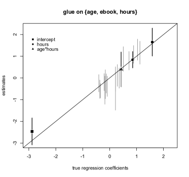
Figure 1: Point estimates and $95\%$ confidence intervals for estimated versus true regression coefficients under five different glue scenarios. The first plot refers to the no glue scenario, and highlights terms which are affected by adding glue. These same $4$ terms are highlighted in the remaining plots as more glue is added.

Table 4: Posterior mean and width of $95\%$ credible intervals for the marginal bivariate distribution of $P(B,B^{\prime})$ under three different glue sample sizes.

	truth	$n_{s}=0$	$n_{s}=1784$	$n_{s}=7135$
$P(B=1,B^{\prime}=1)$	.037	.077 (.021)	.042 (.018)	.040 (.009)
$P(B=2,B^{\prime}=1)$	.363	.333 (.041)	.357 (.033)	.362 (.020)
$P(B=1,B^{\prime}=2)$	.064	.067 (.016)	.072 (.019)	.066 (.011)
$P(B=2,B^{\prime}=2)$	.252	.248 (.036)	.247 (.030)	.251 (.019)
$P(B=1,B^{\prime}=3)$	.096	.062 (.017)	.089 (.020)	.093 (.012)
$P(B=2,B^{\prime}=3)$	.186	.213 (.036)	.192 (.027)	.188 (.017)

3.3.3 Nonrepresentative glue

While glue obtained from non-probability samples like CivicScience polls is convenient and inexpensive, it generally is not representative of the joint distribution of $\{A,B,B^{\prime}\}$ in the target population for $(D_{1},D_{2})$. For example, $D_{s}$ may disproportionately represent some demographic groups compared to their shares in $(D_{1},D_{2})$. When the concatenated data $(D_{1},D_{2},D_{s})$ is not a (incomplete) draw from $P(A,B,B^{\prime})$, the posterior distributions of the DPMPM model parameters will not produce accurate estimates of $P(A,B,B^{\prime})$. The resulting imputations will be draws from a biased estimate of $P(A,B,B^{\prime})$, which can diminish or even negate the benefits of using glue. In various simulations, not reported here to save space, we found that significant problems can arise when appending nonrepresentative glue, even when the glue is representative of the population in terms of $P(B,B^{\prime}|A)$ but not representative in terms of $A$.

When $D_{s}$ is not representative of the population, one still can construct useful glue provided that either $P(B\mid B^{\prime},A)$ or $P(B^{\prime}\mid B,A)$ in $D_{s}$ is a draw from the corresponding conditional distribution in the population. The analysis proceeds as follows.

1. Fit the DPMPM model to $D_{s}$ alone to estimate $P(A,B,B^{\prime})$, from which one can obtain $P(B|A,B^{\prime})$ and $P(B^{\prime}|A,B)$.

2. Construct glue $D_{s}^{*}$ by duplicating or sampling records $\{A,B\}$ with replacement from $D_{1}$, or duplicating or sampling records $\{A,B^{\prime}\}$ with replacement from $D_{2}$, and imputing the missing values of $B^{\prime}$ from $\{B^{\prime}|A,B\}$ and the missing values of $B$ from $\{B|A,B^{\prime}\}$ based on the conditional distributions from step (1).

In this way, the constructed glue appropriately reflects the marginal distribution of $A$ and the information in the conditional distributions. With glue representing the appropriate joint distribution, we are in the scenarios described in Section 3.3.1 and Section 3.3.2.

To assess the validity of the assumptions that $P(B|A,B^{\prime})$ and $P(B^{\prime}|A,B)$ from $D_{s}$ are representative of the population of interest, analysts can compare the empirical distributions of the sampled $B$ and $B^{\prime}$ variables in step (2) to those from $D_{1}$ and $D_{2}$. When these empirical distributions differ greatly, the assumptions of conditional representativeness of the glue may be inappropriate, and the glue is not useful for data fusion. When only one conditional distribution, either $P(B|A,B^{\prime})$ or $P(B^{\prime}|A,B)$, seems reasonable, the glue can be constructed using that conditional distribution only. Analysts can choose the number of records in the constructed $D_{s}^{*}$ to reflect their level of certainty about the conditional distributions. As a default, we recommend using the same sample size as the collected $D_{s}$.

We now illustrate that this diagnostic procedure can detect whether or not glue is representative on $P(B\mid A,B^{\prime})$ or $P(B^{\prime}\mid A,B)$. We consider a setting in which $D_{s}$ is representative on $P(B\mid A,B^{\prime})$ but not on $P(B^{\prime}\mid A,B)$, constructed as follows. For $\{A_{g},A_{a}\}$, we over-sample women and older individuals by keeping all observations with $A_{g}=2$ or $A_{a}>4$, and sample each of the remaining observations with probability $0.5$. This results in $n_{s}=2,837$ auxiliary cases. We sample each record’s $B^{\prime}$ from $\{1,2,3\}$ with probabilities $(0.7,0.15,0.15)$. This is highly nonrepresentative, as the true marginal probabilities are $(0.41,0.32,0.27)$. We sample each record’s $B$ from $\{1,2\}$ with probabilities given by the empirical $P(B\mid A,B^{\prime})$ from the original data. Thus, $D_{s}$ is representative in terms of $P(B\mid A,B^{\prime})$, but not on $P(B^{\prime}\mid A,B)$ or any marginal distributions. We fit the DPMPM model to $D_{s}$ to estimate $P(B\mid A,B^{\prime})$ and $P(B^{\prime}\mid A,B)$, as described in step $(1)$, and construct $D_{s}^{*}$ as described in step $(2)$. The resulting marginal distribution for the imputed $B$ is extremely close to the empirical distribution of $B$ from $D_{1}$, with differences of only $0.01$. The marginal distribution for imputed $B^{\prime}$ is $(0.57,0.23,0.20)$, quite far from the original data values. The diagnostic suggests that $P(B^{\prime}\mid A,B)$ is not representative, whereas it may be reasonable to rely on $P(B\mid A,B^{\prime})$.

4 HarperCollins data fusion with CivicScience glue

We now turn to the HarperCollins data fusion. We seek to combine information from two surveys. In $D_{1}$, HarperCollins asked $n_{1}=2,000$ respondents questions related to the discovery of new authors, e.g., “Do you become aware of an author by [medium]?” for different mediums. In $D_{2}$, HarperCollins asked $n_{2}=5,015$ different people about their interest in various authors. Each person was asked about different subsets of authors, so $D_{2}$ includes many missing values. We let $B$ represent author discovery via the mediums Best Seller List, Facebook, library, online, recommendations, and bookstore. We let $B^{\prime}$ represent interest in the authors Shel Silverstein, Agatha Christie, Suzanne Collins, Stephenie Meyer, and Lisa Kleypas. Each $B_{j}$ is recorded as yes or no. Each $B_{j}^{\prime}$ is recorded as one of three categories, namely read, interested, or not interested. Both $D_{1}$ and $D_{2}$ contain the demographic variables age, gender, and income, all of which are of strong interest to HarperCollins for market segmentation. Our goal is inference on relationships between discovery medium and author interest, in particular on the distributions $P(B|B^{\prime})$, $P(B,B^{\prime})$, and $P(B,B^{\prime}|A)$.

We provided CivicScience with a list of questions to ask in one of their surveys, with the goal of procuring glue. CivicScience collected $n_{s}=2,730$ simultaneous observations on author discovery and interest, along with age and gender for many (but not all) respondents. There are some key differences between the data collected by CivicScience and those in the original HarperCollins surveys. In particular, the CivicScience respondents tend to be older; over $60\%$ are $55+$ years old compared to only $30\%$ of HarperCollins respondents (see Figure 2). We conjecture that is a consequence of the voluntary nature of the internet data collection done by CivicScience. We note that the distributions of $A$ variables in $D_{1}$ and $D_{2}$ are very similar.

As discussed in Section 3.3, it is not prudent to proceed with data fusion by appending the non-representative sample from the CivicScience survey to $(D_{1},D_{2})$. We therefore construct $D^{*}_{s}$ that reflects the marginal distribution of $\{A,B^{\prime}\}$ in $D_{2}$ and the conditional distribution $P(B\mid A,B^{\prime})$ estimated from the collected CivicScience data, following the procedure for non-representative glue described in Section 3.3.3. We first duplicate $\{A,B^{\prime}\}$ from $D_{2}$, and then sample values of $\{B|A,B^{\prime}\}$ for these duplicated records using a DPMPM applied to the CivicScience data. As evident in Figure 3, the empirical probability distributions for the observed values of $B$ in $D_{1}$ and the sampled values of $B$ from $P(B\mid A,B^{\prime})$ are similar, suggesting that it is not unreasonable to use the CivicScience data to estimate $P(B\mid A,B^{\prime})$. We also considered creating $D^{*}_{s}$ by duplicating $\{A,B\}$ from $D_{1}$ and sampling $\{B^{\prime}|A,B\}$ for the duplicated records. However, as shown in Figure 3, the sampled marginal distributions for $B^{\prime}$ do not closely match the empirical distributions in $D_{2}$. We therefore do not assume $\{B^{\prime}|A,B\}$ in the CivicScience data is representative, and construct $D^{*}_{s}$ only from the duplicated $\{A,B^{\prime}\}$ sample from $D_{2}$.

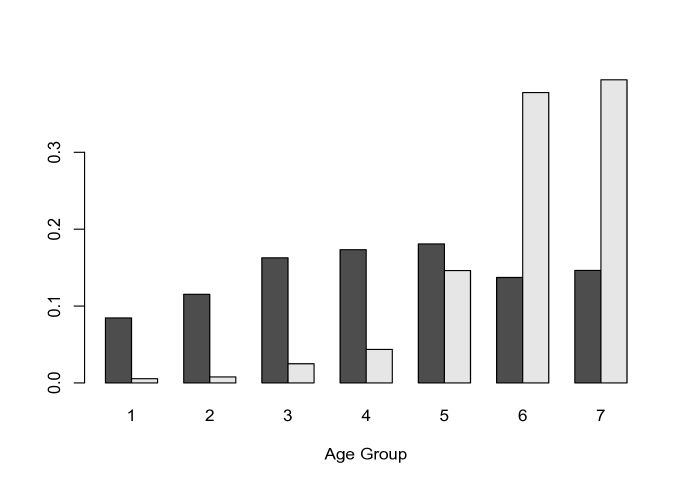
Figure 2: Age distributions from the HarperCollins (dark gray) and CivicScience (light gray) surveys.

Figure 3: Left: Empirical probabilities assigned to category 1 (‘o’ symbol) and category 2 (‘$\times$’ symbol) for each of 6 discovery questions by sampling $B$ as implied by inference for $P(B|A,B^{\prime})$ from the CivicScience data versus marginal distributions of $B$ from the survey data. Right: Empirical probabilities assigned to category 1 (‘o’ symbol), category 2 (‘$\times$’ symbol), and category 3 (‘$\diamond$’ symbol) for each of 6 author interest questions by sampling $B^{\prime}$ as implied by inference for $P(B^{\prime}|A,B)$ from the CivicScience data versus $B^{\prime}$ from the survey data.

After appending the constructed $D^{*}_{s}$ to $(D_{1},D_{2})$, we estimate the DPMPM model on the concatenated data. In the process we impute all missing values in $D_{1}$ and $D_{2}$. As in the simulation studies, we keep $m=50$ of these completed datasets, spacing them far apart in the MCMC iterations to ensure approximate independence. We use the completed versions of $D_{1}$ and $D_{2}$ for multiple imputation inferences.

As a first data fusion inference relevant for marketing strategies, we estimate probabilities of discovery via a given medium for those who have read or are interested in reading a particular author. As evident in Figure 4, high income individuals appear very likely to discover books via recommendations regardless of author. Low income individuals are also likely to discover books through recommendations, but the extent to which this is the case is more variable by author; for instance, low income individuals who have read Christie are more likely to discover new books via recommendations than those who have read Collins. Among individuals who have read Meyer, those with high incomes are very likely to discover books at the library, whereas those with low incomes are not. Low income individuals appear more likely to discover books via the Internet than high income individuals for readers of all authors except Kleypas. In fact, low and high income individuals who have read Kleypas do not appear to differ in terms of discovery.

We also look at author discovery conditional on reading interest and age, as opposed to income. Figure 5 displays inference for $P(B=\mathrm{yes}|B^{\prime}=\mathrm{read},\mathrm{age})$ across age groups for three different combinations of discovery mediums $B$ and authors $B^{\prime}$. There appears to be an increasing trend in discovery via Best Seller List for those who have read Meyer. In other words, older individuals who have read Meyer are more likely to discover new books through the Best Seller List than younger individuals. Quadratic trends are present for discovery via the Internet for those who have read Silverstein and in discovery via Bookstores for those who have read Collins. As evidence of the impact of glue, Figure 5 also displays the multiple imputation point estimates obtained from the DPMPM model fit without using the CivicScience data. In some cases these estimates agree in terms of the trends they suggest (e.g., the middle figure) but sometimes there are fairly stark differences, such as in the leftmost figure.

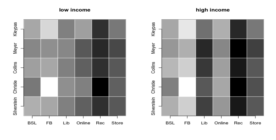
Figure 4: Multiple imputation point estimates for $P(B=\mathrm{yes}|B^{\prime}=\mathrm{read},\mathrm{income})$ for low and high income groups and all mediums $B$ and authors $B^{\prime}$. Black indicates larger probabilities, and white indicates smaller probabilities.

Figure 5: Multiple imputation point estimates and $95\%$ confidence intervals for $P(B=\mathrm{yes}|B^{\prime}=\mathrm{read},\mathrm{age})$ across age groups for three different combinations of mediums $B$ and authors $B^{\prime}$. Open circles refer to the estimates under the DPMPM model applied without any glue. Left: Probability of discovery via Best Seller List given one has read Meyers. Middle: Probability of discovery Online given one has read Silverstein. Right: Probability of discovery via Bookstores given one has read Collins.

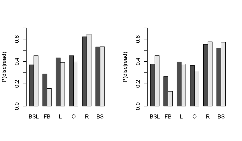
Figure 6: Posterior mean estimates for $P(B=\mathrm{yes}\mid B^{\prime}=\mathrm{read})$ for $B$ representing each of 5 mediums and $B^{\prime}$ representing Silverstein (dark gray) and Christie (light gray) under the model applied with glue (left) and without glue (right).

Finally, we estimate the conditional distributions $P(B\mid B^{\prime})$ for particular discovery mediums and authors. Figure 6 displays these probability distributions for authors Silverstein and Christie, under models applied with and without glue. It appears that fans of Silverstein’s books use Facebook to find out about new books more frequently than fans of Christie’s books; however, both readerships rely on the Best Seller List equally. We note that the glue impacts inference for even these marginal probabilities.

5 Concluding remarks

While useful for marketing purposes in their own right, the results of the HarperCollins and CivicScience data fusion offer some general lessons about integrating online and traditional survey data. First, it is possible to improve inferences by collecting glue, even when the additional data include only portions of the full joint distribution of interest. However, crucially, the glue and survey data should represent the same distribution. Second, data from online polling companies like CivicScience, not surprisingly, are likely to be not representative on some dimensions. However, when one believes that conditional distributions in the polling data are reliable, one can construct appropriate glue from the conditional distributions, as we did in the HarperCollins data fusion. Third, it is important to understand the limitations of the online data. For example, the CivicScience data include very few young people. Thus, the estimate of $P(B\mid A,B^{\prime})$ from the CivicScience data when $A$ refers to a young person has high variance, so that the glue may not offer adequate information about young people.

The simulations with the HarperCollins data also point to interesting directions for future research. In those simulations, adding gender to glue already containing age does not noticeably improve the inferences. In practice, one would expect the cost of collecting glue to increase with the number of variables; hence, in this simulated fusion context, it may not be cost effective to collect gender as part of the glue. This suggests a benefit for research on methods for selecting the variables that most improve the accuracy of data fusion, taking into account the cost of obtaining those variables.

Appendix A Posterior computation

In order to obtain inference under the hierarchical model, we use a Gibbs sampler to simulate from the posterior distribution $p(\{\phi^{(j)}\},Z,V,\alpha,Y^{(mis)}\mid\mathrm{data})$, where $Y^{(mis)}$ refers to all missing values in $Y_{i}=(A_{i},B_{i},B^{\prime}_{i})$ from $D_{1}$ and $D_{2}$, and data refers to all observations of $(A_{i},B_{i},B^{\prime}_{i})$ in $D_{1}$, $D_{2}$, and $D_{s}$. For computational expediency, we need not impute missing values for $D_{s}$, as we are simply using this data to inform nonidentifiable relationships. However, it would be straightforward to impute these missing values just like we impute missing values in $D_{1}$ and $D_{2}$. We now describe the posterior full conditionals for all model parameters.

Full conditional for $Z$

The mixture allocation variables $Z_{i}$, for $i=1,\dots,n$, are updated from categorical distributions with probabilities given by

$$p(Z_{i}=h\mid Y_{i},\pi,\phi)=\frac{\pi_{h}\prod_{j=1}^{p}\phi^{(j)}_{hY_{ij}}}{\sum_{k=1}^{N}\pi_{k}\prod_{j=1}^{p}\phi^{(j)}_{kY_{ij}}}$$ (5)

for $h=1,\dots,N$. For the glue cases, let $J_{i}$ represent the variables in $\{1,\dots,p\}$ that are observed for glue case $i$. The variable $Z_{i}$, $i=1,\dots,n_{s}$, is updated from a categorical distribution with

$$p(Z_{i}=h\mid Y_{i},\pi,\phi)=\frac{\pi_{h}\prod_{j\in J_{i}}\phi^{(j)}_{hY_{ij}}}{\sum_{k=1}^{N}\pi_{k}\prod_{j\in J_{i}}\phi^{(j)}_{kY_{ij}}}$$ (6)

for $h=1,\dots,N$.

Full conditional for $\{\phi^{(j)}\}$

To update $\phi_{h}^{(j)}$, for $h=1,\dots,N$, and $j=1,\dots,p$, sample from a Dirichlet distribution:

$$p(\phi_{h}^{(j)}\mid Y^{(obs)},Z)\propto\mathrm{Dirichlet}\left(\phi_{h}^{(j)};1+\sum_{\{i:Z_{i}=h\}}1(Y_{ij}=1),\dots,1+\sum_{\{i:Z_{i}=h\}}1(Y_{ij}=d_{j})\right),$$ (7)

where the summations are over all survey and glue cases, $i\in\{1,\dots,n+n_{s}\}$.

Full conditional for $V$

The stick-breaking proportions $V_{h}$, for $h=1,\dots,N-1$, can be sampled from Beta distributions:

$$p(V_{h}\mid\alpha,Z)\propto\mathrm{Beta}\left(V_{h};M_{h}+1,\alpha+\sum_{j=h+1}^{N}M_{j}\right),$$ (8)

where $M_{h}=\sum_{i=1}^{n+n_{s}}1(Z_{i}=h)$. Fixing $V_{N}=1$, the probabilities $\pi$ are given by $\pi_{1}=V_{1}$ and $\pi_{h}=V_{h}\prod_{j=1}^{h-1}(1-V_{j})$ for $h=1,\dots,N$.

Full conditional for $\alpha$

The DP precision parameter $\alpha$ can be sampled from a Gamma distribution:

$$p(\alpha\mid V)\propto\mathrm{Gamma}\left(\alpha;N+a_{\alpha}-1,b_{\alpha}-log(\pi_{N})\right).$$ (9)

Imputing $Y^{(mis)}$

Missing $Y_{ij}$ in $D_{1}$ and $D_{2}$ can be imputed by sampling from categorical distributions with the form given in equation (1).

REFERENCES

- D’Orazio et al., (2002) D’Orazio, M., Di Zio, M., and Scanu, M. (2002). Statistical matching and official statistics. Rivista di Statistica Ufficiale, 1:5–24.
- D’Orazio et al., (2006) D’Orazio, M., Di Zio, M., and Scanu, M. (2006). Statistical Matching: Theory and Practice. Wiley, New York.
- Dunson and Xing, (2009) Dunson, D. and Xing, C. (2009). Nonparametric bayes modeling of multivariate categorical data. Journal of the American Statistical Association, 104:1042–1051.
- Gibbs and Su, (2002) Gibbs, A. and Su, F. (2002). On choosing and bounding probability metrics. International Statistical Review, 70:419–435.
- Gilula and McCulloch, (2013) Gilula, Z. and McCulloch, R. (2013). Multilevel categorical data fusion using partially fused data. Journal of Marketing Research, 11:353–377.
- Gilula et al., (2006) Gilula, Z., McCulloch, R., and Rossi, P. (2006). A direct approach to data fusion. Journal of Marketing Research, 43:73–83.
- Goodman, (1974) Goodman, L. (1974). Exploratory latent structure analysis using both identifiable and unidentifiable models. Biometrika, 61:215–231.
- Ishwaran and James, (2001) Ishwaran, H. and James, L. (2001). Gibbs sampling methods for stick-breaking priors. Journal of the American Statistical Association, 96:161–173.
- Ishwaran and Zarepour, (2000) Ishwaran, H. and Zarepour, M. (2000). Markov chain Monte Carlo in approximate Dirichlet and beta two-parameter process hierarchical models. Biometrika, 87:371–390.
- Kadane, (2001) Kadane, J. (2001). Some statistical problems in merging datasets. Journal of Offficial Statistics, 17:423–433.
- Kamakura and Wedel, (1997) Kamakura, W. and Wedel, M. (1997). Statistical data fusion for cross tabulation. Journal of Marketing Research, 34:485–498.
- Kamakura et al., (2003) Kamakura, W., Wedel, M., de Rosa, F., and Mazzon, J. A. (2003). Cross-selling through database marketing: a mixed data factor analyzer for data augmentation and prediction. International Journal of Research in Marketing, 20:45–65.
- Kiesl and Rässler, (2006) Kiesl, H. and Rässler, S. (2006). How valid can data fusion be? IAB Discussion Paper, 15.
- Moriarty and Scheuren, (2001) Moriarty, C. and Scheuren, F. (2001). Statistical matching: A paradigm for assessing the uncertainty in the procedure. Journal of Offficial Statistics, 17:407–422.
- Moriarty and Scheuren, (2003) Moriarty, C. and Scheuren, F. (2003). A note on rubin s statistical matching using file concatenation with adjusted weights and multiple imputations. Journal of Business and Economic Statistics, 21:65–73.
- Pollard, (2002) Pollard (2002). A User’s Guide to Measure Theoretic Probability. Cambridge University Press.
- Rässler, (2002) Rässler, S. (2002). Statistical matching: A frequentist theory, practical applications, and alternative bayesian approaches. In Lecture Notes in Statistics 168, pages 60–63. Springer, New York.
- Rässler, (2004) Rässler, S. (2004). Data fusion: Identification problems, validity, and multiple imputation. Austrian Journal of Statistics, 33.
- Reiter, (2012) Reiter, J. (2012). Bayesian finite population imputation for data fusion. Statistical Sinica, 2:795–811.
- Rodgers, (1994) Rodgers, W. L. (1994). An evaluation of statistical matching. Journal of Business and Economic Statistics, 2:91–102.
- Rubin, (1976) Rubin, D. (1976). Inference and missing data. Biometrika, 63:581–592.
- Rubin, (1986) Rubin, D. (1986). Statistical matching using file concatenation with adjusted weights and multiple imputations. Journal of Business and Economic Statistics, 4:87–94.
- Rubin, (1987) Rubin, D. (1987). Multiple Imputation for Nonresponse in Surveys. John Wiley and Sons, New York.