Construction of Parametric Barrier Functions
for Dynamical Systems using Interval Analysis

Abstract

Recently, barrier certificates have been introduced to prove the safety of continuous or hybrid dynamical systems. A barrier certificate needs to exhibit some barrier function, which partitions the state space in two subsets: the safe subset in which the state can be proved to remain and the complementary subset containing some unsafe region. This approach does not require any reachability analysis, but needs the computation of a valid barrier function, which is difficult when considering general nonlinear systems and barriers. This paper presents a new approach for the construction of barrier functions for nonlinear dynamical systems. The proposed technique searches for the parameters of a parametric barrier function using interval analysis. Complex dynamics can be considered without needing any relaxation of the constraints to be satisfied by the barrier function.

, , ,

1 Introduction

Formal verification aims at proving that a certain behavior or property is fulfilled by a system. Verifying, e.g., the safety property for a system consists in ensuring that it will never reach a dangerous or an unwanted configuration. Safety verification is usually translated into a reachability analysis problem [11, 4, 29, 30, 9]. Starting from an initial region, a system must not reach some unsafe region. Different methods have been considered to address this problem. One may explicitly compute the reachable region and determine whether the system reaches the unsafe region [16]. An alternative idea is to compute an invariant for the system, i.e., a region in which the system is guaranteed to stay [9]. This paper considers a class of invariants determined by barrier functions.

A barrier function [24, 23] partitions the state space and isolates an unsafe region from the part of the state space containing the initial region. In [24] polynomial barriers are considered for polynomial systems and semi-definite programming is used to find satisfying barrier functions. Our aim is to extend the class of considered problems to non-polynomial systems and to non-polynomial barriers. This paper focuses on continuous-time systems.

The design of a barrier function is formulated as a quantified constraints satisfaction problem (QCSP) [6, 25]. Interval analysis is then used to find the parameters of a barrier function such that the QCSP is satisfied. More specifically, the algorithm presented in [18] for robust controller design is adapted and supplemented with some of the pruning schemes found in [7] to solve the QCSP associated to the barrier function design.

The paper is organized as follows. Section 2 introduces some related work. Section 3 defines the notion of barrier functions and formulates the design of barrier functions as a QCSP. Section 4 presents the framework developed to solve the QCSP. Design examples are presented in Section 5. Section 6 concludes the work.

In what follows small italic letters $x$ represent real variables while real vectors $\mathbf{x}$ are in bold. Intervals $\left[x\right]$ and interval vectors (boxes) $\mathbf{\left[x\right]}$ are represented between brackets. We denote by $\mathbb{IR}$ the set of closed intervals over $\mathbb{R}$, the set of real numbers. Data structures or sets $\mathcal{S}$ are in upper-case calligraphic. The derivative of a function $x$ with respect to time $t$ is denoted by $\dot{x}$.

2 Related work

To prove the safety of a dynamical system, different approaches have been proposed [15, 31, 19, 4, 11, 30, 9]. One way is to explicitly compute an outer approximation of the reachable region from the initial region, i.e., the set of possible values for the initial state. If it does not intersect the unsafe region, then the system is safe. In [4, 30, 14] the reachable region is computed for linear hybrid systems for a finite time horizon using geometric representation such as polyhedra. The reachable region for non-linear systems is computed in [28] using an abstraction of the non-linear systems by a linear system expressed in a new system of coordinates. The reachability of a non-linear system is formulated as an optimization problem in [10]. In [8], the Picard-Lindelöf operator is combined with Taylor models to find the reachable region for non-linear hybrid systems. The main downside of the reachability approach is the introduction of over-approximations during the computations which may lead to difficulties to decide whether the system is safe.

An alternative way to address the safety problem is by exhibiting an invariant region in which the system remains. If the invariant does not intersect the unsafe region then the safety of the system is proved. One way to find such an invariant is by using stability properties of the considered dynamical system [13] and to search for a Lyapunov function. In [22] a sum of squares decomposition and a semi-definite programming approach are employed to find a Lyapunov function for a system with polynomial dynamics. A template approach is considered in [27] to find Lyapunov functions using a branch and relax scheme and linear programming to solve the induced constraints. A more general idea about invariants is introduced in [24]. Instead of looking for a function that fulfills some stability conditions, a function is searched that separates the initial region from the unsafe region. This idea is extended in [16] to search for invariants in conjunctive normal form for hybrid systems.

3 Formulation

This section recalls the safety characterization introduced in [24] for continuous-time systems using barrier functions.

3.1 Safety for continuous-time systems

Consider the autonomous continuous-time perturbed dynamical system

$$\mathbf{\dot{x}}=f(\mathbf{x},\mathbf{d}),$$ (1)

where $\mathbf{x}\in\mathcal{X}\subseteq\mathbb{R}^{n}$ is the state vector and $\mathbf{d}\in\mathcal{D}$ is a constant and bounded disturbance. The set of possible initial states at $t=0$ is denoted $\mathcal{X}_{0}\subset\mathcal{X}$. There is some unsafe subset $\mathcal{X}_{u}\subseteq\mathcal{X}$ that shall not be reached by the system, whatever $\mathbf{x}_{0}\mathcal{\in X}_{0}$ at time $t=0$ and whatever $\mathbf{d}\in\mathcal{D}$. We assume that classical hypotheses (see, e.g., [5]) on $f$ are satisfied so that (1) has a unique solution $\mathbf{x}(t,\mathbf{x}_{0},\mathbf{d})\in\mathcal{X}$ for any given initial value $\mathbf{x}_{0}\mathcal{\in X}_{0}$ at time $t=0$ and any $\mathbf{d}\in\mathcal{D}$.

Definition 1.

The dynamical system (1) is safe if $\forall\mathbf{x}_{0}\in\mathcal{X}_{0}$, $\forall\mathbf{d}\in\mathcal{D}$ and $\forall t\geqslant 0$, $\mathbf{x}(t,\mathbf{x}_{0},\mathbf{d})\notin\mathcal{X}_{u}$.

3.2 Barrier certificates

A way to prove that (1) is safe is by the barrier certificate approach introduced in [24]. A barrier is a differentiable function $B:\mathcal{X}\to\mathbb{R}$ that partitions the state space $\mathcal{X}$ into $\mathcal{X}_{-}$ where $B(\mathbf{x})\leqslant 0$ and $\mathcal{X}_{+}$ where $B(\mathbf{x})>0$ such that $\mathcal{X}_{0}\subseteq\mathcal{X}_{-}$ and $\mathcal{X}_{u}\subseteq\mathcal{X}_{+}$. Moreover, $B$ has to be such that $\forall\mathbf{x}_{0}\in\mathcal{X}_{0}$, $\forall\mathbf{d}\in\mathcal{D}$, $\forall t\geqslant 0$, $B(\mathbf{x}(t,\mathbf{x}_{0},\mathbf{d}))\leqslant 0$.

Proving that $B(\mathbf{x}(t,\mathbf{x}_{0},\mathbf{d}))\leqslant 0$ requires an evaluation of the solution of (1) for all $\mathbf{x}_{0}\in\mathcal{X}_{0}$ and $\mathbf{d}\in\mathcal{D}$. Alternatively, [24] provides some sufficient conditions a barrier function has to satisfy to prove the safety of a dynamical system, see Theorem 1.

Theorem 1.

Consider the dynamical system (1) and the sets $\mathcal{X}$, $\mathcal{D}$, $\mathcal{X}_{0}$ and $\mathcal{X}_{u}$. If there exists a function $B:\mathcal{X}\to\mathbb{R}$ such that

$$\forall\mathbf{x\in}\mathcal{X}_{0},\quad B(\mathbf{x})\leqslant 0,$$ (2)

$$\forall\mathbf{x\in}\mathcal{X}_{u},\quad B(\mathbf{x})>0,$$ (3)

$\forall\mathbf{x}\in\mathcal{X},\,\forall\mathbf{d\in\mathcal{D}}$,

$$B(\mathbf{x})=0\implies\left\langle\frac{\partial B(\mathbf{x})}{\partial\mathbf{x}},f(\mathbf{x},\mathbf{d})\right\rangle<0,$$ (4)

then (1) is safe.

In (4) $\left\langle.,.\right\rangle$ stands for the dot product in $\mathbb{R}^{n}$. In Theorem 1, (2) and (3) ensure that $\mathcal{X}_{0}\subseteq\mathcal{X}_{-}$, and $\mathcal{X}_{u}\subseteq\mathcal{X}_{+}$, while (4) states that if $\mathbf{x}$ is on the border between $\mathcal{X}_{-}$ and $\mathcal{X}_{+}$ (i.e., $B(\mathbf{x})=0$), then the dynamics $f$ pushes the state back in $\mathcal{X}_{-}$ whatever the value of the disturbance $\mathbf{d}$.

3.3 Parametric barrier functions

The search for a barrier $B$ is challenging since it is over a functional space. As in [24], this paper considers barriers belonging to a family of parametric functions (or templates) $B(\mathbf{x},\mathbf{p})$ depending on a parameter vector $\mathbf{p}\in\mathcal{P}\subseteq\mathbb{R}^{m}$. Then one may search for some parameter value $\mathbf{p}$ such that $B(\mathbf{x},\mathbf{p})$ satisfies (2)-(4).

If there is no $\mathbf{p}\in\mathcal{P}$ such that $B(\mathbf{x},\mathbf{p})$ satisfies (2)-(4), this does not mean that the system is not safe: other structures of functions $B(\mathbf{x},\mathbf{p})$ could provide a barrier certificate.

4 Characterization using interval analysis

This section presents an approach to find a barrier function that fulfills the constraints of Theorem 1. These constraints are first reformulated to cast the design of a barrier function as a quantified constraint satisfaction problem (QCSP)[25].

4.1 Constraint satisfaction problem

Assume that there exist some functions $g_{0}:\mathcal{X}\to\mathbb{R}$ and $g_{u}:\mathcal{X}\to\mathbb{R}$, such that

$$\mathcal{X}_{0}=\{\mathbf{x}\in\mathcal{X}\,|\,g_{0}(\mathbf{x})\leqslant 0\}$$ (5)

and

$$\mathcal{X}_{u}=\{\mathbf{x}\in\mathcal{X}\,|\,g_{u}(\mathbf{x})\leqslant 0\}.$$ (6)

Theorem 1 may be reformulated as follows.

Proposition 2.

If $\exists\mathbf{p}\in\mathcal{P}$ such that $\forall\mathbf{x}\in\mathcal{X}$, $\forall\mathbf{d}\in\mathcal{D}$

$$\xi\left(\mathbf{x},\mathbf{p},\mathbf{d}\right)= \left(g_{0}(\mathbf{x})>0\lor B(\mathbf{x},\mathbf{p})\leqslant 0\right)$$ (7)

$$\land\left(g_{u}(\mathbf{x})>0\lor B(\mathbf{x},\mathbf{p})>0\right)$$ (8)

$$\land\left(B(\mathbf{x},\mathbf{p})\neq 0\lor\left\langle\frac{\partial B}{\partial\mathbf{x}}(\mathbf{x},\mathbf{p}),f(\mathbf{x},\mathbf{d})\right\rangle<0\right)$$ (9)

holds true, then the dynamical system (1) is safe.

The first component of $\xi\left(\mathbf{x},\mathbf{p},\mathbf{d}\right)$,

$$\xi_{\text{0}}\left(\mathbf{x},\mathbf{p}\right)=\left(g_{0}(\mathbf{x})>0\lor B(\mathbf{x},\mathbf{p})\leqslant 0\right)$$ (10)

may be rewritten as

$$\xi_{\text{0}}\left(\mathbf{x},\mathbf{p}\right)=\left(g_{0}(\mathbf{x})\leqslant 0\implies B(\mathbf{x},\mathbf{p})\leqslant 0\right),$$

see, e.g., [12]. If $\xi_{\text{0}}\left(\mathbf{x},\mathbf{p}\right)$ holds true for some $\mathbf{p}\in\mathcal{P}$ and $\mathbf{x}\in\mathcal{X}$, then one has either $\mathbf{x}\in\mathcal{X}_{0}$ and $B(\mathbf{x},\mathbf{p})\leqslant 0$, or $\mathbf{x}\notin\mathcal{X}_{0}$. In both cases, (2) is satisfied. A similar derivation can be made for the second component of $\xi\left(\mathbf{x},\mathbf{p},\mathbf{d}\right)$ to encode (3),

$$\xi_{u}(\mathbf{x},\mathbf{p})=\left(g_{u}(\mathbf{x})>0\lor B(\mathbf{x},\mathbf{p})>0\right).$$ (11)

Now, one may rewrite the last component of $t\left(\mathbf{x},\mathbf{p},\mathbf{d}\right)$,

$$\xi_{b}(\mathbf{x},\mathbf{p},\mathbf{d)}=\left(B(\mathbf{x},\mathbf{p})\neq 0\lor\left\langle\frac{\partial B}{\partial x}(\mathbf{x},\mathbf{p}),f(\mathbf{x},\mathbf{d})\right\rangle<0\right)$$ (12)

as

$$\xi_{b}(\mathbf{x},\mathbf{p},\mathbf{d)}=\\ \left(B(\mathbf{x},\mathbf{p})=0\implies\left\langle\frac{\partial B}{\partial\mathbf{x}}(\mathbf{x},\mathbf{p}),f(\mathbf{x},\mathbf{d})\right\rangle<0\right),$$ (13)

which corresponds to (4). If $\exists\mathbf{p}\in\mathcal{P}$ such that $\forall\mathbf{x}\in\mathcal{X}$, $\forall\mathbf{d}\in\mathcal{D}$, $\xi\left(\mathbf{x},\mathbf{p},\mathbf{d}\right)$ holds true, then the conditions of Theorem 1 are satisfied and (1) is safe. ∎

In [24], (9) is relaxed into

$$\xi_{\text{b}}\left(\mathbf{x},\mathbf{p},\mathbf{d}\right)=\left(\left\langle\frac{\partial B}{\partial\mathbf{x}}(\mathbf{x},\mathbf{p}),f(\mathbf{x},\mathbf{d})\right\rangle<0\right),$$ (14)

with the consequence of possible elimination of barrier functions that would satisfy (9) for some $\mathbf{p}$ but not (14). Our aim in this paper is to design barrier functions without resorting to this relaxation by considering methods from interval analysis [17] which allow to consider strongly nonlinear dynamics and barrier functions.

4.2 Solving the constraints

To find a valid barrier function one needs to find some $\mathbf{p}\in\mathcal{P}$ such that $B(\mathbf{x},\mathbf{p})$ satisfies the conditions of Proposition 2. For that purpose, the Computable Sufficient Conditions-Feasible Point Searcher (CSC-FPS) algorithm [18] is adapted.

In what follows, we assume that $\mathcal{X}$, $\mathcal{D}$, and $\mathcal{P}$ are boxes, i.e., $\mathcal{X}=\left[\mathbf{x}\right]$, $\mathcal{D}=\left[\mathbf{d}\right]$, and $\mathcal{P}=\left[\mathbf{p}\right]$. CSC-FPS may also be applied when $\mathcal{X}$, $\mathcal{D}$, and $\mathcal{P}$ consist of a union of non-overlapping boxes.

Consider some function $g:\mathbb{R}^{n}\times\mathbb{R}^{m}\rightarrow\mathbb{R}^{k}$ and some box $\left[\mathbf{z}\right]\in\mathbb{IR}^{k}$. CSC-FPS is designed to determine whether

$$\exists\mathbf{p}\in\left[\mathbf{p}\right],\mbox{ }\forall\mathbf{x}\in\left[\mathbf{x}\right],\mbox{ }g\left(\mathbf{x},\mathbf{p}\right)\in\left[\mathbf{z}\right]$$ (15)

and to provide some satisfying $\mathbf{p}$. We extend CSC-FPS to handle conjunctions and disjunctions of constraints and supplement it with efficient pruning techniques involving contractors provided by interval analysis [17].

FPS branches over the parameter search box $\left[\mathbf{p}\right]$. Branching is performed based on the results provided by CSC. For a given box $\mathbf{\left[p\right]}_{0}\subseteq\left[\mathbf{p}\right]$, CSC returns true when it manages to prove that (15) is satisfied for some $\mathbf{p}\in\mathbf{\left[p\right]}_{0}$. CSC returns false when it is able to show that there is no $\mathbf{p}\in\mathbf{\left[p\right]}_{0}$ satisfying (15). CSC returns unknown in the other cases.

In Proposition 2, $\xi\left(\mathbf{x},\mathbf{p},\mathbf{d}\right)$ consists of the conjunction of three terms of the form

$$\tau\left(\mathbf{x},\mathbf{p},\mathbf{d}\right)=\left(u(\mathbf{x},\mathbf{p})\in\mathcal{A}\right)\lor\left(v(\mathbf{x},\mathbf{p,d})\in\mathcal{B}\right).$$ (16)

For $\xi_{0}(\mathbf{x},\mathbf{p})$, defined in (7),

$$\mathcal{A}=\left]0,+\infty\right]\mbox{ and }\mathcal{B}=\left]-\infty,0\right];$$ (17)

for $\xi_{u}(\mathbf{x},\mathbf{p})$, defined in (8),

$$\mathcal{A}=\left]0,+\infty\right]\mbox{ and }\mathcal{B}=\left]0,+\infty\right[;$$ (18)

for $\xi_{b}(\mathbf{x},\mathbf{p},\mathbf{d})$, defined in (9),

$$\mathcal{A}=\left]-\infty,0\right[\cup\left]0,+\infty\right[\mbox{ and }\mathcal{B}=\left]-\infty,0\right[.$$ (19)

To illustrate the main ideas of CSC-FPS combined with contractors, one focuses on the generic QCSP

$$\exists\mathbf{p}\in\left[\mathbf{p}\right],\forall\mathbf{x}\in\mathbf{\left[x\right],\forall d\in}\left[\mathbf{d}\right],\,\tau\left(\mathbf{x},\mathbf{p},\mathbf{d}\right)\mbox{ holds true}.$$ (20)

Finding a solution for such QCSP involves three steps: validation, reduction of the parameter and state spaces, and bisection.

4.2.1 Validation

In the validation step, one tries to prove that some vector $\mathbf{p}\in\mathbf{\left[p\right]}$ is such that $\forall\mathbf{x}\in\mathbf{\left[x\right]}$, $\forall\mathbf{d\in}\left[\mathbf{d}\right]$, $\tau\left(\mathbf{x},\mathbf{p,d}\right)$ holds true. By definition of $\tau\left(\mathbf{x},\mathbf{p},\mathbf{d}\right)$, one has to prove that

$$\exists\mathbf{p}\in\left[\mathbf{p}\right],\forall\mathbf{x}\in\left[\mathbf{x}\right],\forall\mathbf{d}\in\left[\mathbf{d}\right],\\ \left(u(\mathbf{x},\mathbf{p})\in\mathcal{A}\right)\lor\left(v(\mathbf{x},\mathbf{p},\mathbf{d})\in\mathcal{B}\right).$$ (21)

For that purpose, one chooses some arbitrary $\mathbf{p}\in\mathbf{\left[p\right]}$ and evaluates the set of values $u\left(\left[\mathbf{x}\right],\mathbf{p}\right)=\left\{u\left(\mathbf{x},\mathbf{p}\right)\mid\mathbf{x}\in\mathbf{\left[\mathbf{x}\right]}\right\}$ and $v\left(\left[\mathbf{x}\right],\mathbf{p,\left[d\right]}\right)=\{v\left(\mathbf{x},\mathbf{p},\mathbf{d}\right)\mid\mathbf{x}\in\mathbf{\left[\mathbf{x}\right]},\mathbf{d}\in\mathbf{\left[d\right]}\}$ taken by $u(\mathbf{x},\mathbf{p})$ and $v(\mathbf{x},\mathbf{p,d})$ for all $\mathbf{x}\in\mathbf{\left[\mathbf{x}\right]}$ and for all $\mathbf{d}\in\left[\mathbf{d}\right]$. Outer-approximations of $u\left(\left[\mathbf{x}\right],\mathbf{p}\right)$ and $v\left(\left[\mathbf{x}\right],\mathbf{p,\left[d\right]}\right)$ are easily obtained using inclusion functions provided by interval analysis.

Definition 3.

An inclusion function $[f]:\mathbb{IR}^{n}\to\mathbb{IR}^{k}$ for a function $f:\mathbb{R}^{n}\to\mathbb{R}^{k}$ satisfies for all $\left[\mathbf{x}\right]\in\mathbb{IR}^{n}$,

$$f\left(\left[\mathbf{x}\right]\right)=\left\{f(\mathbf{x})\mid\mathbf{x}\in\left[\mathbf{x}\right]\right\}\subseteq\left[f\right]\left(\left[\mathbf{x}\right]\right).$$ (22)

The natural inclusion function is the simplest to obtain: all occurrences of the real variables are replaced by their interval counterpart and all arithmetic operations are evaluated using interval arithmetic. More sophisticated inclusion functions such as the centered form, or the Taylor inclusion function may also be used, see [17].

Using inclusion functions, one may evaluate whether

$$[u](\mathbf{\left[x\right]},\mathbf{p})\subseteq\mathcal{A}\text{\quad or\quad}[v](\mathbf{\left[x\right]},\mathbf{p,\left[d\right]})\subseteq\mathcal{B}\quad\text{holds true}$$

for the various $\mathcal{A}$ and $\mathcal{B}$ defined in (17), (18), and (19).

Different choices can be considered for $\mathbf{p}$: one can take a random point in $\mathbf{\left[p\right]}$, the middle, or one of the edges of $\mathbf{\left[p\right]}$. Here, only the middle of $\mathbf{\left[p\right]}$ is considered.

4.2.2 Reduction of the parameter and state spaces

To facilitate the search for $\mathbf{p}\in\mathbf{\left[p\right]}$ one may previously eliminate parts of $\mathbf{\left[p\right]}$ which may be proved not to contain any $\mathbf{p}$ satisfying (21). The elimination process can be done by evaluation or by using contractors [7].

Evaluation

From (21) one deduces that a box $\mathbf{\left[p\right]}$ can be eliminated, i.e., shown not to contain any $\mathbf{p}$ satisfying (16), if

$$\forall\mathbf{p}\in\mathbf{\left[p\right]},\exists\mathbf{x}\in\left[\mathbf{x}\right],\exists\mathbf{d}\in\left[\mathbf{d}\right],\\ u(\mathbf{x},\mathbf{p})\subseteq\overline{\mathcal{A}}\wedge v(\mathbf{x},\mathbf{p,d})\subseteq\overline{\mathcal{B}},$$ (23)

where $\mathcal{\overline{A}}=\mathbb{R}\setminus\mathcal{A}$ and $\mathcal{\overline{B}}=\mathbb{R}\setminus\mathcal{B}$. Using again an inclusion function, one may verify whether $[u](\mathbf{x},\mathbf{\left[p\right]})\subseteq\overline{\mathcal{A}}$ and $[v](\mathbf{x},\mathbf{\left[p\right],d})\subseteq\overline{\mathcal{B}}$ for some $\mathbf{x}\in\mathbf{\left[x\right]}$ and $\mathbf{d\in\left[d\right]}$ and thus eliminate the box $\mathbf{\left[p\right]}$.

One may easily verify (7) and (8) since $\overline{\mathcal{A}}$ and $\overline{\mathcal{B}}$ are unbounded and may contain $[u](\mathbf{x},\mathbf{\left[p\right]})$ and $[v](\mathbf{x},\mathbf{\left[p\right],d})$. For (9) the inclusion is impossible to prove except in degenerate cases since $\overline{\mathcal{A}}=\left\{0\right\}$.

Contractors

Consider some function $g:\mathbb{R}^{n}\rightarrow\mathbb{R}^{k}$ and some set $\mathcal{Z}\subset\mathbb{R}^{k}$.

Definition 4.

A contractor $\mathcal{C}_{c}:\mathbb{IR}^{n}\to\mathbb{IR}^{n}$ associated to the generic constraint

$$c:g(\mathbf{x})\in\mathcal{Z}$$ (24)

is a function taking a box $\left[\mathbf{x}\right]$ as input and returning a box $\mathcal{C}_{c}\left(\left[\mathbf{x}\right]\right)$ satisfying

$$\mathcal{C}_{c}\left(\left[\mathbf{x}\right]\right)\subseteq\left[\mathbf{x}\right]$$ (25)

and

$$g\left(\left[\mathbf{x}\right]\right)\cap\mathcal{Z}=g\left(\mathcal{C}_{c}\left(\left[\mathbf{x}\right]\right)\right)\cap\mathcal{Z}.$$ (26)

$\mathcal{C}_{c}$ provides a box containing the solutions of $g(\mathbf{x})\in\mathcal{Z}$ included in $\left[\mathbf{x}\right]$: (25) ensures that the returned box is included in $\mathbf{\left[x\right]}$ and (26) ensures that no solution of $g(\mathbf{x})\in\mathcal{Z}$ in $\mathbf{\left[x\right]}$ is lost.

Consider now two functions $g_{1}:\mathbb{R}^{n}\rightarrow\mathbb{R}^{k_{1}}$ and $g_{2}:\mathbb{R}^{n}\rightarrow\mathbb{R}^{k_{2}}$, two sets $\mathcal{Z}_{1}\subset\mathbb{R}^{k_{1}}$ and $\mathcal{Z}_{2}\subset\mathbb{R}^{k_{2}}$, and the associated constraints $c_{1}:g_{1}(\mathbf{\left[x\right]})\subseteq\mathcal{Z}_{1}$ and $c_{2}:g_{2}(\mathbf{\left[x\right]})\subseteq\mathcal{Z}_{2}$. Assume that two contractors $\mathcal{C}_{c_{1}}$ and $\mathcal{C}_{c_{2}}$ are available for $c_{1}$ and $c_{2}$. A contractor $\mathcal{C}_{c_{1}\land c_{2}}$ for the conjunction $c_{1}\wedge c_{2}$ of $c_{1}$ and $c_{2}$ may be obtained as

$$\mathcal{C}_{c_{1}\land c_{2}}(\mathbf{\left[x\right]})=\mathcal{C}_{c_{1}}(\mathbf{\left[x\right]})\cap\mathcal{C}_{c_{2}}(\mathbf{\left[x\right]}),$$ (27)

or by composition of contractors

$$\mathcal{C}_{c_{1}\land c_{2}}(\mathbf{\left[x\right]})=\mathcal{C}_{c_{2}}(\mathcal{C}_{c_{1}}(\mathbf{\left[x\right]})).$$ (28)

A contractor $\mathcal{C}_{c_{1}\vee c_{2}}$ for the disjunction $c_{1}\vee c_{2}$ of $c_{1}$ and $c_{2}$ may be obtained as follows

$$\mathcal{C}_{c_{1}\lor c_{2}}(\mathbf{\left[x\right]})=\Box\{\mathcal{C}_{c_{1}}(\mathbf{\left[x\right]})\cup\mathcal{C}_{c_{2}}(\mathbf{\left[x\right]})\},$$ (29)

see [7], with $\Box\{\cdot\}$ the interval hull of a set.

Using a contractor $\mathcal{C}_{c}$ for (24), one is able to characterize some $\left[\tilde{\mathbf{x}}\right]\subset\left[\mathbf{x}\right]$ such that $\forall\mathbf{x}\in\left[\tilde{\mathbf{x}}\right]$, $g(\mathbf{x})\notin\mathcal{Z}$.

Proposition 5.

Consider a box $\mathbf{\left[x\right]}$, the elementary constraint (24), and the contracted box $\mathcal{C}_{c}\left(\mathbf{\left[x\right]}\right)\subseteq\left[\mathbf{x}\right]$. Then,

$$\forall\mathbf{x}\in\left[\mathbf{x}\right]\backslash\mathcal{C}_{c}\left(\mathbf{\left[x\right]}\right),\mbox{ one has }g(\mathbf{x})\notin\mathcal{Z},$$ (30)

where $\left[\mathbf{x}\right]\backslash\mathcal{C}_{c}\left(\mathbf{\left[x\right]}\right)$ denotes the box $\left[\mathbf{x}\right]$ deprived from $\mathcal{C}_{c}\left(\mathbf{\left[x\right]}\right)$, which is not necessarily a box.

Consider $\mathbf{x}\in\left[\mathbf{x}\right]\backslash\mathcal{C}_{c}\left(\mathbf{\left[x\right]}\right)$ and assume that $g(\mathbf{x})\in\mathcal{Z}$. Since $g(\mathbf{x})\in\mathcal{Z}$ and $\mathbf{x}\in\left[\mathbf{x}\right]$, one should have $\mathbf{x}\in\mathcal{C}_{c}\left(\mathbf{\left[x\right]}\right)$, according to (26), which contradicts the fact that $\mathbf{x}\in\left[\mathbf{x}\right]\backslash\mathcal{C}_{c}\left(\mathbf{\left[x\right]}\right)$. ∎

Proposition 5 can be used to eliminate $\mathbf{\left[p\right]}$ or a part of $\mathbf{\left[p\right]}$ for which it is not possible to find any $\mathbf{p}$ satisfying (21). Consider the constraint

$$\tau:\left(u(\mathbf{x},\mathbf{p})\in\mathcal{A}\right)\lor\left(v(\mathbf{x},\mathbf{p},\mathbf{d})\in\mathcal{B}\right)$$ (31)

and a contractor $\mathcal{C}_{\tau}$ for this constraint. It involves elementary contractors for the components of the disjunction in (31), combined as in (29). For the boxes $\left[\mathbf{x}\right]$, $\left[\mathbf{p}\right]$, and $\mathbf{\left[d\right]}$, one gets

$$\begin{pmatrix}\left[\mathbf{x}\right]^{\prime},&\left[\mathbf{p}\right]^{\prime},&\mathbf{\left[d\right]}^{\prime}\end{pmatrix}=\mathcal{C}_{\tau}\begin{pmatrix}\left[\mathbf{x}\right],&\left[\mathbf{p}\right],&\mathbf{\left[d\right]}\end{pmatrix},$$ (32)

where $\left[\mathbf{x}\right]^{\prime}$, $\left[\mathbf{p}\right]^{\prime}$, and $\left[\mathbf{d}\right]^{\prime}$ are the contracted boxes. Three cases may then be considered.

1. If $\mathbf{\left[p\right]}\setminus\mathbf{\left[p\right]}^{\prime}\neq\emptyset$, then $\forall\mathbf{p}\in\mathbf{\left[p\right]\setminus}\mathbf{\left[p\right]}^{\prime},\,\forall\mathbf{x}\in\mathbf{\left[x\right]},\,\forall\mathbf{d}\in\mathbf{\left[d\right]}$,

   $$u(\mathbf{x},\mathbf{p})\notin\mathcal{A}\land v(\mathbf{x},\mathbf{p},\mathbf{d})\notin\mathcal{B},$$ (33)

   and there is no $\mathbf{p}\in\left[\mathbf{p}\right]\setminus\mathbf{\left[p\right]}^{\prime}$ such that (31) holds true for all $\mathbf{x}\in\mathbf{\left[x\right]}$ and for all $\mathbf{d}\in\mathbf{\left[d\right]}$. Consequently, the search space for $\mathbf{p}$ can be reduced to $\mathbf{\left[p\right]}^{\prime}$, see Figure 1 (a).

2. If $\mathbf{\left[x\right]}\setminus\mathbf{\left[x\right]}^{\prime}\neq\emptyset$ then, from Proposition 5, one has $\forall\mathbf{p\in}\mathbf{\left[p\right]},\mathbf{\,\forall x\in}\mathbf{\left[x\right]\setminus}\mathbf{\left[x\right]}^{\prime},\mathbf{\,\forall d\in}\mathbf{\left[d\right]}$,

   $$u(\mathbf{x},\mathbf{p})\notin\mathcal{A}\land v(\mathbf{x},\mathbf{p},\mathbf{d})\notin\mathcal{B},$$ (34)

   and there is no $\mathbf{p}\in\left[\mathbf{p}\right]$ such that (31) holds true for all $\textbf{x}\in\left[\mathbf{x}\right]$, see Figure 1 (b).

3. If $\mathbf{\left[d\right]}\setminus\mathbf{\left[d\right]}^{\prime}\neq\emptyset$, then $\forall\mathbf{p}\in\mathbf{\left[p\right]},\,\forall\mathbf{x}\in\mathbf{\left[x\right]},\,\forall\mathbf{d}\in\mathbf{\left[d\right]}\setminus\mathbf{\left[d\right]}^{\prime}$,

   $$u(\mathbf{x},\mathbf{p})\notin\mathcal{A}\land v(\mathbf{x},\mathbf{p},\mathbf{d})\notin\mathcal{B},$$ (35)

   and there is no $\mathbf{p}\in\left[\mathbf{p}\right]$ such that (31) holds true for all $\textbf{d}\in\left[\mathbf{d}\right]$, see Figure 1 (b).

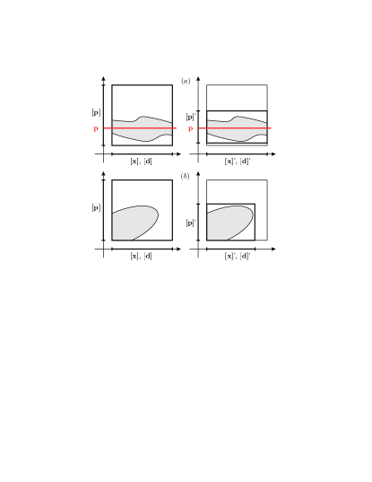
Figure 1: Contractions using $\mathcal{C}_{\tau}$; the set for which (31) is satisfied is in gray; (a) $\mathbf{\left[p\right]}\setminus\mathbf{\left[p\right]}^{\prime}\neq\emptyset$ and the search space for satisfying $\mathbf{p}$ can be reduced to $\left[\mathbf{p}\right]^{\prime};$ (b) $\mathbf{\left[x\right]}^{\prime}\neq\mathbf{\left[x\right]}$ or $\mathbf{\left[d\right]}^{\prime}\neq\mathbf{\left[d\right]}$, it is thus not possible to find some $\mathbf{p}\in\left[\mathbf{p}\right]$ such that (31) is satisfied for all $\mathbf{x}\in\left[\mathbf{x}\right]$ and all $\mathbf{d}\in\left[\mathbf{d}\right]$.

One can reduce the size of the sets for the state $\mathbf{x}$ and the disturbance $\mathbf{d}$ on which (31) has to be verified using the contraction on the negation of this constraint. Consider the negation $\overline{\tau}$ of $\tau$

$$\overline{\tau}=\left(u(\mathbf{x},\mathbf{p})\in\mathcal{\overline{A}}\right)\land\left(v(\mathbf{x},\mathbf{p},\mathbf{d})\in\mathcal{\overline{B}}\right)$$ (36)

and a contractor $\mathcal{C}_{\overline{\tau}}$ for this constraint. Assume that after applying $\mathcal{C}_{\overline{\tau}}$ for the boxes $\left[\mathbf{x}\right]$, $\mathbf{\left[p\right]}$, and $\mathbf{\left[d\right]}$, one gets

$$\begin{pmatrix}\left[\mathbf{x}\right]",&\left[\mathbf{p}\right]",&\mathbf{\left[d\right]}"\end{pmatrix}=\mathcal{C}_{\overline{\tau}}\begin{pmatrix}\left[\mathbf{x}\right],&\left[\mathbf{p}\right],&\mathbf{\left[d\right]}\end{pmatrix}.$$ (37)

From Proposition 5, one knows that

$$\forall\left(\mathbf{x},\mathbf{p},\mathbf{d}\right)\in\left(\mathbf{\left[x\right]}\times\mathbf{\left[p\right]}\times\left[\mathbf{d}\right]\right)\setminus\left(\left[\mathbf{x}\right]"\times\left[\mathbf{p}\right]"\times\left[\mathbf{d}\right]"\right),\\ u(\mathbf{x},\mathbf{p})\in\mathcal{A}\lor v(\mathbf{x},\mathbf{p},\mathbf{d})\in\mathcal{B}.$$ (38)

Indeed, if $\left[\mathbf{p}\right]"=\left[\mathbf{p}\right]$, one can focus on the search for some $\mathbf{p}\in\mathbf{\left[p\right]}$ satisfying (31) by considering only $\mathbf{\left[x\right]}"\times\left[\mathbf{d}\right]"$, since for all $\left(\mathbf{x},\mathbf{d}\right)\in\left(\mathbf{\left[x\right]}\times\left[\mathbf{d}\right]\right)\setminus\left(\left[\mathbf{x}\right]"\times\left[\mathbf{d}\right]"\right)$, (31) is satisfied for all $\mathbf{p}\in\mathbf{\left[p\right]}$, see Figure 2 (a).

Now, if $\left[\mathbf{p}\right]"\neq\left[\mathbf{p}\right]$, then any $\mathbf{p}\in\left[\mathbf{p}\right]\setminus\left[\mathbf{p}\right]"$ will satisfy (31) for all $\left(\mathbf{x},\mathbf{d}\right)\in\left(\mathbf{\left[x\right]}\times\left[\mathbf{d}\right]\right)$, see Figure 2 (b).

Figure 2: Contractions using $\mathcal{C}_{\overline{\tau}}$; the set for which (36) is satisfied is in white; (a) $\mathbf{\left[x\right]}"\neq\mathbf{\left[x\right]}$ and/or $\mathbf{\left[d\right]}"\neq\mathbf{\left[d\right]}$ and one has only to find some suitable $\mathbf{p\in\left[\mathbf{p}\right]}$ such that (31) is satisfied for all $\mathbf{x}\in\left[\mathbf{x}\right]"$ and all $\mathbf{d}\in\left[\mathbf{d}\right]"$; (b) $\mathbf{\left[p\right]}"\neq\mathbf{\left[p\right]}$, one may choose any $\mathbf{p}\in\left[\mathbf{p}\right]\setminus\left[\mathbf{p}\right]"$ (for example the value of $\mathbf{p}$ indicated in red) and (31) will hold true for all $\left(\mathbf{x},\mathbf{d}\right)\in\left(\mathbf{\left[x\right]}\times\left[\mathbf{d}\right]\right)$.

4.2.3 Bisection

One is unable to decide whether some $\mathbf{p}\in\left[\mathbf{p}\right]$ satisfies (21) when

$$[u](\mathbf{\left[x\right]},\mathbf{p})\cap\mathcal{A}\neq\emptyset\text{ and $\left[u\right]$$\left(\mathbf{\left[x\right]},\mathbf{p}\right)\nsubseteq\mathcal{A}$}$$ (39)

or when

$$[v](\mathbf{\left[x\right]},\mathbf{p,\left[d\right]})\cap\mathcal{B}\neq\emptyset\,\text{and}\,[v](\mathbf{\left[x\right]},\mathbf{p,\left[d\right]})\nsubseteq\mathcal{B}.$$ (40)

This situation occurs in two cases. First, when the selected $\mathbf{p}$ does not satisfy (21) for all $\mathbf{x}\in\left[\mathbf{x}\right]$ and for all $\mathbf{d}\in\left[\mathbf{d}\right]$. Second, when inclusion functions introduce some pessimism, i.e., they provide an over-approximation of the range of functions over intervals.

To address both cases, one may perform bisections of $\left[\mathbf{x}\right]\times\left[\mathbf{d}\right]$ and try to verify (21) on the resulting sub-boxes for the same $\mathbf{p}$. Bisection allows to isolate subsets of $\left[\mathbf{x}\right]\times\left[\mathbf{d}\right]$ on which one may show that (23) holds true. Bisections also reduce pessimism, and may thus facilitate the verification of (21). The bisection of $\left[\mathbf{x}\right]\times\left[\mathbf{d}\right]$ is performed within CSC as long as the width of the bisected boxes are larger than some $\varepsilon_{\text{x}}>0$. When CSC is unable to prove (21) or (23) and when all bisected boxes are smaller than $\varepsilon_{\text{x}}$, CSC returns unknown.

FPS performs similar bisections on $\mathbf{\left[\mathbf{p}\right]}$ and stops when the width of all bisected boxes are smaller than $\varepsilon_{\text{p}}>0$.

4.2.4 Composition of constraints

To prove the safety of the dynamical system (1), Proposition 2 shows that one has to find some $\mathbf{p}\in\mathbf{\left[p\right]}$ such that $\forall\mathbf{x}\in\mathbf{\left[x\right]}$, $\forall\mathbf{d}\in\mathbf{\left[d\right]}$, $\xi\left(\mathbf{x},\mathbf{p},\mathbf{d}\right)$ holds true. Since $\xi\left(\mathbf{x},\mathbf{p},\mathbf{d}\right)$ consists of the conjunction of three elementary constraints of the form (20), validation requires the verification of (21) for the same $\mathbf{p}$ considering (7), (8), and (9) simultaneously. Invalidation may be performed as soon as one is able to prove that one of the constraints (7), (8), or (9) does not hold true using (23). Contraction may benefit from the conjunction or disjunction of these constraints, as introduced in (28) and (29).

4.3 CSC-FPS algorithms with contractors

The CSC-FPS algorithm, presented in [18] is supplemented with the contractors introduced in Section 4.2 to improve its efficiency.

FPS, described in Algorithm 1, searches for some satisfying $\mathbf{p}\in\left[\mathbf{p}\right]$, i.e., some $\mathbf{p}\in\left[\mathbf{p}\right]$ such that $\xi\left(\mathbf{x},\mathbf{p},\mathbf{d}\right)$ introduced in Proposition 2 holds true for all $\mathbf{x}\in\mathbf{\left[x\right]}$ and all $\mathbf{d}\in\mathbf{\left[d\right]}$. This may require to bisect $\left[\mathbf{p}\right]$ into subboxes stored in a queue $\mathcal{Q}$, which initial content is $\left[\mathbf{p}\right]$. A sub-box $\left[\mathbf{p}\right]_{0}\subseteq\left[\mathbf{p}\right]$ is extracted from $\mathcal{Q}$. A reduction of $\left[\mathbf{p}\right]_{0}$ is then performed at Line 6 to eliminate values of $\mathbf{p}\in\left[\mathbf{p}\right]_{0}$ which cannot be satisfying. To facilitate contraction, specific $\mathbf{x}\in\left[\mathbf{x}\right]$ are chosen; here only the midpoint $\text{m}\left(\left[\mathbf{x}\right]\right)$ of $\left[\mathbf{x}\right]$ is considered. If $\mathbf{\left[p\right]}_{0}^{\prime}$ is empty, the next box in $\mathcal{Q}$ has to be explored. Then CSC is called for each constraint $t_{0}$, $t_{u}$, and $t_{b}$ to verify whether $\text{m}\left(\left[\mathbf{p}\right]_{0}^{\prime}\right)$, the midpoint of $\left[\mathbf{p}\right]_{0}^{\prime}$, is satisfying. When all calls of CSC return true at Line 14, a barrier function with parameter $\text{m}\left(\left[\mathbf{p}\right]_{0}^{\prime}\right)$ is found. When one of the calls of CSC returns false at Line 17, $\left[\mathbf{p}\right]_{0}^{\prime}$ is proved not to contain any satisfying $\mathbf{p}$. In all other cases, when $\text{w}(\mathbf{\left[p\right]}_{0}^{\prime})$, the width of $\mathbf{\left[p\right]}_{0}^{\prime}$, is larger than $\varepsilon_{\text{p}}$, $\mathbf{\left[p\right]}_{0}^{\prime}$ is bisected and the resulting subboxes are stored in $\mathcal{Q}$. When $\mathbf{\left[p\right]}_{0}^{\prime}$ is too small, even if one was not able to decide whether it constains a satisfying $\mathbf{p}$, it is not further considered to ensure termination of FPS in finite time. The price to be paid in such situations is the impossibility to conclude that the initial box $\left[\mathbf{p}\right]$ does not contain some satisfying $\mathbf{p}$. This is done by setting the flag to false at Line 22. Finally, when $\mathcal{Q}=\emptyset$, no satisying $\mathbf{p}$ has been found. Whether $\left[\mathbf{p}\right]$ may however contain some satisfying $\mathbf{p}$ depends on the value of flag.

1:procedure FPS($\xi_{0}$, $\xi_{u}$, $\xi_{b}$, $\mathbf{\left[p\right]}$,$\mathbf{\left[x\right]}$, $\mathbf{\left[d\right]}$) $\triangleright$ $\xi_{0}$, $\xi_{u}$, $\xi_{b}$ from (7), (8) and (9)

2:    queue $\mathcal{Q}$ := $\mathbf{\left[p\right]}$

3:    flag := true

4:    while $\mathcal{Q}\neq{\emptyset}$  do

5:         $\mathbf{\left[p\right]}_{0}$:= dequeue($\mathcal{Q}$) $\triangleright$ Reduction of the parameter space using (28), (32), (33)

6:         $\mathbf{\left[p\right]}_{0}^{\prime}:=\mathcal{C}_{\xi_{0}\land\xi_{u}}(\textrm{m}(\left[\mathbf{x}\right]),\mathbf{\left[p\right]}_{0})$ $\triangleright$ When $\mathbf{\left[p\right]}_{0}^{\prime}=\emptyset$, there is no satisfying $\mathbf{p}\in\mathbf{\left[p\right]}_{0}$

7:         if $\mathbf{\left[p\right]}_{0}^{\prime}=\emptyset$ then

8:             continue

9:         end if

10:         $r_{0}$:= CSC($\xi_{0}$,$\mathbf{\left[p\right]}_{0}^{\prime},\mathbf{\left[x\right]},$$\mathbf{\left[d\right]}$) $\triangleright$ Call CSC for each constraint

11:         $r_{u}$:= CSC($\xi_{u}$,$\mathbf{\left[p\right]}_{0}^{\prime},\mathbf{\left[x\right]},$$\mathbf{\left[d\right]}$)

12:         $r_{b}$:= CSC($\xi_{b}$,$\mathbf{\left[p\right]}_{0}^{\prime},\mathbf{\left[x\right]},$$\mathbf{\left[d\right]}$)

13:         if ($r_{0}$=true)$\land$($r_{u}$=true)$\land$($r_{b}$=true) then

14:             return(true,$\textrm{m}(\mathbf{\left[p\right]}_{0}^{\prime})$$\triangleright$ $\text{m}(\mathbf{\left[p\right]}_{0}^{\prime})$ is satisfying if CSCs hold true

15:         end if

16:         if ($r_{0}$$=$false)$\vee$($r_{u}$$=$false)$\vee$($r_{b}$$=$false) then

17:             continue $\triangleright$ no solution in $[\mathbf{p}]_{0}^{\prime}$ if one constraint does not hold true

18:         end if

19:         if $\text{w}(\mathbf{\left[p\right]}_{0}^{\prime})\leq\varepsilon_{\text{p}}$ then

20:             flag:=false $\triangleright$ no decision could be made for $[\mathbf{p}]_{0}^{\prime}$ and thus bisect

21:         else

22:             $(\mathbf{\left[p\right]}_{1},\mathbf{\left[p\right]}_{2})$:=bisect$(\mathbf{\left[p\right]}^{\prime})$

23:             enqueue($\mathbf{\left[p\right]}_{1}$) in $\mathcal{Q}$

24:             enqueue($\mathbf{\left[p\right]}_{2}$) in $\mathcal{Q}$

25:         end if

26:    end while

27:    if flag=false then

28:         return(unknown,$\emptyset$)$\triangleright$ precision reached no conclusion can be made for $\left[\mathbf{p}\right]$

29:    end if

30:    return(false,$\emptyset$) $\triangleright$ no valid solution in $\left[\mathbf{p}\right]$

31:end procedure

Algorithm 1 FPS

CSC, described in Algorithm 2, determines either whether $\tau\left(\mathbf{x},\text{m}([\mathbf{p}]),\mathbf{d}\right)$ introduced in (16) holds true for all $\mathbf{x}\in\left[\mathbf{x}\right]$ and all $\mathbf{d}\in\left[\mathbf{d}\right]$ or whether there is no $\mathbf{p}\in\left[\mathbf{p}\right]$ satisfying (16) for all $\mathbf{x}\in\left[\mathbf{x}\right]$ and all $\mathbf{d}\in\left[\mathbf{d}\right]$. For that purpose, due to the pessimism of inclusion functions, it may be necessary to bisect $\left[\mathbf{x}\right]\times\left[\mathbf{d}\right]$ in subboxes stored in a stack $\mathcal{S}$ initialized with $\left[\mathbf{x}\right]\times\left[\mathbf{d}\right]$. For each subbox $\left[\mathbf{x}\right]_{0}\times\left[\mathbf{d}\right]_{0}\subseteq\left[\mathbf{x}\right]\times\left[\mathbf{d}\right]$, CSC determines at Line 7 whether $\textrm{m}(\mathbf{\left[p\right]}_{0})$ is satisfying. CSC tries to prove that $\mathbf{\left[p\right]}_{0}$ does not contain any satisfying $\mathbf{p}$. This is done at Line 10, for some $\left(\mathbf{x},\mathbf{d}\right)\in\mathbf{\left[x\right]}_{0}\times\left[\mathbf{d}\right]_{0}$, here taken as the midpoint of $\mathbf{\left[x\right]}_{0}\times\left[\mathbf{d}\right]_{0}$, by an evaluation of $\tau$. This is done at Line 12 using the result of a contractor, as described in (34) and (35). When one is not able to conclude and provided that $\text{w}(\mathbf{\left[x\right]}_{0}\times\left[\mathbf{d}\right]_{0})$ is larger than $\varepsilon_{\text{x}}$, some parts of $\mathbf{\left[x\right]}_{0}\times\left[\mathbf{d}\right]_{0}$ for which $\textrm{m}(\mathbf{\left[p\right]}_{0})$ is satisfying are removed at Line 19, before performing a bisection and storing the resulting subboxes in $\mathcal{S}$. When $\text{w}(\mathbf{\left[x\right]}_{0}\times\left[\mathbf{d}\right]_{0})$ is less than $\varepsilon_{\text{x}}$ it is no more considered. As a consequence, one is not able to determine whether $\textrm{m}(\mathbf{\left[p\right]}_{0})$ is satisfying for all $\left(\mathbf{x},\mathbf{d}\right)\in\mathbf{\left[x\right]}_{0}\times\left[\mathbf{d}\right]_{0}$. One may still prove that one $\mathbf{\left[p\right]}_{0}$ does not contain any satisfying $\mathbf{p}$ considering other subboxes of $\left[\mathbf{x}\right]\times\left[\mathbf{d}\right]$, but not that $\textrm{m}(\mathbf{\left[p\right]}_{0})$ is satisfying for all $\left(\mathbf{x},\mathbf{d}\right)\in\mathbf{\left[x\right]}\times\left[\mathbf{d}\right]$. This is indicated by setting flag to unknown at Line 17.

Algorithm 2 CSC

1:procedure CSC($\tau$,$\mathbf{\left[p\right]}_{0}$,$\mathbf{\left[x\right]}$,$\left[\mathbf{d}\right]$) $\triangleright$ $\tau$ is of the form (16)

2:    stack $S:=\mathbf{\mathbf{\left[x\right]}}\times\mathbf{\left[d\right]}$

3:    flag:=true

4:    while $S\neq\emptyset$ do

5:         $\mathbf{\left[x\right]}_{0}\times\left[\mathbf{d}\right]_{0}$ :=pop($S$)

6:         if $[u](\mathbf{\left[x\right]}_{0},\,\textrm{m}(\mathbf{\left[p\right]}_{0}))\subseteq\mathcal{A}\lor$$[v](\mathbf{\left[x\right]}_{0},\,\textrm{m}(\mathbf{\left[p\right]}_{0}),\,\mathbf{\left[d\right]}_{0})\subseteq\mathcal{B}$ then

7:             continue $\triangleright$ Validation using (21)

8:         end if

9:         if $[u]\left(\text{m}\left(\mathbf{\left[x\right]}_{0}\right),\mathbf{\left[p\right]}_{0}\right)\cap\mathcal{A}=\emptyset\land[v]\left(\text{m}\left(\mathbf{\left[x\right]}_{0}\right),\mathbf{\left[p\right]}_{0},\text{m}\left(\mathbf{\left[d\right]}_{0}\right)\right)\cap\mathcal{B}=\emptyset$ then

10:             return(false) $\triangleright$ Reduction of the parameter space using (23)

11:         end if

12:         $(\mathbf{\left[x\right]}_{0}^{\prime},\mathbf{\left[p\right]}_{0}^{\prime},\mathbf{\left[d\right]}_{0}^{\prime}):=\mathcal{C}_{\tau}(\mathbf{\left[x\right]}_{0},\mathbf{\left[p\right]}_{0},\mathbf{\left[d\right]}_{0})$$\triangleright$ Reduction of the parameter space applying (32)

13:         if $\mathbf{\left[x\right]}_{0}^{\prime}\neq\mathbf{\left[x\right]}_{0}\lor\mathbf{\left[d\right]}_{0}^{\prime}\neq\mathbf{\left[d\right]}_{0}$ then

14:             return(false) $\triangleright$ Consequence of (34), (35)

15:         end if

16:         if ($\text{w}(\mathbf{\left[x\right]}_{0}\times\left[\mathbf{d}\right]_{0})\leq\varepsilon_{\text{x}}$) then

17:             flag:=unknown

18:         else

19:             $(\mathbf{\left[x\right]}_{0}^{\prime\prime},\mathbf{\left[d\right]}_{0}^{\prime\prime}):=\mathcal{C}_{\overline{\tau}}(\mathbf{\left[x\right]}_{0},\textrm{m}(\mathbf{\left[p\right]}_{0}),\mathbf{\left[d\right]}_{0})$ $\triangleright$ Reduction of the state space using (37), (38) and bisection

20:             $(\mathbf{\left[x\right]}_{1}\times\mathbf{\left[d\right]}_{1},\mathbf{\left[x\right]}_{2}\times\mathbf{\left[d\right]}_{2})$:=bisect($\mathbf{\left[x\right]}_{0}^{\prime\prime}\times\mathbf{\left[d\right]}_{0}^{\prime\prime}$)

21:             push($\mathbf{\left[x\right]}_{1}\times\mathbf{\left[d\right]}_{1}$) in $S$

22:             push($\mathbf{\left[x\right]}_{2}\times\mathbf{\left[d\right]}_{2}$)in $S$

23:         end if

24:    end while

25:    return(flag)

26:end procedure

5 Examples

This section presents experiments for the characterization of barrier functions. The considered dynamical systems are described first before providing numerical results, comparison of different approaches and discussions.

5.1 Dynamical system descriptions

For the following examples, one provides the dynamics of the system, the constraints $g_{0}$ and $g_{u}$ for the definition of the sets $\mathcal{X}_{0}$ and $\mathcal{X}_{u}$, the state space $[\mathbf{x}]$, and the parametric expression of the barrier function. In all cases, the parameter space is chosen as $\mathbf{\left[p\right]}=[-10,10]^{m}$ where $m$ is the number of parameters.

Example 5.1.

Consider the system

$$\begin{pmatrix}\dot{x}_{1}\\ \dot{x}_{2}\end{pmatrix}=\begin{pmatrix}x_{1}+x_{2}\\ x_{1}x_{2}-0.5x_{2}^{2}\end{pmatrix}$$

with $g_{0}(\mathbf{x})=(x_{1}+1.25)^{2}+(x_{2}-1.25)^{2}-0.05$, $g_{u}(\mathbf{x})=(x_{1}+2.5)^{2}+(x_{2}-0.8)^{2}-0.05$, and $\mathbf{\left[x\right]}=[-10^{3},0]\times[-10^{3},10^{3}]$. The parametric barrier function is $B(\mathbf{x},\mathbf{p})=\frac{p_{1}p_{2}(x_{0}+p_{3})}{(x_{0}+p_{3})^{2}+p_{2}^{2}}+x_{1}+p_{4}$.

Example 5.2.

Consider the system from [2]

$$\begin{pmatrix}\dot{x}_{1}\\ \dot{x}_{2}\end{pmatrix}=\begin{pmatrix}-x_{1}+x_{1}x_{2}\\ -x_{2}\end{pmatrix}$$

with $g_{0}(\mathbf{x})=(x_{1}-1.125)^{2}+(x_{2}-0.625)^{2}-0.0125$, $g_{u}(\mathbf{x})=(x_{1}-0.875)^{2}+(x_{2}-0.125)^{2}-0.0125$, and $\left[x\right]=[-100,100]\times[-100,100]$. The parametric barrier function used is $B(\mathbf{x},\mathbf{p})=\ln(p_{1}x_{1})-\ln(x_{2})+p_{2}x_{2}+p_{3}$.

Example 5.3.

Consider the system from [21]

$$\begin{pmatrix}\dot{x}_{1}\\ \dot{x}_{2}\end{pmatrix}=\begin{pmatrix}x_{2}\\ -\frac{x1+x2}{\sqrt{1+(x1+x2)^{2}}}\end{pmatrix}$$

with $g_{0}(\mathbf{x})=x_{1}{}^{2}+x_{2}{}^{2}-0.5$, $g_{u}(\mathbf{x})=(x_{1}-3.5)^{2}+(x_{2}-0.5)^{2}-0.5$ , and$\mathbf{\left[x\right]}=[-10^{3},10^{3}]\times[-100,100]$. A quadratic parametric barrier function is chosen $B(\mathbf{x},\mathbf{p})=p_{1}x_{1}^{2}+p_{2}x_{2}^{2}+p_{3}x_{1}x_{2}+p_{4}x_{1}+p_{5}x_{2}+p_{6}$.

Example 5.4.

Consider the disturbed system from [24]

$$\begin{pmatrix}\dot{x}_{1}\\ \dot{x}_{2}\end{pmatrix}=\begin{pmatrix}x_{2}\\ -x_{1}+\frac{d}{3}x_{1}^{3}-x_{2}\end{pmatrix}$$

with $g_{0}(\mathbf{x})=(x_{1}-1.5)^{2}+x_{2}{}^{2}-0.25$, $g_{u}(\mathbf{x})=(x_{1}+0.8)^{2}+(x_{2}+1)^{2}-0.25$, $\mathbf{\left[x\right]}=[-100,100]\times[-10,10]$, and $d\in[0.9,1.1]$. The parametric barrier function $B(\mathbf{x},\mathbf{p})=p_{1}x_{1}^{2}+p_{2}x_{2}^{2}+p_{3}x_{1}x_{2}+p_{4}x_{1}+p_{5}x_{2}+p_{6}$ is considered.

Example 5.5.

Consider the system with a limit cycle

$$\begin{pmatrix}\dot{x}_{1}\\ \dot{x}_{2}\end{pmatrix}=\begin{pmatrix}x_{2}+(1-x_{1}^{2}-x_{2}^{2})x_{1}+\ln(x_{1}^{2}+1)\\ -x_{1}+(1-x_{1}^{2}-x_{2}^{2})x_{2}+\ln(x_{2}^{2}+1)\end{pmatrix}$$

with $g_{0}(\mathbf{x})=(x_{1}-1)^{2}+(x_{2}+1.5)^{2}-0.05$, $g_{u}(\mathbf{x})=(x_{1}+0.6)+(x_{2}-1)^{2}-0.05$, and $\mathbf{\left[x\right]}=[-10^{3},10^{3}]\times[-10^{3},10^{3}]$. The parametric barrier function used is $B(\mathbf{x},\mathbf{p})=\left(\frac{x_{1}+p_{1}}{p_{2}}\right)^{2}+\left(\frac{x_{2}+p_{3}}{p_{4}}\right)^{2}-1$.

Example 5.6.

Consider the Lorenz system from [32]

$$\begin{pmatrix}\dot{x_{1}}\\ \dot{x_{2}}\\ \dot{x_{3}}\end{pmatrix}=\begin{pmatrix}10(x_{2}-x_{1})\\ x_{1}(28-x_{3})-x_{2}\\ x_{1}x_{2}-\frac{8}{3}x_{3}\end{pmatrix}$$

with $g_{0}(\mathbf{x})=(x_{1}+14.5)^{2}+(x_{2}+14.5){}^{2}+(x_{3}-12.5)^{2}-0.25$, $g_{u}(\mathbf{x})=(x_{1}+16.5)^{2}+(x_{2}+14.5){}^{2}+(x_{3}-2.5)^{2}-0.25$, and $\mathbf{\left[x\right]}=[-20,20]\times[-20,0]\times[-20,20]$. The considered parametric barrier function is $B(\mathbf{x},\mathbf{p})=p_{1}x_{1}^{2}+p_{2}x_{1}+p_{3}x_{3}+p_{4}$.

Example 5.7.

Consider the system from [20]

$$\begin{pmatrix}\dot{x_{1}}\\ \dot{x_{2}}\\ \dot{x_{3}}\\ \dot{x_{4}}\\ \dot{x_{5}}\\ \dot{x_{6}}\end{pmatrix}=\begin{pmatrix}-x_{1}+4x_{2}-6x_{3}x_{4}\\ -x_{1}-x_{2}+x_{5}^{3}\\ x_{1}x_{4}-x_{3}+x_{4}x_{6}\\ x_{1}x_{3}+x_{3}x_{6}-x_{4}^{3}\\ -2x_{2}^{3}-x_{5}+x_{6}\\ -3x_{3}x_{4}-x_{5}^{3}-x_{6}\end{pmatrix}$$

with $g_{0}(\mathbf{x})=(x_{1}-3.05)^{2}+(x_{2}-3.05){}^{2}+(x_{3}-3.05)^{2}+(x_{4}-3.05)^{2}+(x_{5}-3.05)^{2}+(x_{6}-3.05)^{2}-0.0001$, $g_{u}(\mathbf{x})=(x_{1}-7.05)^{2}+(x_{2}-3.05){}^{2}+(x_{3}-7.05)^{2}+(x_{4}-7.05)^{2}+(x_{5}-7.05)^{2}+(x_{6}-7.05)^{2}-0.0001$, and $\mathbf{\left[x\right]}=[0,10]\times[0,10]\times[2,10]\times[0,10]\times[0,10]\times[0,10]$. The considered parametric barrier function is $B(\mathbf{x},\mathbf{p})=p_{1}x_{1}^{2}+p_{2}x_{2}^{4}+p_{3}x_{3}^{2}+p_{4}x_{4}^{2}+p_{5}x_{5}^{4}+p_{6}x_{6}^{2}+p_{7}$.

5.2 Experimental conditions and results

CSC-FPS, presented in Section 4, has been implemented using the IBEX library [3, 7]. The selection of candidate barrier functions is performed choosing polynomials with increasing degree, except for Examples 5.1, 5.2, and 5.4, where parametric functions taken from [1, 2] are considered.

For each example, the computing time to get a valid barrier function and the number of bisections of the search box $\left[\mathbf{p}\right]$ are provided. Table 1 summarizes the results for the versions of CSC-FPS with and without contractors. As in [18], we choose $\varepsilon_{\text{x}}=10^{-1}$ and $\varepsilon_{\text{p}}=10^{-5}$. Computations were done on an Intel core $1.7$ GHz processor with $8$ GB of RAM. If after $30$ minutes of computations no valid barrier function has been found, the search is stopped. This is denoted by T.O. (time out) in Table 1. Moreover, for Examples 5.1, 5.4, and 5.5, graphical representation of the computed barrier functions are provided. In Figures 3, 4, and 5, $\mathcal{X}_{0}$ is in green, $\mathcal{X}_{u}$ is in red, the bold line is the barrier function and some trajectories starting from $\mathcal{X}_{0}$ are also represented.

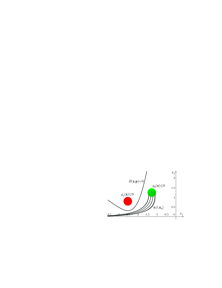
Figure 3: Results for Example 5.1.

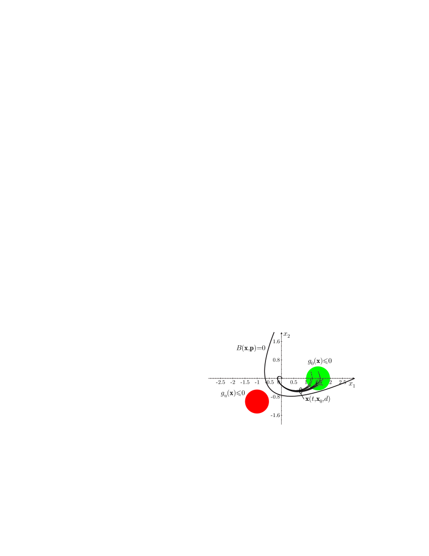
Figure 4: Results for Example 5.4 with various values of the disturbance $d$.

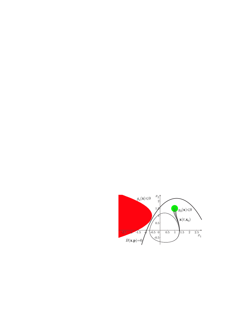
Figure 5: Results for Example 5.5.

The results in Table 1 show the importance of contractors which are beneficial in all cases. Thanks to contractors, valid barrier functions were obtained for all examples, which is not the case employing the original version of CSC-FPS proposed in [18]. In theory, both FPS and CSC are of exponential complexity in the dimension $m$ of the parameter space and $n$ of the state space. In practice, contractors allow, on the considered examples, to break this complexity and to consider high-dimensional problems.

The search for barrier functions using the relaxed version (14) of the constraint (12) as in [24], has also been performed using the version of our algorithms with contractors considering the same parametric barrier functions. We were not able to find a valid barrier function in less than $30$ minutes. This shows the detrimental effect of the relaxation (14) on the search technique.

Some examples were also addressed using RSolver, which is a tool to solve some classes of QCSP [25]. Nevertheless, this requires some modifications of the examples, since RSolver does not address dynamics or constraints involving divisions [26]. Moreover, the type of constraints processed by RSolver, for problems such as (20), allows only parametric barrier functions that are linear in the parameters. Outer-approximating boxes for the initial and the unsafe regions $\mathcal{X}_{0}$, $\mathcal{X}_{u}$ defined by $g_{0}$ and $g_{u}$ are given to Rsolver. As a consequence, Examples 5.1, 5.2 and 5.3 could not be considered. Only Examples 5.4, 5.5, and 5.6 were tested by Rsolver, which was able to find a satisfying barrier function only for Lorenz in less than $1$s. RSolver was unable to find a solution for Examples 5.4 and 5.5. Rsolver is well designed for problems with parametric barriers linear in the parameters, but has difficulties for non-linear problem and non-convex constraints such as (12).

Table 1: Results of CSC-FPS without and with contractors

			Without contr.		With contr.
Example	$n$	$m$	time	bisect.	time	bisect.
1	2	4	$36$s	$4520$	$16$s	$4553$
2	2	3	T.O.	/	$1$s	$159$
3	2	6	$1133$s	$20388$	$1$s	$6$
4	2	6	$253$s	$14733$	$7$s	$435$
5	2	4	T.O.	$/$	$98$s	$4072$
6	3	4	$167$s	$1753$	$21$s	$47$
7	6	7	$697$s	$67600$	$1$s	$261$

6 Conclusion

This paper presents a new method to find parametric barrier functions for nonlinear continuous-time perturbed dynamical systems. The proposed technique has no restriction regarding the dynamics nor the form of the barrier function. The search for barrier functions is formulated as an interval quantified constraint statisfaction problem. A branch-and-prune algorithm proposed in [18] has been supplemented with contractors to address this problem. Contractors are instrumental in solving problems with large number of parameters. The proposed approach can thus find barrier functions for a large class of possibly perturbed dynamical systems.

Alternative techniques based on RSolver may be significantly more efficient for some specific classes of problems where the parameters appear linearly in the parametric barrier functions. A combination of RSolver and our approach may be useful to improve the global efficiency of barrier function caracterization.

Future work will be dedicated to the search for the class of parametric barrier functions to consider. This may be done by exploring a library of candidate barrier functions. In our approach rejection of a candidate function occurs mainly after a timeout. Even if contractors aiming at eliminating some parts of the parameter space were defined, their efficiency is limited. Better contractors for that purpose may be very helpful.

An other future research direction is to extend the proposed method to hybrid systems as done in [24], i.e., to consider a set of quantified constraints for each location of an hybrid automaton and the constraints associated to the transitions.

References

- [1] Mathcurve. http://www.mathcurve.com/.
- [2] A. A. Ahmadi, M. Krstic, and P. A. Parrilo. A globally asymptotically stable polynomial vector field with no polynomial Lyapunov function. In Proc. of CDC-ECE, pages 7579–7580, 2011.
- [3] I. Araya, G. Trombettoni, B. Neveu, and G. Chabert. Upper bounding in inner regions for global optimization under inequality constraints. Journal of Global Optimization, vol. 60(2):145–164, 2012.
- [4] E. Asarin, O. Bournez, T. Dang, and O. Maler. Approximate reachability analysis of piecewise-linear dynamical systems. In Proc. Hybrid Systems: Computation and Control, pages 20–31. Springer, 2000.
- [5] R. E. Bellman and K. L. Cooke. Differential-difference equations. RAND Corporation, 1963.
- [6] F. Benhamou and F. Goualard. Universally quantified interval constraints. In Proc. Principles and Practice of Constraint Programming, pages 67–82. Springer, 2000.
- [7] G. Chabert and L. Jaulin. Contractor programming. Artificial Intelligence, 173(11):1079–1100, 2009.
- [8] X. Chen, E. Abrahám, and S. Sankaranarayanan. Taylor model flowpipe construction for non-linear hybrid systems. In Proc. IEEE Real-Time Systems Symposium, pages 183–192, San Juan (Porto Rico), 2012.
- [9] A. Chutinan and B. H. Krogh. Verification of polyhedral-invariant hybrid automata using polygonal flow pipe approximations. In Proc. Hybrid Systems: Computation and Control, pages 76–90. Springer, 1999.
- [10] A. Chutinan and B. H Krogh. Computational techniques for hybrid system verification. on IEEE trans. Autom. Control, 48(1):64–75, 2003.
- [11] G. Frehse, C. Le Guernic, A. Donzé, S. Cotton, R. Ray, O. Lebeltel, R. Ripado, A. Girard, T. Dang, and O. Maler. Spaceex: Scalable verification of hybrid systems. In Computer Aided Verification, pages 379–395. Springer, 2011.
- [12] J. H. Gallier. Logic for computer science. Longman Higher Education, 1986.
- [13] R. Genesio, M. Tartaglia, and A. Vicino. On the estimation of asymptotic stability regions: State of the art and new proposals. Trans. Autom. Control, 30(8):747–755, 1985.
- [14] A. Girard, C. Le Guernic, and O. Maler. Efficient computation of reachable sets of linear time-invariant systems with inputs. In Proc. Hybrid Systems: Computation and Control, pages 257–271. Springer, 2006.
- [15] H. Guéguen and J. Zaytoon. On the formal verification of hybrid systems. Control Engineering Practice, 12(10):1253 – 1267, 2004.
- [16] S. Gulwani and A. Tiwari. Constraint-based approach for analysis of hybrid systems. In Computer Aided Verification, pages 190–203. Springer, 2008.
- [17] L. Jaulin, M. Kieffer, O. Didrit, and É. Walter. Applied Interval Analysis. Springer, 2001.
- [18] L. Jaulin and É. Walter. Guaranteed tuning, with application to robust control and motion planning. Automatica, 32(8):1217–1221, 1996.
- [19] J. Lygeros, C. Tomlin, and S. Sastry. Controllers for reachability specifications for hybrid systems. Automatica, 35(3):349–370, 1999.
- [20] A. Papachristodoulou and S. Prajna. On the construction of lyapunov functions using the sum of squares decomposition. In Proc CDC, volume 3, pages 3482–3487, 2002.
- [21] A. Papachristodoulou and S. Prajna. Analysis of non-polynomial systems using the sos decomposition. In Positive Polynomials in Control, pages 23–43. Springer, 2005.
- [22] P. A. Parrilo. Semidefinite programming relaxations for semialgebraic problems. Mathematical programming, 96(2):293–320, 2003.
- [23] S. Prajna. Barrier certificates for nonlinear model validation. Automatica, 42(1):117–126, 2006.
- [24] S. Prajna and A. Jadbabaie. Safety verification of hybrid systems using barrier certificates. In Proc. Hybrid Systems: Computation and Control, pages 477–492. Springer, 2004.
- [25] S. Ratschan. Efficient solving of quantified inequality constraints over the real numbers. ACM Trans. on Computational Logic, 7(4):723–748, 2006.
- [26] S. Ratschan. Rsolver user manuel. http://rsolver.sourceforge.net, 2007.
- [27] S. Ratschan and Z. She. Providing a basin of attraction to a target region by computation of Lyapunov-like functions. In Proc IEEE International Conference on Computational Cybernetics, pages 1–5, 2006.
- [28] S. Sankaranarayanan, H. B. Sipma, and Z. Manna. Constructing invariants for hybrid systems. In Proc. Hybrid Systems: Computation and Control, pages 539–554. Springer, 2004.
- [29] Z. Sun, S. S. Ge, and T. H. Lee. Controllability and reachability criteria for switched linear systems. Automatica, 38(5):775–786, 2002.
- [30] A. Tiwari. Approximate reachability for linear systems. In Proc. Hybrid Systems: Computation and Control, pages 514–525. Springer, 2003.
- [31] C. Tomlin, G. J. Pappas, and S. Sastry. Conflict resolution for air traffic management: A study in multiagent hybrid systems. IEEE Trans on Automatic Control, 43(4):509–521, 1998.
- [32] A. Vaněček and S. Čelikovskỳ. Control systems: from linear analysis to synthesis of chaos. Prentice Hall Hertfordshire (UK), 1996.