The free energy cost of accurate biochemical oscillations

Abstract

Oscillation is an important cellular process that regulates timing of different vital life cycles. However, in the noisy cellular environment, oscillations can be highly inaccurate due to phase fluctuations. It remains poorly understood how biochemical circuits suppress phase fluctuations and what is the incurred thermodynamic cost. Here, we study four different types of biochemical oscillations representing three basic oscillation motifs shared by all known oscillatory systems. We find that the phase diffusion constant follows the same inverse dependence on the free energy dissipation per period for all systems studied. This relationship between the phase diffusion and energy dissipation is shown analytically in a model of noisy oscillation. Microscopically, we find that the oscillation is driven by multiple irreversible cycles that hydrolyze the fuel molecules such as ATP; the number of phase coherent periods is proportional to the free energy consumed per period. Experimental evidence in support of this universal relationship and testable predictions are also presented.

I introduction

Living systems are dissipative, consuming energy to perform key functions for their survival and growth. While it is clear that free energy EisenbergHill1985 ; Hill2005 ; QianBeard2008 is needed for physical functions, such as cell motility Julicher1997 and macromolecule synthesis Nelson2008 , it remains poorly understood whether and how regulatory functions are enhanced by free energy consumption. The relationship between biological regulatory functions and nonequilibrium thermodynamics has been an active area in biophysics BialekSetayeshgar2005 ; HuChen2010 ; LanSartori2012 ; LanTu2013 ; SkogeNaqvi2013 ; LangFisher2014 . For example, recent studies in different cellular adaptation processes demonstrated that the cost-performance trade-off follows a universal relationship, independent of the detailed biochemical circuits LanSartori2012 ; LanTu2013 .

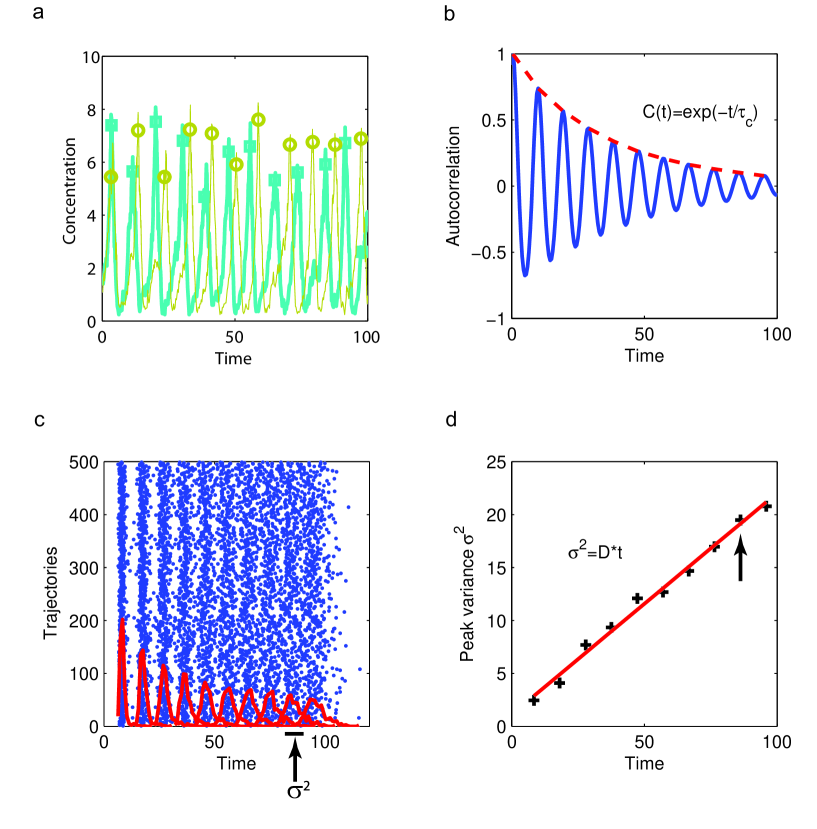
Figure 1: Correlation and phase diffusion in the activator-inhibitor model with $V=50,\gamma=10^{-5}$. (a) Two noisy oscillation trajectories, with the peaks labeled by circles and squares. (b) Auto-correlation function (defined in Eq. 1) of the inhibitor $X$. $C(t)$ decays exponentially with correlation time $\tau_{c}=37.7$. (c) Raster plot of the peak times for $500$ different trajectories starting with the same initial condition. The distributions of the peak times for each consecutive peaks are shown by red lines. The peak time variance $\sigma^{2}$ is shown. (d) Peak time variance $\sigma^{2}$ goes linearly with the average peak time, with the linear coefficient defined as the peak time diffusion constant. Here, the diffusion constant $D=0.2$ and $\alpha\equiv\tau_{c}D/T^{2}\approx 0.07$.

Oscillatory behaviors exist in many biological systems, e.g., glycolysis Goldbeter1996 , cyclic AMP signaling MartielGoldbeter1987 , cell cycle Pomerening2003 ; Tsai2008 ; FerrellTsai2011 , circadian rhythms Goldbeter1996 ; HogeneschUeda2011 , and synthetic oscillators ElowitzLeibler2000 ; Stricker2008 . These biochemical oscillations are crucial in controlling the timing of life processes. Much is known now about the structure of biochemical circuits responsible for these oscillatory behaviors. There are a few basic network motifs, illustrated in Figure 1a, which are responsible for all known biochemical and genetic oscillations Goldbeter1996 ; MartielGoldbeter1987 ; FerrellTsai2011 ; HogeneschUeda2011 ; ElowitzLeibler2000 . These network motifs share a few essential features, such as nonlinearity, negative feedback, and a time delay, as summarized by Novak and Tyson in NovakTyson2008 . However, in small systems such as a single cell, the dynamics of oscillations are subject to large fluctuations from the environment, due to their small sizes. Thus, one may ask how biological systems maintain coherence of oscillations amidst these fluctuations BarkaiLeibler2000 . Here, we study the thermodynamic cost of controlling oscillation coherence in different representative oscillatory systems and investigate whether there is a general (universal) relation between the accuracy of the oscillation and its minimum free energy cost that may apply to all biochemical oscillations.

We study four specific models, the activator-inhibitor (AI) model, the repressilator model, the brusselator model, and the allosteric glycolysis model, chosen to exemplify the three different basic oscillation motifs, as shown in Fig. 1. For all the systems studied, a finite (critical) amount of free energy is needed to drive them to oscillate. Beyond the onset of oscillation, extra free energy dissipation is used to reduce the phase diffusion constant and thus enhance the coherence time and phase accuracy of the oscillations. A general inverse relationship between the phase diffusion constant and the free energy dissipation is found in all the four models studied, suggesting that the relation may hold true for all biochemical oscillations. The energy-accuracy relation for noisy oscillations is also verified analytically in the noisy complex Stuart-Landau equation. In the following, we report these results followed by a in-depth discussion of a plausible general microscopic mechanism/strategy for energy-assisted noise suppression.

II models and results

II.1 Four biochemical oscillators representing the basic network motifs

All known biochemical and genetic oscillators contain at least one of the basic motifs (or their variance) in network topology NovakTyson2008 ; vanDorp2013. To search for general principles in these noisy oscillatory systems, we study four biochemical systems (Fig. References), each representing one of the three basic network motifs responsible for oscillatory behaviors. The first one is the activator-inhibitor (AI) system, where a negative feedback is interlinked with a positive feedback (Left panel, Fig. 1a). This regulatory motif is common in biological oscillators, like the circadian clock in cyanobacteria Nakajima2005 ; RustMarkson2007 , cell cycle in frog egg Goldbeter1991 ; Pomerening2005 , cAMP signaling in Dictyostelium, and genetic oscillators in synthetic biology Stricker2008 ; DaninoMondragon-Palomino2010 ; Prindle2012 . We implement this motif in a simplified biological network with a phosphorylation-dephosphorylation cycle (Fig. 1b). The second model is a repressilator, which consists of three components connected in a negative feedback loop, such that each component represses the next one in the loop, and is itself repressed by the previous one (Middle panel, Fig. 1a). The first synthetic genetic oscillator was built with this motif ElowitzLeibler2000 . Many important transcriptional-translational oscillators also use this motif as their backbone, such as circadian clock in mammalian cells HogeneschUeda2011 , NF-$\kappa$B signaling KrishnaJensen2006 , and the p53-mdm2 oscillations in cancer cells Geva-ZatorskyRosenfeld2006 . Here, we take the repressilator composed of CDK1, Plk1, and APC in a cell cycle as our case study (Fig. 1c). The third model we chose is the brusselator, which is one of the simplest two-component systems that can generate sustained oscillations (Right panel, Fig. 1a). The concentration fluctuations due to small molecule numbers were analyzed in QianSaffarian2002 , here, we aim to study the effect of noise on the phase of the oscillation. The brusselator (Fig. 1d) is a special kind of substrate-depletion model SzallasiStelling2006 , where substrate $S$ is converted by a process that is amplified autocatalytically by the product $P$. Examples of substrate-depletion motif are oscillations in glycolysis GoldbeterLefever1972 ; Goldbeter1996 and Calcium signaling Dupont1991 . Here, we examine the noise effect in glycolysis oscillations, where the allosteric enzyme PFK catalyzes substrate to product in a network shown in Fig. 1e.

In our study, we introduced a parameter $\gamma$ to characterize the reversibility of the biochemical networks. In a reaction loop, $\gamma$ corresponds to the ratio of the product of the reaction rates in one direction (e.g., counter-clock-wise) and that in the other direction (e.g., clock-wise). When $\gamma=1$, the system is in equilibrium without any free energy dissipation. For $\gamma\neq 1$, free energy is dissipated. Here, we study the relationship between the dynamics and the energetics of the biochemical networks by varying $\gamma$. The mathematical details of the four models are described in the Supplemental Information (SI), all parameters (e.g., reaction rates, concentrations, time, and volumes) are shown here as dimensionless numbers with their units explained in SI.

II.2 Phase diffusion reduces the coherence time

In all four models that we studied, there is an onset of oscillation as $\gamma$ decreases below a critical value $\gamma_{c}\;(<1)$. This means that a finite critical free energy dissipation ($W_{c}>0$) is needed to generate an oscillatory behavior (see Fig. S1 in SI). In Fig. 2a, two trajectories of the concentration of the inhibitor $X$ are shown for $\gamma<\gamma_{c}$ in the activator-inhibitor model, where $\gamma_{c}=2\times 10^{-3}$. As evident in Fig. 2a, biochemical oscillations are noisy. To characterize the coherence of the oscillation in time, we computed the auto-correlation function $C(t)$ for a given concentration variable $x$ in the network. As shown in Fig. 2b, $C(t)$ follows a damped oscillation:

$$C(t)\equiv\frac{\langle(x(t+s)-\langle x\rangle)(x(s)-\langle x\rangle)\rangle_{s}}{\langle x^{2}\rangle-\langle x\rangle^{2}}=\exp(-t/\tau_{c})\times\cos(2\pi t/T),$$ (1)

where $T$ is the period and $\tau_{c}$ defines a coherence time for the oscillation.

The oscillatory state breaks time translation invariance (symmetry) of the underlying biochemical system. As a result, the phase of the oscillation is a soft mode and follows diffusive dynamics in the presence of noise. To quantify the phase diffusion, we simulated many trajectories in the model(s) with the same parameters and the same initial conditions. In Fig. 2c, the peak times for $500$ trajectories in the AI model are shown in a raster plot together with the peak time distributions (red lines). The variance ($\sigma^{2}$) of the distribution versus the average peak time is shown in Fig. 2d. It is clear that the variance goes linearly with time, confirming the diffusive nature of the phase, and the linear slope defines a peak time diffusion constant $D$. It is easy to show that the coherence time $\tau_{c}$ is inversely proportional to $D$:

$$\tau_{c}=\alpha T^{2}/D,$$ (2)

where $\alpha$ is a constant dependent on the waveform ($\alpha=(2\pi^{2})^{-1}$ for a sine wave).

II.3 Free energy dissipation suppresses phase diffusion

As $\gamma$ decreases below $\gamma_{c}$, more free energy is dissipated. What is the effect of the additional free energy dissipation beyond the onset of oscillation? From the chemical reaction rates, we can compute the free energy dissipation rate Qian2007 :

$$\dot{W}=\sum_{i}(J_{i}^{+}-J_{i}^{-})\ln{\frac{J_{i}^{+}}{J_{i}^{-}}}$$ (3)

where $J_{i}^{+}$ and $J_{i}^{-}$ are the forward and backward fluxes of the $i$th reaction, and free energy is in units of $k_{B}T$, set to unity here. For the activator-inhibitor and glycolysis models, we calculated the energy dissipation rate using Eq. 3. For systems with continuum stochastic dynamics described by Langevin equations (e.g., the brusselator and the repressilator models), we can obtain the steady-state distribution $P(\vec{x})$ by solving the corresponding Fokker-Planck equation or by direct stochastic simulations (see Fig. S2 in SI for an example). From $P(\vec{x})$, we computed the phase space fluxes and the free energy dissipation rate following LanTu2013 (see the Methods section and SI for details). For oscillatory systems, the dissipation rate $\dot{W}$ varies in a period $T$. We define $\Delta W\equiv\int_{0}^{T}\dot{W}dt$ to characterize the free energy dissipation per period per volume.

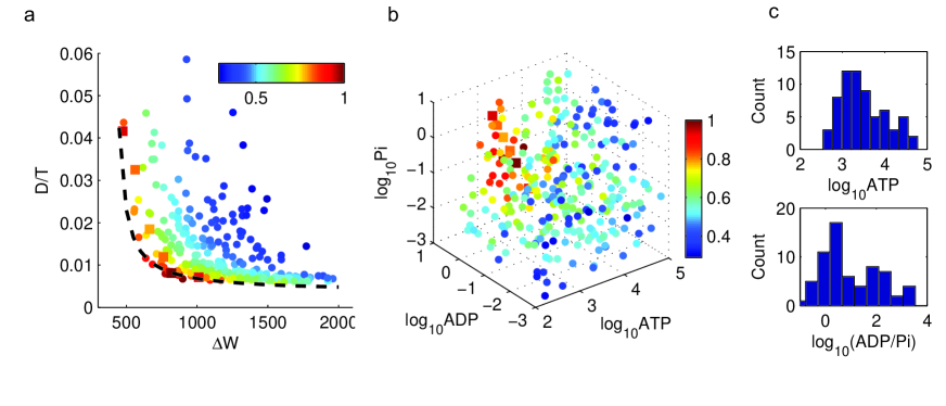
Figure 3: The dependence of phase diffusion on the ATP, ADP, and $P_{i}$ concentrations. We studied the activator-inhibitor model with $300$ randomly chosen parameters of dimensionless [ATP],[ADP] and $[P_{i}]$ (see Methods). The affected kinetic rates are $a_{1}=a_{1,0}[ATP],f_{-1}=f_{-1,0}[ADP],f_{-2}=f_{-2,0}[P_{i}]$ with $a_{1,0}=0.1,f_{-1,0}=f_{-2,0}=1$. We chose $V=100$. (a) $D/T$ versus $\Delta W$ for the $300$ different parameter choices. All the points lie above an envelope curve, which follows Eq. 4 with $D/T=1.94/(\Delta W-400)+0.0036$. Points in square indicate the points shown in Fig. 3. For a given value of $D/T$, the corresponding minimal energy dissipation $\Delta W_{min}$ is computed according to the fitted envelope curve. The efficiency is defined as $E\equiv\Delta W_{min}/\Delta W$. Colors of the points indicate the efficiency. (b) Distribution of the $300$ randomly sampled points in the parameter space $([ATP],[ADP],[P_{i}])$. Colors of the points indicate the efficiency as in (a). Points with high efficiency are clustered. (c) Distribution of [ATP], and [ADP]/[Pi] for parameter choices with high efficiency $E\geq 0.75$. The most probable parameter values for high efficiency are $[ATP]\approx 10^{3},[ADP]\approx[P_{i}]$, which corresponds to $a_{1}=a_{2},f_{-1}=f_{-2}$ in the kinetic equations. This result indicates that high efficiency is achieved when the kinetic rates in the two halves of the PdP cycle (phosphorylation and dephosphorylation) are matched.

For each of the four models, $\Delta W$ and the dimensionless peak time diffusion constant $D/T$ were computed for different parameter values (reaction rates, protein concentrations) in the oscillatory regime $\gamma<\gamma_{c}$ and for different volume $V$. As shown in Fig. 3, for all the four models considered, $D/T$ decreases as the energy dissipation $\Delta W$ increases and eventually saturates to a fixed value when $\Delta W\rightarrow\infty$ (i.e., $\gamma=0$). The phase diffusion constants scale inversely with the volume $V$. As shown in the insets of Fig. 3, the scaled $D/T$ (by the volume $V$) collapsed onto a simple curve, which can be approximated by the same simple form in all the four models studied:

$$V\times\frac{D}{T}\approx C+\frac{W_{0}}{\Delta W-W_{c}},$$ (4)

where $W_{c}$ is the critical free energy, and $W_{0}$ and $C$ are intensive constants (independent of volume), whose values in different systems (models) are given in the legend of Fig. 3.

II.4 The free energy sources and experimental evidence

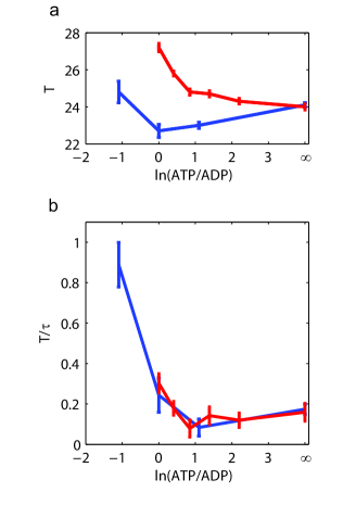
Figure 4: Experimental evidence from Ref.Phong2013 (blue curve) and Ref.Rust2011 (Red curve). The two experiments measured the oscillation of KaiC phosphorylation in vitro in media with different ATP/ADP ratios. The autocorrelation functions were calculated from the original data and fitted by a exponential decay cosine function $A\cos{(2\pi t/T)}e^{-t/\tau_{c}}$, where $T$ is the period, and $\tau_{c}$ is the correlation time. $\ln(ATP/ADP)$ represents the entropic contribution to the free energy. (a) The period $T$ is robust against changes in the ATP/ADP ratio. (b) $T/\tau_{c}\equiv\alpha^{-1}D/T$ decreases with $\ln(ATP/ADP)$ and eventually saturates at large ATP/ADP ratio, consistent with our theoretical prediction.

What is the free energy source driving the biochemical oscillations? For the activator-inhibitor model, the free energy is provided by ATP hydrolysis in the phosphorylation-dephosphorylation (PdP) cycle (see Fig. 1a). Besides the standard free energy $\Delta G_{0}$ of ATP hydrolysis, the total free energy dissipation per period $\Delta W$ also depends on (and thus can be controlled by) the concentrations of ATP, ADP and the inorganic phosphate $P_{i}$. These concentrations ([ATP], [ADP], and $[P_{i}]$) directly affect the biochemical reaction rates in our model and consequently the phase diffusion of the oscillation. In Fig. 4a, we show the phase diffusion constant ($D/T$) versus the dissipation per period ($\Delta W$) for $300$ randomly chosen points in the oscillatory regime of the ($[ATP]$, $[ADP]$, $[P_{i}]$) space (see Fig. 4b). Remarkably, all the points lie above an envelope curve (the dotted line), which follows Eq.3. This envelope curve defines the best performance of the biochemical network, i.e., the minimum free energy $\Delta W_{m}$ needed to achieve a given level of phase coherence. For each choice of the concentrations $([ATP],[ADP],[P_{i}])$, a functional efficiency $E$ can be defined as the ratio of $\Delta W_{m}$ and the actual cost $\Delta W$ for the same performance ($D/T$). The efficiency is represented by color in Fig. 4a&b. We investigated how efficiency depends on the three concentrations. As shown in Fig. 4c, the efficiency $E$ does not simply increase with the ATP concentration; instead it peaks near a particular level of [ATP], at which the phosphorylation and dephosphorylation fluxes are matched. Similarly, $E$ does not have any clear dependence on $[ADP]$ or $[P_{i}]$ level, it is high near a fixed ratio of $[ADP]/[P_{i}]$, when the kinetic rates of the phosphorylation and dephosphorylation parts of the PdP cycle are matched.

These predicted dependence of oscillatory behaviors on [ATP], [ADP], and $[P_{i}]$ concentrations, as shown in Fig. 4, may be tested experimentally by measuring peak-to-peak time variations or equivalently the correlation time for different nucleotide concentrations. As reported in two recent studies Rust2011 ; Phong2013 , the oscillatory dynamics of the phosophorylated KaiC protein in a reconstituted circadian clock from cyanobacteria (the Kai system) have been measured in media with different ATP/ADP ratios. We analysed the data according to Eq. 1 and obtained the correlation time ($\tau_{c}$) and the period ($T$) for different ATP/ADT ratios (see SI and Fig. S3 in SI for details). In Fig. 4, we plotted the period and the phase diffusion versus $\ln([ATP]/[ADP])$, which is the entropic contribution to the free energy dissipation. As the ATP/ADP ratio increases, the period changes little. In contrast, the phase diffusion $T/\tau_{c}\equiv\alpha^{-1}D/T$ decreases significantly and eventually saturates at high ATP/ADP ratios, consistent with the relationship between energy dissipation and phase diffusion discovered here.

II.5 Analytical results from the noisy Stuart-Landau equation

To understand the relationship between phase accuracy and energy dissipation, we consider the noisy Stuart-Landau equation for a complex order parameter $Z$:

$$\frac{dZ}{dt}=(a+ib)Z-(c+id)|Z|^{2}Z+\eta_{Z},$$ (5)

where $a$, $b$, $c(>0)$, $d$ are real variables, $i=\sqrt{-1}$, and $\eta_{Z}$ is a complex noise term. For $a>0$, the system starts to oscillate with a mean amplitude $r_{s}=\sqrt{\frac{a}{c}}$. Eq. (5) can be decomposed into two Langevin equations for the amplitude $r$ and the phase $\theta$ of $Z=re^{i\theta}$:

$$\frac{dr}{dt}=ar-cr^{3}+\eta_{r}(t)\;\;,\;\;\frac{d\theta}{dt}=b-dr^{2}+\eta_{\theta}(t),$$ (6)

where $\eta_{r}$ and $\eta_{\theta}$ are the white noises of the amplitude and the phase. For simplicity, we consider the case where $\eta_{r}$ and $\eta_{\theta}$ are uncorrelated with constant strength $\Delta_{r}$ and $\Delta_{\theta}$ respectively. The average phase velocity is $\omega(r)\equiv\langle d\theta/dt\rangle=b-dr^{2}$.

It is clear from Eq. 6 that detailed balance is broken and the system is dissipative. To compute the free energy dissipation, we first determine the phase-space probability distribution function $P(r,\theta,t)$, which follows the Fokker-Planck equation:

$$\frac{\partial{P}}{\partial{t}}=-\frac{1}{r}\frac{\partial}{\partial r}\big{[}(ar^{2}-cr^{4})P-\frac{\Delta_{r}r}{2}\frac{\partial P}{\partial r}\big{]}-\frac{\partial}{\partial\theta}\big{[}(b-dr^{2})P-\frac{\Delta_{\theta}}{2}\frac{\partial P}{\partial\theta}\big{]}\equiv-\frac{1}{r}\frac{\partial(rJ_{r})}{\partial r}-\frac{\partial J_{\theta}}{\partial\theta},$$ (7)

where $J_{r}$ and $J_{\theta}$ are the probability density fluxes in phase space. Since $\omega(r)$ does not depend on $\theta$, the steady state probability distribution $P_{s}(r,\theta)$ only depends on $r$:

$$P_{s}(r,\theta)=P(r)=A\exp{[-\frac{2(cr^{4}/4-ar^{2}/2)}{\Delta_{r}}]}$$ (8)

where $A=\big{[}2\pi\int{\exp{[-2(cr^{4}/4-ar^{2}/2)/\Delta_{r}]}rdr}\big{]}^{-1}$ is the normalization constant. From Eq. 8, the flux vanishes in the $r$-direction $J_{r}=0$. However, there is a finite flux in the $\theta$-direction $J_{\theta}(r)=\omega(r)P(r)$. We compute the system’s entropy production rate $\dot{S}$ Tomede-Oliveira2010 ; Seifert2005 , from which we obtain the minimum free energy dissipation (see SI for details):

$$\dot{W}=k_{B}T_{e}\int\int[\frac{J_{r}^{2}}{\Delta_{r}P}+\frac{J_{\theta}^{2}}{\Delta_{\theta}P}]rdrd\theta=k_{B}T_{e}\frac{\langle\omega^{2}\rangle}{\Delta_{\theta}},$$ (9)

where $T_{e}$ is an (effective) temperature of the environment, we set $k_{B}T_{e}=1$ here.

The phase diffusion constant is determined by expanding the phase velocity $\omega(r)$ around $r=r_{s}$, the most probable amplitude from $P(r)$. This leads to $d\theta/dt=\omega(r_{s})+\beta\delta r(t)+\eta_{\theta}(t)$, with $\beta\equiv\partial\omega(r_{s})/\partial r=-2d\sqrt{a/c}$. The period of the oscillation is $T=2\pi/\omega(r_{s})$, and the phase fluctuation $\delta\theta\equiv\theta-\omega(r_{s})t$ follows diffusion with the diffusion constant given by:

$$D_{\theta}=\frac{\beta^{2}\Delta_{r}}{4a^{2}}+\Delta_{\theta}.$$ (10)

From Eq. 9&10, the relation between phase diffusion and energy dissipation emerges:

$$D_{\theta}=D_{0}+\frac{\langle\omega^{2}\rangle T}{\Delta W}\equiv C+\frac{W_{0}}{\Delta W-W_{c}},$$ (11)

where $W_{c}=0$ because $J_{r}=0$, something that is not generally valid (see SI and Fig. S4 in SI for a more general case of the noisy Stuart-Landau equation). The two constants, $C=D_{0}=\frac{\beta^{2}\Delta_{r}}{4a^{2}}$ and $W_{0}=\langle\omega^{2}\rangle T$, depend on the details of the system.

Eq.11 has the same form as Eq. 4 obtained empirically from studying different biochemical networks. Analysis of the noisy Stuart-Landau equation clearly shows that free energy dissipation is used to suppress phase diffusion to increase the coherence of the oscillation. Though parameters in this relation may depend on the details of the system, the inverse dependence of phase diffusion on energy dissipation appears to be universal.

III discussion

Oscillations are critical for many biological functions that require accurate time control, such as circadian clock, cell cycle, and development. However, biological systems are inherently noisy. The phase of a noisy oscillator fluctuates (diffuses) without bound and eventually destroys the coherence (accuracy) of the oscillation. Specifically, the number of periods $N_{c}$ in which the oscillation maintains its phase coherence is given by $N_{c}=\tau_{c}/T=\alpha T/D$, which decreases with the phase diffusion constant. Here, our study shows that free energy dissipation can be used to reduce phase diffusion and thus prolong the coherence of the oscillation. A general relationship between the phase diffusion constant and the minimum free energy cost, as given in Eq. 4, holds true for all the oscillatory systems we studied here. The amplitude fluctuations also decrease with free energy dissipation (see Fig. S5 in SI for details), as fluctuations in phase and amplitude are coupled in realistic systems. Our study thus establishes a cost-performance tradeoff for noisy biochemical oscillations.

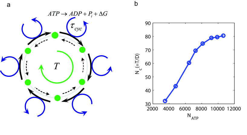
Figure 5: Oscillation coherence increases with the number of ATP hydrolyzed per period. (a) Illustration of a biochemical oscillation as a clock in phase space. The intermediate states (green dots) are represented as the ”hour ticks” of the clock. The transition from one tick to the next is coupled with a ATP hydrolysis cycle. The free energy release $\Delta G$ from the hydrolysis cycle powers the forward transition (thick solid arrow) and/or suppresses the backward transition (thin dotted arrow). The number of ATP consumed per enzyme molecule in each period $T$ is given by $T/\tau_{cyc}$, where $\tau_{cyc}$ is the average cycle time. (b) The accuracy of the oscillation, characterized by the number of correlated (coherent) periods $N_{c}$, increases linearly with the total number of ATP consumed per period $N_{ATP}$ before saturating at very high $N_{ATP}$. We varied $N_{ATP}$ by changing the cycle time (see Methods for details), we used $V=100$ here.

How do biological systems use their free energy sources (e.g., ATP) to enhance the accuracy of the biochemical oscillations? As illustrated in Fig. 5a, a biochemical oscillation can be considered as a clock, which goes through a series of time-ordered chemical states (green dots) during each period. These chemical states are characterized by the conformational and chemical modification (e.g., phosphorylation) states of the key proteins or protein complexes in the system. The forward transition from one state to the next is coupled to a PdP cycle (blue arrowed circle) driven by hydrolysis of one ATP molecule. For each forward step, the reverse transition introduces a large error in the clock. The system suppresses these backward transitions by utilizing the ATP hydrolysis free energy. However, this is just one half of the story. Even in the absence of the reverse transition, the time duration between two consecutive states is highly variable due to the stochastic nature (Poisson process) of the chemical transitions. A general strategy of increasing accuracy is averaging bergpurcell. In the case of biochemical oscillations, each period may consist of multiple steps, each powered by at least one ATP molecule. As a result of averaging, the error in the period should go down as the number of steps increases. Specifically, we expect that the variance of the period $\sigma_{T}^{2}(=D/T)$ should be inversely proportional to the total number of ATP hydrolyzed $N_{ATP}\propto T/\tau_{cyc}$ in each period $T$, where $\tau_{cyc}$ is the average PdP cycle time, which is essentially the ATP turnover time. Consequently, the number of coherent period $N_{c}=\alpha T/D$ should be proportional to the number of ATP hydrolyzed in each period. We checked this prediction by varying the kinetic rates in the PdP cycle to change $\tau_{cyc}$ (see Methods section for details). In Fig. 5b, it is shown that the accuracy of the oscillation (clock), as measured by $N_{c}$, is enhanced by the number of ATP molecules hydrolyzed in each period. This result reveals a general strategy for oscillatory biochemical networks to enhance their phase coherence by coupling to multiple energy consuming cycles in each period. Interestingly, approximately $15$ ATP molecules are consumed per KaiC molecule per period in the circadian clock of cyanobacteria Terauchi2007 .

Biological systems need to function robustly against variations in its underlying biochemical parameters (rates, concentrations) BarkaiLeibler1997 ; MaTrusina2009 . For oscillatory networks, the free energy dissipation needs to reach a critical value ($W_{c}$) to drive the system to oscillate. We showed here that additional free energy cost in excess of $W_{c}$ is needed to make the oscillation more accurate, as demonstrated explicitly in Eq. 4. In addition to this accuracy-energy tradeoff, we found that larger energy dissipation can also enhance the system’s robustness against its parameter variations. Take the activator-inhibitor model, for example: the concentrations of enzyme E ($E_{T}$) and phosphatase K ($E_{K}$) may vary from cell to cell. We search for the existence of oscillation in the ($E_{T}$, $K_{T}$) space for different values of $\gamma$. Robustness is defined as the area of the parameter space where oscillation exists. As shown in Fig. S6 in the SI, the robustness increases as the system becomes more irreversible, i.e., when more free energy dissipation is dissipated. This suggests a possible general tradeoff between the functional robustness and energy dissipation in biological networks.

IV Acknowledgement

We thank Dr. Michael Rust for sharing the experimental data in Ref. Rust2011 &Phong2013 with us. This work is partly supported by a NIH grant (R01GM081747 to YT).

V Methods

Simulation Methods. The Gillespie algorithm Gillespie1977 is used for the stochastic simulations of the reaction kinetics. For given kinetic rates and the volume $V$, we simulated $1000$ trajectories starting with the same initial condition. For the $j$th trajectory, we obtained its $i$th peak time $t_{ij}$ from the trajectory $x_{j}(t)$ after smoothing (smooth function in MATLAB was used). The peak positions for two trajectories are shown in Fig. 2a. For all the trajectories, we computed the mean of their $i$th peak time $m_{i}=\sum_{j}t_{ij}/N$, and variance $\sigma^{2}_{i}=\sum_{j}(t_{ij}-m_{i})^{2}/(N-1)$, where $N$ is the total number of trajectories. The average period $T$ is given by $T=m_{i}/i$. Asymptotically, $\sigma_{i}^{2}$ depends linearly on $m_{i}$ (Fig. 2d), and the slope of this linear dependence is the peak time diffusion constant $D$, which has the dimension of time. The phase diffusion constant $D_{\phi}$ is linearly proportional to $D$: $D_{\phi}=(2\pi)^{2}D/T$. For the repressilator and the brusselator models, we simulated the stochastic kinetic equations to a sufficiently long time ($10000$ periods) to obtain the time-averaged distribution $P(\vec{x})$, where $\vec{x}$ represents the phase space. We used $P(\vec{x})$ to compute free energy dissipation.

Random Sampling in the $([ATP],[ADP],[P_{i}])$ space is performed (in log scale) in the region $\log_{10}\frac{[ATP]}{[ATP]_{0}}\in[2,5],\log_{10}\frac{[ADP]}{[ADP]_{0}}\in[-3,1],\log_{10}\frac{[P_{i}]}{[P_{i}]_{0}}\in[-3,1]$ by using Latin hypercube sampling (the lhsdesign function in MATLAB). The reference concentrations $[ATP]_{0}$, $[ADP]_{0}$, and $[P_{i}]_{0}$ are set to unity and their actual values are absorbed into the baseline reaction rates $a_{1,0}$, $f_{-1,0}$ and $f_{-2,0}$, which are given in the legend of Fig. 4.

ATP consumption. In the activator-inhibitor model, the ATP consumption rate is $R_{ATP}=V(J_{p}^{+}-J_{p}^{-})$, where $J_{p}^{+}$ and $J_{p}^{-}$ are the fluxes for the $E\rightarrow E_{p}$ and $E_{p}\rightarrow E$ reactions, respectively. We varied the overall reaction kinetics, e.g., $\tau_{cyc}$ and the ATP consumption rate, by introducing a timescale factor $B$ for all four rates $d_{1}=d_{2}=Bd,f_{1}=f_{2}=Bf$, where $d=15,f=15$ are the original values used in this paper (see SI). By changing the rates this way, the free energy release of ATP hydrolysis $\Delta G=-\ln{\gamma}=\ln(a_{1}f_{1}a_{2}f_{2}/(d_{1}f_{-1}d_{2}f_{-2}))$ is unchanged. We varied $B\in[0.2,2]$, and computed the total number of ATP consumed per period $N_{ATP}\equiv\int_{0}^{T}R_{ATP}dt$ and $N_{c}$ for Fig. 5b.

VI Acknowledgement

We thank Dr. Michael Rust for sharing the experimental data in Ref. Rust2011 &Phong2013 with us. This work is partly supported by a NIH grant (R01GM081747 to YT).

Different network motifs and the corresponding biochemical oscillatory systems. (a) Illustrations of three network motifs for oscillation: activator-inhibitor, repressilator, and substrate-depletion. (b) The activator-inhibitor model with a phosphorylation-dephosphorylation (PdP) cycle. R and K catalyse two opposing reactions $E\leftrightarrow E_{p}$ (phosphorylation and dephosphorylation) through different intermediate complexes $ER$ and $E_{p}K$. $E_{p}$ activates both $R$ (activator) and $X$ (inhibitor). $X$ inhibits $R$ by enhancing its degradation. Parameter $\gamma=d_{1}f_{-1}d_{2}f_{-2}/(a_{1}f_{1}a_{2}f_{2})$ is introduced to characterize the reversibility of the system. (c) The “repressilator” model of cell cycle in eukaryotic cells. In the simplified network, CDK1 activates Plk1, Plk1 activates APC, and APC degrades CDK1 (dashed line), forming the mutually activing/inhibiting loop. Other intermediates are ignored here. (d) The brusselator model with detailed reactions. A and B are constant sources. (e) The glycolysis network. The allosteric enzyme’s protomer has two states, R (binding with P) and T (unbinding with P), and only R has the catalysis activity. Each $R_{i,j}$, with $i=1,2,\cdots,n_{i}$ and $j=1,2,\cdots,n_{j}$ represent the number of $S$ and $P$ bound to $R$, here we used $n_{i}=n_{j}=2$. Each $R_{i,j}$ can undergo reactions of $R_{i,j}+S\leftrightarrow R_{i,j+1}\leftrightarrow R_{i,j}+P$. Detailed descriptions and rate values are given in SI.

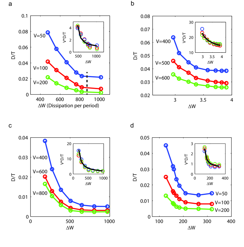
Figure 2: Relation between the dimensionless diffusion constant ($D/T$) and free energy dissipation per period per volume ($\Delta W$, in units of $k_{B}T$) for the four oscillatory systems. Detailed descriptions of the models and parameters can be found in SI. The relationships for different volumes collapse onto the same curve when the peak time diffusion constant is scaled by $V$, as shown in the insets. The black dashed line in the activator-inhibitor model indicates the value of $\Delta W$ if we assume that hydrolysis of one ATP molecule provides $\approx 12k_{B}T$ energy, which corresponds to $\gamma\approx 10^{-5.2}$. All the data can be well fitted with Eq. 4: $V\times D/T=C+W_{0}/(W-W_{c})$ (lines in insets), where $W_{c}$ is determined from the critical value $\gamma_{c}$, $W_{0}$ and $C$ are from fitting. The parameters are: (a) activator-inhibitor, $W_{c}=360.4,W_{0}=447.3\pm 55.8,C=0.28\pm 0.16$; (b) repressilator, $W_{c}=1.9,W_{0}=17.7\pm 3.9,C=5.5\pm 2.5$; (c) brusselator, $W_{c}=93.1,W_{0}=1135\pm 142,C=0.27\pm 0.11$; (d) glycolysis, $W_{c}=67.4,W_{0}=135.8\pm 3.4,C=0.025\pm 0.019$.

References

- (1) Eisenberg, E. & Hill, T. L. Muscle contraction and free energy transduction in biological systems. Science 227, 999–1006 (1985).
- (2) Hill, T. L. Free energy transduction and biochemical cycle kinetics (Academic Press, New York, 1977).
- (3) Qian, H. & Beard, D. A. Chemical biophysics :quantitative analysis of cellular systems. Cambridge texts in biomedical engineering (Cambridge University Press, Cambridge, 2008).
- (4) Jülicher, F., Ajdari, A. & Prost, J. Modeling molecular motors. Rev. Mod. Phys. 69, 1269 (1997).
- (5) Nelson, D. L., Lehninger, A. L. & Cox, M. M. Lehninger principles of biochemistry (Macmillan Publisher, New York, 2008).
- (6) Bialek, W. & Setayeshgar, S. Physical limits to biochemical signaling. Proc Natl Acad Sci U S A 102, 10040–5 (2005).
- (7) Hu, B., Chen, W., Rappel, W. J. & Levine, H. Physical limits on cellular sensing of spatial gradients. Phys Rev Lett 105, 048104 (2010).
- (8) Lan, G., Sartori, P., Neumann, S., Sourjik, V. & Tu, Y. The energy-speed-accuracy tradeoff in sensory adaptation. Nat Phys 8, 422–428 (2012).
- (9) Lan, G. & Tu, Y. The cost of sensitive response and accurate adaptation in networks with an incoherent type-1 feed-forward loop. J R Soc Interface 10, 20130489 (2013).
- (10) Skoge, M., Naqvi, S., Meir, Y. & Wingreen, N. S. Chemical sensing by nonequilibrium cooperative receptors. Phys Rev Lett 110, 248102 (2013).
- (11) Lang, A. H., Fisher, C. K., Mora, T. & Mehta, P. Thermodynamics of statistical inference by cells. Phys Rev Lett 113, 148103 (2014).
- (12) Goldbeter, A. Biochemical oscillations and cellular rhythms: the molecular bases of periodic and chaotic behaviour (Cambridge University Press, Cambridge, 1996).
- (13) Martiel, J. L. & Goldbeter, A. A model based on receptor desensitization for cyclic amp signaling in dictyostelium cells. Biophys J 52, 807–28 (1987).
- (14) Pomerening, J. R., Sontag, E. D. & Ferrell, J. E. Building a cell cycle oscillator: hysteresis and bistability in the activation of cdc2. Nature Cell Biology 5, 346–351 (2003).
- (15) Tsai, T. Y.-C. et al. Robust, tunable biological oscillations from interlinked positive and negative feedback loops. Science 321, 126–129 (2008).
- (16) Ferrell, J. J., Tsai, T. Y. & Yang, Q. Modeling the cell cycle: why do certain circuits oscillate? Cell 144, 874–85 (2011).
- (17) Hogenesch, J. B. & Ueda, H. R. Understanding systems-level properties: timely stories from the study of clocks. Nat Rev Genet 12, 407–16 (2011).
- (18) Elowitz, M. B. & Leibler, S. A synthetic oscillatory network of transcriptional regulators. Nature 403, 335–8 (2000).
- (19) Stricker, J. et al. A fast, robust and tunable synthetic gene oscillator. Nature 456, 516–519 (2008).
- (20) Novak, B. & Tyson, J. J. Design principles of biochemical oscillators. Nat Rev Mol Cell Biol 9, 981–91 (2008).
- (21) Barkai, N. & Leibler, S. Circadian clocks limited by noise. Nature 403, 267–8 (2000).
- (22) Nakajima, M. et al. Reconstitution of circadian oscillation of cyanobacterial kaic phosphorylation in vitro. Science 308, 414–415 (2005).
- (23) Rust, M. J., Markson, J. S., Lane, W. S., Fisher, D. S. & O’Shea, E. K. Ordered phosphorylation governs oscillation of a three-protein circadian clock. Science 318, 809–12 (2007).
- (24) Goldbeter, A. A minimal cascade model for the mitotic oscillator involving cyclin and cdc2 kinase. Proc Natl Acad Sci U S A 88, 9107–11 (1991).
- (25) Pomerening, J. R., Kim, S. Y. & Ferrell Jr, J. E. Systems-level dissection of the cell-cycle oscillator: bypassing positive feedback produces damped oscillations. Cell 122, 565–578 (2005).
- (26) Danino, T., Mondragon-Palomino, O., Tsimring, L. & Hasty, J. A synchronized quorum of genetic clocks. Nature 463, 326–30 (2010).
- (27) Prindle, A. et al. A sensing array of radically coupled genetic biopixels. Nature 481, 39–44 (2012).
- (28) Krishna, S., Jensen, M. H. & Sneppen, K. Minimal model of spiky oscillations in nf-kappab signaling. Proc Natl Acad Sci U S A 103, 10840–5 (2006).
- (29) Geva-Zatorsky, N. et al. Oscillations and variability in the p53 system. Mol Syst Biol 2, 2006.0033 (2006).
- (30) Qian, H., Saffarian, S. & Elson, E. L. Concentration fluctuations in a mesoscopic oscillating chemical reaction system. Proc Natl Acad Sci U S A 99, 10376–81 (2002).
- (31) Szallasi, Z., Stelling, J. & Periwal, V. System modeling in cell biology: from concepts to nuts and bolts (MIT Press, Cambridge, Mass., 2006).
- (32) Goldbeter, A. & Lefever, R. Dissipative structures for an allosteric model. application to glycolytic oscillations. Biophys J 12, 1302–15 (1972).
- (33) Dupont, G., Berridge, M. & Goldbeter, A. Signal-induced oscillations: Properties of a model based on -induced release. Cell calcium 12, 73–85 (1991).
- (34) Qian, H. Phosphorylation energy hypothesis: open chemical systems and their biological functions. Annu Rev Phys Chem 58, 113–42 (2007).
- (35) Rust, M. J., Golden, S. S. & O’Shea, E. K. Light-driven changes in energy metabolism directly entrain the cyanobacterial circadian oscillator. Science 331, 220–3 (2011).
- (36) Phong, C., Markson, J. S., Wilhoite, C. M. & Rust, M. J. Robust and tunable circadian rhythms from differentially sensitive catalytic domains. Proc Natl Acad Sci U S A 110, 1124–1129 (2013).
- (37) Tome, T. & de Oliveira, M. J. Entropy production in irreversible systems described by a fokker-planck equation. Phys Rev E 82, 021120 (2010).
- (38) Seifert, U. Entropy production along a stochastic trajectory and an integral fluctuation theorem. Phys Rev Lett 95, 040602 (2005).
- (39) Terauchi, K. et al. Atpase activity of kaic determines the basic timing for circadian clock of cyanobacteria. Proc Natl Acad Sci U S A 104, 16377–16381 (2007).
- (40) Barkai, N. & Leibler, S. Robustness in simple biochemical networks. Nature 387, 913–7 (1997).
- (41) Ma, W., Trusina, A., El-Samad, H., Lim, W. A. & Tang, C. Defining network topologies that can achieve biochemical adaptation. Cell 138, 760–73 (2009).
- (42) Gillespie, D. T. Exact stochastic simulation of coupled chemical reactions. J Chem Phys 81, 2340–2361 (1977).