Simultaneous Estimation of Non-Gaussian Components and their Correlation Structure

Abstract

The statistical dependencies which independent component analysis (ICA) cannot remove often provide rich information beyond the linear independent components. It would thus be very useful to estimate the dependency structure from data. While such models have been proposed, they usually concentrated on higher-order correlations such as energy (square) correlations. Yet, linear correlations are a most fundamental and informative form of dependency in many real data sets. Linear correlations are usually completely removed by ICA and related methods, so they can only be analyzed by developing new methods which explicitly allow for linearly correlated components. In this paper, we propose a probabilistic model of linear non-Gaussian components which are allowed to have both linear and energy correlations. The precision matrix of the linear components is assumed to be randomly generated by a higher-order process and explicitly parametrized by a parameter matrix. The estimation of the parameter matrix is shown to be particularly simple because using score matching (Hyvärinen, 2005), the objective function is a quadratic form. Using simulations with artificial data, we demonstrate that the proposed method improves identifiability of non-Gaussian components by simultaneously learning their correlation structure. Applications on simulated complex cells with natural image input, as well as spectrograms of natural audio data show that the method finds new kinds of dependencies between the components.

1 Introduction

Estimating latent non-Gaussian components is important in modern statistical data analysis and machine learning. A well-known method for that purpose is independent component analysis (ICA) (Comon, 1994; Hyvärinen  Oja, 2000), whose goal is to identify non-Gaussian components as statistically independent as possible. ICA has been applied in a wide range of fields such as brain imaging analysis (Vigário ., 2000), image processing (Hyvärinen ., 2009), pattern recognition (Bartlett ., 2002), or causal analysis (Shimizu ., 2006).

The components estimated by ICA, however, are often not independent at all. For natural images, for instance, the estimated components may have variance dependencies, that is, the squares of the components may be correlated, and the same holds also for the wavelet coefficients (Simoncelli, 1999; Hyvärinen  Hoyer, 2000; Karklin  Lewicki, 2005). Inspired by this fact, extensions of ICA have been developed which take dependencies between the components into account: Independent subspace analysis (ISA), which combines the techniques of multidimensional ICA (Cardoso, 1998; Theis, 2005) and the principle of invariant-feature subspaces (Kohonen, 1995, 1996), divides the components into pre-defined groups where the components in each group have variance dependencies (Hyvärinen  Hoyer, 2000). When applied to natural images, ISA produces a phase invariant pooling of the non-Gaussian components. Methods for learning topographic representation assume that nearby components have statistical dependencies, while far-away components are as statistically independent as possible (Hyvärinen ., 2001; Mairal ., 2011; Sasaki ., 2013). The dependencies are used to order the components and to arrange them on a grid, which provides a convenient visualization of properties of the data. Thus, the statistical dependencies which ICA cannot remove often contain rich information. However, a limitation of the work cited above is that it assumes pre-fixed dependency structures, which can be problematic because specifying a wrong dependency structure can hamper the identifiability of the non-Gaussian components (Sasaki ., 2013).

This limitation can be removed by estimating dependency structures themselves from data. Two-layer models are suitable for this purpose, if they further incorporate some higher-order process for non-Gaussian components: Karklin  Lewicki (2005) proposed a method to estimate a two-layer model whose first layer consists of ICA-like components and whose second layer represents density components. Osindero . (2006) proposed a two-layer topographic model with non-Gaussian components in the first layer and weighted connections among them in the second layer. A related two-layer model was proposed by Köster  Hyvärinen (2010). However, most of the models focus on higher-order dependencies only, and ignore linear correlations, usually even assuming that they are zero. But linear correlations between non-Gaussian components can be observed in real data for a couple of models (Gómez-Herrero ., 2008; Coen-Cagli ., 2012). It is thus probable that the underlying components which are forced to be linearly uncorrelated in the estimation would actually be correlated. For instance, Figure 1 illustrates that the components estimated by ICA are linearly uncorrelated even when the underlying source components are correlated. Therefore, it would be meaningless to analyze linear correlations in components estimated by ordinary ICA methods; it is necessary to incorporate the linear correlations in the very definition of the model. Along these lines, the estimation of topographic representations has been recently improved by taking into account both linear and variance correlations (Sasaki ., 2013). Linear and higher-order dependencies between the components have also been exploited in order to find correspondences between features in multiple data sets (Gutmann  Hyvärinen, 2011; Campi ., 2013; Gutmann ., 2014).

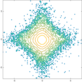
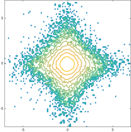
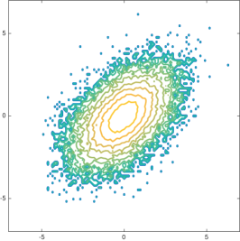
(a) Source

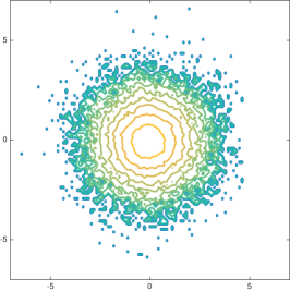
(b) ICA

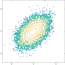
(c) Proposed Method

Figure 1: The logarithms of the non-parametric estimates of the two-dimensional probability density functions (a) for artificially generated source components, and (b,c) for estimated source components by ICA (maximum likelihood estimation without the decorrelation constraint as in (31)) and the proposed method, respectively. The first row is for independent non-Gaussian components, while the second one is for linearly correlated ones. The correlation coefficients in the second row are (a) 0.499, (b) 0.01 and (c) 0.472, respectively.

In this paper, we propose a novel method to estimate latent non-Gaussian components and their dependency structure simultaneously. The dependency structure includes both linear and higher-order correlations, and is parametrized by a single matrix. The off-diagonal elements of this dependency matrix represent the conditional dependencies much like the precision matrix does for Gaussian Markov random fields. More generally, the dependency matrix defines a distance matrix which can be used for visualization via an undirected graph, multidimensional scaling, or some other suitable technique. The proposed method can be interpreted as a generalization of ICA and correlated topographic analysis (CTA) (Sasaki ., 2013) where the dependency structures are assumed to be known. To develop the method, we begin with a new generative model for sources, which generalizes previous models of Hyvärinen . (2001); Karklin  Lewicki (2005); Osindero . (2006); Köster  Hyvärinen (2010) by capturing linear correlations between the components. The previous models generate non-Gaussian components without linear, but with higher-order correlations (Hyvärinen ., 2009, Section 9.3). Divisive normalization models (Heeger, 1992; Schwartz  Simoncelli, 2001; Ballé ., 2015) are also closely related, and focus on higher-order correlations.

Estimating two-layer models or Markov random fields for non-Gaussian components is often difficult because sophisticated parametric models generally have an intractable partition function so that the standard maximum likelihood estimation cannot be applied. To cope with this problem, several estimation methods have been proposed, such as contrastive divergence (Hinton, 2002), score matching (Hyvärinen, 2005), or noise contrastive estimation (Gutmann  Hyvärinen, 2012) and its extensions (Pihlaja ., 2010; Gutmann  Hirayama, 2011) (see Gutmann  Hyvärinen (20131) for an introductory paper). Score matching has a particularly useful property for the proposed model: The objective function for the estimation of the dependency parameters takes a simple quadratic form, and can be optimized by standard quadratic programming. Due to this computational simplification, here we use score matching, and empirically show that our method estimates the dependency structure and improves identifiability of the non-Gaussian components.

The paper is organized as follows: In Section 2, we begin with a novel probabilistic generative model for conditional precision matrices. Based on the generative model, we derive an approximation of the marginal density for non-Gaussian components where the dependency structure is explicitly parametrized like a precision matrix. Section 3 deals with estimation of the model, presenting a powerful algorithm for identifying the non-Gaussian components and their dependency structure. In Section 4, we perform numerical experiments and compare the proposed method with existing methods on artificial data. Section 5 demonstrates the applicability of the method to real data. Connections to past work and extensions of the proposed method are discussed in Section 6. Section 7 concludes this paper. A preliminary version of this paper was presented at AISTATS 2014 (Sasaki ., 2014).

2 Generative Model with Dependent Non-Gaussian Components

Here, we introduce a novel generative model with dependent non-Gaussian components. The probability density function (pdf) of the components and the data is shown to be only implicitly defined via an intractable integral. We derive an approximation of the pdf where the dependency structure of the components is explicitly parametrized, and demonstrate the validity of the approximation using both analytical arguments and simulations.

2.1 The Generative Model

As in previous work related to ICA (Hyvärinen  Oja, 2000), we assume a linear mixing model for the data,

$$\boldsymbol{x} =s_{1}\boldsymbol{a}_{1}+s_{2}\boldsymbol{a}_{2}+\dots+s_{d}\boldsymbol{a}_{d}=\mathbf{A}\boldsymbol{s},$$ (1)

where $\boldsymbol{x}=(x_{1},x_{2},\dots,x_{d})^{\top}$ denotes the $d$-dimensional data vector, $\mathbf{A}=(\boldsymbol{a}_{1},\boldsymbol{a}_{2},\dots,\boldsymbol{a}_{d})$ is the $d$ by $d$ mixing matrix formed by the basis vectors $\boldsymbol{a}_{i}$, and $\boldsymbol{s}=(s_{1},s_{2},\dots,s_{d})^{\top}$ is the $d$-dimensional vector consisting of the latent non-Gaussian components (the sources). The non-Gaussianity assumption about $\boldsymbol{s}$ is fundamental for the identification of the mixing model (Comon, 1994).

We next construct a model for the components $s_{i}$ which allows them to be statistically dependent, in contrast to ICA. We assume that $\boldsymbol{s}$ is generated from a Gaussian distribution with precision matrix $\mathbf{\Lambda}$ whose elements $\lambda_{ij}$ of $\mathbf{\Lambda}$ are random variables themselves, generated before $\boldsymbol{s}$ in a higher level of hierarchy as

$$\lambda_{ij}=\left\{\begin{array}[]{cc}-u_{ij},&i\neq j,\\ \sum_{k=1}^{d}u_{ik},&i=j.\end{array}\right.$$ (4)

The $u_{ij}$ are independent non-negative random variables, and because precision matrices are symmetric, we set $u_{ij}=u_{ji}$. To ensure invertability, we also require that $u_{ii}>0$. Nonzero $u_{ij}$ produce positive correlations between $s_{i}$ and $s_{j}$ (given the remaining variables), and larger values of $u_{ij}$ result in more strongly correlated variables. The motivation for the definition of the diagonal elements $\lambda_{ii}$ is that it guarantees realizations of $\mathbf{\Lambda}$ which are invertible and positive definite ($\mathbf{\Lambda}$ is symmetric and strictly diagonally dominant, from which the stated properties follow (see Theorem 6.1.10 in Horn  Johnson (1985) and Appendix E)). Readers familiar with graph theory will recognize that $\mathbf{\Lambda}$ equals the Laplacian matrix of a weighted graph defined by the matrix $\mathbf{U}$ with elements $u_{ij}$ (Bollobás, 1998).

Another property of the model is that the components $s_{i}$ are super-Gaussian: Hyvärinen . (2001) showed that the marginal pdfs of the Gaussian variables with random variances have heavier tails than a Gaussian pdf. Furthermore, since the conditional variances are dependent on each other in model (4), higher-order correlations are likely to exist (Hyvärinen ., 2001; Sasaki ., 2013).

We thus assume that the conditional pdf of $\boldsymbol{s}$ given $\mathbf{\Lambda}$ equals $p(\boldsymbol{s}|\mathbf{\Lambda})$,

$$p(\boldsymbol{s}|\mathbf{\Lambda}) =\frac{|\mathbf{\Lambda}|^{1/2}}{(2\pi)^{d/2}}\exp\left(-\frac{1}{2}\boldsymbol{s}^{\top}\mathbf{\Lambda}\boldsymbol{s}\right)$$ (5)

$$=\frac{|\mathbf{\Lambda}|^{1/2}}{(2\pi)^{d/2}}\exp\left(-\frac{1}{2}\sum_{i=1}^{d}\left\{\lambda_{ii}s_{i}^{2}+\sum_{j\neq i}\lambda_{ij}s_{i}s_{j}\right\}\right),$$ (6)

which we can write in terms of the $u_{ij}$ as $p(\boldsymbol{s}|\mathbf{U})$,

$$p(\boldsymbol{s}|\mathbf{U}) =\frac{|\mathbf{\Lambda}|^{1/2}}{(2\pi)^{d/2}}\exp\left(-\frac{1}{2}\sum_{i=1}^{d}\left\{s_{i}^{2}u_{ii}+\sum_{j>i}\left(s_{i}-s_{j}\right)^{2}u_{ij}\right\}\right),$$ (7)

as proved in Appendix A. While not explicitly visible from the notation, the determinant $|\mathbf{\Lambda}|$ is a function of the $u_{ij}$.

The specification of the distribution of the $u_{ij}$ completes the model, but this is a complex issue which we postpone to the next subsection. Denoting the pdf of the $u_{ij}$ generally by $p_{u}$, the pdf of the sources equals $p_{s}(\boldsymbol{s})$,

$$p_{s}(\boldsymbol{s})=\int_{0}^{\infty}p(\boldsymbol{s}|\mathbf{U})p_{u}(\mathbf{U})d\mathbf{U}.$$ (8)

and the pdf of $\boldsymbol{x}$ follows from the standard formula for linear transformations of random variables,

$$p_{x}(\boldsymbol{x})=p_{s}(\mathbf{W}\boldsymbol{x})|\mathbf{W}|,$$ (9)

with $\mathbf{W}=\mathbf{A}^{-1}$. However, since the determinant $|\mathbf{\Lambda}|$ in $p(\boldsymbol{s}|\mathbf{U})$ depends on $\mathbf{U}$, solving the multi-dimensional integral in (8) is practically impossible for any choice of $p_{u}$. While the integral can be estimated using Monte Carlo methods, it could be time-consuming. Therefore, we consider next an analytical approximation of the determinant which allows us to find an approximation of $p_{s}$ that holds qualitatively for any $p_{u}$. Once we have an approximation, $\tilde{p}_{s}$ say, we can use (9) to obtain a tractable approximation $\tilde{p}_{x}$ of the pdf of $\boldsymbol{x}$,

$$\tilde{p}_{x}(\boldsymbol{x})=\tilde{p}_{s}(\mathbf{W}\boldsymbol{x})|\mathbf{W}|.$$ (10)

2.2 Approximating the Density of the Dependent Non-Gaussian Components

In order to derive an approximation $\tilde{p}_{s}$ of $p_{s}$, we approximate the determinant of $\mathbf{\Lambda}$ via a product over the $u_{ii}$,

$$|\mathbf{\Lambda}| \approx\prod_{i=1}^{d}u_{ii}.$$ (11)

This is the only approximation which we need to obtain the tractable $\tilde{p}_{s}$ below. Another meaning of this approximation is to give a lower bound of $p(\boldsymbol{s}|\mathbf{U})$, and consequently $\tilde{p}_{s}$ is a lower-bound of $p_{s}$, which is proved by using the Ostrowski’s inequality in Appendix B. In other words, $\tilde{p}_{s}$ is an unnormalized model which is defined up to a multiplicative factor not depending on $\boldsymbol{s}$. This is not an insurmountable problem but needs to be taken into account when performing the estimation (see, for example, Gutmann  Hyvärinen, 20131).

Inserting the approximation (11) and the independence assumption of the $u_{ij}$ into (8) yields the following approximation of $p_{s}(\boldsymbol{s})$:

$$p_{s}(\boldsymbol{s})\approx \tilde{p}_{s}(\boldsymbol{s})$$

$$\propto \int_{0}^{\infty}\left[\prod_{i=1}^{d}\sqrt{u_{ii}}\right]\exp\left(-\frac{1}{2}\sum_{i=1}^{d}\left\{s_{i}^{2}u_{ii}+\sum_{j>i}\left(s_{i}-s_{j}\right)^{2}u_{ij}\right\}\right)p_{u}(\mathbf{U})d\mathbf{U}$$ (12)

$$\propto \int_{0}^{\infty}\left[\prod_{i=1}^{d}\sqrt{u_{ii}}\right]\left[\prod_{i=1}^{d}\exp\left(-\frac{1}{2}s_{i}^{2}u_{ii}\right)\prod_{j>i}\exp\left(-\frac{1}{2}(s_{i}-s_{j})^{2}u_{ij}\right)\right]\times$$

$$\left[\prod_{i=1}^{d}\prod_{j>i}p_{ij}(u_{ij})\right]d\mathbf{U},$$ (13)

where the product over the $p_{ij}$ in the last line is the pdf $p_{u}$ of the $u_{ij}$ due to their independence. The expression for $\tilde{p}_{s}$ can be simplified by grouping together terms featuring $u_{ii}$ and $u_{ij}$ only,

$$\tilde{p}_{s}(\boldsymbol{s})\propto \prod_{i=1}^{d}\left[\int_{0}^{\infty}\sqrt{u_{ii}}\exp\left(-\frac{1}{2}s_{i}^{2}u_{ii}\right)p_{ii}(u_{ii})du_{ii}\right]\times$$

$$\prod_{j>i}\left[\int_{0}^{\infty}\exp\left(-\frac{1}{2}\left(s_{i}-s_{j}\right)^{2}u_{ij}\right)p_{ij}(u_{ij})du_{ij}\right]$$ (14)

$$\propto \prod_{i=1}^{d}g_{ii}(s_{i}^{2})\prod_{j>i}g_{ij}((s_{i}-s_{j})^{2}),$$ (15)

where we have introduced the non-negative functions $g_{ii}(v)$ and $g_{ij}(v)$, defined for $v\geq 0$,

$$g_{ii}(v) \propto\int_{0}^{\infty}\sqrt{u_{ii}}\exp\left(-\frac{v}{2}u_{ii}\right)p_{ii}(u_{ii})du_{ii},$$ (16)

$$g_{ij}(v) \propto\int_{0}^{\infty}\exp\left(-\frac{v}{2}u_{ij}\right)p_{ij}(u_{ij})du_{ij}\;\text{ for }\;i\neq j.$$ (17)

The proportionality sign is used because $\tilde{p}_{s}$ is only defined up to the partition function. The approximation of the determinant thus allowed us to transform the multidimensional integral in (8) into a product of functions which are defined via one-dimensional integrals. The one-dimensional integrals can be easily solved numerically for arbitrary $p_{ij}$, or also analytically for particular choices of them. We also note that the $g_{ij}$ are related to the Laplace transform of the $p_{ij}$.

Different pdfs $p_{ij}$ yield different functions $g_{ij}$. But, Appendix C shows that unless $g_{ij}(v)$ is a constant, the different $\log g_{ij}(v)$ are monotonically decreasing convex functions for any choice of $p_{ij}$. We thus focus on the following particular class of functions

$$\log g_{ij}(v)=-m_{ij}\sqrt{v}+\mathrm{const}.$$ (18)

The $m_{ij}$ are free parameters which will be estimated from the data. They are symmetric, $m_{ij}=m_{ji}$. Further, we require that $m_{ii}>0$ so that $\tilde{p}_{s}$ depends on all $s_{i}$. For $m_{ij}$, $i\neq j$, we only require non-negativity: If $m_{ij}=0$, then $g_{ij}((s_{i}-s_{j})^{2})=\mathrm{const}$ which happens when the variable $u_{ij}$ is deterministically zero.

The particular choice (18) is motivated by its simplicity, but we show in Appendix D that it corresponds to choosing an inverse-Gamma distribution for the $u_{ij}$,

$$p_{ij}(u_{ij})=\left\{\begin{array}[]{cc}\frac{m_{ii}^{2}}{2}u_{ii}^{-2}\exp\left(-\frac{m^{2}_{ii}}{2u_{ii}}\right),&i=j,\\ \frac{m_{ij}}{\sqrt{2\pi}}u_{ij}^{-3/2}\exp\left(-\frac{m^{2}_{ij}}{2u_{ij}}\right),&i\neq j.\end{array}\right.$$ (19)

The parameters $m_{ij}$ determine the mode of the $p_{ij}$ (i.e. the point at which $p_{ij}$ is maximum): The mode is $m_{ii}^{2}/2$ for $i=j$ and $2m_{ij}^{2}/3$ otherwise.

Denoting by $\mathbf{M}$ the matrix formed by the $m_{ij}$, and its upper-triangular part by $\boldsymbol{m}$, $\boldsymbol{m}=(m_{11},\ldots m_{1d},m_{22},\ldots m_{2d},m_{33},\ldots,m_{3d},\ldots,m_{dd})$, we obtain the approximation $\tilde{p}_{s}(\boldsymbol{s})=\tilde{p}_{s}(\boldsymbol{s};\boldsymbol{m})$,

$$\tilde{p}_{s}(\boldsymbol{s};\boldsymbol{m})\propto\prod_{i=1}^{d}\exp\left(-m_{ii}|s_{i}|-\sum_{j>i}m_{ij}|s_{i}-s_{j}|\right),$$ (20)

which we will use in the following sections. The terms $|s_{i}|$ in (20) are related to modelling the $s_{i}$ as super-Gaussian, and the terms $|s_{i}-s_{j}|$ capture statistical dependencies between the components. The dependencies can be read out from the dependency matrix $\mathbf{M}$: If $m_{ij}=0$ for some $j\neq i$, $s_{i}$ is independent from the $s_{j}$ conditioned on the other variables. Furthermore, larger $m_{ij}$ imply stronger conditional (positive) dependencies between $s_{i}$ and $s_{j}$.

The model (20) generalizes pdfs used in previous work in the following ways:

1. $\tilde{p}$ approaches the Laplacian factorizable pdf when $m_{ij}\rightarrow 0$ for all $j\neq i$. Laplacian factorizable pdfs are often assumed for super-Gaussian components in ICA.

2. $\tilde{p}$ approaches the topographic pdf in CTA (Sasaki ., 2013) when $m_{ii}\rightarrow 1$, $m_{i,i+1}\rightarrow 1$ for all $i$ and $m_{ij}\rightarrow 0$ otherwise. The topographic pdf was derived using a different generative model and resorting to two quite heuristic approximations. This is contrast to this paper where a single relatively well-justified approximation was used. The new derivation is not only more elegant, but it allows for further extensions of the model as well, which is done in Appendix E.

3. $\tilde{p}$ was heuristically proposed in our preliminary conference paper (Sasaki ., 2014) as a simple extension of CTA. In this paper, on the other hand, we derived $\tilde{p}$ from a novel generative model for random precision matrices.

2.3 Numerical Validation of the Approximation

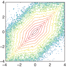
(a) Model

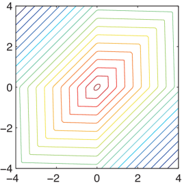
(b) Approximation

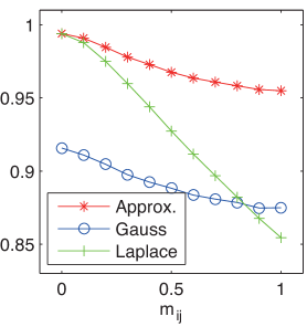
(c) Cosine

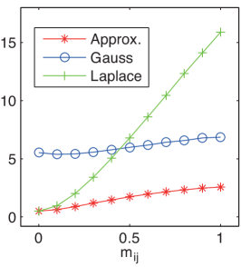
(d) KL divergence

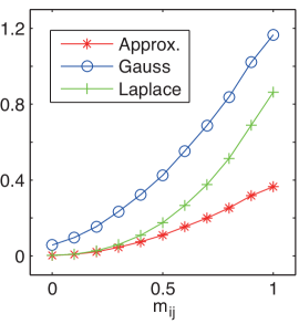
(e) Squared distance

Figure 2: Numerical validation of the approximation in (20). (a) Contour plots of a simple non-parametric estimate of the density $p_{s}$. (b) Contour plot of the approximation $\tilde{p}_{s}$. (c-e) Goodness of the approximation as a function of $m_{12}$. “Approx.” is the approximation; “Gauss” and “Laplace” are standard models (multivariate Gaussian density, and Laplace factorizable density, respectively). Note that for (c), larger is better, while for (d) and (e), smaller is better.

Here, we investigate the validity of the approximative pdf $\tilde{p}_{s}(\boldsymbol{s};\boldsymbol{m})$ in (20) using numerical simulations.

We generated a large number of samples for dependent non-Gaussian components according to the generative model in Section 2.1, fitted a nonparametric density to the sample, and compared it with our approximation in (20). The dimension of $\boldsymbol{s}$ was $d=2$ and the size of the sample was $T=10^{6}$. The $u_{ij}$ were drawn from the inverse-Gamma distribution in (19) with $m_{11}=m_{22}=1$. We performed the comparison for multiple $m_{12}$ between 0 and 1. Using the generated sample, the density $p_{s}$ in (8) was estimated as a normalized histogram. The approximative pdf $\tilde{p}_{s}(\boldsymbol{s},\boldsymbol{m})$ was normalized using numerical integration and evaluated with the same $m_{ij}$ used to generate the sample.

We evaluated the goodness of the approximation using three different measures,

$$\text{ang}(p_{s},\tilde{p}_{s}) =\frac{\sum_{l=1}^{N}\sum_{k=1}^{N}p_{s}(l,k)\tilde{p}_{s}(l,k)}{\sqrt{\sum_{l=1}^{N}\sum_{k=1}^{N}p_{s}(l,k)^{2}\sum_{l=1}^{N}\sum_{k=1}^{N}\tilde{p}_{s}(l,k)^{2}}},$$ (21)

$$\text{KL}(p_{s},\tilde{p}_{s}) =\sum_{l=1}^{N}\sum_{k=1}^{N}\log\frac{p_{s}(l,k)}{\tilde{p}_{s}(l,k)}p_{s}(l,k),$$ (22)

$$\text{SQ}(p_{s},\tilde{p}_{s}) =\sum_{l=1}^{N}\sum_{k=1}^{N}\left\{p_{s}(l,k)-\tilde{p}_{s}(l,k)\right\}^{2}p_{s}(l,k),$$ (23)

where $p_{s}(l,k)$ and $\tilde{p}_{s}(l,k)$ denote the values of the two-dimensional normalized histogram and the normalized $\tilde{p}_{s}(\boldsymbol{s};\boldsymbol{m})$ in bin $(l,k)$, respectively. Equation (21) is the cosine of the angle between $p_{s}$ and $\tilde{p}_{s}$, and the larger the value, the better the approximation. Equations (22) and (23) are the KL divergence and the expected squared distance, respectively. For comparison, we additionally computed these distance measures for a Laplace factorizable pdf with the same mean and marginal variance of the generated sources $\boldsymbol{s}$, and a Gaussian pdf with the same mean and covariance matrix.

The logarithms of $p_{s}$ and $\tilde{p}_{s}$ for $m_{12}=0.95$ are shown in Figure 2(a) and (b), respectively. The two pdfs seem to have similar properties in terms of the heavy-tailed profiles and linear correlations. Figures 2(c,d,e) show that $\tilde{p}_{s}$ approximates $p_{s}$ better than the Laplace and Gaussian distributions for all $m_{12}$. This is due to the fact that our approximation captures both the heavy-tails of $p_{s}$ and its dependency structure. Thus, we conclude that our approximation $\tilde{p}_{s}$ captures, at least qualitatively, the basic characteristics of the true distribution of the dependent non-Gaussian components.

3 Estimation of the Model

In this section, we first show how to estimate the linear mixing model (1) and the dependency matrix $\mathbf{M}$ formed by $\boldsymbol{m}$ using score matching, and then discuss important implementation details.

3.1 Using Score Matching for the Estimation

Approximating $p_{s}$ in (9) with $\tilde{p}_{s}$ from (20) yields an approximative pdf for the data as

$$p_{x}(\boldsymbol{x})\approx\tilde{p}_{x}(\boldsymbol{x};\mathbf{W},\boldsymbol{m})\propto\prod_{i=1}^{d}\exp\left(-m_{ii}|\boldsymbol{w}_{i}^{\top}\boldsymbol{x}|-\sum_{j>i}m_{ij}|\boldsymbol{w}_{i}^{\top}\boldsymbol{x}-\boldsymbol{w}_{j}^{\top}\boldsymbol{x}|\right)|\mathbf{W}|,$$ (24)

where $\boldsymbol{w}_{i}$ denotes the $i$-th row of $\mathbf{W}$. Both $\mathbf{W}$ and $\boldsymbol{m}$ are unknown parameters which we wish to estimate from a set of $T$ observations $\{\boldsymbol{x}_{1},\ldots,\boldsymbol{x}_{T}\}$ of $\boldsymbol{x}$. A conventional approach for the estimation would consist in maximizing the likelihood. However, maximum likelihood estimation cannot be done here because $\tilde{p}_{x}(\boldsymbol{x};\mathbf{W},\boldsymbol{m})$ is an unnormalized model, only defined up to a proportionality factor (partition function) which depends on $\boldsymbol{m}$. To cope with such estimation problems, several methods have been proposed (Hinton, 2002; Hyvärinen, 2005; Gutmann  Hyvärinen, 2012) (see Gutmann  Hyvärinen (20131) for a review paper). One of the methods is score matching (Hyvärinen, 2005) whose objective function for models from the exponential family is a quadratic form (Hyvärinen, 2007, Section 4). If $\mathbf{W}$ is fixed, $\tilde{p}_{x}$ in (24) belongs to the exponential family, so that estimation of $\boldsymbol{m}$ given an estimate of $\mathbf{W}$ would be straightforward with score matching. This motivated us to estimate the model in (24) by score matching, and to optimize its objective function by alternating between $\mathbf{W}$ and $\boldsymbol{m}$.

We next derive the score matching objective function $J(\mathbf{W},\boldsymbol{m})$ for the joint estimation of $\mathbf{W}$ and $\boldsymbol{m}$, and then show how it is simplified when $\mathbf{W}$ is considered fixed. By definition of score matching (Hyvärinen, 2005),

$$J(\mathbf{W},\boldsymbol{m}) =\frac{1}{T}\sum_{t=1}^{T}\sum_{k=1}^{d}\frac{1}{2}\psi_{k}(\boldsymbol{x}_{t};\mathbf{W},\boldsymbol{m})^{2}+\partial_{k}\psi_{k}(\boldsymbol{x}_{t};\mathbf{W},\boldsymbol{m}),$$ (25)

where $\psi_{k}$ and $\partial_{k}\psi_{k}$ are the first- and second-order derivatives of $\log\tilde{p}_{x}$ with respect to the $k$-th coordinate of $\boldsymbol{x}$,

$$\psi_{k}(\boldsymbol{x};\mathbf{W},\boldsymbol{m}) =\frac{\partial\log\tilde{p}_{x}(\boldsymbol{x};\mathbf{W},\boldsymbol{m})}{\partial x_{k}}, \partial_{k}\psi_{k}(\boldsymbol{x};\mathbf{W},\boldsymbol{m}) =\frac{\partial^{2}\log\tilde{p}(\boldsymbol{x};\mathbf{W},\boldsymbol{m})}{\partial x_{k}^{2}}.$$ (26)

For our model in (24), we have

$$\psi_{k}(\boldsymbol{x};\mathbf{W},\boldsymbol{m}) =-\sum_{i=1}^{d}m_{ii}G^{\prime}(\boldsymbol{w}_{i}^{\top}\boldsymbol{x})w_{ik}-\sum_{j>i}m_{ij}G^{\prime}(\boldsymbol{w}_{i}^{\top}\boldsymbol{x}-\boldsymbol{w}_{j}^{\top}\boldsymbol{x})(w_{ik}-w_{jk}),$$ (27)

$$\partial_{k}\psi_{k}(\boldsymbol{x};\mathbf{W},\boldsymbol{m}) =-\sum_{i=1}^{d}m_{ii}G^{\prime\prime}(\boldsymbol{w}_{i}^{\top}\boldsymbol{x})w_{ik}^{2}-\sum_{j>i}m_{ij}G^{\prime\prime}(\boldsymbol{w}_{i}^{\top}\boldsymbol{x}-\boldsymbol{w}_{j}^{\top}\boldsymbol{x})(w_{ik}-w_{jk})^{2},$$ (28)

where the absolute value in (20) is approximated by $|u|\approx G(u)=\log\cosh(u)$ for numerical stability, $G^{\prime}(u)=dG(u)/du=\tanh(u)$ and $G^{\prime\prime}(u)=\text{sech}^{2}(u)$.

Inspection of (27) and (28) shows that $\psi_{k}$ and $\partial\psi_{k}$ are linear functions of the $m_{ii}$ and $m_{ij}$. If we consider $\mathbf{W}$ fixed, and let $\boldsymbol{g}^{w}_{k}(\boldsymbol{x})$ be the column vector formed by the terms in (27) which are multiplied by the elements of $\boldsymbol{m}$, and let $\boldsymbol{h}^{w}_{k}(\boldsymbol{x})$ be the analogous vector for (28), we have $\psi_{k}(\boldsymbol{x};\mathbf{W},\boldsymbol{m})=\boldsymbol{m}^{\top}\boldsymbol{g}^{w}_{k}(\boldsymbol{x})$ and $\partial_{k}\psi_{k}(\boldsymbol{x};\mathbf{W},\boldsymbol{m})=\boldsymbol{m}^{\top}\boldsymbol{h}^{w}_{k}(\boldsymbol{x})$. The superscript “$w$” is used as a reminder that the vectors $\boldsymbol{g}_{k}^{w}(\boldsymbol{x})$ and $\boldsymbol{h}_{k}^{w}(\boldsymbol{x})$ depend on $\mathbf{W}$. For fixed $\mathbf{W}$, we can thus write $J(\mathbf{W},\boldsymbol{m})$ in (25) as a quadratic form $J(\boldsymbol{m}|\mathbf{W})$,

$$J(\boldsymbol{m}|\mathbf{W})=\frac{1}{2}\boldsymbol{m}^{\top}\left(\frac{1}{T}\sum_{t=1}^{T}\sum_{k=1}^{d}\boldsymbol{g}_{k}^{w}(\boldsymbol{x}_{t})\boldsymbol{g}_{k}^{w}(\boldsymbol{x}_{t})^{\top}\right)\boldsymbol{m}+\boldsymbol{m}^{\top}\left(\frac{1}{T}\sum_{t=1}^{T}\sum_{k=1}^{d}\boldsymbol{h}^{w}_{k}(\boldsymbol{x}_{t})\right).$$ (29)

For fixed $\mathbf{W}$, an estimate of $\boldsymbol{m}$ is obtained by minimizing $J(\boldsymbol{m}|\mathbf{W})$ under the constraint that the $m_{ii}$ are positive and the other $m_{ij}$ are nonnegative.

However, for estimation of $\mathbf{W}$, fixing $\boldsymbol{m}$ does not lead to an objective which takes a simpler form than $J(\mathbf{W},\boldsymbol{m})$ in (25). Therefore, we optimize $J(\mathbf{W},\boldsymbol{m})$ by a simple gradient descent whose details are given below.

3.2 Implementation Details

We estimate the parameters $\mathbf{W}$ and $\boldsymbol{m}$ of our statistical model (24) for dependent non-Gaussian components by alternately minimizing $J(\mathbf{W},\boldsymbol{m})$ in (25) with respect to $\mathbf{W}$ and $\boldsymbol{m}$. We next discuss some important details in this optimization scheme.

In our discussion of $\tilde{p}_{s}$ in (20), we noted that larger values of $m_{ij}$, $j>i$, indicate stronger (conditional) correlation between components $s_{i}$ and $s_{j}$. In preliminary simulations, we observed that, sometimes, the estimated $m_{ij}$ would take much larger values than the estimated $m_{ii}$, leading to estimated sources $\hat{s}_{i}$ and $\hat{s}_{j}$, and hence estimated features $\widehat{\boldsymbol{w}}_{i}$ and $\widehat{\boldsymbol{w}}_{j}$, which were almost the same. In order to avoid this kind of degeneracy, we imposed the additional constraint that a $m_{ii}$ had to be larger than the off-diagonal $m_{ij}$ summed together. Having this additional constraint, we found that the strict positivity constraint on the $m_{ii}$ could be relaxed to non-negativity. In summary, we imposed the following constraints on $\boldsymbol{m}$:

$$(\forall(i,j):i\leq j)\quad 0 \leq m_{ij}, (\forall i)\quad\sum_{j\neq i}m_{ij} \leq m_{ii}.$$ (30)

The constraints are linear, so that constrained minimization of $J(\boldsymbol{m}|\mathbf{W})$ can be done by standard methods from quadratic programming.

The mixing model (1) has a scale indeterminancy because dividing a feature by some number while multiplying the corresponding source by the same amount does not change the value of $\boldsymbol{x}$. While this scale indeterminancy is a well-known phenomenon in ICA, the situation is here more complicated because we have terms of the form $m_{ii}|\boldsymbol{w}_{i}^{\top}\boldsymbol{x}|$ and $m_{ij}|\boldsymbol{w}_{i}^{\top}\boldsymbol{x}-\boldsymbol{w}_{j}^{\top}\boldsymbol{x}|$ in the model-pdf instead of the more simple $|\boldsymbol{w}_{i}^{\top}\boldsymbol{x}|$ terms found in ICA. While in ICA, the scale indeterminancy is not a problem for maximum likelihood estimation, we have found that for our model, it was necessary to explicitly resolve the indeterminancy by imposing a unit norm constraint on the $\boldsymbol{w}_{i}$ (for whitened data).

For the optimization of $J(\mathbf{W},\boldsymbol{m})$, we have to choose some initial values for $\mathbf{W}$ and $\boldsymbol{m}$. We initialized $\mathbf{W}$ using a maximum-likelihood-based ICA algorithm, additionally imposing the norm constraint on the $\boldsymbol{w}_{i}$. In more detail, we initialized $\mathbf{W}$ as $\widehat{\mathbf{W}}$,

$$\widehat{\mathbf{W}} =\operatorname*{arg\,min}_{1\leq i\leq d,\|\boldsymbol{w}_{i}\|=1}J_{0}(\mathbf{W}), J_{0}(\mathbf{W}) =\frac{1}{T}\sum_{t=1}^{T}\sum_{i=1}^{d}G(\boldsymbol{w}_{i}^{\top}\boldsymbol{x}_{t})-\log|\det\mathbf{W}|.$$ (31)

Given the initial value $\widehat{\mathbf{W}}$, we obtained an initial value for $\boldsymbol{m}$ by minimizing $J(\boldsymbol{m}|\widehat{\mathbf{W}})$ in (29) under the constraints in (30).

While $J(\boldsymbol{m}|\mathbf{W})$ can be minimized by quadratic programming, minimization of $J_{0}(\mathbf{W})$ and $J(\mathbf{W},\boldsymbol{m})$ for fixed $\boldsymbol{m}$ has to be done by less powerful methods. We used a simple gradient descent algorithm where the step-size $\mu_{k}$ at each iteration $k$ was chosen adaptively by trying out $2\mu_{k-1}$ and $1/2\mu_{k-1}$ in addition to $\mu_{k-1}$, and selecting the one which yielded the smallest objective.

Algorithm 1 summarizes our approach to estimate the model (24), where it is assumed that the data have already been preprocessed by whitening and, optionally, dimension reduction by principal component analysis (PCA). In the proposed method, good initialization is important because the objective function has local optima, which can produce spurious correlations in the estimated $\boldsymbol{s}$. Therefore, we first perform ICA to give reasonable initialization both for $\mathbf{M}$ and $\mathbf{W}$. One weakness of the proposed method is that optimization for high-dimensional and large data can be slow compared with ICA because we alternately repeat Step 1 and 2. To alleviate this problem, in Section 5, we perform dimensionality reduction by PCA, and estimate $\mathbf{W}$ and $\mathbf{M}$ based on a randomly chosen subset of data samples at every repeat of Step 1 and 2.

 

Algorithm 1: Estimation of the mixing matrix $\mathbf{A}$ and dependency matrix $\mathbf{M}$

Input: Data $\{\boldsymbol{x}_{1},\boldsymbol{x}_{2},\dots,\boldsymbol{x}_{T}\}$ which have been whitened.

• Initialization (ICA): Compute $\widehat{\mathbf{W}}$ as in (31). Fixing $\mathbf{W}=\widehat{\mathbf{W}}$, compute $\widehat{\boldsymbol{m}}$ by minimizing $J(\boldsymbol{m}|\mathbf{W})$ in (29) under the constraints in (30), using a standard solver for quadratic programs.

• Repeat Step 1 and Step 2 until some conventional convergence criterion is met:

  1. Fixing $\boldsymbol{m}=\widehat{\boldsymbol{m}}$, update $\widehat{\mathbf{W}}$ by taking one gradient step to minimize $J(\mathbf{W},\boldsymbol{m})$ in (25) under the unit norm constraint on the rows $\boldsymbol{w}_{i}$ of $\mathbf{W}$.

  2. Fixing $\mathbf{W}=\widehat{\mathbf{W}}$, re-compute $\widehat{\boldsymbol{m}}$ by minimizing $J(\boldsymbol{m}|\mathbf{W})$ in (29) under the constraints in (30), using a standard solver for quadratic programs.

Output: Mixing matrix $\widehat{\mathbf{A}}=\widehat{\mathbf{W}}^{-1}$, dependency matrix $\widehat{\mathbf{M}}$ formed by $\widehat{\boldsymbol{m}}$.

 

4 Simulations on Artificial Data

In this section, using artificial data, we evaluate how well the proposed method identifies the sources and their dependency structure. The proposed method is compared to ICA and CTA.

4.1 Methods

For our evaluation, we used data generated according to the model in Section 2.1. We considered both data with independent components and data with components which had statistical dependencies within certain blocks. The interest of using independent components (sources) in the evaluation is to check that the model does not impose dependencies among the estimates when the underlying sources are truly independent. For the independent sources, the $u_{ii}$ in (4) were sampled from an inverse-Gamma distribution with shape parameter $k_{ii}=2$ and scale parameter $(m^{\prime}_{ii})^{2}=1$. The other elements $u_{ij},i\neq j$, were set to zero. Thus, $\mathbf{\Lambda}$ was a diagonal matrix, with $\lambda_{ii}=u_{ii}$, and the generated sources $s_{i}$ were statistically independent on each other. For the block-dependent sources, $\lambda_{ii}=\sum_{k=1}^{d}u_{ik}$ and $\lambda_{ij}=-u_{ij}$ as in (4). The $u_{ii}$ were for all $i$ from an inverse-Gamma distribution with shape parameter $k_{ii}=2$ and scale parameter $(m^{\prime}_{ii})^{2}=1$. The variables $u_{12}$, $u_{13}$ and $u_{23}$ were sampled from an inverse-Gamma distribution with shape parameter $k_{ii}=2$ and scale parameter $(m^{\prime}_{ij})^{2}=1/3$, while the remaining $u_{ij}$ were set to zero. With this setup, the $s_{1}$, $s_{2}$ and $s_{3}$ are statistically dependent while the other sources are conditionally independent. This dependency structure creates a block structure in the linear and energy correlation matrices where any pairs of $(s_{1},s_{2},s_{3})$ show relatively stronger dependencies than the other pairs (Figure 4 (c) and (d)). The energy correlation matrix is the correlation matrix of the squared random variables whose $(i,j)$-th element is given by

$$\frac{E\{s_{i}^{2}s_{j}^{2}\}-E\{s_{i}^{2}\}E\{s_{j}^{2}\}}{\sqrt{E\{(s_{i}^{2}-E\{s_{i}^{2}\})^{2}\}E\{(s_{j}^{2}-E\{s_{j}^{2}\})^{2}\}}},$$ (32)

where $E$ denotes the expectation and $E\{s_{i}\}=0$. After generating the sources, each component was standardized so that it has the zero mean and unit variance.

The observed data were generated from the mixing model (1) where the elements in $\mathbf{A}$ were sampled from the standard normal distribution. The data dimension was $d=10$ and the total number of observations was $T=20,000$. The preprocessing was whitening based on PCA. The performance matrix $\mathbf{P}=\mathbf{W}\mathbf{A}$ was used to visualize and evaluate the results. If $\mathbf{P}$ is close to a permutation matrix, the sources are well-identified.

To measure the goodness of the estimated dependency matrix, we used the scale parameters of the inverse-Gamma distributions employed to generate the sources in this simulation. For independent sources, first we constructed a reference matrix $\mathbf{M}^{\prime}$ by setting the diagonals and off-diagonals to $m_{ii}^{\prime}=1$ and zeros, respectively. To enable a comparison to the reference matrix, we normalize $\widehat{\mathbf{M}}$ by diving $\widehat{m}_{ij}$ by $\sqrt{\widehat{m}_{ii}\widehat{m}_{jj}}$ so that the diagonals are all ones, and denote the normalized $\widehat{\mathbf{M}}$ by $\widehat{\mathbf{M}}^{\prime}$. Finally, the goodness was measured by

$$\text{Error}_{\text{M}^{\prime}}=\|\mathbf{M}^{\prime}-\widehat{\mathbf{M}}^{\prime}\|_{\text{Fro}},$$ (33)

where $\|\cdot\|_{\text{Fro}}$ denotes the Frobenius norm. The reason of the error definition (33) is that since the different shape parameter $k_{ii}$ from the ones in the inverse-Gamma distribution (19) was used for numerical stability, we could not know the exact $\mathbf{M}$ and therefore had to focus on the relative values of the elements in $\widehat{\mathbf{M}}$. For block sources, we constructed the reference matrix by setting the diagonals in $\mathbf{M}^{\prime}$ to $1$, and the off-diagonals to $m_{ij}^{\prime}/\sqrt{\sum_{j=1}^{d}m_{ij}^{\prime}\sum_{i=1}^{d}m_{ji}^{\prime}}$ inside the block and to zeros outside the block. As a result, $\mathbf{M}^{\prime}$ becomes a diagonally dominant matrix with a block structure.

For comparison, we performed ICA and CTA (Sasaki ., 2013) on the same data. The ICA method was the same as the method used to initialize $\mathbf{W}$ in Algorithm 1, with the unit norm constraint on the rows $\boldsymbol{w}_{i}$ of $\mathbf{W}$. For all methods, to avoid local optima, we performed $10$ runs with different initialization of $\mathbf{W}$ and chose the run with the best value of each objective function. For ICA and CTA, after estimating $\mathbf{W}$, we estimated their dependency matrices by minimizing (29) with the same constraints (30).

4.2 Results

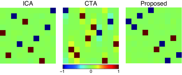
(a) Performance Matrices

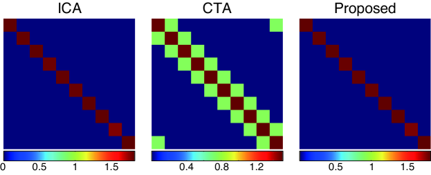
(b) Dependency Matrices

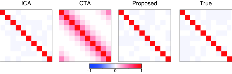
(c) Linear Correlation Matrices

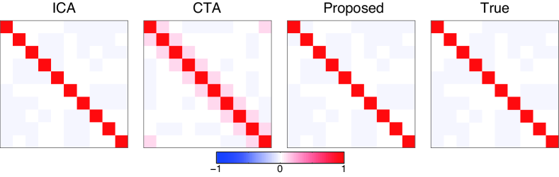
(d) Energy Correlation Matrices

Figure 3: Simulation results for independent sources. From (b) to (d), the permutation indeterminacy of ICA and the proposed method was compensated so that the largest element in each row of the performance matrix is on the diagonal. The true linear and energy correlation matrices of the sources are presented in the rightmost figures of (c) and (d).

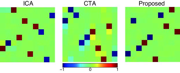
(a) Performance Matrices

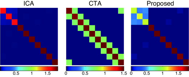
(b) Dependency Matrices

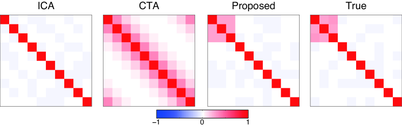
(c) Linear Correlation Matrices

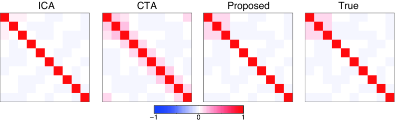
(d) Energy Correlation Matrices

Figure 4: Simulation results for block-dependent sources. From (b) to (d), the permutation indeterminacy of ICA and the proposed method was compensated so that the largest element in each row of the performance matrix is on the diagonal.

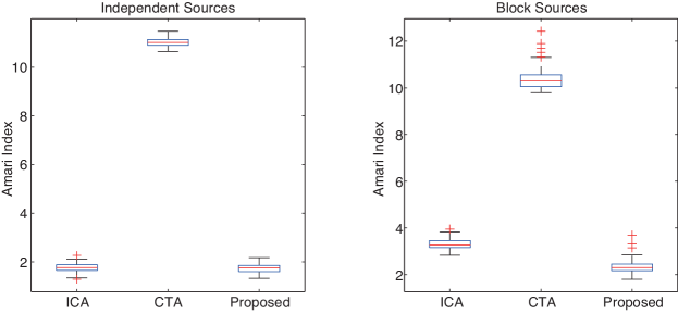
(a) Amari Index

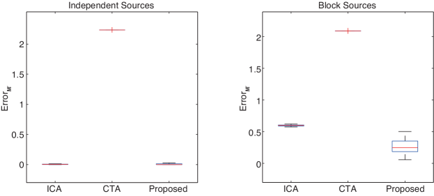
(b) $\text{Error}_{\text{M}^{\prime}}$

Figure 5: Estimation error for $100$ runs, for both independent and block sources, summarized in terms of Amari index and Error${}_{\text{M}^{\prime}}$. In the comparisons, ICA and CTA were used to estimate $\mathbf{W}$, and their dependency matrices were estimated by minimizing the objective in (29) with the same constraints (30).

We first report the performance on a single dataset, and then the average performance on $100$ randomly generated datasets. The results for the independent sources from the single dataset are presented in Figure 3. For ICA and the proposed method, the performance matrices are close to permutation matrices (Figure 3(a)), the estimated dependency matrices resemble a diagonal matrix (Figure 3(b)), as they should be, and the correlation matrices are almost diagonal (Figures 3(c) and (d)). For CTA, on the other hand, the performance matrix includes more cross-talk, the dependency matrix is tri-diagonal, and the linear and energy correlation matrices are clearly different from a diagonal matrix. These unsatisfactory results for CTA come from the fact that the dependency structure of CTA is pre-fixed, and thus CTA forcibly imposes linear correlations among the estimated neighboring components even though the original components are linearly uncorrelated. This drawback has been already reported by Sasaki . (2013). In contrast, the proposed method learned automatically that the sources are independent, and solved the identifiability issue of CTA.

The results for block-dependent sources are shown in Figure 4. The proposed method separates the sources, that is, estimates the linear components, with good accuracy, while ICA has more errors. The performance matrix for CTA includes again a lot of cross-talk (Figure 4(a)). Regarding $\mathbf{M}$ and the correlations matrices, we compensated for the permutation indeterminacy of the sources for both ICA and the proposed method so that the largest element in each row of the performance matrix is on the diagonal. Figure 4(b) shows that the proposed method yields a dependency matrix with a clearly visible block structure in the upper left corner, while ICA and CTA do not. In addition, the linear and energy correlation matrices have the block structure for the proposed method, while ICA and CTA do not produce it (Figure 4(c) and (d)). Thus, only the proposed method was able to correctly identify the dependency structure of the latent sources.

We further analyzed the average performance for $100$ randomly generated datasets. Figure 5(a) shows the distribution of the Amari index (AI) (Amari ., 1996) for the independent and block-dependent sources. AI is an established measure to assess the performance of blind source separation algorithms, and a smaller value means better performance. For independent sources, the proposed method has almost the same performance as ICA, while the performance of CTA is much worse. For block-dependent sources, the performance of the proposed method is better than ICA and CTA. This result means that when the original sources $s_{i}$ are linearly correlated, ICA is not the best method in terms of identifiability of the mixing matrix, and that taking into account the dependency structure for linear correlations improves the identifiability.

For the goodness of the estimated dependency matrix, we plot the distribution of Error${}_{\mathbf{M}^{\prime}}$ in Figure 5(b). In this analysis, the permutation indeterminacy was compensated as done in Figure 4. The plot confirms the qualitative findings in Figures 3 and 4: the proposed method is able to capture the dependency structure of the sources better than ICA and CTA.

5 Application to Real Data

This section demonstrates the applicability of the proposed method on two kinds of real data: speech data and natural image data.

Basic ICA and related methods based on energy (square) correlation work well on raw speech and image data, due to the symmetry of the data distributions. The symmetry implies in particular that positive and negative values of linear features are to some extent equivalent, as implicitly assumed in computation of Fourier spectra or complex cell outputs in models of early (mammalian) vision, which is compatible with energy correlations.

However, on higher levels of feature extraction, such symmetry cannot be found anymore, and energy correlations cannot be expected to be meaningful. Our goal here is to apply our new method on such higher-level features, where linear correlations are likely to be important. In particular, we use speech spectrograms, and outputs of complex cells simulating computations in the visual cortex, respectively.

5.1 Speech Data

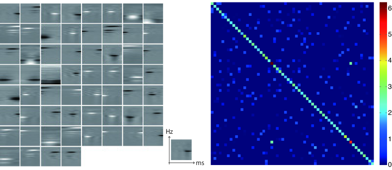
(a) Estimated basis vectors (left) and dependency matrix (right)

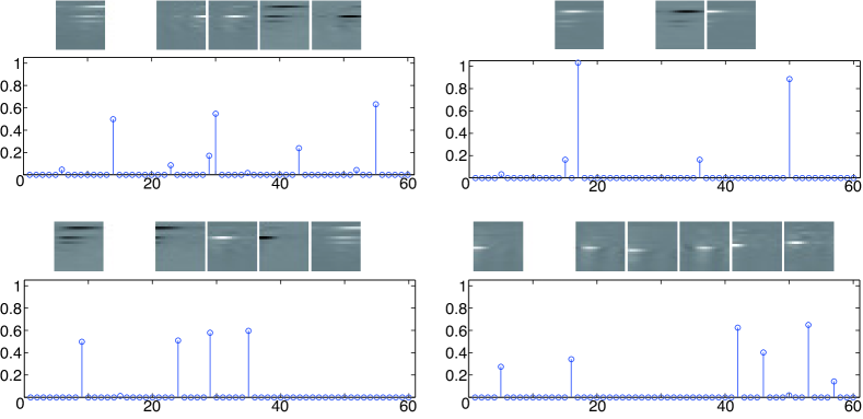
(b) For a selected $i$, the $m_{ij}$ as stem plots, and the corresponding basis vectors with strong $m_{ij}$ (the left-most being $\widehat{\boldsymbol{a}}_{i}$ and the others $\widehat{\boldsymbol{a}}_{j}$)

Figure 6: Results for speech (spectrogram) data.

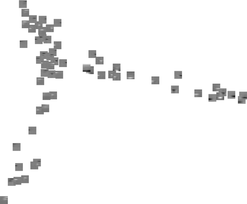
Figure 7: Speech data: Visualization of the estimated dependency structure between features (basis vectors) by MDS. In the figure, features with stronger $m_{ij}$ should be closer to each other in this visualization. The positions of some too close or too far-away features were magnified in order to show all features in a reasonable scale.

Previously, sparse coding (Olshausen  Field, 1996) and ICA-related-methods have been applied to audio data to investigate the basic properties of cells in the primary auditory cortex (A1) (Klein ., 2003; Terashima  Hosoya, 2009; Terashima ., 2013). More recently, topographic ICA (TICA) (Hyvärinen ., 2001) was employed to analyze spectrogram data, and feature maps were learned which are similar to the tonotopic maps in A1 (Terashima  Okada, 2012). However, in TICA, the dependency structure is influenced by higher-order correlations only and it is fixed to nearby components beforehand. Furthermore, using energy correlations for spectrograms may not be well justified. Here, we lift these restrictions and learn the dependency structure from the data by taking both linear and higher-order correlations between the latent sources into account.

Following Terashima  Okada (2012), we used human narratives data (International Phonetic Association, 1999). The data were down-sampled to $8$ kHz, and the spectrograms were computed by using the NSL toolbox. After re-sizing the vertical (spectral) size of the spectrograms from $128$ to $20$, short spectrograms were randomly extracted with the horizontal (temporal) size equal to $20$. The vectorized spectrogram patches were our $T=100,000$ input data points $\{\boldsymbol{x}_{1},\boldsymbol{x}_{2},\dots,\boldsymbol{x}_{T}\}$.

As preprocessing, we removed the DC component of each $\boldsymbol{x}_{t}$, and then rescaled each $\boldsymbol{x}_{t}$ to unit norm. Finally, whitening and dimensionality reduction were performed simultaneously by PCA. We retained $d=60$ dimensions. To reduce the computational cost, in this experiment, at every repeat of Step 1 and 2 in Algorithm 1, we randomly selected $30,000$ data points from $T=100,000$ data points to be used for estimation.

The estimated basis vectors $\boldsymbol{a}_{i}$ will be visualized in the original domain as spectrograms. For the estimated dependency matrix, we apply a multidimensional scaling (MDS) method to $\widehat{\mathbf{M}}$ to visualize the dependency structure on the two-dimensional plane. To employ MDS, we constructed a distance matrix from $\widehat{\mathbf{M}}$ similarly as done in Hurri  Hyvärinen (2003): We first normalized each element $\widehat{\boldsymbol{m}}_{ij}$ by $\sqrt{\widehat{\boldsymbol{m}}_{ii}\widehat{\boldsymbol{m}}_{jj}}$ to make the diagonals ones, then computed the square root of each element in the normalized matrix, and finally subtracted each element from one. The purpose of MDS is to project the points in a high-dimensional space to the two-dimensional plane so that the distance in the high-dimensional space is preserved as much as possible in the two-dimensional space. Thus, applying MDS should yield a representation where the dependent features (basis vectors) are close to each other.

The estimated basis vectors $\hat{\boldsymbol{a}}_{i}$ and dependency matrix $\widehat{\mathbf{M}}$ are presented in Figure 6(a). Most of the basis vectors show vertically (spectrally) and horizontally (temporally) localized patterns with single or multiple peaks. These properties have been also found in previous work (Terashima  Okada, 2012). But, unlike previous work, we also estimated the dependency structure from the data. As shown in the right panel of Figure 6(a), the off-diagonal elements of the dependency matrix are sparse: most of the elements are zero. Figure 6(b) shows that basis vectors with similar peak frequencies tend to have strong (conditional) dependencies. The visualization of $\widehat{\mathbf{M}}$ further globally supports this observation (Figure 7).

Compared with previous work, the properties of nearby features in Figure 7 seem to be more consistent: Nearby features tend to have similar peak positions along with the spectral (vertical) axis, while the peak positions on the temporal (horizontal) axis are more random. On the other hand, Terashima  Okada (2012) found that nearby features often show different peak positions on the spectral axis, and the estimated features on the topographic map are locally disordered. These results may reflect that linear correlations in sound spectrogram data should be important dependencies, and that the proposed method captured the structure in the data better than TICA.

5.2 Outputs of Complex Cells

We next apply our method to the outputs of simulated complex cells in the primary visual cortex when stimulated with natural image data. Previously, ICA, non-negative sparse coding and CTA have been applied to this kind of data, and some prominent features such as long contours and topographic maps have been learned (Hoyer  Hyvärinen, 2002; Hyvärinen ., 2005; Sasaki ., 2013). However, these methods have either assumed that the features are independent, or pre-fixed their dependency structure. Our method removes this restriction and learns the dependency structure from the data.

As in the previous work cited above, we computed the outputs of the simulated complex cells $\boldsymbol{x}$ as

$$x^{\prime}_{k} =\left(\sum_{x,y}W_{k}^{o}(x,y)I(x,y)\right)^{2}+\left(\sum_{x,y}W_{k}^{e}(x,y)I(x,y)\right)^{2},$$

$$x_{k} =\log(x^{\prime}_{k}+1.0),$$

where $I(x,y)$ is a $24\times 24$ natural image patch, and $W_{k}^{o}(x,y)$ and $W_{k}^{e}(x,y)$ are odd- and even-symmetric Gabor functions with the same spatial positions, orientation and frequency. The total number of outputs was $T=100,000$. The complex cells were arranged on a $6$ by $6$ spatial grid, having $4$ orientations each. In total, there were $144$ cells. Since the simulated complex cells in this experiment are stimulated by natural images, we regard this data as real data. We performed the same preprocessing steps as in Section 5.1 above; the dimensionality was here reduced to $d=60$. As in the last section, to reduce the computational cost, we randomly selected a subset of data points from the whole data points at every repeat of the two steps in Algorithm 1. We visualized the basis vectors as in previous work (Hoyer  Hyvärinen, 2002; Hyvärinen ., 2005): Each basis vector is visualized by ellipses which have the orientation and spatial position preferences of the underlying complex cells.

The estimated basis vectors $\hat{\boldsymbol{a}}_{i}$ and the dependency matrix $\widehat{\mathbf{M}}$ are presented in Figure 8. One prominent kind of features among the basis vectors are long contours, as also found in previous work (Hoyer  Hyvärinen, 2002; Hyvärinen ., 2005).

Unlike in previous work, we also learned the dependencies between the features. As with the speech data, the off-diagonal elements of the dependency matrix are sparse (Figure 8(a), right), and similar features tend to have stronger dependencies (Figure 8(b)).

Figure 9 visualizes the dependency structure by MDS as in Section 5.1. This visualization supports the observation that the contour features tend to have stronger dependencies. In particular, it is often the case that contour-features are closer to other contour-features which are slightly shifted along their non-preferred orientation. If put together, such two contour-features would form either a broader contour of the same orientation or a slightly bent even longer contour. This property is in line with higher-level features learned using a three-layer model of natural images (Gutmann  Hyvärinen, 20132).

We further investigate whether the proposed method estimated linearly correlated components on real data in contrast to previous energy-correlation-based methods (Karklin  Lewicki, 2005; Osindero ., 2006; Köster  Hyvärinen, 2010). Figure 10 shows a scatter plot for linear and energy correlation coefficients for all the pairs of estimated components. As the sparsity of $\widehat{\mathbf{M}}$ implies, most pairs have only weak statistical dependencies. However, some pairs show both strong linear and energy correlations. Thus, the proposed method did find linearly correlated components on real data as well.

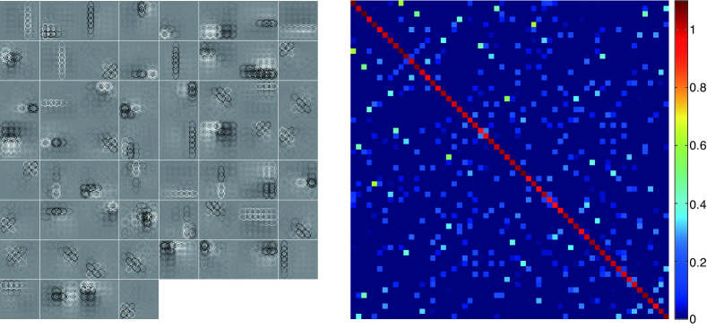
(a) Estimated basis vectors (left) and dependency matrix (right)

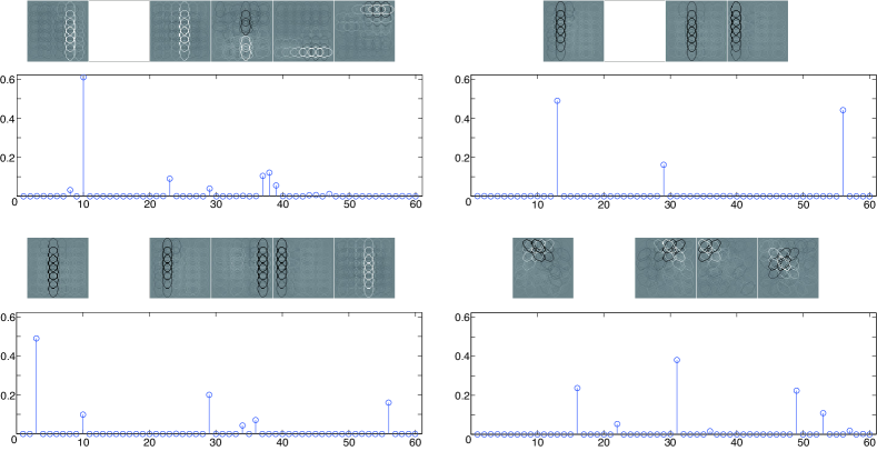
(b) For a selected $i$, the $m_{ij}$ as stem plots, and the corresponding basis vectors with stronger $m_{ij}$ (the left-most being $\widehat{\boldsymbol{a}}_{i}$ and the others $\widehat{\boldsymbol{a}}_{j}$)

Figure 8: Results for the simulated complex cell data.

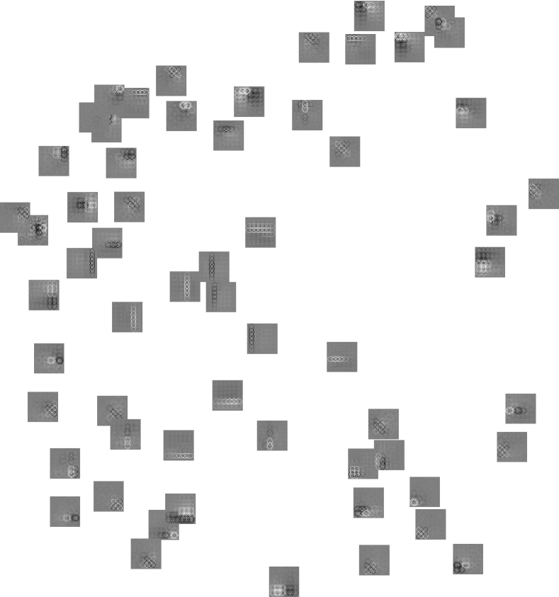
Figure 9: Complex cell outputs: Visualization of the estimated dependency structure between features (basis vectors) by MDS. In the graph, features with stronger $m_{ij}$ should be closer to each other in this visualization.

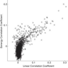
Figure 10: A scatter plot for linear and energy correlation coefficients from the estimated sources. Each point corresponds to one pair of estimated components $(\widehat{s}_{i},\widehat{s}_{j})$.

6 Discussion

We discuss some connections to previous work and possible extensions of the proposed method.

6.1 Connection to Previous Work

We proposed a novel method to simultaneously estimate non-Gaussian components and their dependency (correlation) structure. So far, a number of methods to estimate non-Gaussian components have been proposed: ICA assumes that the latent non-Gaussian components are statistically independent, and ISA (Hyvärinen  Hoyer, 2000) and topographic methods (Hyvärinen ., 2001; Mairal ., 2011; Sasaki ., 2013) pre-fix the dependency structure inside pre-defined groups of components, or overlapping neighborhoods of components. Methods to estimate tree-dependency structures have also been proposed (Bach  Jordan, 2003; Zoran  Weiss, 2009). In contrast to these methods, our method does not make any assumptions on the dependency structure to be estimated.

Some methods based on two-layer models also estimate the dependency structures of non-Gaussian components from data (Karklin  Lewicki, 2005; Osindero ., 2006; Köster  Hyvärinen, 2010). Most of the methods mainly focus on high-order correlations, assuming that the components are linearly uncorrelated. The method proposed by Osindero . (2006) can estimate an overcomplete model as well, which necessarily makes the estimated components linearly correlated; however, it is unclear in what way such linear correlations reflect the dependency structure of the underlying sources. Our method models both linear and higher-order correlations explicitly. As a new theoretical approach, in this paper, we proposed a generative model for random precision matrices. The proposed generative model generalizes a previous generative model for sources used in existing two-layer methods (Karklin  Lewicki, 2005; Osindero ., 2006): The previous model corresponds to a special case in our model where the off-diagonal elements are deterministically zero.

Another line of related work is graphical models for latent factors (He ., 2012). This work assumes that both the latent factors and the undirected graph are sparse. The main goal of that approach is to estimate a latent lower-dimensional representation of the input data where pair-wise dependencies between latent factors are represented by an undirected graph. The main difference to our work is that He . (2012) use a constant precision matrix instead of a stochastic one, and thus that they do not really model non-Gaussian components. Instead, He . (2012) emphasize sparsity in the sense that the undirected graphs to be estimated have sparse edges. As discussed below, our method can be easily extended to include the sparsity constraint while still keeping the objective function a simple quadratic form.

6.2 Extensions of the Proposed Method

Next, we discuss some extensions of our model which could be considered in future work. One extension of the proposed method would be to incorporate prior information or an additional constraint on $\mathbf{M}$. Recently, a number of methods to estimate sparse Gaussian graphical models has been proposed (Friedman ., 2008; Banerjee ., 2008). In our method, the sparseness constraint on $m_{ij}$ can be easily incorporated into the objective function $J(\boldsymbol{m}|\mathbf{W})$ in (29) yielding $J_{\lambda}(\boldsymbol{m}|\mathbf{W})$,

$$J_{\lambda}(\boldsymbol{m}|\mathbf{W}) =J(\boldsymbol{m}|\mathbf{W})+\lambda\boldsymbol{m}^{\top}\boldsymbol{1},$$ (34)

where $\lambda$ is the regularization parameter, and $\boldsymbol{1}$ is a vector of ones. The objective function $J_{\lambda}(\boldsymbol{m}|\mathbf{W})$ is still a quadratic form and its minimization is not more difficult than the minimization of $J(\boldsymbol{m}|\mathbf{W})$. However, this extension involves selecting the parameter $\lambda$, which adds a complexity to the problem which need to be solved. In practice, we may perform cross-validation (CV) under some criterion, but employing CV is computationally demanding especially in our alternate optimization. Therefore, selecting an appropriate value of $\lambda$ is an issue in the future.

Another extension would be to estimate additional parameters modelling linear correlations. As shown in Appendix E, the model for the sources in (20) can be generalized to

$$\tilde{p}_{s}(\boldsymbol{s};\boldsymbol{m},\mathbf{\Theta}) \propto\prod_{i=1}^{d}\exp\left(-\theta_{ii}m_{ii}|s_{i}|-\sum_{j>i}m_{ij}\sqrt{\theta_{ii}s_{i}^{2}+\theta_{jj}s_{j}^{2}+2\theta_{ij}s_{i}s_{j}}\right),$$

where the $\theta_{ii}$ are positive parameters and $\theta_{ij}\in\left\{-1,0,1\right\}$ for $i\neq j$. The pdf in (20) is a special case of the above pdf: it is obtained for $\theta_{ii}=1$ and $\theta_{ij}=-1$ for $i\neq j$. Thus, by estimating all the $\theta_{ij}$, we can estimate more complex dependency structures, generalizing our method. However, estimating $\theta_{ij}$ leads a complicated optimization problem because the objective function for score matching is no longer a quadratic form, and the $\theta_{ij}$ are discrete variables. That is why we decided to use the simpler model in (20) and leave this interesting challenge for future work.

7 Conclusion

In this paper, we proposed a method to simultaneously estimate non-Gaussian components and their dependency structure. The dependency structure is defined in terms of both linear and higher-order correlations, can be represented in a convenient form, and thus can be readily interpreted. Using score matching, the estimation of the dependency structure is particularly simple because the objective function takes a quadratic form and can be minimized using standard methods from quadratic programming.

The proposed method generalizes previous methods: Independent component and correlated topographic analysis both assume pre-fixed dependency structures for the non-Gaussian components, while our method flexibly estimates the dependency structure from the data themselves. Several existing methods based on two-layer models also aim at estimating the dependency structure, but they focus on higher-order correlations, ignoring linear correlations.

We experimentally demonstrated on artificial data that the proposed method improves identifiability of latent non-Gaussian components over existing methods by learning their dependency structure, and application to the outputs of simulated complex cells and the spectrograms of natural audio data unveiled new kinds of relationships among the latent non-Gaussian components.

Acknowledgments

H. Sasaki carried out most of the work when he was a JSPS fellow at the University of Electro-Communications. The work was partly done when M. U. Gutmann was with the Department of Mathematics and Statistics, University of Helsinki, and supported by the Finnish Centre of Excellence in Computational Inference Research COIN. H. Shouno was partly supported by MEXT/KAKENHI JSPS KAKENHI Grant 26120515. A. Hyvärinen was supported by the Academy of Finland (Centre of Excellence in Inverse problems).

Appendix

Appendix A Calculations for (7)

With (4), the conditional pdf (6) can be written as

$$p(\boldsymbol{s}|\mathbf{U}) =\frac{|\mathbf{\Lambda}|^{1/2}}{(2\pi)^{d/2}}\exp\left(-\frac{1}{2}\sum_{i=1}^{d}\left\{\lambda_{ii}s_{i}^{2}+\sum_{j\neq i}\lambda_{ij}s_{i}s_{j}\right\}\right),$$ (35)

$$=\frac{|\mathbf{\Lambda}|^{1/2}}{(2\pi)^{d/2}}\exp\left(-\frac{1}{2}\sum_{i=1}^{d}\left\{s_{i}^{2}\sum_{k=1}^{d}u_{ik}-\sum_{j\neq i}s_{i}s_{j}u_{ij}\right\}\right),$$ (36)

$$=\frac{|\mathbf{\Lambda}|^{1/2}}{(2\pi)^{d/2}}\exp\left(-\frac{1}{2}\sum_{i=1}^{d}\left\{s_{i}^{2}u_{ii}+\sum_{k\neq i}s_{i}^{2}u_{ik}-\sum_{j\neq i}s_{i}s_{j}u_{ij}\right\}\right).$$ (37)

Since the $u_{ij}$ are symmetric, we have further

$$p(\boldsymbol{s}|\mathbf{U}) =\frac{|\mathbf{\Lambda}|^{1/2}}{(2\pi)^{d/2}}\exp\left(-\frac{1}{2}\sum_{i=1}^{d}\left\{s_{i}^{2}u_{ii}+\sum_{k>i}\left(s_{i}^{2}+s_{k}^{2}\right)u_{ik}-2\sum_{j>i}s_{i}s_{j}u_{ij}\right\}\right),$$ (38)

$$=\frac{|\mathbf{\Lambda}|^{1/2}}{(2\pi)^{d/2}}\exp\left(-\frac{1}{2}\sum_{i=1}^{d}\left\{s_{i}^{2}u_{ii}+\sum_{j>i}\left(s_{i}-s_{j}\right)^{2}u_{ij}\right\}\right),$$ (39)

which is (7).

Appendix B Approximation of the Determinant in (11)

We prove that (11) approximates the determinant with a lower bound and that the resulting approximation $\tilde{p}_{s}$ of the source density $p_{s}$ is an unnormalized model.

By definition in (4), $\mathbf{\Lambda}$ is a strictly diagonally dominant matrix. Ostrowski’s inequality (Ostrowski, 1937) thus yields

$$|\mathbf{\Lambda}| \geq\prod_{i=1}^{d}\left(\lambda_{ii}-\sum_{\begin{subarray}{c}j=1\\ j\neq i\end{subarray}}^{d}\lambda_{ij}\right),$$ (40)

and by definition of the $\lambda_{ij}$ in (4), we obtain

$$|\mathbf{\Lambda}| \geq\prod_{i=1}^{d}\left(\sum_{j=1}^{d}u_{ij}-\sum_{\begin{subarray}{c}j=1\\ j\neq i\end{subarray}}^{d}u_{ij}\right)=\prod_{i=1}^{d}u_{ii},$$ (41)

which shows that the approximation (11) corresponds to a lower bound of the determinant.

Applying the approximation of the determinant to $p(\boldsymbol{s}|\mathbf{U})$ in (7) gives $\tilde{p}(\boldsymbol{s}|\mathbf{U})$,

$$\tilde{p}(\boldsymbol{s}|\mathbf{U}) =\frac{\prod_{i=1}^{d}\sqrt{u_{ii}}}{(2\pi)^{d/2}}\exp\left(-\frac{1}{2}\sum_{i=1}^{d}\left\{s_{i}^{2}u_{ii}+\sum_{j>i}\left(s_{i}-s_{j}\right)^{2}u_{ij}\right\}\right),$$ (42)

which is a lower bound for $p(\boldsymbol{s}|\mathbf{U})$ due to (41),

$$\tilde{p}(\boldsymbol{s}|\mathbf{U})\leq p(\boldsymbol{s}|\mathbf{U}).$$ (43)

Using the approximation $\tilde{p}(\boldsymbol{s}|\mathbf{U})$ instead of $p(\boldsymbol{s}|\mathbf{U})$ in (8) yields an approximation $\tilde{p}_{s}$ of the pdf of the dependent non-Gaussian components which inherits the lower bound property,

$$\tilde{p}_{s}(\boldsymbol{s})=\int_{0}^{\infty}\tilde{p}(\boldsymbol{s}|\mathbf{U})p_{u}(\mathbf{U})d\mathbf{U}\leq\int_{0}^{\infty}p(\boldsymbol{s}|\mathbf{U})p_{u}(\mathbf{U})d\mathbf{U}=p_{s}(\boldsymbol{s}).$$ (44)

Since $p_{s}$ integrates to one, we have

$$\int\tilde{p}_{s}(\boldsymbol{s})d\boldsymbol{s}\leq 1,$$ (45)

which means that $\tilde{p}_{s}$ is an unnormalized model.

Appendix C Properties of the Nonlinearities in (17)

We here investigate properties of the nonlinearities $g_{ij}(v)$ in (17). It is shown that, unless constant, the $\log g_{ij}(v)$ are monotonically decreasing convex functions.

For the analysis, it is helpful to introduce the functions $\phi_{ij}(u)$, $u\geq 0$,

$$\phi_{ij}(u)=\begin{cases}\sqrt{u}p_{ii}(u)&\mbox{if }i=j\\ p_{ij}(u)&\mbox{otherwise},\end{cases}$$ (46)

which allow us to rewrite the $g_{ij}(v)$ as

$$g_{ij}(v)=\int_{0}^{\infty}\exp\left(-\frac{1}{2}vu\right)\phi_{ij}(u)du,\quad v\geq 0,$$ (47)

for all $(i,j)$. The functions $\phi_{ij}$ are non-negative but they are not pdfs if $i=j$ because they do not integrate to one. We note that $g_{ij}$, $i\neq j$, is constant if $p_{ij}$ corresponds to a Dirac measure concentrated at zero, that is, to a $u_{ij}$ which is deterministically zero. In what follows, we assume that the $p_{ij}$ are pdfs with nonzero variance.

The derivative of $\log g_{ij}(v)$ is

$$\frac{\partial\log g_{ij}(v)}{\partial v} = \frac{\frac{\partial g_{ij}(v)}{\partial v}}{g_{ij}(v)}$$ (48)

$$= \frac{-\frac{1}{2}\int_{0}^{\infty}u\exp\left(-\frac{1}{2}vu\right)\phi_{ij}(u)du}{\int_{0}^{\infty}\exp\left(-\frac{1}{2}vu\right)\phi_{ij}(u)du},$$ (49)

which is negative for all $v>0$. Importantly, the derivative is related to the expected value $\mu_{ijv}$ of the pdf $\gamma_{ijv}(u)$,

$$\gamma_{ijv}(u)=\frac{\exp\left(-\frac{1}{2}vu\right)\phi_{ij}(u)}{\int_{0}^{\infty}\exp\left(-\frac{1}{2}vu\right)\phi_{ij}(u)du},$$ (50)

that is,

$$\frac{\partial\log g_{ij}(v)}{\partial v}=-\frac{1}{2}\mu_{ijv}.$$ (51)

The second derivative equals

$$\frac{\partial^{2}\log g_{ij}(v)}{\partial v^{2}} = \frac{\partial^{2}g_{ij}(v)}{\partial v^{2}}\frac{1}{g_{ij}(v)}-\left(\frac{\partial g_{ij}(v)}{\partial v}\right)^{2}\frac{1}{g_{ij}(v)^{2}}$$ (52)

$$= \frac{\partial^{2}g_{ij}(v)}{\partial v^{2}}\frac{1}{g_{ij}(v)}-\left(\frac{\partial\log g_{ij}(v)}{\partial v}\right)^{2}$$ (53)

$$= \frac{\partial^{2}g_{ij}(v)}{\partial v^{2}}\frac{1}{g_{ij}(v)}-\frac{1}{4}\mu_{ijv}^{2},$$ (54)

which can be written in terms of the variance of the pdf $\gamma_{ijv}$: We have

$$\frac{\partial^{2}g_{ij}(v)}{\partial v^{2}}=\frac{1}{4}\int_{0}^{\infty}u^{2}\exp\left(-\frac{1}{2}vu\right)\phi_{ij}(u)du$$ (55)

so that

$$\frac{\partial^{2}g_{ij}(v)}{\partial v^{2}}\frac{1}{g_{ij}(v)}=\frac{1}{4}\int_{0}^{\infty}u^{2}\gamma_{ijv}(u)du,$$ (56)

and

$$\frac{\partial^{2}\log g_{ij}(v)}{\partial v^{2}}=\frac{1}{4}\left(\int_{0}^{\infty}u^{2}\gamma_{ijv}(u)du-\mu_{ijv}^{2}\right).$$ (57)

The term in the parentheses is the variance of the pdf $\gamma_{ijv}$ and hence positive since the pdf is not degenerate. In conclusion, for non-constant functions $g_{ij}$, we have

$$\frac{\partial\log g_{ij}(v)}{\partial v} < 0,$$ (58)

$$\frac{\partial^{2}\log g_{ij}(v)}{\partial v^{2}} > 0,$$ (59)

for all $v>0$, which makes the $\log g_{ij}$ monotonically decreasing convex functions.

Appendix D Inverse-Gamma Distributions and the Nonlinearities in (18)

We here show that the functions $g_{ij}$ in (18) are obtained from inverse-Gamma distributed $u_{ij}$ with the pdfs in (19). Inserting the pdf $p_{ii}$ from (19) into (17) yields $g_{ii}(s_{i}^{2})$,

$$g_{ii}(s_{i}^{2}) =\int_{0}^{\infty}\sqrt{u_{ii}}\exp\left(-\frac{1}{2}s_{i}^{2}u_{ii}\right)p_{ii}(u_{ii})du_{ii}$$ (60)

$$=\int_{0}^{\infty}\sqrt{u_{ii}}\exp\left(-\frac{1}{2}s_{i}^{2}u_{ii}\right)\frac{m_{ii}^{2}}{2}u_{ii}^{-2}\exp\left(-\frac{m^{2}_{ii}}{2u_{ii}}\right)du_{ii}$$ (61)

$$=\frac{m_{ii}^{2}}{2}\int_{0}^{\infty}u_{ii}^{-3/2}\exp\left(-\frac{1}{2}\left[s_{i}^{2}u_{ii}+\frac{m^{2}_{ii}}{u_{ii}}\right]\right)du_{ii},$$ (62)

and the pdf $p_{ij}$ yields $g_{ij}((s_{i}-s_{j})^{2})$,

$$g_{ij}((s_{i}-s_{j})^{2}) =\int_{0}^{\infty}\exp\left(-\frac{1}{2}\left(s_{i}-s_{j}\right)^{2}u_{ij}\right)p_{ij}(u_{ij})du_{ij}$$ (63)

$$=\int_{0}^{\infty}\exp\left(-\frac{1}{2}\left(s_{i}-s_{j}\right)^{2}u_{ij}\right)\frac{m_{ij}}{\sqrt{2\pi}}u_{ij}^{-3/2}\exp\left(-\frac{m^{2}_{ij}}{2u_{ij}}\right)du_{ij}$$ (64)

$$=\frac{m_{ij}}{\sqrt{2\pi}}\int_{0}^{\infty}u_{ij}^{-3/2}\exp\left(-\frac{1}{2}\left[(s_{i}-s_{j})^{2}u_{ij}+\frac{m^{2}_{ij}}{u_{ij}}\right]\right)du_{ij}.$$ (65)

It can be seen that both $g_{ii}$ and $g_{ij}$ are defined in terms of the integral

$$\int_{0}^{\infty}x^{-3/2}\exp\left(-\frac{1}{2}\left[\beta^{2}x+\frac{\alpha^{2}}{x}\right]\right)dx,$$

where $\alpha$ corresponds to $m_{ii}>0$ or $m_{ij}>0$, and $\beta$ to $|s_{i}|$ or $|s_{i}-s_{j}|$. The integral can be solved in closed form (Sasaki ., 2013, Equation (47)),

$$\int_{0}^{\infty}x^{-3/2}\exp\left(-\frac{1}{2}\left[\beta^{2}x+\frac{\alpha^{2}}{x}\right]\right)dx =\left(\frac{2\pi}{\alpha^{2}}\right)^{1/2}\exp(-|\alpha\beta|),$$ (66)

so that

$$g_{ii}(s_{i}^{2}) \propto\exp(-m_{ii}|s_{i}|)$$ (67)

$$g_{ij}((s_{i}-s_{j})^{2}) \propto\exp(-m_{ij}|s_{i}-s_{j}|),$$ (68)

or, with $v>0$,

$$\log g_{ii}(v) =-m_{ii}\sqrt{v}+\mathrm{const},$$ (69)

$$\log g_{ij}(v) =-m_{ij}\sqrt{v}+\mathrm{const},$$ (70)

as claimed in the main text.

Appendix E A General Generative Model for Precision Matrices

We here extend the generative model for precision matrices (4) to the more general form

$$\mathbf{\Lambda} =\mathbf{\Omega}\circ\mathbf{\Theta},$$ (71)

where $\circ$ denotes the Hadamard product or element-wise multiplication. The matrix $\mathbf{\Omega}$ is symmetric and its elements are non-negative random variables, $\mathbf{\Theta}$ is a $d$ by $d$ deterministic symmetric matrix whose diagonal elements $\theta_{ii}$ are positive and whose off-diagonal elements $\theta_{ij}$, $i\neq j$, take values in $\{-1,0,1\}$. The matrix $\mathbf{\Theta}$ determines whether two components are positively, not at all, or negatively conditionally correlated. The matrix $\mathbf{\Omega}$ scales the variances and correlations randomly and is defined as

$$\omega_{ij}=\left\{\begin{array}[]{cc}\sum_{k=1}^{d}u_{ik},&i=j,\\ u_{ij},&i\neq j,\end{array}\right.$$ (74)

where the $u_{ij}=u_{ji}$ are symmetric non-negative random variables, with $u_{ii}>0$. The model (71) generalizes the model (4) of $\mathbf{\Lambda}$ in the main text which is recovered for $\theta_{ii}=1$ and $\theta_{ij}=-1$.

From the discussion of (4), it follows that $\mathbf{\Omega}$ is always a strictly diagonally dominant matrix. We now show that $\mathbf{\Lambda}$ defined in (71) has the same property.

Proposition 1.

For $\mathbf{\Omega}$ as in (74), if $\theta_{ii}\geq|\theta_{ij}|$ for all $i$ and $j$, $\mathbf{\Lambda}$ is a strictly diagonally dominant matrix.

Proof.

It is sufficient to prove that for all $i$, $\lambda_{ii}>\sum_{j\neq i}|\lambda_{ij}|$. We compute

$$\lambda_{ii}-\sum_{\begin{subarray}{c}j=1\\ j\neq i\end{subarray}}^{d}|\lambda_{ij}| =\theta_{ii}\omega_{ii}-\sum_{\begin{subarray}{c}j=1\\ j\neq i\end{subarray}}^{d}|\theta_{ij}|\omega_{ij},$$

$$=\theta_{ii}\sum_{j=1}^{d}u_{ij}-\sum_{\begin{subarray}{c}j=1\\ j\neq i\end{subarray}}^{d}|\theta_{ij}|u_{ij},$$

$$=\theta_{ii}u_{ii}+\sum_{\begin{subarray}{c}j=1\\ j\neq i\end{subarray}}^{d}(\theta_{ii}-|\theta_{ij}|)u_{ij}.$$

Since $\theta_{ii}>0$, $u_{ii}>0$, and $u_{ij}\geq 0$, the proposition follows.

Since $\mathbf{\Lambda}$ is symmetric and strictly diagonally dominant, it is also invertible and positive definite (Horn  Johnson, 1985, Theorem 6.1.10).

Following the same procedure as in Section 2.2, we can derive the following approximation of the pdf of the dependent non-Gaussian components,

$$\tilde{p}_{s}(\boldsymbol{s};\boldsymbol{m},\mathbf{\Theta}) \propto\prod_{i=1}^{d}\exp\left(-\theta_{ii}m_{ii}|s_{i}|-\sum_{j>i}m_{ij}\sqrt{\theta_{ii}s_{i}^{2}+\theta_{jj}s_{j}^{2}+2\theta_{ij}s_{i}s_{j}}\right).$$ (75)

For $\theta_{ii}=1$ and $\theta_{ij}=-1$, we recover the model in (20). However, estimation of the parameters is much more difficult because (75) no longer belongs to the exponentially family and the $\theta_{ij}$ are discrete variables.

References

- Amari \BOthers. (\APACyear1996) \APACinsertmetastaramari1996{APACrefauthors}Amari, S., Cichocki, A.\BCBL \BBA Yang, H. \APACrefYearMonthDay1996. \BBOQ\APACrefatitleA new learning algorithm for blind signal separation A new learning algorithm for blind signal separation.\BBCQ \BIn \APACrefbtitleAdvances in Neural Information Processing Systems Advances in neural information processing systems (\BVOL 8, \BPGS 757–763). \PrintBackRefs\CurrentBib
- Bach \BBA Jordan (\APACyear2003) \APACinsertmetastarbach2003beyond{APACrefauthors}Bach, F.\BCBT \BBA Jordan, M. \APACrefYearMonthDay2003. \BBOQ\APACrefatitleBeyond independent components: trees and clusters Beyond independent components: trees and clusters.\BBCQ \APACjournalVolNumPagesJournal of Machine Learning Research41205–1233. \PrintBackRefs\CurrentBib
- Ballé \BOthers. (\APACyear2015) \APACinsertmetastarballe2015density{APACrefauthors}Ballé, J., Laparra, V.\BCBL \BBA Simoncelli, E\BPBIP. \APACrefYearMonthDay2015. \BBOQ\APACrefatitleDensity modeling of images using a generalized normalization transformation Density modeling of images using a generalized normalization transformation.\BBCQ \APACjournalVolNumPagesarXiv preprint arXiv:1511.06281. \PrintBackRefs\CurrentBib
- Banerjee \BOthers. (\APACyear2008) \APACinsertmetastarbanerjee2008model{APACrefauthors}Banerjee, O., El Ghaoui, L.\BCBL \BBA d’Aspremont, A. \APACrefYearMonthDay2008. \BBOQ\APACrefatitleModel selection through sparse maximum likelihood estimation for multivariate Gaussian or binary data Model selection through sparse maximum likelihood estimation for multivariate Gaussian or binary data.\BBCQ \APACjournalVolNumPagesJournal of Machine Learning Research9485–516. \PrintBackRefs\CurrentBib
- Bartlett \BOthers. (\APACyear2002) \APACinsertmetastarbartlett2002face{APACrefauthors}Bartlett, M., Movellan, J.\BCBL \BBA Sejnowski, T. \APACrefYearMonthDay2002. \BBOQ\APACrefatitleFace recognition by independent component analysis Face recognition by independent component analysis.\BBCQ \APACjournalVolNumPagesIEEE Transactions on Neural Networks1361450–1464. \PrintBackRefs\CurrentBib
- Bollobás (\APACyear1998) \APACinsertmetastarbollobas1998modern{APACrefauthors}Bollobás, B. \APACrefYear1998. \APACrefbtitleModern graph theory Modern graph theory (\BVOL 184). \APACaddressPublisherSpringer. \PrintBackRefs\CurrentBib
- Campi \BOthers. (\APACyear2013) \APACinsertmetastarCampi2013{APACrefauthors}Campi, C., Parkkonen, L., Hari, R.\BCBL \BBA Hyvärinen, A. \APACrefYearMonthDay2013. \BBOQ\APACrefatitleNon-linear canonical correlation for joint analysis of MEG signals from two subjects Non-linear canonical correlation for joint analysis of MEG signals from two subjects.\BBCQ \APACjournalVolNumPagesFrontiers in Neuroscience7107. \PrintBackRefs\CurrentBib
- Cardoso (\APACyear1998) \APACinsertmetastarcardoso1998multidimensional{APACrefauthors}Cardoso, J. \APACrefYearMonthDay1998. \BBOQ\APACrefatitleMultidimensional independent component analysis Multidimensional independent component analysis.\BBCQ \BIn \APACrefbtitleProceedings of the 1998 IEEE International Conference on Acoustics, Speech and Signal Processing, 1998 Proceedings of the 1998 IEEE international conference on acoustics, speech and signal processing, 1998 (\BVOL 4, \BPGS 1941–1944). \PrintBackRefs\CurrentBib
- Coen-Cagli \BOthers. (\APACyear2012) \APACinsertmetastarcoen2012cortical{APACrefauthors}Coen-Cagli, R., Dayan, P.\BCBL \BBA Schwartz, O. \APACrefYearMonthDay2012. \BBOQ\APACrefatitleCortical Surround Interactions and Perceptual Salience via Natural Scene Statistics Cortical surround interactions and perceptual salience via natural scene statistics.\BBCQ \APACjournalVolNumPagesPLoS Computational Biology83e1002405. \PrintBackRefs\CurrentBib
- Comon (\APACyear1994) \APACinsertmetastarcomon1994independent{APACrefauthors}Comon, P. \APACrefYearMonthDay1994. \BBOQ\APACrefatitleIndependent component analysis, a new concept? Independent component analysis, a new concept?\BBCQ \APACjournalVolNumPagesSignal Processing363287–314. \PrintBackRefs\CurrentBib
- Friedman \BOthers. (\APACyear2008) \APACinsertmetastarfriedman2008sparse{APACrefauthors}Friedman, J., Hastie, T.\BCBL \BBA Tibshirani, R. \APACrefYearMonthDay2008. \BBOQ\APACrefatitleSparse inverse covariance estimation with the graphical lasso Sparse inverse covariance estimation with the graphical lasso.\BBCQ \APACjournalVolNumPagesBiostatistics93432–441. \PrintBackRefs\CurrentBib
- Gómez-Herrero \BOthers. (\APACyear2008) \APACinsertmetastargomez2008measuring{APACrefauthors}Gómez-Herrero, G., Atienza, M., Egiazarian, K.\BCBL \BBA Cantero, J. \APACrefYearMonthDay2008. \BBOQ\APACrefatitleMeasuring directional coupling between EEG sources Measuring directional coupling between EEG sources.\BBCQ \APACjournalVolNumPagesNeuroimage433497–508. \PrintBackRefs\CurrentBib
- Gutmann \BBA Hirayama (\APACyear2011) \APACinsertmetastarGutmann2011b{APACrefauthors}Gutmann, M.\BCBT \BBA Hirayama, J. \APACrefYearMonthDay2011. \BBOQ\APACrefatitleBregman divergence as general framework to estimate unnormalized statistical models Bregman divergence as general framework to estimate unnormalized statistical models.\BBCQ \BIn \APACrefbtitleProc. Conf. on Uncertainty in Artificial Intelligence (UAI) Proc. conf. on uncertainty in artificial intelligence (UAI) (\BPG 283-290). \APACaddressPublisherCorvallis, OregonAUAI Press. \PrintBackRefs\CurrentBib
- Gutmann \BBA Hyvärinen (\APACyear2011) \APACinsertmetastarGutmann2011a{APACrefauthors}Gutmann, M.\BCBT \BBA Hyvärinen, A. \APACrefYearMonthDay2011. \BBOQ\APACrefatitleExtracting coactivated features from multiple data sets Extracting coactivated features from multiple data sets.\BBCQ \BIn \APACrefbtitleProc. Int. Conf. on Artificial Neural Networks (ICANN) Proc. int. conf. on artificial neural networks (ICANN) (\BVOL 6791, \BPGS 323–330). \APACaddressPublisherBerlin, HeidelbergSpringer. \PrintBackRefs\CurrentBib
- Gutmann \BBA Hyvärinen (\APACyear2012) \APACinsertmetastarGutmann2012a{APACrefauthors}Gutmann, M.\BCBT \BBA Hyvärinen, A. \APACrefYearMonthDay2012. \BBOQ\APACrefatitleNoise-contrastive estimation of unnormalized statistical models, with applications to natural image statistics Noise-contrastive estimation of unnormalized statistical models, with applications to natural image statistics.\BBCQ \APACjournalVolNumPagesJournal of Machine Learning Research13307–361. \PrintBackRefs\CurrentBib
- Gutmann \BBA Hyvärinen (\APACyear2013\APACexlab\BCnt1) \APACinsertmetastarGutmann2013b{APACrefauthors}Gutmann, M.\BCBT \BBA Hyvärinen, A. \APACrefYearMonthDay2013\BCnt1. \BBOQ\APACrefatitleEstimation of unnormalized statistical models without numerical integration Estimation of unnormalized statistical models without numerical integration.\BBCQ \BIn \APACrefbtitleProc Workshop on Information Theoretic Methods in Science and Engineering. Proc workshop on information theoretic methods in science and engineering. \PrintBackRefs\CurrentBib
- Gutmann \BBA Hyvärinen (\APACyear2013\APACexlab\BCnt2) \APACinsertmetastarGutmann2013{APACrefauthors}Gutmann, M.\BCBT \BBA Hyvärinen, A. \APACrefYearMonthDay2013\BCnt2. \BBOQ\APACrefatitleA three-layer model of natural image statistics A three-layer model of natural image statistics.\BBCQ \APACjournalVolNumPagesJournal of Physiology-Paris1075369–398. \PrintBackRefs\CurrentBib
- Gutmann \BOthers. (\APACyear2014) \APACinsertmetastarGutmann2014{APACrefauthors}Gutmann, M., Laparra, V., Hyvärinen, A.\BCBL \BBA Malo, J. \APACrefYearMonthDay2014. \BBOQ\APACrefatitleSpatio-Chromatic Adaptation via Higher-Order Canonical Correlation Analysis of Natural Images Spatio-chromatic adaptation via higher-order canonical correlation analysis of natural images.\BBCQ \APACjournalVolNumPagesPLOS ONE92e86481–. \PrintBackRefs\CurrentBib
- He \BOthers. (\APACyear2012) \APACinsertmetastarNIPS2012_4636{APACrefauthors}He, Y., Qi, Y., Kavukcuoglu, K.\BCBL \BBA Park, H. \APACrefYearMonthDay2012. \BBOQ\APACrefatitleLearning the Dependency Structure of Latent Factors Learning the dependency structure of latent factors.\BBCQ \BIn \APACrefbtitleAdvances in Neural Information Processing Systems Advances in neural information processing systems (\BPGS 2366–2374). \PrintBackRefs\CurrentBib
- Heeger (\APACyear1992) \APACinsertmetastarheeger1992normalization{APACrefauthors}Heeger, D\BPBIJ. \APACrefYearMonthDay1992. \BBOQ\APACrefatitleNormalization of cell responses in cat striate cortex Normalization of cell responses in cat striate cortex.\BBCQ \APACjournalVolNumPagesVisual neuroscience92181–197. \PrintBackRefs\CurrentBib
- Hinton (\APACyear2002) \APACinsertmetastarhinton2002training{APACrefauthors}Hinton, G. \APACrefYearMonthDay2002. \BBOQ\APACrefatitleTraining products of experts by minimizing contrastive divergence Training products of experts by minimizing contrastive divergence.\BBCQ \APACjournalVolNumPagesNeural Computation1481771–1800. \PrintBackRefs\CurrentBib
- Horn \BBA Johnson (\APACyear1985) \APACinsertmetastarhorn1985matrix{APACrefauthors}Horn, R.\BCBT \BBA Johnson, C. \APACrefYear1985. \APACrefbtitleMatrix analysis Matrix analysis. \APACaddressPublisherCambridge University Press. \PrintBackRefs\CurrentBib
- Hoyer \BBA Hyvärinen (\APACyear2002) \APACinsertmetastarhoyer2002multi{APACrefauthors}Hoyer, P.\BCBT \BBA Hyvärinen, A. \APACrefYearMonthDay2002. \BBOQ\APACrefatitleA multi-layer sparse coding network learns contour coding from natural images A multi-layer sparse coding network learns contour coding from natural images.\BBCQ \APACjournalVolNumPagesVision Research42121593–1605. \PrintBackRefs\CurrentBib
- Hurri \BBA Hyvärinen (\APACyear2003) \APACinsertmetastarhurri2003temporal{APACrefauthors}Hurri, J.\BCBT \BBA Hyvärinen, A. \APACrefYearMonthDay2003. \BBOQ\APACrefatitleTemporal and spatiotemporal coherence in simple-cell responses: a generative model of natural image sequences Temporal and spatiotemporal coherence in simple-cell responses: a generative model of natural image sequences.\BBCQ \APACjournalVolNumPagesNetwork: Computation in Neural Systems143527–551. \PrintBackRefs\CurrentBib
- Hyvärinen (\APACyear2005) \APACinsertmetastarhyvarinen2005estimation{APACrefauthors}Hyvärinen, A. \APACrefYearMonthDay2005. \BBOQ\APACrefatitleEstimation of non-normalized statistical models by score matching Estimation of non-normalized statistical models by score matching.\BBCQ \APACjournalVolNumPagesJournal of Machine Learning Research6695–709. \PrintBackRefs\CurrentBib
- Hyvärinen (\APACyear2007) \APACinsertmetastarhyvarinen2007some{APACrefauthors}Hyvärinen, A. \APACrefYearMonthDay2007. \BBOQ\APACrefatitleSome extensions of score matching Some extensions of score matching.\BBCQ \APACjournalVolNumPagesComputational Statistics & Data Analysis5152499–2512. \PrintBackRefs\CurrentBib
- Hyvärinen \BOthers. (\APACyear2005) \APACinsertmetastarhyvarinen2005statistical{APACrefauthors}Hyvärinen, A., Gutmann, M.\BCBL \BBA Hoyer, P. \APACrefYearMonthDay2005. \BBOQ\APACrefatitleStatistical model of natural stimuli predicts edge-like pooling of spatial frequency channels in V2 Statistical model of natural stimuli predicts edge-like pooling of spatial frequency channels in V2.\BBCQ \APACjournalVolNumPagesBMC Neuroscience612. \PrintBackRefs\CurrentBib
- Hyvärinen \BBA Hoyer (\APACyear2000) \APACinsertmetastarhyvarinen2000emergence{APACrefauthors}Hyvärinen, A.\BCBT \BBA Hoyer, P. \APACrefYearMonthDay2000. \BBOQ\APACrefatitleEmergence of phase- and shift-invariant features by decomposition of natural images into independent feature subspaces Emergence of phase- and shift-invariant features by decomposition of natural images into independent feature subspaces.\BBCQ \APACjournalVolNumPagesNeural Computation1271705–1720. \PrintBackRefs\CurrentBib
- Hyvärinen \BOthers. (\APACyear2001) \APACinsertmetastarhyvarinen2001topographic{APACrefauthors}Hyvärinen, A., Hoyer, P.\BCBL \BBA Inki, M. \APACrefYearMonthDay2001. \BBOQ\APACrefatitleTopographic independent component analysis Topographic independent component analysis.\BBCQ \APACjournalVolNumPagesNeural Computation1371527–1558. \PrintBackRefs\CurrentBib
- Hyvärinen \BOthers. (\APACyear2009) \APACinsertmetastarHyvarinen2009{APACrefauthors}Hyvärinen, A., Hurri, J.\BCBL \BBA Hoyer, P. \APACrefYear2009. \APACrefbtitleNatural Image Statistics Natural Image Statistics. \APACaddressPublisherSpringer. \PrintBackRefs\CurrentBib
- Hyvärinen \BBA Oja (\APACyear2000) \APACinsertmetastarhyvarinen2000independent{APACrefauthors}Hyvärinen, A.\BCBT \BBA Oja, E. \APACrefYearMonthDay2000. \BBOQ\APACrefatitleIndependent component analysis: algorithms and applications Independent component analysis: algorithms and applications.\BBCQ \APACjournalVolNumPagesNeural Networks134–5411–430. \PrintBackRefs\CurrentBib
- International Phonetic Association (\APACyear1999) \APACinsertmetastarinternational1999handbook{APACrefauthors}International Phonetic Association. \APACrefYear1999. \APACrefbtitleHandbook of the International Phonetic Association: A guide to the use of the International Phonetic Alphabet Handbook of the international phonetic association: A guide to the use of the international phonetic alphabet. \APACaddressPublisherCambridge University Press. \PrintBackRefs\CurrentBib
- Karklin \BBA Lewicki (\APACyear2005) \APACinsertmetastarkarklin2005hierarchical{APACrefauthors}Karklin, Y.\BCBT \BBA Lewicki, M. \APACrefYearMonthDay2005. \BBOQ\APACrefatitleA hierarchical Bayesian model for learning nonlinear statistical regularities in nonstationary natural signals A hierarchical Bayesian model for learning nonlinear statistical regularities in nonstationary natural signals.\BBCQ \APACjournalVolNumPagesNeural Computation172397–423. \PrintBackRefs\CurrentBib
- Klein \BOthers. (\APACyear2003) \APACinsertmetastarklein2003sparse{APACrefauthors}Klein, D\BPBIJ., König, P.\BCBL \BBA Körding, K\BPBIP. \APACrefYearMonthDay2003. \BBOQ\APACrefatitleSparse spectrotemporal coding of sounds Sparse spectrotemporal coding of sounds.\BBCQ \APACjournalVolNumPagesEURASIP Journal on Applied Signal Processing2003659–667. \PrintBackRefs\CurrentBib
- Kohonen (\APACyear1995) \APACinsertmetastarkohonen1995self{APACrefauthors}Kohonen, T. \APACrefYear1995. \APACrefbtitleSelf-organizing maps Self-organizing maps (\BVOL 30). \APACaddressPublisherSpringer-Verlag Berlin Heidelberg. \PrintBackRefs\CurrentBib
- Kohonen (\APACyear1996) \APACinsertmetastarkohonen1996emergence{APACrefauthors}Kohonen, T. \APACrefYearMonthDay1996. \BBOQ\APACrefatitleEmergence of invariant-feature detectors in the adaptive-subspace self-organizing map Emergence of invariant-feature detectors in the adaptive-subspace self-organizing map.\BBCQ \APACjournalVolNumPagesBiological cybernetics754281–291. \PrintBackRefs\CurrentBib
- Köster \BBA Hyvärinen (\APACyear2010) \APACinsertmetastarkoster2010two{APACrefauthors}Köster, U.\BCBT \BBA Hyvärinen, A. \APACrefYearMonthDay2010. \BBOQ\APACrefatitleA two-layer model of natural stimuli estimated with score matching A two-layer model of natural stimuli estimated with score matching.\BBCQ \APACjournalVolNumPagesNeural Computation2292308–2333. \PrintBackRefs\CurrentBib
- Mairal \BOthers. (\APACyear2011) \APACinsertmetastarmairal2011convex{APACrefauthors}Mairal, J., Jenatton, R., Obozinski, G.\BCBL \BBA Bach, F. \APACrefYearMonthDay2011. \BBOQ\APACrefatitleConvex and Network Flow Optimization for Structured Sparsity Convex and network flow optimization for structured sparsity.\BBCQ \APACjournalVolNumPagesJournal of Machine Learning Research122681–2720. \PrintBackRefs\CurrentBib
- Olshausen \BBA Field (\APACyear1996) \APACinsertmetastarolshause1996emergence{APACrefauthors}Olshausen, B.\BCBT \BBA Field, D. \APACrefYearMonthDay1996. \BBOQ\APACrefatitleEmergence of simple-cell receptive field properties by learning a sparse code for natural images Emergence of simple-cell receptive field properties by learning a sparse code for natural images.\BBCQ \APACjournalVolNumPagesNature381607–609. \PrintBackRefs\CurrentBib
- Osindero \BOthers. (\APACyear2006) \APACinsertmetastarosindero2006topographic{APACrefauthors}Osindero, S., Welling, M.\BCBL \BBA Hinton, G. \APACrefYearMonthDay2006. \BBOQ\APACrefatitleTopographic product models applied to natural scene statistics Topographic product models applied to natural scene statistics.\BBCQ \APACjournalVolNumPagesNeural Computation182381–414. \PrintBackRefs\CurrentBib
- Ostrowski (\APACyear1937) \APACinsertmetastarostrowski1937sur{APACrefauthors}Ostrowski, A. \APACrefYearMonthDay1937. \BBOQ\APACrefatitleSur la détermination des bornes inférieures pour une classe des déterminants Sur la détermination des bornes inférieures pour une classe des déterminants.\BBCQ \APACjournalVolNumPagesBull. Sci. Math61219–32. \PrintBackRefs\CurrentBib
- Pihlaja \BOthers. (\APACyear2010) \APACinsertmetastarPihlaja2010{APACrefauthors}Pihlaja, M., Gutmann, M.\BCBL \BBA Hyvärinen, A. \APACrefYearMonthDay2010. \BBOQ\APACrefatitleA Family of Computationally Efficient and Simple Estimators for Unnormalized Statistical Models A Family of Computationally Efficient and Simple Estimators for Unnormalized Statistical Models.\BBCQ \BIn \APACrefbtitleProc. Conf. on Uncertainty in Artificial Intelligence (UAI) Proc. conf. on uncertainty in artificial intelligence (UAI) (\BPGS 442–449). \APACaddressPublisherCorvallis, OregonAUAI Press. \PrintBackRefs\CurrentBib
- Sasaki \BOthers. (\APACyear2013) \APACinsertmetastarsasaki2013correlated{APACrefauthors}Sasaki, H., Gutmann, M., Shouno, H.\BCBL \BBA Hyvärinen, A. \APACrefYearMonthDay2013. \BBOQ\APACrefatitleCorrelated topographic analysis: estimating an ordering of correlated components Correlated topographic analysis: estimating an ordering of correlated components.\BBCQ \APACjournalVolNumPagesMachine Learning922-3285–317. \PrintBackRefs\CurrentBib
- Sasaki \BOthers. (\APACyear2014) \APACinsertmetastarSasaki2014esti{APACrefauthors}Sasaki, H., Gutmann, M., Shouno, H.\BCBL \BBA Hyvärinen, A. \APACrefYearMonthDay2014. \BBOQ\APACrefatitleEstimating Dependency Structures for non-GAussian Components with Linear and Energy Correlations Estimating dependency structures for non-Gaussian components with linear and energy correlations.\BBCQ \BIn \APACrefbtitleProceedings of the 17th International Conference on Artificial Intelligence and Statistics (AISTATS), JMLR: W&CP Proceedings of the 17th international conference on artificial intelligence and statistics (AISTATS), JMLR: W&CP (\BVOL 33, \BPG 868-876). \PrintBackRefs\CurrentBib
- Schwartz \BBA Simoncelli (\APACyear2001) \APACinsertmetastarschwartz2001natural{APACrefauthors}Schwartz, O.\BCBT \BBA Simoncelli, E\BPBIP. \APACrefYearMonthDay2001. \BBOQ\APACrefatitleNatural signal statistics and sensory gain control Natural signal statistics and sensory gain control.\BBCQ \APACjournalVolNumPagesNature neuroscience48819–825. \PrintBackRefs\CurrentBib
- Shimizu \BOthers. (\APACyear2006) \APACinsertmetastarshimizu2006linear{APACrefauthors}Shimizu, S., Hoyer, P., Hyvärinen, A.\BCBL \BBA Kerminen, A. \APACrefYearMonthDay2006. \BBOQ\APACrefatitleA Linear Non-GAussian Acyclic Model for Causal Discovery A linear non-Gaussian acyclic model for causal discovery.\BBCQ \APACjournalVolNumPagesJournal of Machine Learning Research72003–2030. \PrintBackRefs\CurrentBib
- Simoncelli (\APACyear1999) \APACinsertmetastarsimoncelli1999modeling{APACrefauthors}Simoncelli, E. \APACrefYearMonthDay1999. \BBOQ\APACrefatitleModeling the joint statistics of images in the wavelet domain Modeling the joint statistics of images in the wavelet domain.\BBCQ \BIn \APACrefbtitleProc SPIE, 44th Annual Meeting Proc spie, 44th annual meeting (\BVOL 3813, \BPGS 188–195). \PrintBackRefs\CurrentBib
- Terashima \BBA Hosoya (\APACyear2009) \APACinsertmetastarterashima2009sparse{APACrefauthors}Terashima, H.\BCBT \BBA Hosoya, H. \APACrefYearMonthDay2009. \BBOQ\APACrefatitleSparse codes of harmonic natural sounds and their modulatory interactions Sparse codes of harmonic natural sounds and their modulatory interactions.\BBCQ \APACjournalVolNumPagesNetwork: Computation in Neural Systems204253–267. \PrintBackRefs\CurrentBib
- Terashima \BOthers. (\APACyear2013) \APACinsertmetastarterashima2013sparse{APACrefauthors}Terashima, H., Hosoya, H., Tani, T., Ichinohe, N.\BCBL \BBA Okada, M. \APACrefYearMonthDay2013. \BBOQ\APACrefatitleSparse coding of harmonic vocalization in monkey auditory cortex Sparse coding of harmonic vocalization in monkey auditory cortex.\BBCQ \APACjournalVolNumPagesNeurocomputing10314–21. \PrintBackRefs\CurrentBib
- Terashima \BBA Okada (\APACyear2012) \APACinsertmetastarterashima2012topo{APACrefauthors}Terashima, H.\BCBT \BBA Okada, M. \APACrefYearMonthDay2012. \BBOQ\APACrefatitleThe topographic unsupervised learning of natural sounds in the auditory cortex The topographic unsupervised learning of natural sounds in the auditory cortex.\BBCQ \BIn \APACrefbtitleAdvances in Neural Information Processing Systems Advances in neural information processing systems (\BPGS 2321–2329). \PrintBackRefs\CurrentBib
- Theis (\APACyear2005) \APACinsertmetastartheis2005blind{APACrefauthors}Theis, F. \APACrefYearMonthDay2005. \BBOQ\APACrefatitleBlind signal separation into groups of dependent signals using joint block diagonalization Blind signal separation into groups of dependent signals using joint block diagonalization.\BBCQ \BIn \APACrefbtitleIEEE International Symposium on Circuits and Systems, 2005 IEEE international symposium on circuits and systems, 2005 (\BPGS 5878–5881). \PrintBackRefs\CurrentBib
- Vigário \BOthers. (\APACyear2000) \APACinsertmetastarvigario2000independent{APACrefauthors}Vigário, R., Särelä, J., Jousmäki, V., Hämäläinen, M.\BCBL \BBA Oja, E. \APACrefYearMonthDay2000. \BBOQ\APACrefatitleIndependent component approach to the analysis of EEG and MEG recordings Independent component approach to the analysis of EEG and MEG recordings.\BBCQ \APACjournalVolNumPagesIEEE Transactions on Biomedical Engineering475589–593. \PrintBackRefs\CurrentBib
- Zoran \BBA Weiss (\APACyear2009) \APACinsertmetastarZoran09{APACrefauthors}Zoran, D.\BCBT \BBA Weiss, Y. \APACrefYearMonthDay2009. \BBOQ\APACrefatitleThe “Tree-Dependent Components” of Natural Images are Edge Filters The “Tree-Dependent Components” of natural images are edge filters.\BBCQ \BIn \APACrefbtitleAdvances in Neural Information Processing Systems Advances in neural information processing systems (\BVOL 22, \BPGS 2340–2348). \PrintBackRefs\CurrentBib