Abstract

We propose the existence of a hidden or dark sector besides the standard model (SM) of particle physics, whose members (both fermionic and bosonic) obey a local SU(2)_H gauge symmetry while behaving like a singlet under the SM gauge group. However, the fermiomic fields of the dark sector also possess another global U(1)_H symmetry which remains unbroken. The local SU(2)_H invariance of the dark sector is broken spontaneously when a scalar field in this sector acquires a vacuum expectation value (VEV) and thereby generating masses to the dark gauge bosons and dark fermions charged under the SU(2)_H. The lightest fermion in this dark SU(2)_H sector can be a potential dark matter candidate. We first examine the viability of the model and constrain the model parameter space by theoretical constraints such as vacuum stability and by the experimental constraints such as PLANCK limit on relic density, LHC data, limits on spin independent scattering cross-section from dark matter direct search experiments etc. We then investigate the gamma rays from the pair annihilation of the proposed dark matter candidate at the Galactic Centre region. We also extend our calculations of gamma rays flux for the case of dwarf galaxies and compare the signatures of gamma rays obtained from these astrophysical sites.

1 Introduction

Experimental observations led by WMAP [1] and PLANCK [2] satellites reveal that only about 4% of our Universe is made up of ordinary baryonic matter and about 26.5% of it is constituted by the unknown nonluminous matter or dark matter. Dark matter (DM), is supposed to have a very weak interaction with the visible sector of the Universe and strong evidence of its presence come from gravitational probes only. However, the particle nature of DM and reason for its high longevity (stability) are still unexplained. Direct searches of DM are also performed by various DM direct search experiments namely CDMS [3]-[6], CoGent [7], Xenon100 [8], LUX [9] etc. Although no convincing detection of DM has yet been reported by these direct search experiments, until present, LUX experiment provides most stringent bounds on DM spin independent elastic scattering cross-sections $\sigma_{\rm SI}$ of the dark matter-nucleon with respect to its mass.

Dark matter particles can get trapped inside massive astrophysical bodies (due to their enormous gravity) like Galactic Centre (GC), the solar core. This may happen if the velocities of DM particles fall below their escape velocities inside those massive bodies. When accumulated in considerable amount, these trapped DM particles may undergo pair annihilation and produce fermion-antifermion pairs, $\gamma$-rays etc. These $\gamma$-rays or fermions (positrons, neutrinos, antiprotons etc), if found to be emitted in excess amount from these sites which cannot be explained by known astrophysical processes, may possibly be due to dark matter annihilation inside these sites. The detection of such excess $\gamma$-rays, positrons, neutrinos etc. thus provide valuable indirect signatures of the particle nature of dark matter. Besides the GC, the dwarf galaxies may also be rich is dark matter. The dwarf galaxies are a class of faint and small satellite galaxies of our Milky Way galaxy. The huge amount of DM content within these dwarf spherical galaxies (dsphs) is inferred from their mass to luminosity ratio ($\frac{M}{L}$). The $\frac{M}{L}$ ratio for these galaxies are found to be much higher than what is expected from the estimation of their visible mass. The dark matter rich dsphs can also emit excess $\gamma$-rays due to the pair annihilation of dark matter. Nine such dwarf galaxies have recently been discovered in addition to the previously discovered 15 dwarf satellite galaxies of Milky way. Among these satellite galaxies, the $\gamma$-ray flux obtained from the Reticulum 2 (Ret2 in brief) dwarf galaxy shows an excess of $\gamma$-rays in the $\gamma$-ray energy range of 2 to 10 GeV [10] while the null results from other satellite galaxies provide stringent upper limits on the annihilation cross-sections of DM particles for its various possible annihilation channels [11, 12].

In the last few years, the analyses of Fermi-LAT publicly available data [13] by several groups [14]- [20] have confirmed the existence of a low energy (few GeV range) $\gamma$-ray excess which appears to be emerging from the regions close to the centre of our Milky way galaxy. The analysis of Fermi-LAT data [13] by Daylan et. al. [21] shows that the $\gamma$-ray excess from the GC can be well explained by the annihilation dark matter scenario. They have also excluded all the known astrophysical processes which can act as the possible origin of this phenomena. In Ref. [21] it is shown that the observed $\gamma$-ray spectrum from the GC can be well fitted by an annihilating dark matter particle having mass in the range $\sim 30-40$ GeV which annihilates significantly into ${b}\bar{b}$ final state with an annihilation cross-section $\langle\sigma{\rm v}_{b\bar{b}}\rangle\sim(1.4-2.0)\times 10^{-26}{\rm cm}^{3}/{\rm s}$ with local dark matter density $\rho_{\odot}=0.3$ GeV$/{\rm cm}^{3}$. In this work the authors have taken an angular region of $5^{0}$ around the centre of our galaxy as their region of interest (ROI) and used Navarro, Frenk and White (NFW) halo profile with $\gamma=1.26$ for the computation of $\gamma$-ray flux. However more recently, the authors Calore, Cholis and Weniger (CCW) of Ref. [22] have claimed to perform a detailed analysis of Fermi-LAT data along with all the possible systematic uncertainties using 60 galactic diffusion excess (GDE) models. The results obtained from the analysis of CCW provides a best fit for DM annihilation into $b\bar{b}$ final state having mass $49^{+6.4}_{-5.4}$ GeV with ${\langle\sigma{\rm v}\rangle}_{b\bar{b}}=1.76^{+0.28}_{-0.27}\times 10^{-26}~{}{\rm cm}^{3}{\rm s}^{-1}$. Moreover, the analysis of CCW assumes a NFW profile with $\gamma=1.2$ and a different region of interest (ROI) with galactic latitude $|l|\leq 20^{0}$ and longitude $|b|\leq 20^{0}$ masking out the inner region corresponding to $|b|\leq 2^{0}$. Different particle physics models for dark matter that are simple extensions of Standard Model (SM) are proposed to account for this 1-3 GeV excess in $\gamma$-rays from GC [23]- [50]. It is to be noted that apart from dark matter, non-DM sources such as millisecond pulsars may provide a feasible explanation to the excess of $\gamma$-ray observed at GC [51]. Study of unresolved point sources near GC by Lee et. al [52] suggests that point sources also contribute significantly to the gamma ray excess. However, in this work, we will consider DM as the origin of the observed excess in GC gamma ray to explore the phenomenology of dark matter. Also the study of $\gamma$-rays from previously known 15 different dwarf galaxies by Fermi-LAT [11] and eight newly discovered dwarf galaxies by Fermi-LAT with DES collaboration [12] give bound on DM mass and corresponding ${\langle\sigma{\rm v}\rangle}$ for different annihilation channels.

Since the Standard Model (SM) of particle physics can not possibly provide for the DM candidate, an extension of the SM is called for. Different particle physics models for DM such as singlet scalar, fermion, vector where simple extension of the SM with a scalar, fermion or vector have been studied extensively in literature [53]-[71]. Inert doublet model (IDM) [72]-[86] also provides a viable DM candidate where an extra Higgs doublet is considered along with the SM sector. Various extensions of IDM with an additional scalar are also presented in Refs. [87, 88]. Several other models involving two Higgs doublet model (THDM) accompanied by a singlet DM (scalar, fermion or vector by choice) are also pursued in Refs. [89]-[92]. All these models in Refs. [53]-[92] are based on a common approach where DM particle is stabilised by assuming a discrete symmetry ($Z_{2}$ or $Z_{3}$) and thus direct interactions (vertex with odd number of DM particle such as decay term) with the SM fermions and gauge bosons are prohibited. Hence, DM can interact with the visible sector only through the exchange of Higgs or scalar bosons appearing in THDM. Also there are models with multi component DM that presume discrete symmetry ($Z_{2}\times Z^{\prime}_{2}$) [93] in order to stabilise the DM candidates. Different dark matter models with continuous symmetry such as U(1) or SU(2) gauge symmetry are also explored in literature [43], [94]-[104].

In this work, we consider a “hidden sector” framework of dark matter without pretending any such discrete symmetry associated with it. We propose the existence of a hidden sector which has SU(2)_H gauge structure. Dark fermions in this hidden sector are charged under this SU(2)_H gauge group while all the SM particles behave like a singlet. Hence, the SM sector is decoupled from the dark sector and could interact only through the exchange of scalar bosons that exist in both the sector. Gauge bosons charged under SU(2)_H are heavy and decay into dark fermions. Thus, the lightest one among dark fermions is stable and can be treated as a viable DM candidate. We show that the DM candidate in the present model that satisfy the limits from vacuum stability, LHC constraints, relic density, direct detection experiments can duely explain the Galactic centre $\gamma$-ray excess and also is in agreement with the limits on DM annihilation cross-section obtained from the study of dwarf galaxies.

The paper is organised as follows : In Sect. 2 we present the hidden sector SU(2)_H model. Constraints and bound on the model parameter space from vacuum stability, LHC results on SM Higgs, relic density etc. are described in Sect. 3. In Sect. 4 we show the results obtained for the available model parameter space and study of indirect searches of $\gamma$-ray is performed. Finally in Sect. 5 we summarise the work with concluding remarks.

2 The Model

We consider the existence of a “dark sector” that governs the particle candidate of dark matter. Just as the “visible sector” related to the known fundamental particles successfully explained by the Standard Model, we propose the existence of a hidden “dark sector” that relates the dark matter particles. We also presume that the Lagrangian of this hidden sector remains invariant under the transformations of a local SU(2)_H as well as a global U(1)_H gauge symmetries. Therefore we consider two fermion generations $\chi_{{}_{{}_{1}}}$ ($i=1,\,2$) where each generation consists of two fermions. Consequently, in the dark sector we have altogether four fermions namely $f_{i}$ ($i=1,4$). The left handed component of each fermion (${f_{i}}_{\rm L}$) transforms like a part of a doublet under SU(2)_H while its right handed part ${f_{i}}_{\rm R}$ behaves like a singlet under the same gauge group. Thus, the left handed components of $f_{1}$, $f_{2}$ and $f_{3}$, $f_{4}$ form two separate SU(2)_H doublets. However, both the left handed as well as the right handed fermionic components are charged under the postulated global U(1)_H symmetry. The interactions between the dark sector fermions and the SM particles are possible by the presence of an SU(2)_H scalar doublet $\Phi$ through the gauge invariant interaction term $\lambda_{3}H^{\dagger}H\Phi^{\dagger}\Phi$ which introduces a finite mixing between the SM Higgs boson and the neutral component of the hidden sector scalar doublet $\Phi$. This scalar doublet does not have any global U(1)_H charge. As a result, the global U(1)_H symmetry does not break spontaneously. However, being an SU(2)_H doublet $\Phi$ breaks the local SU(2)_H symmetry spontaneously when its neutral component acquires vacuum expectation value (VEV) $v_{s}$. Besides the local SU(2)_H gauge symmetry, the scalar doublet $\Phi$, which is in the fundamental representation of SU(2)_H gauge group, also possesses a custodial SO(3) symmetry. As a result of this residual SO(3) symmetry, three dark gauge bosons ${A_{i}^{\prime}}_{\mu}$ ($i=1$ to 3) which get mass due to the spontaneous breaking of the local SU(2)_H symmetry, become degenerate in mass. Non abelian nature of the SU(2)_H forbids the mixing between SM gauge bosons with dark gauge bosons ${A_{i}^{\prime}}_{\mu}$ ($i=1$ to 3) [101, 105]. The scalar doublets $H$, $\Phi$ and the fermionic doublets can be written as

$$H=\left(\begin{array}[]{cc}G_{1}^{+}\\ \frac{h^{0}+iG_{1}^{0}}{\sqrt{2}}\end{array}\right)\,,\,\,\,\Phi=\left(\begin{array}[]{cc}G_{2}^{+}\\ \frac{\phi^{0}+iG_{2}^{0}}{\sqrt{2}}\end{array}\right)\,,\,\,\,\chi_{{}_{{}_{1\rm L}}}=\left(\begin{array}[]{cc}f_{1}\\ f_{2}\end{array}\right)_{{}_{\rm L}}\,,\,\,\,\chi_{{}_{{}_{2\rm L}}}=\left(\begin{array}[]{cc}f_{3}\\ f_{4}\end{array}\right)_{{}_{\rm L}}\,\,.$$ (9)

Therefore, the most general Lagrangian of the present proposed model contains the following gauge invariant terms

$$\mathcal{L} \supset -\frac{1}{4}F^{\prime}_{\mu\nu}F^{\prime\mu\nu}+(D_{\mu}H)^{\dagger}(D^{\mu}H)+(D^{\prime}_{\mu}\Phi)^{\dagger}(D^{\prime\mu}\Phi)-\mu_{1}^{2}~{}H^{\dagger}H-\mu_{2}^{2}~{}\Phi^{\dagger}\Phi$$ (10)

$$-\lambda_{1}(H^{\dagger}H)^{2}-\lambda_{2}(\Phi^{\dagger}\Phi)^{2}-\lambda_{3}~{}H^{\dagger}H\Phi^{\dagger}\Phi+\sum_{i=1,2}\bar{\chi}_{{}_{{}_{i}}}{{}_{{}_{\rm L}}}(i{D^{\prime}\!\!\!\!\!/}\,\,\chi_{{}_{{}_{i}}}{{}_{{}_{\rm L}}})+\sum_{i=1,4}\bar{f}_{i\,\,\rm R}(i\partial\!\!\!/\,f_{i\,\,\rm R})$$

$$-y_{1}^{\prime}\,\bar{\chi}_{{}_{{}_{1}}}{{}_{{}_{\rm L}}}\Phi f_{1\,\,\rm R}-y_{2}^{\prime}\,\bar{\chi}_{{}_{{}_{1}}}{{}_{{}_{\rm L}}}\tilde{\Phi}f_{2\,\,\rm R},-y_{3}^{\prime}\,\bar{\chi}_{{}_{{}_{2}}}{{}_{{}_{\rm L}}}\Phi f_{3\,\,\rm R}-y_{4}^{\prime}\,\bar{\chi}_{{}_{{}_{2}}}{{}_{{}_{\rm L}}}\tilde{\Phi}f_{4\,\,\rm R}\,+\,\,hc\,\,\,,$$

with

$$D_{\mu} = (\partial_{\mu}+i\frac{g}{2}\sum_{a=1,3}\sigma_{a}{W^{a}}_{\mu}+i\frac{g^{\prime}}{2}B_{\mu})\,\,,$$

$$D^{\prime}_{\mu} = (\partial_{\mu}+i\frac{g_{{}_{\rm H}}}{2}\sum_{a=1,3}\sigma^{a}{A_{a}^{\prime}}_{\mu})\,\,,$$ (11)

are the covariant derivatives of the SU(2)${}_{\rm L}\times{\rm U(1)_{Y}}$ doublet $H$ and the SU(2)_H doublets $\Phi$, $\chi_{{}_{{}_{i\rm L}}}$ respectively while $\tilde{\Phi}=i\sigma_{2}\Phi^{\star}$ with $\sigma_{2}$ is the Pauli spin matrix. Moreover, $g$, $g^{\prime}$ and $g_{{}_{\rm H}}$ are the respective gauge couplings corresponding to the gauge groups SU(2)_L, U(1)_Y and SU(2)_H. In the above equation (Eq. 10) $F^{\prime}_{\mu\nu}$ is the field strength tensor for the gauge fields ${A_{i}^{\prime}}_{\mu}$ ($i=1$ to 3) of the SU(2)_H gauge group while $H$ is the usual SM Higgs doublet. The global U(1)_H invariance of the dark sector Lagrangian forbids the presence of any Majorana type mass terms of the fermionic fields ($f_{i}$, $i=1$, 4) in Eq. 10. We have assumed at the beginning that the dark sector fermions are charged under a global U(1)_H symmetry. Therefore invariance of the dark sector Lagrangian (Eq. 10) under this U(1)_H symmetry requires an equal and opposite U(1)_H charges between each fermion and its antiparticle. Thus we can say that there is some conserved quantum number in the theory which can differentiate between a fermion and its antiparticle. In other words this can be stated the dark sector fermions in the present theory are Dirac type fermions. We have also assumed that the dark sector fermions ($f_{i}$, $i=1,\,4$) are in “mass basis” or “physical basis” so that the Lagrangian (Eq. 10) does not contain any mixing term between these fermionic states. The dark sector fermions can interact among themselves by exchanging dark gauge bosons ${A_{i}^{\prime}}_{\mu}$ and due to the presence of these interaction modes all the heavier fermions such as $f_{i}$ ($i=2$ to 4) decay into the lightest one ($f_{1}$). Consequently, the lightest fermion $f_{1}$ is stable and can be a viable dark matter candidate. Like the hidden sector gauge fields $A^{\prime}_{i\mu}$, the dark matter candidate $f_{1}$ also gets mass when the postulated SU(2)_H symmetry of the hidden sector breaks spontaneously by the VEV of $\Phi$. Thus, the expression of mass of the fermionic dark matter candidate can easily be obtained using Eq. 10 which is

$$m_{f_{1}}=\frac{y^{\prime}_{1}v_{s}}{\sqrt{2}}.$$ (12)

We have already mentioned before, that due to the presence of the gauge invariant term $\lambda_{3}H^{\dagger}H\Phi^{\dagger}\Phi$, the neutral components of both the scalar doublets, namely $h^{0}$ and $\phi^{0}$, possess mass mixing between themselves. The mass squared mixing matrix between these two real scalar fields are given by,

$$\mathcal{M}^{2}_{\rm scalar}=\left(\begin{array}[]{cc}2\lambda_{1}v^{2}{}{}&~{}~{}\lambda_{3}vv_{s}\\ {}{}\hfil&{}{}\hfil\\ \lambda_{3}vv_{s}{}{}&~{}~{}2\lambda_{2}v_{s}^{2}\end{array}\right)\,\,.$$ (16)

After diagonalising the mass squared matrix $\mathcal{M}^{2}_{\rm scalar}$, we obtain two physical eigenstates $h_{1}$ and $h_{2}$ which are related to the old basis sates $h^{0}$ and $\phi^{0}$ by an orthogonal transformation matrix $O(\alpha)$ where $\alpha$ is the mixing angle between the resulting physical scalars. The relation between physical scalars $h_{1}$ and $h_{2}$ with the scalar fields $h^{0}$ and $\phi^{0}$ are given as

$$h_{1}=\cos\alpha~{}h^{0}-\sin\alpha~{}\phi^{0}\,,\hskip 15.0pth_{2}=\sin\alpha~{}h^{0}+\cos\alpha~{}\phi^{0}\,.$$

The expressions of the mixing angle $\alpha$ and the masses of the physical real scalars $h_{1}$ and $h_{2}$ are given by

$$\alpha = \frac{1}{2}~{}\tan^{-1}\left(\frac{\frac{\lambda_{3}}{\lambda_{2}}\frac{v}{v_{s}}}{1-\frac{\lambda_{1}}{\lambda_{2}}\frac{v^{2}}{v^{2}_{s}}}\right)\,\,,$$ (17)

$$m_{1} = \sqrt{\lambda_{1}v^{2}+\lambda_{2}v^{2}_{s}+\sqrt{(\lambda_{1}v^{2}-\lambda_{2}v^{2}_{s})^{2}+(\lambda_{3}vv_{s})^{2}}}\ ,$$

$$m_{2} = \sqrt{\lambda_{1}v^{2}+\lambda_{2}v^{2}_{s}-\sqrt{(\lambda_{1}v^{2}-\lambda_{2}v^{2}_{s})^{2}+(\lambda_{3}vv_{s})^{2}}}\,\ .$$ (18)

We assume the physical scalar $h_{1}$ is the SM-like Higgs boson which has been observed by the ATLAS and the CMS detector [107, 108]. Therefore we have adopted the mass ($m_{1}$) of $h_{1}$ and VEV $v$ of $h^{0}$ to be $\sim 125.5$ GeV and 246 GeV respectively. Thus, we have three unknown model parameters which control the interactions of the dark matter candidate $f_{1}$ in the early Universe, namely the mixing angle $\alpha$, the mass ($m_{2}$) of the extra physical scalar boson $h_{2}$ and more importantly, the mass $m_{f_{1}}$ of the dark matter particle $f_{1}$. In the rest of our work we have computed the allowed ranges of these model parameters using various theoretical, experimental as well as observational results. Throughout the work, for simplicity we take mass of fermionic DM candidate ($f_{1}$) to be $m$.

3 Constraints

In this section we will discuss various constraints and bounds on model parameters that arise from both theoretical aspects and experimental observations.

• Vacuum Stability - To ensure the stability of the vacuum, the scalar potential for the model must remain bounded from below. The quartic terms of the scalar potential is given as

  $$V_{4} = \lambda_{1}(H^{\dagger}H)^{2}+\lambda_{2}(\Phi^{\dagger}\Phi)^{2}+\lambda_{3}~{}H^{\dagger}H\Phi^{\dagger}\Phi\,\,,$$ (19)

  where $H$ is the SM Higgs doublet and $\rm\Phi$ is the hidden sector Higgs doublet. Conditions for the vacuum stability in this framework is given as

  $$\lambda_{1}>0,\hskip 15.0pt\lambda_{2}>0\,,\hskip 15.0pt\lambda_{3}+2\sqrt{\lambda_{1}\lambda_{2}}>0\,\,.$$ (20)

• LHC Phenomenology - In the present model of hidden sector (SU(2)_H) fermionic dark matter discussed earlier in Sect. 2, an extra Higgs doublet is added to the SM. This dark SU(2)_H Higgs doublet provides an additional Higgs like scalar that mixes up with the SM Higgs. Large Hadron Collider (LHC) performing the search of Higgs particle (ATLAS and CMS Collaboration) have already discovered a Higgs like particle having mass about 125 GeV. The excess in $\gamma\gamma$ channel reported independently by ATLAS [107] and CMS [108] confirmed the existence of Higgs like bosons. In the case of Hidden sector SU(2)_H model, the mixing between SM Higgs with Dark Higgs results in two Higgs like scalars. In the the present scenario we take one of the scalar $(h_{1})$ as the SM Higgs with mass $m_{1}=125$ GeV. We further assume that the signal strength of scalar $h_{1}$ also satisfies the limits on the same obtained for the newly discovered boson. Thus, $h_{1}$ in the present framework is identical with the SM like Higgs as reported by LHC Higgs search experiments (ATLAS and CMS). The signal strength of Higgs boson ($h$), decaying into a particular final state ($xx$, $x$ is any SM particle), is defined as

  $$R = \frac{\sigma(pp\rightarrow h)}{\sigma^{\rm SM}(pp\rightarrow h)}\frac{{\rm Br}(h\rightarrow xx)}{{\rm Br}^{\rm SM}(h\rightarrow xx)}\,\,,$$ (21)

  where $\sigma(pp\rightarrow h)$ and $\rm Br(h\rightarrow xx)$ are the Higgs production cross-section and its branching ratio of any particular decay mode ($x=$quark, lepton or gauge boson), obtained from LHC experiments. The corresponding quantities computed using Standard Model of electroweak interaction are denoted by $\sigma^{\rm SM}(pp\rightarrow h)$ and ${\rm Br}^{\rm SM}(h\rightarrow xx)$ respectively. For the present model, the signal strength of the SM-like scalar $h_{1}$ is then defined as,

  $$R_{1}=\frac{\sigma(pp\rightarrow h_{1})}{\sigma^{\rm SM}(pp\rightarrow h)}\frac{{\rm Br}(h_{1}\rightarrow xx)}{{\rm Br}^{\rm SM}(h\rightarrow xx)}\,\,,$$ (22)

  where the quantities are in the numerator of Eq. 22 are the production cross-section and branching ratio of SM-like Higgs boson $h_{1}$ which are computed using the present formalism. Now due to the mixing of scalar bosons, the coupling of SM-like Higgs boson to the SM fermions and gauge bosons are modified with respect to SM Higgs boson ($h$) by the cosine of mixing angle $\alpha$ whereas, the couplings of non-SM scalar boson $h_{2}$ to SM particles are multiplied by a factor $\sin\alpha$. Hence the ratio $\frac{\sigma(pp\rightarrow h_{1})}{\sigma^{\rm SM}(pp\rightarrow h)}=\cos^{2}\alpha$ and from the similar argument one can yield $\frac{\sigma(pp\rightarrow h_{2})}{\sigma^{\rm SM}(pp\rightarrow h)}=\sin^{2}\alpha$. The SM branching ratio can be expressed as ${\rm Br}^{\rm SM}(h\rightarrow xx)=\frac{\Gamma^{\rm SM}(h\rightarrow xx)}{\Gamma^{\rm SM}}$ where $\Gamma^{\rm SM}(h\rightarrow xx)$ is the decay width of SM Higgs boson $h$ into any final state particles and ${\Gamma^{\rm SM}}$ is the total SM Higgs decay width having mass $m_{1}=125$ GeV. Similarly one can derive the expression for branching ratio of $h_{1}$ into any specific decay channel in the present model ${\rm Br}(h_{1}\rightarrow xx)=\frac{\Gamma_{1}(h_{1}\rightarrow xx)}{\Gamma_{1}}$ where $\Gamma_{1}(h_{1}\rightarrow xx)=\cos^{2}\alpha\Gamma^{\rm SM}(h\rightarrow xx)$ is the decay width of $h_{1}$ decaying into $xx$ final state while $\Gamma_{1}$ is the total decay width of $h_{1}$ in the present model. Hence, the signal strength of $h_{1}$ in Eq. 22 can be written in the form

  $$R_{1}=c_{\alpha}^{4}\frac{\Gamma^{\rm SM}}{\Gamma_{1}}\,\,,$$ (23)

  where we have denoted $\cos\alpha$ as $c_{\alpha}$. It is to be noted that apart from the decay into SM particles the SM-like scalar $h_{1}$ can also have invisible decay mode into dark matter particles. Therefore the total decay width of $h_{1}$, in the present model, can be written as

  $$\Gamma_{1}=c_{\alpha}^{2}\Gamma^{\rm SM}+\Gamma_{1}^{\rm inv}\,\,.$$ (24)

  In Eq. 24, $\Gamma_{1}^{\rm inv}$ is the invisible decay width $h_{1}$ for the channel $h_{1}\rightarrow f_{1}\bar{f_{1}}$. For $m_{1}>2\,m$ the expression of invisible decay width of $h_{1}$ is given by

  $$\Gamma_{1}^{\rm inv}=\frac{m_{1}}{8\pi}\frac{m^{2}}{v_{s}^{2}}s_{\alpha}^{2}\left(1-\frac{4m^{2}}{m_{1}^{2}}\right)^{3/2}\,\,,$$ (25)

  since coupling between $h_{1}$ and dark matter candidate is proportional to $\frac{m}{v_{s}}s_{\alpha}$. In the above, $v_{s}$ is the VEV of SU(2)_H Higgs doublet $\rm\Phi$ and $s_{\alpha}=\sin\alpha$. Similarly for the other scalar involved in our model, the signal strength $R_{2}$ is expressed as

  $$R_{2}=\frac{\sigma(pp\rightarrow h_{2})}{\sigma^{\rm SM}(pp\rightarrow h)}\frac{{\rm Br}(h_{2}\rightarrow xx)}{{\rm Br}^{\rm SM}(h\rightarrow xx)}\,\,$$ (26)

  with $\sigma(pp\rightarrow h_{2})$ being the production cross-section of $h_{2}$ and ${\rm Br}(h_{2}\rightarrow xx)$ is decay branching ratio of $h_{2}$ to any final state. However in this case, the Standard Model predictions $\sigma^{\rm SM}(pp\rightarrow h)$ and ${\rm Br}^{\rm SM}(h\rightarrow xx)$ are computed for the mass of SM Higgs boson $m_{h}=m_{2}$. Using the similar approach we used to calculate $R_{1}$ and replacing $h_{1},\cos\alpha$ etc. by $h_{2},\sin\alpha$ the signal strength $R_{2}$ of $h_{2}$ can be expressed as

  $$R_{2}=s_{\alpha}^{4}\frac{\Gamma^{\rm SM}(m_{h}=m_{2})}{\Gamma_{2}}\,\,,$$ (27)

  where $\Gamma^{\rm SM}(m_{h}=m_{2})$ is the total decay width of SM Higgs boson if it has mass $m_{h}=m_{2}$ while $\Gamma_{2}$ is the total decay width for the non-SM scalar boson $h_{2}$

  $$\Gamma_{2}=s_{\alpha}^{2}\Gamma^{\rm SM}(m_{h}=m_{2})+\Gamma_{2}^{\rm inv}\,\,.$$ (28)

  The coupling between dark matter and $h_{2}$ depends on the factor $\frac{m}{v_{s}}\cos_{\alpha}$. Hence, invisible decay width of $h_{2}$ ($\Gamma_{2}^{\rm inv}$) for $m_{2}>2m$ is given as

  $$\Gamma_{2}^{\rm inv}=\frac{m_{2}}{8\pi}\frac{m^{2}}{v_{s}^{2}}c_{\alpha}^{2}\left(1-\frac{4m^{2}}{m_{2}^{2}}\right)^{3/2}\,\,.$$ (29)

  As stated earlier, we consider $h_{1}$ with mass $m_{1}=125$ GeV to be the Higgs like scalar and infer $R_{1}>0.8$ [109] and invisible decay branching ratio ${\rm Br}^{1}_{\rm inv}\leq 0.2$ [110] where ${\rm Br}^{1}_{\rm inv}=\Gamma^{1}_{\rm inv}/\Gamma^{1}$ is defined as the ratio of invisible decay width to the total decay width.

• Dark matter relic density -

  

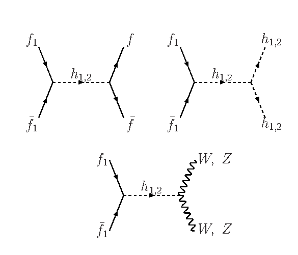
  Figure 1: Feynman diagrams for dark matter annihilation into fermions (quarks and leptons), gauge bosons and scalars contributing to DM annihilation cross-section.

  The DM relic density as measured by PLANCK satellite experiment is given as [2]

  $$\Omega_{\rm DM}h^{2}=0.1199{\pm 0.0027}\,\,.$$ (30)

  In Eq. 30, $h$ is the Hubble parameter measured in the unit of 100 km s^-1 Mpc^-1. We calculate the relic density for the fermionic (SU(2)_H) dark matter candidate in the assumed dark sector in our model by solving the Boltzmann equation. Relic density of the DM candidate is obtained by solving the Boltzmann equation [111]

  $$\frac{{\rm d}n}{{\rm d}t}+3{\rm H}n = -\langle\sigma{\rm v}\rangle(n^{2}-n_{\rm{eq}}^{2})\,\,,$$ (31)

  where $n$ is the number density of DM particle and $n_{\rm eq}$ is the same in equilibrium. In Eq. 31, $\langle\sigma{\rm v}\rangle$ is the thermal averaged annihilation cross-section of DM particle into SM sector and $\rm H$ is Hubble parameter. Solution to Eq. 31 gives the DM relic abundance of the form

  $$\Omega_{\rm{DM}}{\rm h}^{2} = \frac{1.07\times 10^{9}x_{f}}{\sqrt{g_{*}}M_{\rm Pl}\langle\sigma{\rm v}\rangle}\,\,,$$ (32)

  where $g_{*}$ is the effective number of d.o.f (degrees of freedom), $M_{\rm Pl}$ is the PLANCK mass ($\sim 1.22\times 10^{19}$ GeV) and $x_{f}=m/T_{f}$ with $T_{f}$ being the freeze out temperature of the DM species respectively. We compute the freeze out temperature $T_{f}$ by solving iteratively the following equation

  $$x_{f} = \ln\left(\frac{m}{2\pi^{3}}\sqrt{\frac{45M_{\rm{Pl}}^{2}}{2g_{*}x_{f}}}\langle\sigma{\rm v}\rangle\right)\,\,.$$ (33)

  In order to obtain the freeze out temperature of DM and hence its relic density using Eqs. 32, 33 we need to calculate the thermal average of the product between total DM annihilation cross-section ($\sigma$) and the relative velocity (${\rm v}$) of two annihilating DM particles. The expression for the thermally averaged DM annihilation cross-section into all possible final states is given as

  $$\langle\sigma{\rm v}\rangle=\frac{1}{8m^{4}\,T_{f}\,K_{2}^{2}(m/T_{f})}\int_{4m^{2}}^{\infty}ds~{}\sigma(s)~{}(s-4m^{2})\,\sqrt{s}\,K_{1}(\sqrt{s}/T_{f}),$$ (34)

  where the factors $K_{i},~{}(i=1,2)$ are the modified Bessel functions and $\sqrt{s}$ being the centre of mass energy. In the present formalism dark matter candidate $f_{1}$ can annihilate into the SM particles through $s$-channel processes mediated by the scalar bosons $h_{1}$ and $h_{2}$. In the above Eq. 34, $\sigma(s)$ denotes the total annihilation cross-section of dark matter into all possible final states which are allowed by the Lagrangian given in Eq. 10. Feynman diagrams for different annihilation channels of $f_{1}$ are shown in Fig. 1. The expressions of $\sigma{\rm v}$ for different final state annihilation of dark matter into SM particles are derived from the Feynmann diagrams shown in Fig. 1. The value of $\sigma{\rm v}$ obtained for DM annihilation into SM fermion and antifermion pairs ($f\bar{f}$) at the final state is of the form

  $$\sigma{\rm v}_{f\bar{f}} = N_{c}\frac{m^{2}}{v_{s}^{2}}\frac{s_{\alpha}^{2}c_{\alpha}^{2}}{8\pi}\frac{m_{f}^{2}}{v^{2}}\left(1-\frac{4m_{f}^{2}}{s}\right)^{3/2}(s-4m^{2})\left[\frac{1}{(s-m_{1}^{2})^{2}+m_{1}^{2}\Gamma_{1}^{2}}+\frac{1}{(s-m_{2}^{2})^{2}+m_{2}^{2}\Gamma_{2}^{2}}\right.$$ (35)

  $$\left.-\frac{2(s-m_{1}^{2})(s-m_{2}^{2})+2m_{1}m_{2}\Gamma_{1}\Gamma_{2}}{[(s-m_{1}^{2})^{2}+m_{1}^{2}\Gamma_{1}^{2}][(s-m_{1}^{2})^{2}+m_{1}^{2}\Gamma_{2}^{2}]}\right]\,\,,$$

  where $m$ is the DM mass and $m_{f}$ is the mass of specific fermion ($f=$ quark or lepton). In Eq. 35 $v$ and $v_{s}$ are the vacuum expectation values of SM Higgs doublet and dark Higgs doublet, $N_{c}$ is the colour quantum number (3 for quarks and 1 for leptons). Moreover, $\Gamma_{1}$, $\Gamma_{2}$ are the total decay widths of the scalar bosons $h_{1}$, $h_{2}$ and the expressions of $\Gamma_{1}$ and $\Gamma_{2}$ are given in Eqs. 24, 28. We also calculate $\sigma{\rm v}$ for $W^{+}W^{-}$ and $ZZ$ channels which proceed through the $s$-channel exchange of scalar bosons $h_{1}$, $h_{2}$ (see Fig. 1). The expressions of $\sigma{\rm v}_{W^{+}W^{-}}$ and $\sigma{\rm v}_{ZZ}$ are furnished below

  $$\sigma{\rm v}_{W^{+}W^{-}} = \frac{m^{2}}{v_{s}^{2}}\frac{s_{\alpha}^{2}c_{\alpha}^{2}}{8\pi s}\left(1-\frac{4m_{W}^{2}}{s}\right)^{1/2}\left(\frac{2m_{W}^{2}}{v}\right)^{2}\left(1+\frac{(s/2-m_{W}^{2})^{2}}{2m_{W}^{4}}\right)(s-4m^{2})\left[\frac{1}{(s-m_{1}^{2})^{2}+m_{1}^{2}\Gamma_{1}^{2}}\right.$$ (36)

  $$\left.+\frac{1}{(s-m_{2}^{2})^{2}+m_{2}^{2}\Gamma_{2}^{2}}-\frac{2(s-m_{1}^{2})(s-m_{2}^{2})+2m_{1}m_{2}\Gamma_{1}\Gamma_{2}}{[(s-m_{1}^{2})^{2}+m_{1}^{2}\Gamma_{1}^{2}][(s-m_{1}^{2})^{2}+m_{1}^{2}\Gamma_{2}^{2}]}\right]\,\,,$$

  and

  $$\sigma{\rm v}_{ZZ} = \frac{m^{2}}{v_{s}^{2}}\frac{s_{\alpha}^{2}c_{\alpha}^{2}}{16\pi s}\left(1-\frac{4m_{Z}^{2}}{s}\right)^{1/2}\left(\frac{2m_{Z}^{2}}{v}\right)^{2}\left(1+\frac{(s/2-m_{Z}^{2})^{2}}{2m_{Z}^{4}}\right)(s-4m^{2})\left[\frac{1}{(s-m_{1}^{2})^{2}+m_{1}^{2}\Gamma_{1}^{2}}\right.$$ (37)

  $$\left.+\frac{1}{(s-m_{2}^{2})^{2}+m_{2}^{2}\Gamma_{2}^{2}}-\frac{2(s-m_{1}^{2})(s-m_{2}^{2})+2m_{1}m_{2}\Gamma_{1}\Gamma_{2}}{[(s-m_{1}^{2})^{2}+m_{1}^{2}\Gamma_{1}^{2}][(s-m_{1}^{2})^{2}+m_{1}^{2}\Gamma_{2}^{2}]}\right]\,\,.$$

  In the above, $m_{W}$ and $m_{Z}$ denotes the respective masses of $W$ and $Z$ bosons. Annihilations of DM particles into scalar bosons $h_{1}$ and $h_{2}$ are also taken into account. The process of DM annihilation into scalars $h_{1}$ or $h_{2}$ is also scalar mediated, depends on scalar couplings between $h_{1}$ and $h_{2}$. The $s$-channel annihilation cross-section of $f_{1}$ annihilating into the pairs of $h_{1}$ and $h_{2}$, calculated using $f_{1}\bar{f_{1}}\rightarrow h_{i}h_{i},~{}i=1,2$ annihilation diagram, takes the following form

  $$\sigma{\rm v}_{h_{1}h_{1}} = \frac{1}{16\pi s}\frac{m^{2}}{v_{s}^{2}}\left(1-\frac{4m_{1}^{2}}{s}+\frac{4m_{1}^{2}(m_{1}^{2}-1)}{s^{2}}\right)^{1/2}(s-4m^{2})\left[\frac{s_{\alpha}^{2}\lambda_{111}^{2}}{(s-m_{1}^{2})^{2}+m_{1}^{2}\Gamma_{1}^{2}}\right.$$ (38)

  $$\left.+\frac{c_{\alpha}^{2}\lambda_{211}^{2}}{(s-m_{2}^{2})^{2}+m_{2}^{2}\Gamma_{2}^{2}}-\frac{2s_{\alpha}c_{\alpha}\lambda_{111}\lambda_{211}((s-m_{1}^{2})(s-m_{2}^{2})+2m_{1}m_{2}\Gamma_{1}\Gamma_{2})}{[(s-m_{1}^{2})^{2}+m_{1}^{2}\Gamma_{1}^{2}][(s-m_{1}^{2})^{2}+m_{1}^{2}\Gamma_{2}^{2}]}\right]\,\,,$$

  and

  $$\sigma{\rm v}_{h_{2}h_{2}} = \frac{1}{16\pi s}\frac{m^{2}}{v_{s}^{2}}\left(1-\frac{4m_{2}^{2}}{s}+\frac{4m_{2}^{2}(m_{2}^{2}-1)}{s^{2}}\right)^{1/2}(s-4m^{2})\left[\frac{s_{\alpha}^{2}\lambda_{122}^{2}}{(s-m_{1}^{2})^{2}+m_{1}^{2}\Gamma_{1}^{2}}\right.$$ (39)

  $$\left.+\frac{c_{\alpha}^{2}\lambda_{222}^{2}}{(s-m_{2}^{2})^{2}+m_{2}^{2}\Gamma_{2}^{2}}-\frac{2s_{\alpha}c_{\alpha}\lambda_{122}\lambda_{222}((s-m_{1}^{2})(s-m_{2}^{2})+2m_{1}m_{2}\Gamma_{1}\Gamma_{2})}{[(s-m_{1}^{2})^{2}+m_{1}^{2}\Gamma_{1}^{2}][(s-m_{1}^{2})^{2}+m_{1}^{2}\Gamma_{2}^{2}]}\right]\,\,,$$

  where, $\lambda_{ijk}$ is the coupling for the vertex involving three scalar fields $h_{i}h_{j}h_{k}$. The expressions for the scalar couplings $\lambda_{111},~{}\lambda_{211},~{}\lambda_{122}$ and $\lambda_{222}$ are given in Appendix A. We calculate the thermally averaged annihilation cross-section of the present DM candidate using Eqs. 34-39 We then compute the freeze out temperature $T_{f}$ by solving Eq. 33 and finally obtain the relic density of $f_{1}$ at the present epoch from Eq. 32.

• DM Direct Detection - Direct detection of DM particle is based on the scattering of the DM particle with the target nucleus of the detector material. Fermionic dark matter in the present model can undergo elastic scattering with the detector nucleus. This elastic scattering of the DM and the nucleus will transfer a recoil energy to the target nucleus which is then calibrated. From the non-observance of such elastic scattering events the direct detection experiments give the upper bound of elastic scattering cross-sections for different possible masses of dark matter. The scattering cross-section is expressed as cross-section per nucleon for enabling direct comparison of the results from different experiments. In the present model DM fermion of mass $m$ can interact with the target nucleus through t-channel Higgs mediated processes through both $h_{1}$ and $h_{2}$. The spin-independent (SI) elastic scattering cross-section off the detector material normalised to per nucleon can be written as [66]

  $$\sigma_{\rm{SI}}=\frac{\sin^{2}2\alpha}{4\pi}\frac{m^{2}}{v_{s}^{2}}m_{r}^{2}\left(\frac{1}{m_{1}^{2}}-\frac{1}{m_{2}^{2}}\right)^{2}\lambda_{p}^{2}$$ (40)

  where $m_{r}=\frac{mm_{p}}{m+m_{p}}$ is the reduced mass for the DM-nucleon system and $\lambda_{p}$ [66] is given in terms of the form factors $f_{q}$, proton mass $m_{p}$ as

  $$\lambda_{p}=\frac{m_{p}}{v}\left[\sum_{q}f_{q}+\frac{2}{9}\left(1-\sum_{q}f_{q}\right)\right]\simeq 1.3\times 10^{-3}\,\,.$$ (41)

  Using Eqs. 40-41, we calculate the spin independent elastic scattering cross-section of the DM fermion off the nucleon and compare it with the experimental bounds from LUX [9].

  Note that both DM annihilation cross-section and DM-nucleon scattering cross-section depend on an effective coupling $g_{eff}=|\frac{m}{v_{s}}s_{\alpha}c_{\alpha}|$ (Eqs. 35-40). This effective coupling is a useful parameters to explain the dark matter phenomenology in the present framework. Further discussions on the effective coupling are given later in Sec. 4.

• DM Indirect Detection The existence of DM has now been well established from gravitational evidences in astrophysical scale. Indirect search of DM focuses on the non-gravitational search of DM candidate and explores the particle physics nature of DM. The astrophysical sites such as Galactic Centre (GC), dwarf galaxies etc. are of great interest since dark matter can be trapped and accumulate at GC due to the enormous gravity in the region of GC and the mass to luminosity ratio of dwarf galaxies indicate the presence of dark matter in large magnitude. These sites are suitable for indirect search of DM as DM particles trapped in these regions can undergo annihilation into various SM particles which can further produce gamma rays, neutrinos etc. Thus any observed excess in the fluxes of $\gamma$-ray, positron, anti-proton from such sites can indicate DM annihilation processes in those sites if other astrophysical phenomena cannot explain the observed excess. Fermi-LAT [112] searches for the excess emission of $\gamma$-rays originating from GC and dwarf galaxies. Observation of the excess in $e^{+}/e^{-}$ and $p/\bar{p}$ flux is performed by AMS-02 [113] experiment. In this Section we will study Fermi-LAT observed gamma ray flux results from the centre of Milky Way and surrounding dwarf spheroidal galaxies (dSphs).

  The expression for the differential $\gamma$-ray flux obtained from a region of interest (ROI) subtends a solid angle $\rm d\Omega$ centered at GC is given as

  $$\frac{\rm d\Phi}{\rm dEd\Omega}=\frac{1}{8\pi m_{DM}^{2}}J\sum_{f}{\langle\sigma{\rm v}\rangle}_{f}\frac{dN_{f}}{dE_{\gamma}}\,\,,$$ (42)

  where ${\langle\sigma{\rm v}\rangle}_{f}$ is the average thermal annihilation cross-section of DM particles annihilating into final state particle $f$ and $\frac{dN_{f}}{dE_{\gamma}}$ is the photon energy spectrum of DM annihilation into the same. The factor $J$ appearing in Eq. 42 is related to the quantity of dark matter present at the astrophysical site considered and is expressed in terms of dark matter density as

  $$J=\int_{\rm los}\rho^{2}(r(s,\theta))ds\,\,.$$ (43)

  In Eq. 43 the line of sight (los) integral is performed over an angle $\theta$ , is the angular aperture between the line connecting GC to the Earth and the direction of line of sight. In the above Eq. 43, $r=\sqrt{r_{\odot}^{2}+s^{2}-2r_{\odot}s\cos\theta}$ where $r_{\odot}=8.5$ kpc, is the distance to the Sun from GC. It is clear from the expression of Eq. 43 that value of $J$ factor is dependent on the nature of the chosen $\rho(r)$ factor i.e, DM halo density profile $\rho(r)$. In the present work, we consider Navarro-Frenk-White (NFW) [114] halo profile. DM density distribution for the NFW halo profile is given as

  $$\rho(r)=\rho_{0}\frac{(r/r_{s})^{-\gamma}}{(1+r/r_{s})^{3-\gamma}}\,.$$ (44)

  where $r_{s}=20$ kpc is the characteristic distance and $\rho_{0}$ is normalised to local DM density i.e., $\rho_{\odot}=0.4~{}{\rm{GeV~{}cm^{-3}}}$ at a distance $r_{\odot}$ from GC.

  The analysis by Daylan et. al. [21] of Fermi-LAT data suggests an excess in $\gamma$-ray in the $\gamma$ energy range of 2-3 GeV at GC. The same analysis demonstrates that this excess can be explained by the annihilation of 31-40 GeV DM into $b\bar{b}$ with ${\langle\sigma{\rm v}\rangle}_{b\bar{b}}=1.4-2.0\times 10^{-26}~{}{\rm cm}^{3}{\rm s}^{-1}$. In this work [21], inner galaxy gamma ray flux ($5^{0}$ from GC) is calibrated using NFW halo profile with $\gamma=1.26$ and local DM density $\rho_{\odot}=0.3~{}{\rm{GeV~{}cm^{-3}}}$. In a recent work by Calore, Cholis and Weniger (CCW) [22] detailed analysis is performed for the GC $\gamma$-rays along with the systematic uncertainties using 60 galactic diffusion excess (GDE) models. Results from CCW analysis provides a best fit for DM annihilation into $b\bar{b}$ having mass $49^{+6.4}_{-5.4}$ GeV with ${\langle\sigma{\rm v}\rangle}_{b\bar{b}}=1.76^{+0.28}_{-0.27}\times 10^{-26}~{}{\rm cm}^{3}{\rm s}^{-1}$. However, CCW analysis of Galactic Centre excess (GCE) for gamma ray have also considered generalised NFW profile ($\gamma$=1.2, $\rho_{\odot}=0.4~{}{\rm{GeV~{}cm^{-3}}}$) for a different region of interest (ROI) with galactic latitude $|l|\leq 20^{0}$ and longitude $|b|\leq 20^{0}$ masking out inner $|b|\leq 2^{0}$. In another work P. Agrawal et. al. [115] reported that annihilation of heavier dark matter (upto 165 GeV for $b\bar{b}$ channel) can also explain the observed GCE in $\gamma$-ray when uncertainties in DM halo profile (NFW) and the $J$-factor are taken into account. However in the present work, we do not consider any such uncertainties in halo profiles or $J$ vaules and use the canonical NFW halo profile used in CCW analysis. Using Eqs. 42-44, we calculate the $\gamma$-ray flux (in GeV cm^-2 s sr^-1) for the ROI described in CCW analysis for Fermi-LAT data. As mentioned earlier we consider for our calculations the NFW profile with $\gamma=1.2$ and $\rho_{\odot}=0.4~{}{\rm{GeV~{}cm^{-3}}}$.

  Apart from the GC region, dwarf galaxies of the Milky-Way galaxy are also of great significance for indirect search of DM as these galaxies are supposed to be rich in dark matter. Recent analyses of $\gamma$-ray fluxes from 15 Milky-Way dSphs reported by Fermi-LAT [11] provide a limit on DM mass and corresponding thermally averaged annihilation cross-section ${\langle\sigma{\rm v}\rangle}_{f}$ into different channels $f~{}(\tau~{}{\rm and}~{}b)$. Fermi-LAT have used their 6 year data collected by Fermi Large area Telescope and performed an analysis for 15 dSphs using “pass-8 event level analysis“ (see [11] and references therein). In an another work [12] Fermi-LAT in collaboration along with Dark Energy Survey (DES) collaboration also provide similar bound on ${\langle\sigma{\rm v}\rangle}_{f}$ where they include data for 8 new dSphs. For both the analysis presented in [11, 12] a canonical NFW halo profile ($\gamma=1$) is considered, and the astrophysical $J$ factors are measured over a solid angle $\Delta\Omega=2.4\times 10^{-3}~{}{\rm sr}$ with angular radius $0.5^{0}$. Independent searches carried out by Fermi-LAT [11] and DES-Fermi-LAT collaboration on 15 previously discovered and 8 recently discovered different dSphs reported no significant excess in observed $\gamma$-ray. Results from the DES dSphs [12] also predicts an upper bound to the observed $\gamma$-ray energy flux with 95% confidence limit (C.L.) for 8 newly found dSphs. Gamma ray flux for dwarf galaxies when integrated for an energy range extending over a region of solid angle $\Delta\Omega$ is expressed as

  $$\Phi=\frac{{\langle\sigma{\rm v}\rangle}}{8\pi m_{DM}^{2}}J\int_{E_{\rm min}}^{E_{\rm max}}\frac{dN}{dE_{\gamma}}dE_{\gamma}\,\,,$$ (45)

  where $\frac{dN}{dE_{\gamma}}$ is the $\gamma$-ray. The expression of flux presented in Eq. 45 is calculated for a single final state annihilation of DM. Hence, summation over different final channels is not needed. Form of $J$ factor appearing in Eq. 45 is different from Eq. 43 and written as

  $$J=\int_{\Delta\Omega}\int_{\rm los}\rho^{2}(r(s,\theta))ds\,,$$ (46)

  calculated over a solid angle $\Delta\Omega=2.4\times 10^{-3}$ sr subtended by the ROI ($0.5^{0}$ angular radius) for NFW halo profile ($\gamma=1$). The density distribution function for NFW profile with $\gamma=1$ is then

  $$\rho(r)=\rho_{0}\frac{r_{s}^{3}}{r(r_{s}+r)^{2}}\,,$$ (47)

  where $r_{s}$ is the NFW scale radius and $\rho_{0}$ represents the characteristic density for the dSphs. In the case of Fermi-LAT analysis, $J$ factors for different dSphs are adopted from Ref. [11]. We use values of $J$ factor from [12] for computing gamma ray flux for 8 DES dSphs for the dark matter candidates in our model. However, it is to be noted that $J$ factors for DES dSphs candidates are obtained assuming the point like dSphs instead of having spatial extension (as in the case of [11]) to avoid the uncertainties in halo profile arising from spatial extension. Calculation of gamma ray flux is also based on the assumption that the spectrum $\frac{dN}{dE_{\gamma}}$ follows the conventional power law $\frac{dN}{dE_{\gamma}}\sim\frac{1}{E^{2}}$. As mentioned earlier, study of 15 dSphs by Fermi-LAT and 8 other dSphs by DES-Fermi-LAT collaboration found no significant excess in $\gamma$-ray from these dwarf galaxies. However, a recent search on a newly discovered dwarf galaxy Reticulum 2 (Ret2) in a work by Geringer-Sameth et. al [10] has reported an excess in observed $\gamma$-ray signal. In the present work, we calculate the $\gamma$-ray flux for annihilation of hidden SU(2)_H fermionic dark matter into $\gamma$-ray through different SM final states and explore whether the model can account for GCE in $\gamma$-ray and also satisfies the bounds on gamma ray flux from dwarf satellite galaxies.

  As mentioned earlier, in the present model dark matter candidate ($f_{1}$) is fermionic in nature and it interacts with the visible world (SM particles) through the exchange of two real scalar bosons $h_{1}$ and $h_{2}$. As a result the annihilation cross-sections of the DM dark candidate $f_{1}$ into the final states that composed of SM particles (mainly light quarks and leptons) are proportional to the square of relative velocity (${\rm v}^{2}$) between the annihilating dark matter particles (p wave process). Now the averaged DM relative velocity is proportional to $\sim\sqrt{3/x}$ [116]-[117] with $x=\frac{m}{T}$ is a dimensionless quantity and $T$ being the temperature of the Universe. Hence, in our model, the thermally averaged annihilation cross-section used for computing DM relic density, at $x\sim 20-30$, is different from the annihilation cross-section (for $x\sim 3\times 10^{6}$ [116]-[117]) needed to calculate $\gamma$-ray flux at the Galactic Centre and dwarf galaxies. The latter quantity is velocity suppressed as the average DM relative velocity is $\sim 10^{-3}$ when the annihilation of DM occurs at the GC. Among all the annihilation channels of $f_{1}$, the annihilation mode $f_{1}\bar{f_{1}}\rightarrow b\bar{b}$ plays a significant role for the $\gamma$-ray excess observed from GC and dwarfs satellite galaxies as it is the most dominant annihilation channel for the considered mass range of DM. In order to explain the GC gamma-excess by DM annihilation to $b\bar{b}$, the annihilation cross-section should be $\sim 1.76^{+0.28}_{-0.27}\times 10^{-26}$ cm${}^{3}/$s [22]. Although in the present case, the thermally averaged annihilation cross-section for the $b\bar{b}$ annihilation is quite small, however the quantity $\langle{\sigma{\rm v}}\rangle_{b\bar{b}}$ can be significantly enhanced using Breit-Wigner resonant enhancement mechanism [116]-[117]. Breit-Wigner enhancement occurs only when the mass of the dark matter ($m$) is nearly equal to half of the mediator mass (in our case it is the mass of $h_{2}$). Therefore, we have defined the mass of the hidden sector scalar boson ($h_{2}$) and the centre of mass energy $\sqrt{s}$ in the following way

  $$m^{2}_{2}=4m^{2}(1-\delta)\,\,{\rm and}\,\,s=4m^{2}(1+z)\,\,,$$ (48)

  where $\delta<0$ represents the physical pole and $z$ is the measure of excess centre of momentum energy scaled by $4m^{2}$. In terms of $z$, Eq. 34 for the $b\bar{b}$ annihilation channel, can now be written as

  $${\langle{\sigma{\rm v}}\rangle}_{b\bar{b}}=\frac{4\,x}{K^{2}_{2}(x)}\int^{z_{eff}}_{0}dz\,\sigma(z)_{b\bar{b}}\,z\,\sqrt{1+z}\,K_{1}(2\,x\,\sqrt{1+z})$$ (49)

  with the expression of $\sigma(z)_{b\bar{b}}$ is given by

  $$\sigma(z)_{b\bar{b}}=\frac{g_{c}}{4m^{2}}\,\frac{\sqrt{z}}{1+z}\,\frac{\left(1+z-\frac{m^{2}_{b}}{m^{2}}\right)^{3/2}}{\left[(z+\delta)^{2}+\gamma^{2}_{2}(1-\delta)^{2}\right]}\,\,,$$ (50)

  and

  $$g_{c}=\frac{N_{c}}{16\,\pi}\,\left(\frac{m\cos\alpha}{v_{s}}\frac{m_{b}\sin\alpha}{v}\right)^{2}\,$$ (51)

  where $\gamma_{2}=\frac{\Gamma_{2}}{m_{2}}$, $\Gamma_{2}$ being the total decay width of $h_{2}$ of mass $m_{2}$. It is to be noted that the upper limit of the above integration should be $\infty$ (see Eq. 34), however the integrand becomes negligibly small when $z$ approaches to $z_{eff}\sim{\rm max}[4/x,\,2|\delta|]$ for $\delta<0$ [37],[117]. Using the above prescription, we calculate the thermally averaged annihilation cross-section $\langle{\sigma{\rm v}}\rangle_{b\bar{b}}$ of the dark matter candidate $f_{1}$ for GC and dwarf spheroidal galaxies. The actual values of $\langle{\sigma{\rm v}}\rangle_{b\bar{b}}$, $\gamma_{2}$ and $\delta$ for the two chosen bench mark points (BP1, BP2) are given in Table 1 of Sec. 4. We have found that for $|\delta|\sim 10^{-3}$ the annihilation cross-section $\langle{\sigma{\rm v}}\rangle_{b\bar{b}}\sim 1.9\times 10^{-26}$ cm${}^{3}/$s which can explain the excess of gamma ray flux in GC.

4 Calculational procedures and Results

In this section we present the computation of dark matter annihilation cross-sections as also the DM-nucleon elastic scattering cross-sections. They are required for the calculation of relic densities and the comparison of the latest DM scattering cross-section bound given by the LUX direct detection experiment. The invisible decay widths and signal strengths for the SM-like scalar is also calculated in order to constrain the model parameter space. The gamma ray flux are then computed within the framework of SU(2)_H fermionic dark matter for galactic centre as also for dwarf galaxies and the results are compared with the experimental analysis.

4.1 Constraining the model parameter space

The fermionic dark matter in the present model can annihilate through scalar mediated ($h_{1}$ and $h_{2}$) $s$-channel processes. As mentioned in Sec. 3, the model parameter space is first constrained by the vacuum stability conditions given in Eq. 20. The signal strengths $R_{1}$ and $R_{2}$ for the Higgs doublets $h_{1}$ (SM) and $h_{2}$ (dark sector) are then computed using Eqs. 30-34. With the chosen constraints on $R_{1}$ ($R_{1}\geq$ 0.8, Ref. [109]) the invisible decay branching ratio of SM-like Higgs ${\rm Br}^{1}_{\rm inv}$ is calculated and the parameter space is further constrained by LHC experiment limit of ${\rm Br}^{1}_{\rm inv}$ (${\rm Br}^{1}_{\rm inv}\leq~{}0.2$ [70]). The parameter space thus constrained is then used to compute the thermal averaged annihilation cross-section ${\langle\sigma{\rm v}\rangle}$ of the present fermionic dark matter candidate and the relic density is obtained by solving the Boltzmann equation (using Eqs. 31- 34). The annihilation cross-sections are computed with the calculated analytical formulae given in Eqs. 35-39 with two choices of VEV for $\Phi$ (dark Higgs doublet) namely $v_{s}=$ 246 GeV and 500 GeV. In our calculation we consider the mass $m_{1}$ of the SM-like Higgs boson $h_{1}$ to be 125 GeV. The calculation is performed for two values of the dark sector scalar $h_{2}$ masses and they are $m_{2}=$ 100 GeV and 110 GeV. These relic densities are compared with the dark matter relic density given by PLANCK [2]. Thus PLANCK result further constrains the parameter space of our model. With this available parameter space we evaluate the dark matter-nucleon spin independent scattering cross-section ($\sigma_{\rm SI}$) for the purpose of comparing our results with those given by the dark matter direct detection experiments such as LUX, XENON100 etc. In this way we restrict our model parameter space by different experimental results.

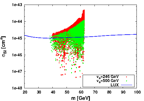
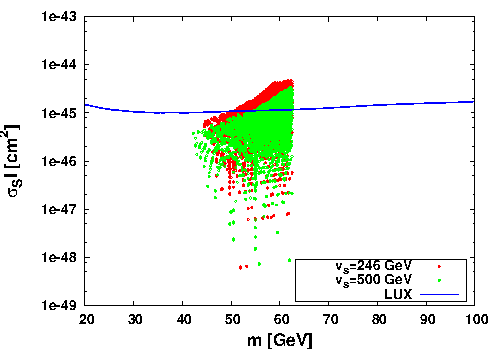
Figure 2: The allowed range of $m-\sigma_{\rm SI}$ parameter space obtained for $m_{2}=$ 100 GeV (left panel) and $m_{2}=$ 110 GeV (right panel) plotted using the bounds from vacuum stability, LHC constraints on SM Higgs and relic abundance of DM obtained from PLANCK [2]. Limits on DM-nucleon cross-section from LUX [9] is also plotted (blue line) for comparison.

In Fig. 2a and Fig. 2b we show the calculated values of $\sigma_{\rm SI}$ with different DM mass in the present model where the conditions from vacuum stability, bound on SM Higgs signal strength and DM relic density results from PLANCK have been imposed. We first choose certain values of $m_{1}$ and $m_{2}$ and vary the couplings $\lambda_{i},~{}i=1$ to $3$ (satisfying vacuum stability conditions given in Eq. 20) for two different values of $v_{s}$ which also constrain the mixing angle $\alpha$ through the Eq. 18. Here we want to mention that we have varied $\lambda_{1}$ and $\lambda_{2}$ in the range 0 to 0.2 with the values of both $\lambda$’s are evenly spread within the considered range. Consequently the value of the parameter $\lambda_{3}$ becomes fixed by the vacuum stability criteria given in Eq. 20 which is also varied with equal interval in the range $|\lambda_{3}|<2\sqrt{\lambda_{1}\lambda_{2}}$. The model parameter space thus obtained is then further constrained by imposing the conditions $R_{1}>0.8$ and $Br^{1}_{\rm inv}<0.2$ from LHC results. Using this restricted model parameter space satisfying both vacuum stability and LHC bounds, we therefore calculate the relic density of the dark matter candidate $f_{1}$ by solving the Boltzmann equation (Eq. 31) for different values of DM mass. Finally, we consider specific range of model parameter space which is in agreement with DM relic density reported by PLANCK experiment and for these parameter space we compute the spin-independent direct detection cross-section using Eqs. 40-41. In this way the viable model parameter space for the dark matter candidate $f_{1}$ is obtained. Fig. 2a is for the case $m_{2}=$ 100 GeV while Fig. 2b is for the case $m_{2}=$ 110 GeV. The upper limit on $\sigma_{\rm SI}$ for different values of DM mass, obtained from LUX DM direct search experiment, are also shown in Fig. 2a-b by the blue line for comparison. The red and green scattered regions as shown in Fig. 2a-b correspond to two choices of $v_{s}$=246 GeV and 500 GeV respectively. From Fig. 2a it can be observed that only the region near the resonances of scalar bosons $h_{1}$ and $h_{2}$ is in agreement with the upper limit on $\sigma_{\rm SI}$ predicted by LUX. It is also seen from Fig. 2a that the choice of $v_{s}$ do not alter the allowed range of parameter space. Observation of Fig. 2b yields that, apart from SM Higgs resonance region ($m\sim m_{1}/2$) there exists another allowed range of $m-\sigma_{\rm SI}$ parameter space in the vicinity of non-SM scalar resonance ($m\sim m_{2}/2$). Note that variation of $m$ with $\sigma_{\rm SI}$ depicted in Fig. 2b depends only on the masses of scalar bosons and does not suffer any significant change due to change in $v_{s}$. The non-SM Higgs signal strength $R_{2}$ (calculated using Eq. 27) for the valid $m-\sigma_{\rm SI}$ parameter space shown in Figs. 2a-b is very small and $R_{2}<0.2$.

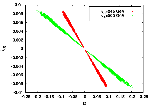
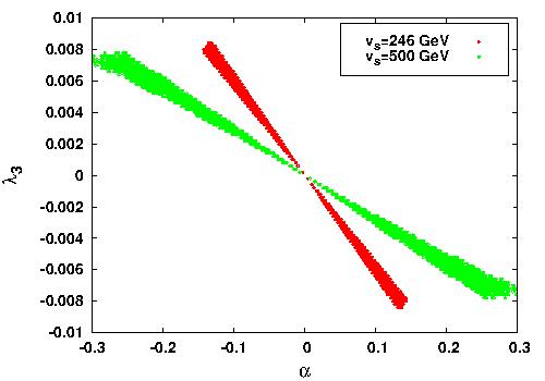
Figure 3: The valid model parameter space in $\lambda_{3}-\alpha$ (in deg) plane obtained for the case of $m_{2}=100$ GeV (lef panel) and $m_{2}=$ 110 Gev (right panel) satisfying the limits from vacuum stability, LHC findings, PLANCK DM relic abundance and direct detection limits on $\sigma_{\rm SI}$ from LUX experiment.

In this work, we assumed two values for VEV $v_{s}$ (246 GeV and 500 GeV) for the hidden sector Higgs doublet $\Phi_{\rm HS}$. From Eq. 2, we observe that the mixing between the scalars $h_{1}$ and $h_{2}$ depends on the VEV of $\Phi_{\rm HS}$ and $H$. Hence, the choice of $v_{s}$ may change the range of available model parameter space. In Figs. 3a-b, we plot the variation of Higgs mixing angle $\alpha$ between $h_{1}$ and $h_{2}$ with $\lambda_{3}$ for $m_{2}$=100 GeV and 110 GeV with $m_{1}$=125 GeV (mass of SM-like Higgs). Needless to mention the region of $\alpha-\lambda_{3}$ space shown in Figs. 3a-b are consistent with the bounds form vacuum stability, SM Higgs signal strength from LHC, relic abundance of DM from PLANCK and limits on DM-nucleon scattering cross-section from LUX direct DM search experiment. Plots in Fig. 3 are produced using similar method we have applied previously to obtain viable model parameter space for Fig. 2. However $\alpha-\lambda_{3}$ plane in Fig. 3 is further constrained by imposing LUX DM direct detection bound. The plots in Fig. 3a are for the case when $m_{1}=$ 125 GeV and $m_{2}=$ 100 GeV while plots in Fig. 3b represent the allowed $\alpha-\lambda_{3}$ parameter space when $m_{2}=$ 110 GeV for the fixed value of $m_{1}=125$ GeV. The green and blue regions in Fig. 3a and Fig. 3b correspond to two different values for VEV of dark Higgs doublet, $v_{s}=$ 246 GeV and $v_{s}=$ 500 GeV respectively. From Fig. 3a ($m_{2}=$ 100 GeV case) one observes that for both the considered values of VEV $v_{s}$, the mixing parameter $\lambda_{3}$ remains small and is confined within the region $|\lambda_{3}|<0.01$. For the case when $v_{s}=$246 GeV (the red region of Fig. 3a), the limit of mixing angle $\alpha$ ranges between $-0.1$ to $0.1$. However these range (of mixing angle) varies within the limit $|\alpha|\leq 0.2$ when $v_{s}$=500 GeV is chosen (green region shown in Fig. 3a). Study of the $\lambda_{3}-\alpha$ plots in Fig. 3b (plotted for $m_{2}=$ 110 GeV) reveals that for both the values of $v_{s}$ considered in Fig. 3, the mixing parameter is small ($|\lambda_{3}|<0.01$). The mixing angle $\alpha$ is bounded in the range $|\alpha|<0.15$ and $|\alpha|\leq 0.30$ for $v_{s}=$ 246 GeV and 500 GeV respectively.

4.2 Calculation of gamma ray signals from galactic centre and dwarf galaxies

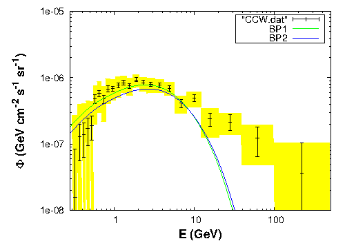
Figure 4: Comparison of the GC $\gamma$-ray flux data from [22] with those calculated for benchmark points in Table 1.

BP	$v_{s}$	$m_{2}$	$m$	$\delta$	$\gamma_{2}$	$\sigma_{SI}$	$\langle\sigma{\rm v}\rangle_{b\bar{b}}$
	in GeV	in GeV	in GeV			in cm2	cm3/s
BP1	246.0	100.242	50.0	-4.86e-03	0.60e-06	2.89e-46	1.98e-26
BP2	500.0	110.321	55.0	-5.85e-03	0.43e-06	1.13e-46	1.90e-26

Table 1: Benchmark points obtained from the constrained model parameter space in agreement with the bounds from vacuum stability, SM Higgs signal strength from LHC, DM relic density from PLANCK and LUX DM serach bounds on DM-nucleon scattering cross-section.

In this Section, we calculate the $\gamma$-ray flux from the galactic centre and dwarf galaxies for the fermionic dark matter in framework of the present model and compare our results with the experimental observations. For these calculations we consider two benchmark points (BPs) from the restricted parameter space that satisfy both theoretical and experimental bounds (mainly vacuum stability, LHC constraints on SM Higgs signal, PLANCK results for relic abundance and direct detection limit on $m-\sigma_{\rm SI}$ from LUX) for two choices of $h_{2}$ mass, mainly, $m_{2}$= 100 GeV and 200 GeV. In Table 1 we tabulate the chosen BPs along with model parameters. There are two chosen sets of benchmark points in Table 1 and we denote them as BP1 and BP2. The GC gamma ray flux is calculated using Eqs. 42-44 for the BPs tabulated in Table 1. The annihilation cross-section $\langle\sigma{\rm v}\rangle_{b\bar{b}}$ for the dark matter particle is calculated using Breit-Wigner enhancment technique using Eqs. 48-51 discussed in Sec. 3. The gamma ray spectrum $\frac{dN}{dE}$ in Eq. 42 is obtained from Ref. [118] for annihilation of DM into any specific channel. The gamma ray spectra for BP1 and BP2 are then calculated for the specified region of interest adopted from Ref. [22] ($|l|\leq 20^{0},~{}2^{0}\leq|b|\leq 20^{0}$) using NFW halo profile (with $\gamma=1.2$, $\rho_{\odot}=0.4~{}{\rm{GeV~{}cm^{-3}}}$). In Fig. 4, we show the calculated GC gamma ray flux (in GeV cm^-2 sr^-1) for our proposed DM candidate with BP1 and BP2. We also show in Fig. 4 the CCW data for comparison. Green and blue lines in Fig. 4 represent the calculated $\gamma$-ray spectra for BP1 and BP2 respectively. Both the benchmarks points are in agreement with the findings from GC gamma ray study presented in CCW [22]. From Fig. 4 it can be observed that flux calculated using the set BP1 ($m$=50 GeV) is in better agreement with the findings from CCW analysis.

We now further investigate how well the DM candidate in our model can explain the observed extragalactic $\gamma$-ray signatures from various dwarf galaxies. From their six years observations on 15 dwarf galaxies, the Fermi-LAT experiment did not obtain any significant excess of $\gamma$-rays. Fermi-LAT collaboration [11] however in a recent work provides combined bound on DM mass and thermally averaged DM annihilation cross-section into SM particles for these 15 dSphs. A similar bound in $m-{\langle\sigma{\rm v}\rangle}_{f}$ plane is also presented recently in an another work [12] for eight new dSphs jointly by Fermi-LAT and DES collaboration. In this work we calculate thermally averaged annihilation cross-section of DM annihilating into SM sector in our model and compare them with experimental results given by [11, 12]. In Fig. 5, we plot the bounds on DM annihilation cross-section ${\langle\sigma{\rm v}\rangle}_{b\bar{b}}$ (for the annihilation channel DMDM$\rightarrow b\bar{b}$) with dark matter mass $m$ obtained from galactic [22] and extragalactic [11, 12] $\gamma$-ray search experiments. We calculate the variations of the same plotted in Fig. 5 for the benchmark points BP1 (for $m_{2}=$ 100 GeV) and BP2 (for $m_{2}=$ 110 GeV) considered in our model.

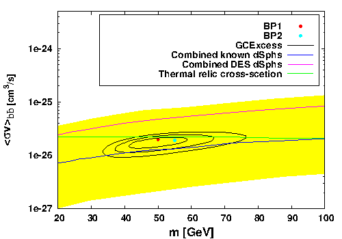
Figure 5: The allowed range of $m-{\langle\sigma{\rm v}\rangle}$ space (for annihilation into $b\bar{b}$) along with the bounds on ${\langle\sigma{\rm v}\rangle}$ (into $b\bar{b}$ channel only) obtained from GC $\gamma$ ray search results CCW [22] and dwarf galaxies [11, 12] compared with the same obtained from benchmark points in Table 1.

Black contours shown in Fig. 5 are the 1$\sigma$, 2$\sigma$ and 3$\sigma$ contours given by the CCW [22] analysis of GC gamma ray excess observations. The blue line in Fig. 5 describes the bounds in $m-{\langle\sigma{\rm v}\rangle}_{b\bar{b}}$ plane given by the analysis of gamma rays from previously discovered 15 dSphs and they are adopted from [11]. Also shown in Fig. 5, the yellow band which is the 95% confidence limit (C.L.) region adopted from the analysis in Ref. [11] for DM annihilation into $b\bar{b}$. The combined bounds on ${\langle\sigma{\rm v}\rangle}_{b\bar{b}}$ for different DM mass $m$ from a recent study of the newly discovered 8 DES dwarf galaxies [12] are given by the pink coloured line in Fig. 5. The green horizontal line in Fig. 5 shows the annihilation cross-section for thermal dark matter that may yield the right DM relic abundance obtained from the PLANCK experiment.

From Fig. 5 one readily observes that the calculated values of ${\langle\sigma{\rm v}\rangle}_{b\bar{b}}$ for the benchmark points BP1 and BP2 in our model broadly agrees with the 1$\sigma$, 2$\sigma$ and 3$\sigma$ allowed regions in $m-{\langle\sigma{\rm v}\rangle}_{b\bar{b}}$ plane obtained from the experimental results. This can also be noted from Fig. 5 that these benchmark points are consistent the combined limit from DES dwarf satellite data and falls within the 95% C.L. limit predicted by Fermi-LAT for 15 dSphs. Also the calculated values of ${\langle\sigma{\rm v}\rangle}_{b\bar{b}}$ for the benchmark points considered in our work lie below the upper bound on thermal DM annihilation cross-section. Hence, DM fermion in the present model can account for the galactic centre excess in $\gamma$-ray and is also consistent with the bounds on gamma ray flux from Milky-Way dwarf satellite galaxies.

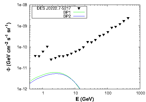
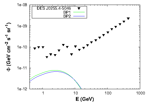
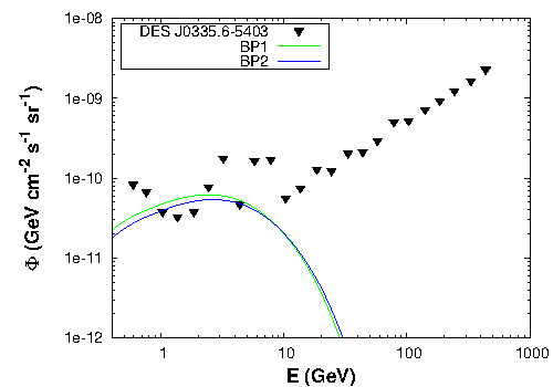
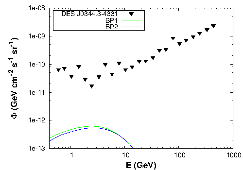
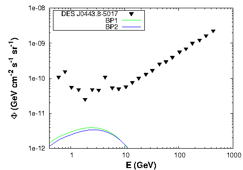
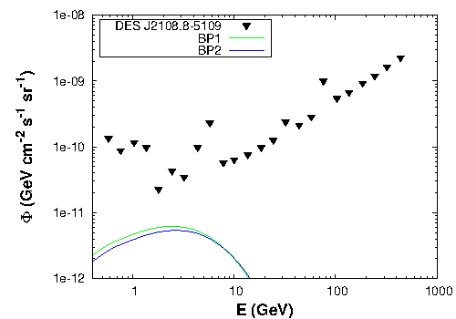
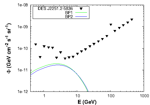
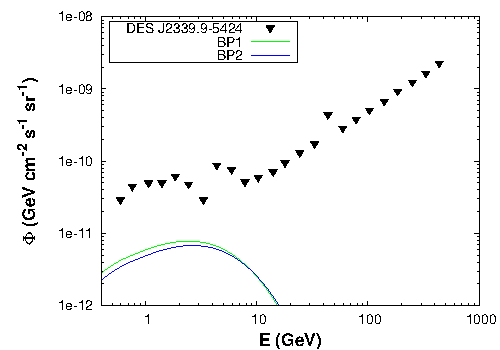
Figure 6: Comparison of the observed upper bound on $\gamma$-ray flux for 8 DES dSphs with the calculated $\gamma$-ray flux from BP1 and BP2 tabulated in Table 1.

We now calculate the gamma ray flux for 8 new dwarf satellite galaxies discovered by the DES experiment for the hidden sector fermionic dark matter candidate proposed in this work. These calculations are performed with each of the benchmark parameter sets BP1 and BP2 given in Table 1. The Gamma ray flux for each of these 8 dSphs in the work [12] is computed using Eq. 45 and the values of the $J$ factors (Eq. 46) for each of the eight dSphs adopted from Ref. [12]. In Ref. [12] these $J$ factors are estimated by integrating the dark matter density (adopting NFW halo profile for DM density distribution) along the line of sight over a solid angle $\Delta\Omega=2.4\times 10^{-4}$ sr^-1. As previously mentioned the gamma ray spectrum $\frac{dN}{dE}$ is also obtained from Ref. [118] for this calculation. The calculated flux for each of the eight dSphs are shown in eight plots (a-h) of Fig. 6. Also shown in each of the eight plots of Fig. 6, the respective upper bounds of the flux given by the experimental observations of gamma rays from each of the eight dSphs. These are shown as red coloured points while the computed flux in this work for the respective dSphs are given by continuous lines in Fig. 6. The green and blue continuous lines in each of the plots (a-h) of Fig. 6 correspond to the calculated flux using the benchmark points BP1 and BP2 respectively. It is clear from Fig. 6 that the fluxes calculated, assuming the annihilation of the DM candidate in our proposed model, for all the eight dSphs do not exceed the upper limit of $\gamma$ flux set by the experimental observations of DES collaboration.

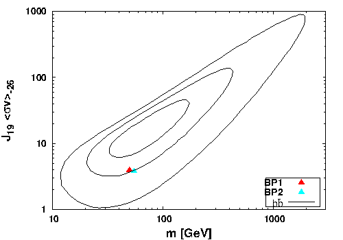
Figure 7: Benchmark points BP1 and BP2 compared with the allowed region of model parameter space shown in $m-J_{19}\langle\sigma{\rm v}\rangle_{-26}$ plane obtained from [10]

Besides the 15 dwarf galaxies investigated earlier and the eight other recently explored dwarf galaxies, one more dwarf galaxy namely Reticulum 2 (Ret2) has been probed very recently. Geringer-Sameth et. al. [10], after an analysis of observed gamma rays from Ret2 dwarf galaxy reported an excess of gamma ray emission from Ret2. From their analysis of Ret2 data Geringer-Sameth et. al. provide different C.L. allowed contours in $m-J_{19}\langle\sigma{\rm v}\rangle_{-26}$ plane where $m$ is the mass of the dark matter and $J_{19}\langle\sigma{\rm v}\rangle_{-26}$ is the product of the $J$ factor in the units of $10^{19}$ GeV² cm^-5 and thermal averaged product $\langle\sigma{\rm v}\rangle$ of annihilation cross-section and relative velocity in the units of $10^{-26}{\rm cm^{3}s^{-1}}$ for various final state SM channels. As mentioned earlier in this work DM candidate primarily annihilates into $b\bar{b}$, only the contours for the DM pair annihilation into $b\bar{b}$ channel are adopted. For the present dark matter model with the constrained parameter space discussed earlier we compute the quantity $J_{19}\langle\sigma{\rm v}\rangle_{-26}$ for different dark matter mass $m$ annihilating into $b\bar{b}$ channel. However the value of the $J$ factor for Ret2 has been adopted from [10]. In their work Geringer-Sameth et. al. [10] estimated the $J$ values by performing line of sight integral over a circular region with angular radius $0.5^{0}$ surrounding the dwarf and over a solid angle $\Delta\Omega=2.4\times 10^{-4}$ sr^-1. All these calculations are performed for two values of non-SM scalar mass accounted in the present model namely $m_{2}=$ 100 GeV and $m_{2}=$ 110 GeV. The results are presented for the two benchmark points BP1 and BP2 corresponding to the calculations with $m_{2}=$ 100 GeV and $m_{2}=$ 110 GeV are shown in red and skyblue points in Fig. 7. In Fig. 7, the contours from the experimental data analysis by Geringer-Sameth et. al. are given for comparison. In Fig. 7 the contours for 68%, 95% and 99.7% C.L. are shown in black coloured lines in increasing order of area enclosed by each contour. The valid regions of $m-J_{19}\langle\sigma{\rm v}\rangle_{-26}$ plane in our model (calculated for DM annihilating into $b\bar{b}$ pair) are presented by green coloured patches in both the plots of Fig. 7. From Fig. 7, it can be easily observed that $J_{19}\langle\sigma{\rm v}\rangle_{-26}$ in the present model calculated for DM annihilating into $b\bar{b}$ channel (for benchmark points with $m_{2}$=100 GeV and 110 GeV) is within the $3\sigma$ C.L. limit. Hence fermionic DM candidate in the present framework can also explain the observed excess in $\gamma$-ray from Ret2.

5 Discussions and Conclusions

In this work, we have proposed the existence of a hidden sector which obeys a local SU(2)_H and a global U(1)_H gauge symmetries. In order to introduce fermions which are charged under this ${\rm SU}(2)_{\rm H}$ gauge group one should have at least two fermion doublets in order to avoid “Witten anomaly”. The particle and the antiparticle of these dark fermions are different as they possess equal and opposite U(1)_H charges. Similar to the usual Higgs doublet in the visible sector, this hidden sector also has an SU$(2)_{\rm H}$ scalar doublet $\Phi$ which however does not have any U(1)_H charge. The ${\rm SU}(2)_{\rm H}$ gauge symmetry breaks spontaneously when the neutral component of the scalar doublet $\Phi$ gets a VEV and thereby generates masses of all the dark gauge bosons ($A^{\prime}_{\mu}$) and dark fermions ($f_{i}$). Since the dark sector fermions interact among themselves through the dark gauge bosons, therefore all the heavier fermions as well as the dark gauge bosons can decay into the lightest fermion and hence the lightest fermion in this dark sector can be treated as a particle for the viable dark matter candidate. In fact in this model this lightest fermion is the only dark matter candidate. The dark fermions and dark gauge bosons do not mix with the SM fermions and gauge bosons due to the non abelian nature of two SU(2) groups. However, the dark sector scalar field can interact with the SM Higgs like scalar in the visible sector and only through this interaction two sectors are mutually connected.

We therefore test the viability of the present model by using theoretical and experimental constraints on the relevant model parameters, such as vacuum stability conditions, bounds on relic abundance of DM from PLANCK experiment, direct detection limits on DM-nucleon scattering cross-section from LUX experiment. LHC bounds on signal strength and invisible decay width of the SM Higgs, are also used to constrain the parameter space. From such analyses we find that only a small region of the parameter space near the scalar resonances (when $m\simeq\frac{m_{1}}{2}$ and $\frac{m_{2}}{2}$), is consistent with the current experimental bounds. Study of the model parameters, thus constrained, shows that the mixing between the two scalars ($h_{1}$, $h_{2}$) of the model is very small (mixing angle $\alpha\leq 0.3$ deg) and depends on the VEV of the dark scalar doublet ($\Phi$). With the allowed regions of parameter space, thus obtained, for the present DM candidate (dark fermion $f_{1}$) we compute the gamma ray flux from the GC region. While calculating the gamma ray flux from GC we have used Breit-Wigner enhancement mechanism for the computation of DM annihilation cross-section into the $b\bar{b}$ final state ($f_{1}\bar{f_{1}}\rightarrow b\bar{b}$). These computational results are then compared with the experimental analyses of the Fermi-LAT GC gamma ray flux data considering the dark matter at the GC primarily pair annihilates into $b\bar{b}$ channel. Our proposed DM candidate can indeed explain the results from these experimental analyses.

In search of indirect evidence of dark matter from astrophysical sources, the gamma rays from various dwarf satellite galaxies are also explored for possible signature of excess gamma rays from these sites. To this end 15 such dwarf galaxies have earlier been investigated and more recently the gamma ray observation is also reported from eight more newly discovered dSphs. From the analyses of these observational results different C.L. bounds have been given in the parameter space of ${\langle\sigma{\rm v}\rangle}_{b\bar{b}}-m$ plane. We compare our computational results with these experimental bounds and found that the $\gamma$-rays that the DM candidate in our model produce on pair annihilation can simultaneously satisfy the observational results from GC and dwarf galaxies. We also demonstrate that the calculated fluxes in our model for each of the recently discovered eight dwarf galaxies lie below the corresponding upper limits of the fluxes obtained from the observational results of these dwarf galaxies. We further demonstrate that our calculations are also in good agreement with the analysis of Ret2 dwarf galaxy observations.

Our work clearly demonstrate that the dark matter candidate proposed in this work is a viable one to explain the $\gamma$-rays from both the GC region and dwarf galaxies simultaneously. However the dark matter can also pair annihilate into fermion-antifermion pairs and there are experiments such as AMS-02 that look for the excess of $e^{+}/e^{-}$ or $p\bar{p}$ in cosmos. In a recent work, AMS-02 collaboration have reported their first measurement of $p/\bar{p}$ flux [119]. A model independent analysis of this AMS-02 $p/\bar{p}$ data is performed by Jin et.al. [120]. In this work [120], the upper limits in $\langle\sigma{\rm v}\rangle$ value for DM annihilation into SM particles (quarks and gauge bosons) for different considered DM halo profiles (NFW, Isothermal, Moore) are obtained. The analysis presented in the work [120] also considered four different propagation models namely conventional, MED, MIN and MAX. We have also checked that the DM in our model satisfies upper bound on $\langle\sigma{\rm v}\rangle_{b\bar{b}}$ given in Ref. [120] when NFW profile is considered. This is found to be true for both the cases of dark sector scalar mass $m_{2}=$ 100 GeV and $m_{2}=$ 110 GeV. Hence, fermionic dark matter explored in the present model can serve as a potential candidate for dark matter. Upcoming results from LHC as also DM direct and indirect search experiments may provide stringent limits on the available model parameter space.

Acknowledgments : A.D. Banik and A. Biswas would like to thank P.B. Pal for useful discussions. A.D.B. and A.B. also acknowledge the Department of Atomic Energy, Govt. of India for financial support.

Appendix A Coupling between the scalars $h_{1}$ and $h_{2}$ are given as follows

$$\lambda_{111}=\lambda_{1}vc_{\alpha}^{3}-\lambda_{2}v_{s}s_{\alpha}^{3}+\frac{1}{2}\lambda_{3}(vc_{\alpha}s_{\alpha}^{2}-v_{s}s_{\alpha}c_{\alpha}^{2})\,,$$

$$\lambda_{222}=\lambda_{1}vs_{\alpha}^{3}+\lambda_{2}v_{s}c_{\alpha}^{3}+\frac{1}{2}\lambda_{3}(vs_{\alpha}c_{\alpha}^{2}+v_{s}c_{\alpha}s_{\alpha}^{2})\,,$$

$$\lambda_{211}=3(\lambda_{1}vc_{\alpha}^{2}s_{\alpha}-\lambda_{2}v_{s}s_{\alpha}^{2}c_{\alpha})+\frac{1}{2}\lambda_{3}(v_{s}(c_{\alpha}^{3}-2s_{\alpha}^{2}c_{\alpha})+v(s_{\alpha}^{3}-2c_{\alpha}^{2}s_{\alpha}))\,,$$

$$\lambda_{122}=3(\lambda_{1}vs_{\alpha}^{2}c_{\alpha}-\lambda_{2}v_{s}c_{\alpha}^{2}s_{\alpha})+\frac{1}{2}\lambda_{3}(v_{s}(-s_{\alpha}^{3}+2c_{\alpha}^{2}s_{\alpha})+v(c_{\alpha}^{3}-2s_{\alpha}^{2}c_{\alpha}))\,.$$

References

- [1] G. Hinshaw et al. [WMAP Collaboration], Astrophys. J. Suppl. 208, 19 (2013) [arXiv:1212.5226 [astro-ph.CO]].
- [2] P. A. R. Ade et al. [Planck Collaboration], Astron. Astrophys. 571, A16 (2014) [arXiv:1303.5076 [astro-ph.CO]].
- [3] R. Agnese et al. [CDMS Collaboration], Phys. Rev. D 88, 031104 (2013).
- [4] R. Agnese et al. [CDMS Collaboration], [Phys. Rev. D 88, no. 5, 059901 (2013)] [arXiv:1304.3706 [astro-ph.CO]].
- [5] R. Agnese et al. [CDMS Collaboration], Phys. Rev. Lett. 111, no. 25, 251301 (2013) [arXiv:1304.4279 [hep-ex]].
- [6] R. Agnese et al. [SuperCDMS Collaboration], [arXiv:1504.05871 [hep-ex]].
- [7] C. E. Aalseth et al. [CoGeNT Collaboration], Phys. Rev. Lett. 106, 131301 (2011) [arXiv:1002.4703 [astro-ph.CO]].
- [8] E. Aprile et al. [XENON100 Collaboration], Phys. Rev. Lett. 109, 181301 (2012) [arXiv:1207.5988 [astro-ph.CO]].
- [9] D. S. Akerib et al. [LUX Collaboration], Phys. Rev. Lett. 112, 091303 (2014) [arXiv:1310.8214 [astro-ph.CO]].
- [10] A. Geringer-Sameth, M. G. Walker, S. M. Koushiappas, S. E. Koposov, V. Belokurov, G. Torrealba and N. W. Evans, arXiv:1503.02320 [astro-ph.HE].
- [11] M. Ackermann et al. [Fermi-LAT Collaboration], arXiv:1503.02641 [astro-ph.HE].
- [12] A. Drlica-Wagner et al. [Fermi-LAT and DES Collaborations], [arXiv:1503.02632 [astro-ph.HE]].
- [13] Fermi Science Support Center, http://fermi.gsfc.nasa.gov/ssc/data/access/, W. B. Atwood et al. [Fermi-LAT Collaboration], Astrophys. J. 697, 1071 (2009) [arXiv:0902.1089 [astro-ph.IM]].
- [14] L. Goodenough and D. Hooper, arXiv:0910.2998 [hep-ph].
- [15] D. Hooper and L. Goodenough, Phys.Lett. B697 (2011) 412–428, arXiv:1010.2752 [hep-ph].
- [16] A. Boyarsky, D. Malyshev, and O. Ruchayskiy, Phys.Lett. B705 (2011) 165–169, arXiv:1012.5839 [hep-ph].
- [17] D. Hooper and T. Linden, Phys.Rev. D84 (2011) 123005, arXiv:1110.0006 [astro-ph.HE].
- [18] K. N. Abazajian and M. Kaplinghat, Phys.Rev. D86 (2012) 083511, arXiv:1207.6047 [astro-ph.HE].
- [19] D. Hooper and T. R. Slatyer, Phys.Dark Univ. 2 (2013) 118–138, arXiv:1302.6589 [astro-ph.HE].
- [20] K. N. Abazajian, N. Canac, S. Horiuchi, and M. Kaplinghat, Phys.Rev. D90 (2014) 023526, arXiv:1402.4090 [astro-ph.HE].
- [21] T. Daylan, D. P. Finkbeiner, D. Hooper, T. Linden, S. K. N. Portillo, et al., arXiv:1402.6703 [astro-ph.HE].
- [22] F. Calore, I. Cholis and C. Weniger, JCAP 1503, 038 (2015) [arXiv:1409.0042 [astro-ph.CO]].
- [23] M. S. Boucenna and S. Profumo, Phys. Rev. D 84, 055011 (2011) [arXiv:1106.3368 [hep-ph]].
- [24] J. D. Ruiz-Alvarez, C. A. de S.Pires, F. S. Queiroz, D. Restrepo and P. S. Rodrigues da Silva, Phys. Rev. D 86, 075011 (2012) [arXiv:1206.5779 [hep-ph]].
- [25] A. Alves, S. Profumo, F. S. Queiroz and W. Shepherd, Phys. Rev. D 90, no. 11, 115003 (2014) [arXiv:1403.5027 [hep-ph]].
- [26] A. Berlin, D. Hooper and S. D. McDermott, Phys. Rev. D 89, 115022 (2014) [arXiv:1404.0022 [hep-ph]].
- [27] P. Agrawal, B. Batell, D. Hooper and T. Lin, Phys. Rev. D 90, 063512 (2014) [arXiv:1404.1373 [hep-ph]].
- [28] E. Izaguirre, G. Krnjaic and B. Shuve, Phys. Rev. D 90, 055002 (2014) [arXiv:1404.2018 [hep-ph]].
- [29] D. G. Cerdeño, M. Peiró and S. Robles, JCAP 1408, 005 (2014) [arXiv:1404.2572 [hep-ph]].
- [30] S. Ipek, D. McKeen and A. E. Nelson, Phys. Rev. D 90, 055021 (2014) [arXiv:1404.3716 [hep-ph]].
- [31] C. Boehm, M. J. Dolan and C. McCabe, Phys. Rev. D 90, 023531 (2014) [arXiv:1404.4977 [hep-ph]].
- [32] P. Ko, W. I. Park and Y. Tang, JCAP 1409, 013 (2014) [arXiv:1404.5257 [hep-ph]].
- [33] M. Abdullah, A. DiFranzo, A. Rajaraman, T. M. P. Tait, P. Tanedo and A. M. Wijangco, Phys. Rev. D 90, no. 3, 035004 (2014) [arXiv:1404.6528 [hep-ph]].
- [34] D. K. Ghosh, S. Mondal and I. Saha, arXiv:1405.0206 [hep-ph].
- [35] A. Martin, J. Shelton and J. Unwin, Phys. Rev. D 90, no. 10, 103513 (2014) [arXiv:1405.0272 [hep-ph]].
- [36] L. Wang, arXiv:1406.3598 [hep-ph].
- [37] T. Mondal and T. Basak, Phys. Lett. B 744, 208 (2015) [arXiv:1405.4877 [hep-ph]].
- [38] W. Detmold, M. McCullough and A. Pochinsky, Phys. Rev. D 90, 115013 (2014) [arXiv:1406.2276 [hep-ph]].
- [39] C. Arina, E. Del Nobile and P. Panci, arXiv:1406.5542 [hep-ph].
- [40] N. Okada and O. Seto, Phys. Rev. D 90, no. 8, 083523 (2014) [arXiv:1408.2583 [hep-ph]].
- [41] K. Ghorbani, arXiv:1408.4929 [hep-ph].
- [42] A. D. Banik and D. Majumdar, Phys. Lett. B 743, 420 (2015) [arXiv:1408.5795 [hep-ph]].
- [43] A. Biswas, J. Phys. G 43, no. 5, 055201 (2016) [arXiv:1412.1663 [hep-ph]].
- [44] K. Ghorbani and H. Ghorbani, arXiv:1501.00206 [hep-ph].
- [45] D. G. Cerdeno, M. Peiro and S. Robles, arXiv:1501.01296 [hep-ph].
- [46] A. Biswas, D. Majumdar and P. Roy, JHEP 1504, 065 (2015) [arXiv:1501.02666 [hep-ph]].
- [47] A. Achterberg, S. Caron, L. Hendriks, R. Ruiz de Austri and C. Weniger, arXiv:1502.05703 [hep-ph].
- [48] J. M. Cline, G. Dupuis, Z. Liu and W. Xue, Phys. Rev. D 91, 115010 (2015) [arXiv:1503.08213 [hep-ph]].
- [49] P. Ko and Y. Tang, arXiv:1504.03908 [hep-ph].
- [50] C. Balázs, T. Li, C. Savage and M. White, arXiv:1505.06758 [hep-ph].
- [51] R. Bartels, S. Krishnamurthy and C. Weniger, Phys. Rev. Lett. 116, no. 5, 051102 (2016) [arXiv:1506.05104 [astro-ph.HE]].
- [52] S. K. Lee, M. Lisanti, B. R. Safdi, T. R. Slatyer and W. Xue, Phys. Rev. Lett. 116, no. 5, 051103 (2016) [arXiv:1506.05124 [astro-ph.HE]].
- [53] V. Silveira and A. Zee, Phys. Lett. B 161, 136 (1985).
- [54] A. Hill and J. J. van der Bij, Phys. Rev. D 36, 3463 (1987).
- [55] J. McDonald, Phys. Rev. D 50, 3637 (1994) [hep-ph/0702143 [HEP-PH]].
- [56] M. C. Bento, O. Bertolami, R. Rosenfeld and L. Teodoro, Phys. Rev. D 62, 041302 (2000) [astro-ph/0003350].
- [57] V. Barger, P. Langacker, M. McCaskey, M. J. Ramsey-Musolf and G. Shaughnessy, Phys. Rev. D 77, 035005 (2008) [arXiv:0706.4311 [hep-ph]].
- [58] S. Andreas, T. Hambye and M. H. G. Tytgat, JCAP 0810, 034 (2008) [arXiv:0808.0255 [hep-ph]].
- [59] C. E. Yaguna, JCAP 0903, 003 (2009) [arXiv:0810.4267 [hep-ph]].
- [60] X. G. He, T. Li, X. Q. Li, J. Tandean and H. C. Tsai, Phys. Lett. B 688, 332 (2010) [arXiv:0912.4722 [hep-ph]].
- [61] A. Bandyopadhyay, S. Chakraborty, A. Ghosal and D. Majumdar, JHEP 1011, 065 (2010) [arXiv:1003.0809 [hep-ph]].
- [62] S. Andreas, C. Arina, T. Hambye, F. S. Ling and M. H. G. Tytgat, Phys. Rev. D 82, 043522 (2010) [arXiv:1003.2595 [hep-ph]].
- [63] Y. Mambrini, Phys. Rev. D 84, 115017 (2011) [arXiv:1108.0671 [hep-ph]].
- [64] A. Biswas and D. Majumdar, Pramana 80, 539 (2013) [arXiv:1102.3024 [hep-ph]].
- [65] Y. G. Kim, K. Y. Lee and S. Shin, JHEP 0805, 100 (2008) [arXiv:0803.2932 [hep-ph]].
- [66] L. Lopez-Honorez, T. Schwetz and J. Zupan, Phys. Lett. B 716, 179 (2012) [arXiv:1203.2064 [hep-ph]].
- [67] M. M. Ettefaghi and R. Moazzemi, JCAP 1302, 048 (2013) [arXiv:1301.4892 [hep-ph]].
- [68] M. Fairbairn and R. Hogan, JHEP 1309, 022 (2013) [arXiv:1305.3452 [hep-ph]].
- [69] A. Djouadi, O. Lebedev, Y. Mambrini and J. Quevillon, Phys. Lett. B 709, 65 (2012) [arXiv:1112.3299 [hep-ph]].
- [70] G. Belanger, K. Kannike, A. Pukhov and M. Raidal, JCAP 1301, 022 (2013) [arXiv:1211.1014 [hep-ph]].
- [71] P. Ko and Y. Tang, JCAP 1501, 023 (2015) [arXiv:1407.5492 [hep-ph]].
- [72] E. Ma, Phys. Rev. D 73, 077301 (2006) [hep-ph/0601225].
- [73] L. Lopez Honorez, E. Nezri, J. F. Oliver and M. H. G. Tytgat, JCAP 0702, 028 (2007) [hep-ph/0612275].
- [74] D. Majumdar and A. Ghosal, Mod. Phys. Lett. A 23, 2011 (2008) [hep-ph/0607067].
- [75] M. Gustafsson, E. Lundstrom, L. Bergstrom and J. Edsjo, Phys. Rev. Lett. 99, 041301 (2007) [astro-ph/0703512 [ASTRO-PH]].
- [76] Q. H. Cao, E. Ma and G. Rajasekaran, Phys. Rev. D 76, 095011 (2007) [arXiv:0708.2939 [hep-ph]].
- [77] E. Lundstrom, M. Gustafsson and J. Edsjo, Phys. Rev. D 79, 035013 (2009) [arXiv:0810.3924 [hep-ph]].
- [78] S. Andreas, M. H. G. Tytgat and Q. Swillens, JCAP 0904, 004 (2009) [arXiv:0901.1750 [hep-ph]].
- [79] L. Lopez Honorez and C. E. Yaguna, JHEP 1009, 046 (2010) [arXiv:1003.3125 [hep-ph]].
- [80] L. Lopez Honorez and C. E. Yaguna, JCAP 1101, 002 (2011) [arXiv:1011.1411 [hep-ph]].
- [81] T. A. Chowdhury, M. Nemevsek, G. Senjanovic and Y. Zhang, JCAP 1202, 029 (2012) [arXiv:1110.5334 [hep-ph]].
- [82] D. Borah and J. M. Cline, Phys. Rev. D 86, 055001 (2012) [arXiv:1204.4722 [hep-ph]].
- [83] A. Arhrib, R. Benbrik and N. Gaur, Phys. Rev. D 85, 095021 (2012) [arXiv:1201.2644 [hep-ph]].
- [84] B. Swiezewska and M. Krawczyk, Phys. Rev. D 88, no. 3, 035019 (2013) [arXiv:1212.4100 [hep-ph]].
- [85] A. Goudelis, B. Herrmann and O. Stål, JHEP 1309, 106 (2013) [arXiv:1303.3010 [hep-ph]].
- [86] K. P. Modak and D. Majumdar, arXiv:1502.05682 [hep-ph].
- [87] A. D. Banik and D. Majumdar, Eur. Phys. J. C 74, no. 11, 3142 (2014) [arXiv:1404.5840 [hep-ph]].
- [88] C. Bonilla, D. Sokolowska, J. L. Diaz-Cruz, M. Krawczyk and N. Darvishi, arXiv:1412.8730 [hep-ph].
- [89] M. Aoki, S. Kanemura and O. Seto, Phys. Lett. B 685, 313 (2010) [arXiv:0912.5536 [hep-ph]].
- [90] Y. Cai and T. Li, Phys. Rev. D 88, no. 11, 115004 (2013) [arXiv:1308.5346 [hep-ph]].
- [91] A. D. Banik and D. Majumdar, arXiv:1311.0126 [hep-ph].
- [92] A. Drozd, B. Grzadkowski, J. F. Gunion and Y. Jiang, JHEP 1411, 105 (2014) [arXiv:1408.2106 [hep-ph]].
- [93] A. Biswas, D. Majumdar, A. Sil and P. Bhattacharjee, JCAP 1312, 049 (2013) [arXiv:1301.3668 [hep-ph]].
- [94] F. J. Petriello, S. Quackenbush and K. M. Zurek, Phys. Rev. D 77 (2008) 115020 [arXiv:0803.4005 [hep-ph]].
- [95] A. Ibarra, A. Ringwald and C. Weniger, JCAP 0901, 003 (2009) [arXiv:0809.3196 [hep-ph]].
- [96] E. J. Chun and J. C. Park, JCAP 0902, 026 (2009) [arXiv:0812.0308 [hep-ph]].
- [97] N. Okada and O. Seto, Phys. Rev. D 82, 023507 (2010) [arXiv:1002.2525 [hep-ph]].
- [98] M. Lindner, D. Schmidt and T. Schwetz, Phys. Lett. B 705, 324 (2011) [arXiv:1105.4626 [hep-ph]].
- [99] E. Ma, I. Picek and B. Radovčić, Phys. Lett. B 726, 744 (2013) [arXiv:1308.5313 [hep-ph]].
- [100] D. Hooper, Phys. Rev. D 91, 035025 (2015) [arXiv:1411.4079 [hep-ph]].
- [101] T. Hambye, JHEP 0901, 028 (2009) [arXiv:0811.0172 [hep-ph]].
- [102] R. Foot and S. Vagnozzi, Phys. Rev. D 91, 023512 (2015) [arXiv:1409.7174 [hep-ph]].
- [103] C. H. Chen and T. Nomura, arXiv:1501.07413 [hep-ph].
- [104] K. Ghorbani and H. Ghorbani, arXiv:1504.03610 [hep-ph].
- [105] S. Di Chiara and K. Tuominen, arXiv:1506.03285 [hep-ph].
- [106] E. Witten, Phys. Lett. B 117, 324 (1982).
- [107] G. Aad et al. [ATLAS Collaboration], Phys. Lett. B 716, 1 (2012) [arXiv:1207.7214 [hep-ex]].
- [108] S. Chatrchyan et al. [CMS Collaboration], Phys. Lett. B 716, 30 (2012) [arXiv:1207.7235 [hep-ex]].
- [109] [ATLAS Collaboration], ATLAS-CONF-2012-162.
- [110] G. Belanger, B. Dumont, U. Ellwanger, J. F. Gunion and S. Kraml, Phys. Lett. B 723, 340 (2013) [arXiv:1302.5694 [hep-ph]].
- [111] E.W. Kolb and M. Turner, The Early Universe (Westview Press, Boulder, 1990).
- [112] M. Ackermann et al. [Fermi-LAT Collaboration], Phys. Rev. D 86, 022002 (2012) [arXiv:1205.2739 [astro-ph.HE]].
- [113] M. Aguilar et al. [AMS Collaboration], Phys. Rev. Lett. 110, 141102 (2013).
- [114] J. F. Navarro, C. S. Frenk and S. D. M. White, Astrophys. J. 462, 563 (1996) [astro-ph/9508025].
- [115] P. Agrawal, B. Batell, P. J. Fox and R. Harnik, JCAP 1505, no. 05, 011 (2015) [arXiv:1411.2592 [hep-ph]].
- [116] M. Ibe, H. Murayama and T. T. Yanagida, Phys. Rev. D 79, 095009 (2009) [arXiv:0812.0072 [hep-ph]].
- [117] W. L. Guo and Y. L. Wu, Phys. Rev. D 79, 055012 (2009) [arXiv:0901.1450 [hep-ph]].
- [118] M. Cirelli, G. Corcella, A. Hektor, G. Hutsi, M. Kadastik, P. Panci, M. Raidal and F. Sala et al., Detection,” JCAP 1103, 051 (2011) [arXiv:1012.4515 [hep-ph]].
- [119] S. Ting, talk at AMS-02 days at CERN, April 15-17, CERN, Geneva, https://indico.cern.ch/event/381134/timetable/#20150415.
- [120] H. B. Jin, Y. L. Wu and Y. F. Zhou, arXiv:1504.04604 [hep-ph].