Search for sub-eV scalar and pseudoscalar resonances via four-wave mixing with a laser collider
Abstract
The quasi-parallel photon-photon scattering by combining two-color laser fields is an approach to produce resonant states of low-mass fields in laboratory. In this system resonances can be probed via the four-wave mixing process in the vacuum. A search for scalar and pseudoscalar fields was performed by combining 9.3 J/0.9 ps Ti-Sapphire laser and 100 J/9 ns Nd:YAG laser. No significant signal of four-wave mixing was observed. We provide the upper limits on the coupling-mass relation for scalar and pseudoscalar fields, respectively, at a 95% confidence level in the mass region below 0.15 eV.
I Introduction
Uncovering the nature of dark energy and dark matter is one of the most crucial problems in modern physics. Low-mass and weakly coupling fields predicted by theoretical models in cosmology and particle physics can be candidates for such dark components. For instance, based on the scalar-tensor theory with the cosmological constant (STT) STTL1 , dark energy is interpreted as decaying while the universe becomes older due to the gravitational coupling between extremely light dilatons, a kind of scalar fields (), and matter fields. Observing the process with extremely high intensity laser fields can be a method of searching for in laboratory DEptp . The same approach can also be applied to searches for low-mass pseudoscalar fields (), if the photon spin states are properly chosen DEptep . Axion Axion1 ; Axion2 , a pseudoscalar field associated with breaking of Peccei-Quinn symmetry PQ , is a suitable candidate to which this method is directly applicable. Axion is supposed to be one of the most reasonable candidates for cold dark matter AxionDM1 ; AxionDM2 . Therefore, these theoretical models strongly motivate us to search for such fields in laboratory in general.
Axion searches via the two photon coupling processes have been performed by a number of experiments, for example, solar axion searches sumico1 ; sumico2 ; sumico3 ; cast_vacuum1 ; cast_vacuum2 ; cast4he ; cast3he , light shining through a wall BRFT ; PVLAS ; OSQAR ; alps , and the axion dark matter experiment admx1 ; admx2 . Following the first search for scalar fields at quasi-parallel colliding system (QPS) hiroshima , the upgraded search for sub-eV scalar and pseudoscalar fields is presented in this paper.
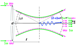
With the schematic view of QPS in Fig. 1, we briefly explain the essence of our method as follows. By using variables defined at QPS, the center of mass system (CMS) energy between a randomly selected photon pair is expressed as
| (1) |
where is the energy of incident photons and is half of the incident angle of the photon pair. Extremely low collision energies are realizable at QPS by focusing a laser field because small values of can be automatically introduced.
In order to overcome low scattering amplitudes of processes due to weak coupling, we first utilize the character of the integrated resonance effect by capturing within via prepared by a creation laser field. Secondly we let another laser field propagate into the optical axis common to the creation laser. This laser induces decay of resonance states into a specific energy-momentum space by the coherent nature of the inducing field. The scattering probability is thus proportionally increased by the number of photons in the inducing laser field DEptp ; TajimaHomma ; DEapb ; DEptep .
Energies of decayed photons are defined by the following energy conservation
| (2) |
where is an arbitrary number which satisfies . We re-define the energies of final state photons as following
| (3) |
where and are energies of signal photon and inducing photons, respectively.
In the case of the scalar field exchange, the relation of linear polarization states between initial and final state photons when the wave vectors are on the same reaction plane are expressed as follows:
| (4) |
where {1} and {2} are linear polarization states orthogonal to each other. In the pseudoscalar filed exchange, the polarization relation are expressed as
| (5) |
We emphasize that above relations are limited only to the theoretically ideal case where all four photons are on the same reaction plane within the treatment based on plane waves. In the focused QPS, however, we must accept independent rotations of the incident plane and the outgoing plane as illustrated in Fig. 13 with respect to an experimentally given linear polarization plane. This implies that even if we supply as the pure {1}-state by a polarizer at the moment of plane wave propagation in advance of focusing, mixing of {1} and {2} states for randomly selected incident photon pairs is unavoidable while lasers are focused. Therefore, the focused QPS with a fixed initial linear polarization plane has sensitivity to both scalar and pseudoscalar fields simultaneously. We discuss about this nature in detail in Appendix A.
The relation in Eq.(2) is similar to ”four-wave mixing” in matter corresponding to the third order non-linear quantum optical process in atoms FWM ; Yariv . Therefore, the observation of the four-wave mixing process in the vacuum may be interpreted as a replacement of the atomic nonlinear process by the exchange of unknown scalar or pseudoscalar fields. The observation of four-wave mixing in the vacuum is also used as a method for testing higher-order QED effect FWMqed1 ; FWMqed2 ; FWMqed3 ; FWMqed4 .
Photons produced via the atomic four-wave mixing process can be the main background source for this search. The first search for scalar fields at QPS hiroshima was performed with weak intensity lasers, thus, the effect of the four-wave mixing process in atoms was negligible. In this experiment, however, the four-wave mixing photons originating from the residual gas are anticipated due to much higher beam intensities. In this paper the method to obtain the exclusion limits in the search at QPS sensitive to both scalar and pseudoscalar fields is provided under the circumstance where a finite amount of background photons must be evaluated.
II The coupling-mass relation
The effective interaction Lagrangians coupling between two photons and / are expressed as
| (6) |
where has the dimension of energy and is the dimensionless constant. The yield of signal photons, , is expressed with experimental parameters relevant to lasers and optical elements as follows:
| (7) |
where the subscripts and indicate creation and inducing laser, respectively, is wavelength, is pulse duration, is focal length, is beam diameter, and are upper and lower values on determined by the spectrum width of , respectively, is mass of the exchanging field, is the numerical factor relevant to the integral of the weighted resonance function which is refined in Eq.(50) in Appendix B compared to in Ref.hiroshima , is the incident-plane-rotation factor described in Appendix A, is the polarization dependent axially asymmetric factor for outgoing photons DEptep , is the combinatorial factor originating from selecting a pair of photons among multimode frequency states and is the average numbers of photons in the coherent state. The detail of the formulation of the signal yield is summarized in Appendix of Ref.hiroshima . The coupling constant is expressed as
| (8) |
III Experimental setup
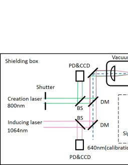
We explain the experimental setup to detect signals of four-wave mixing in the vacuum. The schematic view of the setup is shown in Fig. 2.
A Ti-Sapphire laser (wavelength 800 nm) and a Nd:YAG laser (wavelength 1064 nm) are used as the creation and the inducing lasers, respectively. To reduce the number of background photons emitted from the residual gas via four-wave mixing, the linear polarization states of the creation and inducing lasers are configured to linear polarization states {1} and {2}, respectively. The beam alignments of the lasers are monitored by CCD cameras (CCD) and the pulse energies of the creation and inducing lasers are measured by photo-diodes (PD). These beams are combined by a dichroic mirror (DM). The combined beams are guided into the vacuum chamber at the 20 mm beam diameter and focused with the convex lens at the focal length 200 mm.
The expected wavelength of the corresponding signal photon is evaluated from the following equation
| (9) |
A light source with the central wavelength of 640 nm is combined with the creation and inducing lasers by DM to evaluate the detection efficiency and to trace the trajectory of signal photons for the detector alignment.
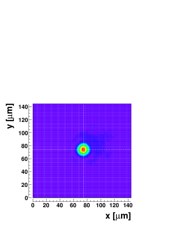
The agreement of the optical axes between the two lasers are adjusted at a precision of 2-3 m by monitoring individual beam profiles at the near side and the far side of the focal spot with the CCD camera. The beam profiles at the focal spot are shown in Fig. 3. The spot sizes of the creation and inducing lasers which are defined as 2 of the 2D Gauss functions fitting the beam profiles, are 21 m and 23 m, respectively. The creation laser overlaps with 87 % of the beam energy of the inducing laser at the focal spot. Thus, the effective beam energy of the inducing laser is evaluated by correcting the measured beam energy with this overlapping factor.

|
Signal photons generated within the focal volume travel along the common optical axis of the combined lasers. Signal photons are separated from the creation and inducing lasers by the prism and signal wave filters are placed to further eliminate the residual photons from the combined lasers. The polarization beam splitter (PBS) transmits {1}-polarized photons and reflects {2}-polarized photons. Incident photons are split between the shorter optical fiber Path{1} and the longer Path{2}. The incident photons to PBS are eventually observed by the common photo-device having relative time delay of 23 ns. We use a single-photon-countable photomultiplier tube (PMT) R7400-01 manufactured by HAMAMATSU as the photo-device.
The repetition rate of the creation laser is 1 kHz and that of the inducing laser is 10 Hz by synchronizing the trigger with the 1 kHz creation pulsing. The data acquisition trigger of 20 Hz is synchronized with the 1 kHz creation laser pulsing which includes pedestal triggers in order to provide four patterns of triggers. The time coincidence between creation and inducing pulses are performed by adjusting the relative injection timing between the two lasers so that the relative time maximizes the four-wave mixing yield in the air. The shutter is placed on the creation laser beam line and it repeats open and close every 5 sec. We acquire data with the four patterns of triggers, which are ”both of lasers are incident (S)”, ”only creation laser is incident (C)”, ”only inducing laser is incident (I)”, and ”neither of lasers are incident (P)”. The digital oscilloscope recorded waveform data from the PMT and two photo-diodes synchronized with the 20 Hz data acquisition trigger. The recorded waveform data from the PMT are sorted into four types of trigger patterns S, C, I and P. The four trigger patterns are classified by checking the charge correlations between the waveform data from the two photo-diodes for intensity monitoring.
IV Method of the waveform analysis
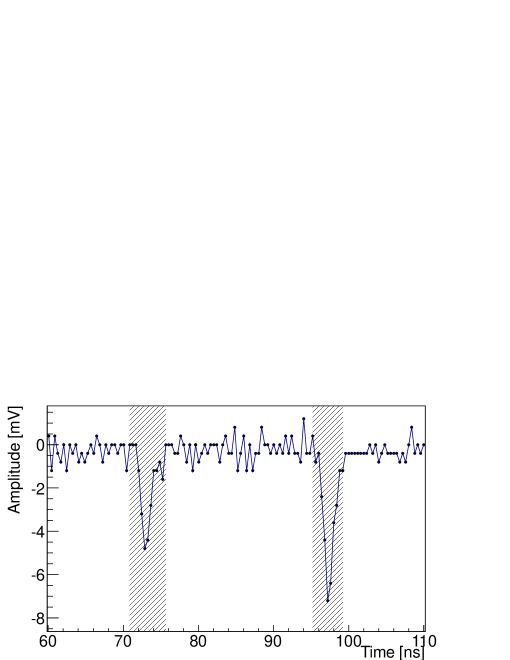
The observed photon counts are estimated by analyzing the waveform data from the PMT. The individual waveform consists of 500 sampling data points within a 200 ns time window. We search for negative peaks of which amplitude exceed a given threshold. We then calculate charge sums of the peak structures. Figure 4 shows a sample of waveform data where peak structures are identified. Charge sums of peak structures are evaluated in units of the single-photon equivalent charge, C.
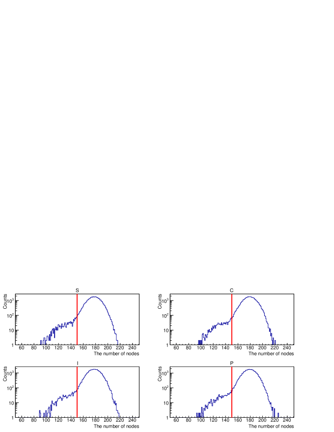
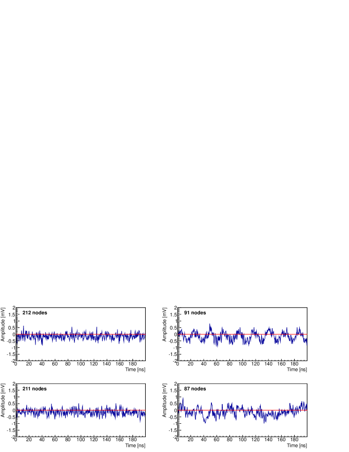
There are some accidental noisy events among recorded waveform data. In our analysis method, these noise structures could be misidentified as large photon-like peak structures. Therefore, it is necessary to remove such noisy events from analyzed waveform data before counting photon-like peaks. We can identify noisy events by analyzing the frequencies of waveforms. Noisy waveforms tend to have lower frequencies than those of normal waveforms. The frequencies are estimated by counting the number of nodes which is defined as the intersections between a waveform and the average line of amplitudes within the 200 ns time window. The distributions of the number of nodes for each trigger pattern are shown in Fig. 5. We regard a waveform of which the number of nodes is lower than 150 as a noisy event in all trigger patterns by confirming that the differences of the distributions among four trigger patterns are not prominent. The typical waveforms of noisy events and normal events identified by this method are shown in Fig. 6.
V Measurement of the four-wave mixing process in the residual gas
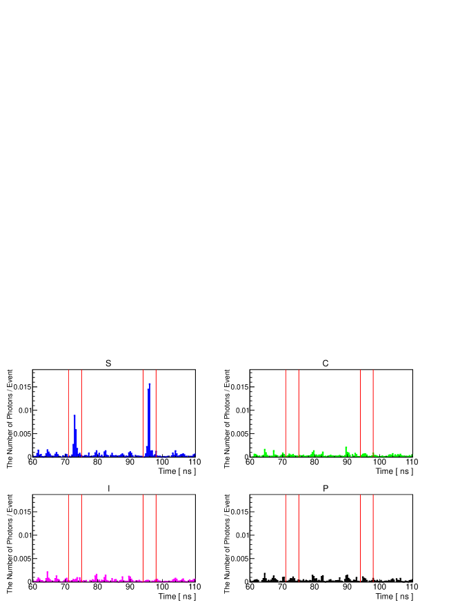
The background photons can be produced via the four-wave mixing process occurred in residual atoms in the vacuum chamber. To estimate the expected number of background photons, we measured the pressure dependence of the number of four-wave mixing photons in gas. Figure 7 shows arrival time distributions of observed photons in the air at Pa among four trigger patterns. Specific two peak structures appear only at S-pattern. These peak structures have approximately 23ns time interval, which agrees with the optical path-length difference between Path{1} and Path{2}. We count the number of photons within a time domain (71-75 ns) with {1}-polarized state and (94-98 ns) with {2}-polarized state.
The number of four-wave mixing signals are evaluated from the following equation. ( see Eqs.(18) and (19) in Ref.hiroshima )
| (10) |
where and denote the number of photon-like peaks in the signal domains and the number of events in trigger pattern , respectively.
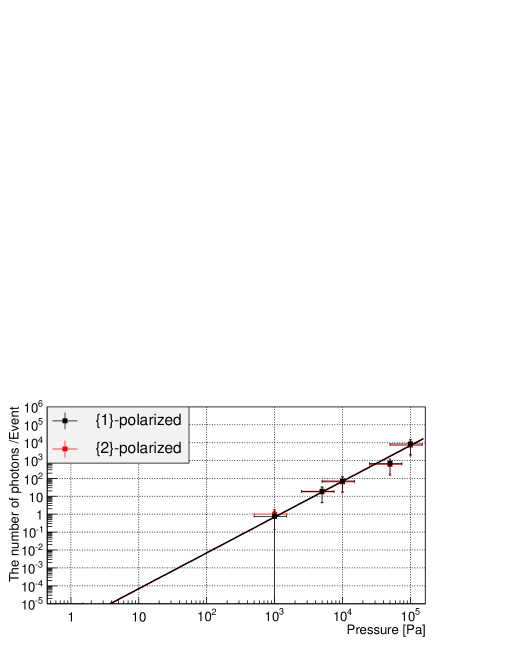
The pressure dependence of the number of four-wave mixing photons per S-trigger event are shown in Fig. 8. Data points are fit by the quadratic function of pressure. We extrapolate the number of four-wave mixing photons in the residual gas at Pa (an equivalent condition to the vacuum data we discuss later) from the fitting function. The efficiency-corrected number of {1}-polarized and {2}-polarized photons in residual gas and with the same shot statistics as the vacuum data are evaluated as follows:
| (11) |
We confirmed that the expected value of four-wave mixing photons from the residual gas are negligibly small in the vacuum data for a given total statistics.
VI Search for four-wave mixing signals in the vacuum
We acquired data at Pa for the search for the resonant states of and fields. Figure 9 shows the arrival time distributions of observed photon counts . Table 1 summarizes the numbers of observed photon-like signals evaluated in units of the single-photon equivalent charge with {1} and {2}-polarized states for each trigger pattern, respectively.
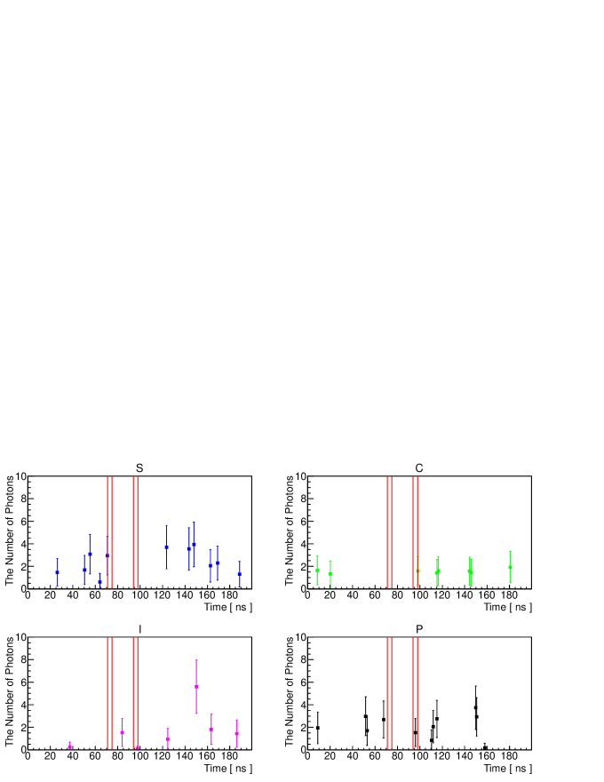
| Trigger | |||
|---|---|---|---|
| S | 0 | 0 | 46120 |
| C | 0 | 0 | 46203 |
| I | 0 | 0.07 | 46044 |
| P | 0 | 1.53 | 46169 |
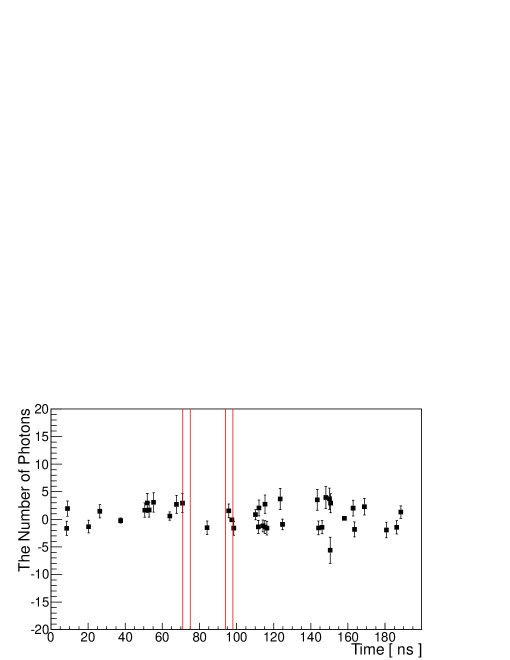
After performing subtractions between four patterns of histograms in Fig. 9 based on the relation in Eq.(10), we obtained the time distribution of as shown in Fig. 10. The number of signals with {1} and {2}-polarized states are, respectively, given as follows:
| (12) |
The systematic error I originates from the number of the photons out side of the two arrival time windows for {1} and {2}-polarized states. This was evaluated by calculating the root mean square of except in the and windows. The systematic error II originates from the dependence on the threshold values for the peak finding mV. The systematic error III is relevant to the ambiguities of the rejection of noisy events nodes.
VII The excluded coupling-mass limits for scalar and pseudoscalar fields
| parameters | values |
| center of wavelength of creation laser | 800 nm |
| relative line width of creation laser ( | |
| center of wavelength of inducing laser | 1064 nm |
| relative line width of inducing laser ( | |
| duration time of creation laser pulse per injection | 900 fs |
| duration time of inducing laser pulse per injection | 9 ns |
| creation laser energy per | 9.3 1.2 J |
| inducing laser energy per | 100 1 J |
| focal length | 200 mm |
| beam diameter of laser beams | 20 mm |
| upper mass range given by | 0.15 eV |
| 0.75 | |
| incident-plane-rotation factor | =19/32 |
| =1/2 | |
| axially asymmetric factor | =19.4 |
| =19.2 | |
| combinatorial factor in luminosity | 1/2 |
| single-photon detection efficiency | 1.4 0.1 % |
| efficiency of optical path from interaction point to path{1} | 0.5 0.1 % |
| efficiency of optical path from interaction point to path{2} | 0.9 0.2 % |
| 2.2 | |
| 4.4 |
There is no significant four-wave mixing signal in this search from the result in (12). We thus evaluate the exclusion regions on the coupling-mass relation as follows.
We estimate the upper limit on the sensitive mass range as
| (13) |
based on values summarized in Table 2, where in Fig. 1 varies from 0 to defined by a focal length and a beam diameter .
The number of efficiency-corrected {1}-polarized signal photons and that of {2}-polarized signal photons are evaluated from the following relations with the experimental parameters
| (14) |
where and are the attenuation ratios of the signal photons propagating from the interaction point through Path{1} and Path{2}, respectively.
These attenuation factors are composed of the transmittance of optical devices and the acceptance of signal paths with respect to the actual location of the PMT. They are inclusively evaluated by sampling the beam energies of the 640 nm calibration light at the focal point and the detection point, respectively, and taking the ratio between them. The matching of beam paths between the calibration light and four-wave mixing signals are ensured by adjusting the beam center of calibration light with respect to those of creation and inducing lasers at the near side and the far side of the focal spot, respectively. is the signal detection efficiency of the PMT mainly caused by the quantum efficiency of the device. is evaluated using a 532 nm pulse laser in advance of the search. We evaluate the absolute detection efficiency by splitting the 532 nm beam equally and taking the ratio between these energies. The one is measured by a calibrated beam energy meter and the other is measured by that PMT with neutral density filters with measured attenuation factors. We then corrected the difference of the quantum efficiencies between 532 nm and 641 nm lights by taking the relative quantum efficiencies provided by HAMAMATSU into account.
We then evaluate upper limits on the coupling-mass relation at a 95% confidence level on the basis that the fluctuation of the number of signal yields forms a Gaussian distribution. We define as the one standard deviation of . It is evaluated from the quadratic sum of statistical and systematic errors in Eq.(12) and 2.24 is the upper limit of when we obtain a 95% confidence level PDGstatistics . The upper limit of signal yields per shot (for the scalar field exchange) and (for the pseudoscalar field exchange) are evaluated as follows:
| (15) |
As we briefly mention in Introduction and in detail in Appendix A, even though we fix linear polarization planes for creation and inducing laser fields by the polarizers at the moment of plane wave propagation, mixing of {1} and {2}-polarization states is unavoidable in the focused QPS. By this effect, the focused system has sensitivity to both scalar and pseudoscalar fields simultaneously.
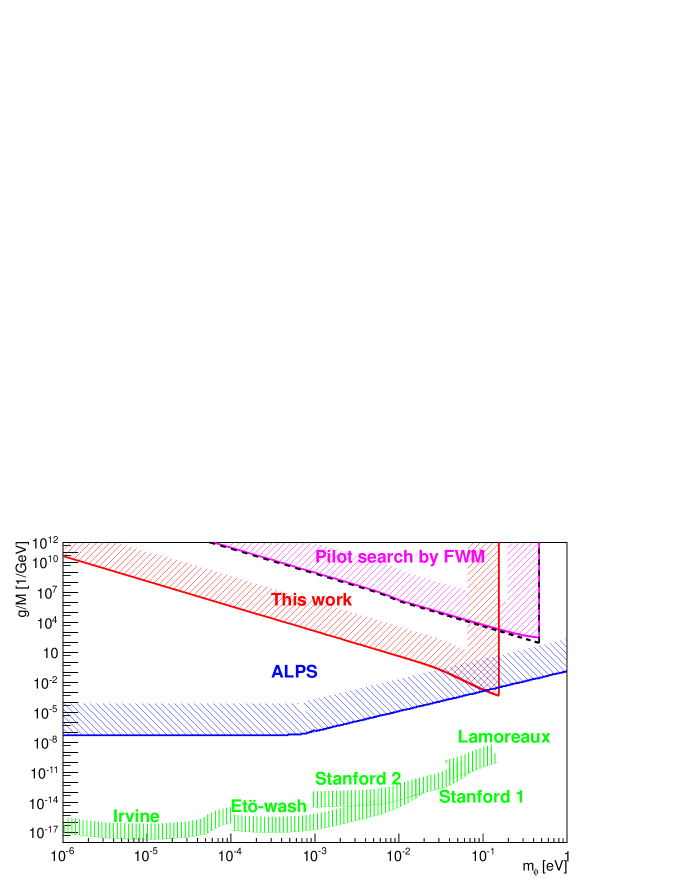
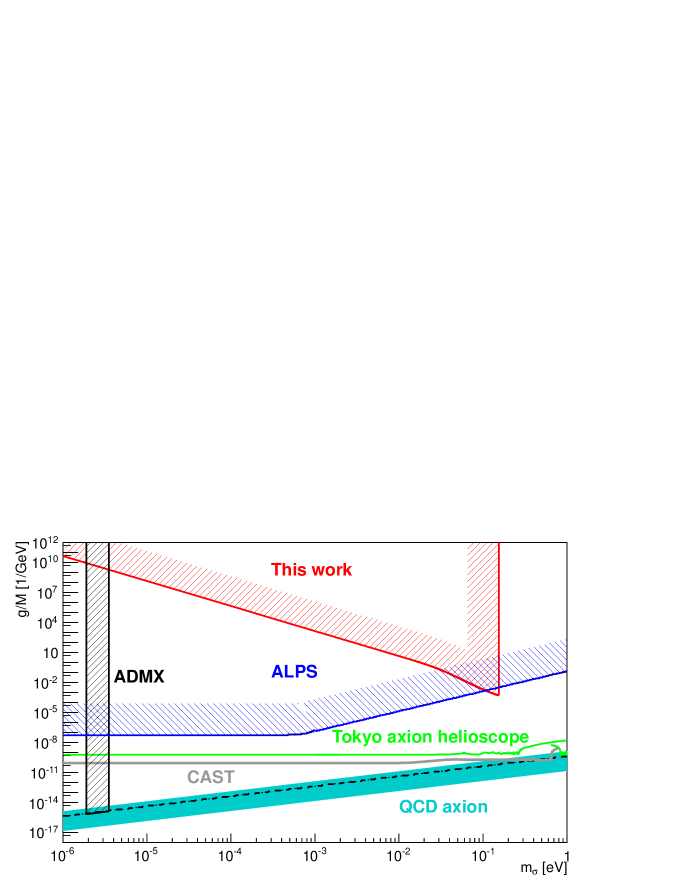
We obtain the coupling-mass relation from Eq.(8). The exclusion limits for scalar and pseudoscalar fields at a 95% confidence level are shown in Fig. 11 and Fig. 12 , respectively.
VIII Conclusions
A search for scalar and pseudoscalar fields via the four-wave mixing precess at QPS has been performed by focusing 10 J/0.9 ps pulse laser and 100 J/9 ns pulse lasers. The number of {1} and {2}-polarized signal-like photons are and , respectively. We confirmed that the expected number of four-wave mixing photons in the residual gas are negligibly small by measuring the pressure dependence. As a result, no significant four-wave mixing signal is observed in this experiment. We obtained the upper limits on the coupling-mass relation for scalar and pseudoscalar fields at a 95 confidence level, respectively. The most sensitive coupling limits for scalar search and for pseudoscalar search are obtained at eV.
Acknowledgments
We gratefully thank S. Tokita and Y. Miyasaka for operation and maintenance of laser systems. We appreciate Y. Inoue providing the data list of the sensitive curve for Tokyo axion helioscope.
K. Homma cordially thanks Y. Fujii for the detailed discussions and careful checks on the spin-dependence of the scattering probability. He expresses his gratitude to T. Tajima and G. Mourou for many aspects relevant to this subject. He also thank for the strong financial supports by the Grant-in-Aid for Scientific Research no.24654069, 25287060 and 26104709 from MEXT of Japan, Collaborative Research Program of Institute for Chemical Research, Kyoto University (grant No. 2012-6, No. 2013-56 and No. 2014-72) and the support by MATSUO FOUNDATION.
Appendix A: Evaluation of the incident-plane-rotation factor
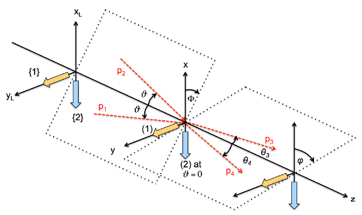
Figure 13 illustrates the relation between experimentally defined linear polarization directions {1} and {2} and those theoretically defined (1) and (2). It also depicts relations between and planes with respect to the plane where the theoretically allowed coupling of an exchanged field to the linear polarization states can be evaluated in the clearest way. In Ref.DEptep , we have assumed the incident photons and are both plane waves with different wave vectors on the same reaction plane which always ensures the clearest condition. In the general 3-dimensional incident case such as a focused Gaussian beam, however, a plane can rotate with respect to the plane, which results in a deviation from the theoretically clearest condition. We, therefore, introduce a weighted averaging factor over the clockwise rotation angle of the incident reaction plane with respect to the -axis as follows.
As we have discussed in ref.DEptep , the Lorentz invariant -channel scattering amplitude for Lagrangian defined in Eq.(6) have the following basic form
| (16) |
where with or , respectively, denotes a sequence of four-photon polarization states and is the mass of scalar or pseudoscalar field. With vectors defined below, the vertex factors for the scalar case (SC) are expressed as
| (17) |
and these for the pseudoscalar case (PS) are expressed as
| (18) |
We must first take into account the clockwise rotation angle of plane with respect to the given plane independent of the plane, because these two planes are not coplanar in QPS contrary to the situation where the coplanar condition of through is always satisfied in CMS. This implies that the simple summation factor on the azimuthal degree of freedom of solid angle cannot be applied to QPS, instead, the -dependent squared transition amplitude must be summed over the possible rotation from 0 to . We have already introduced this axially asymmetric factor with respect only to the incident reaction plane at in DEptep . This factor essentially depends only on the second vertex factors above, while the incident-plane-rotation factor is relevant only to the first vertex factors. We thus define the incident-plane-rotation factor as a weighted average with respect to at as follows
| (19) |
because experiments cannot fix the incident reaction plane and intensity of the creation laser field must be shared over possible incident reaction planes.
By requiring (1)={1} and (2)={2} at where theoretically clearest polarization relations can interface with the experimental condition, we describe the polarization vectors and momentum vectors for four photons with rotation angles and as follows:
| (20) |
| (21) |
We note here that we cannot rotate polarization vectors because the experiment must introduce fixed polarization vectors. This implies that the clear distinction between scalar and pseudoscalar couplings cannot be stated due to non-zero rotation angles because non-identical linear polarization planes between photon 1 and 2 or photon 3 and 4 are implicitly introduced.
Based on these vectors, we summarize relations between momenta and polarization vectors with photon labels as follows
| (22) |
| (23) |
for any pair , , and
| (24) |
and
| (25) |
where is required for massless photons.
We are now ready to estimate the factor included in the partially integrated cross section at Eq.(A24) in Ref.hiroshima . We evaluate the case of for the scalar exchange. From the first of Eq.(17), we obtain
| (26) | |||||
where the first of Eq.(25), Eq.(20), and are substituted. The last approximation is based on .
This yields the following averaging factor on the incident reaction plane
| (27) |
We also provide the case of for the pseudoscalar exchange as follows. Based on the first of Eq.(18), the first vertex factor with vector definitions above is expressed as
| (28) | |||||
This yields the following averaging factor on the incident reaction plane
| (29) |
Appendix B: Refinement of the weight factor
In Ref.DEptep ; hiroshima , we approximated as a constant for the mass region much smaller than that covered by as a conservative estimate. This is because we rather respected simplicity of the parametrization than accuracy. However, once we need to compare the sensitivity for the higher mass region with the other search methods, the validity of the approximation applicable only to the smaller mass region must be reconsidered. In the following, we first exactly repeat the relevant part of Ref.hiroshima and then refine as a function of sensitive mass regions by quoting necessary equations.
We first express the squared scattering amplitude for the case when a low-mass field is exchanged in the s-channel via a resonance state with the symbol to describe polarization combinations of initial and final states .
| (30) |
where with the resonance condition for a given mass and is expressed as
| (31) |
with the resonance decay rate of the low-mass field
| (32) |
The resonance condition is satisfied when the center-of-mass system (CMS) energy between incident two photons coincides with the given mass . At a focused geometry of an incident laser beam, however, cannot be uniquely specified due to the momentum uncertainty of incident waves. Although the incident laser energy has the intrinsic uncertainty, the momentum uncertainty or the angular uncertainty between a pair of incident photons dominates that of the incident energy. Therefore, we consider the case where only angles of incidence between randomly chosen pairs of photons are uncertain within for a given focusing parameter by fixing the incident energy. The treatment for the intrinsic energy uncertainty is explained in Appendix B later. We fix the laser energy at the optical wavelength
| (33) |
while the resonance condition depends on the incident angle uncertainty. This gives the expression for as a function of
| (34) |
where
| (35) |
We thus introduce the averaging process for the squared amplitude over the possible uncertainty on incident angles
| (36) |
where specified with a set of physical parameters and is expressed as a function of , and is the probability distribution function as a function of the uncertainty on within an incident pulse.
We review the expression for the electric field of the Gaussian laser propagating along the -direction in spatial coordinates Yariv as follows:
| (37) |
where electric field amplitude, , , is the minimum waist, which cannot be smaller than due to the diffraction limit, and other definitions are as follows:
| (38) |
| (39) |
| (40) |
| (41) |
With being an incident angle of a single photon in the Gaussian beam, the angular distribution can be approximated as
| (42) |
where the incident angle uncertainty in the Gaussian beam is introduced within the physical range as
| (43) |
with the wavelength of the creation laser , the beam diameter , the focal length , and the beam waist as illustrated in Fig.1. For a pair of photons 1, 2 each of which follows , the incident angle between them is defined as
| (44) |
With the variance , the pair angular distribution is then approximated as
| (45) |
where the coefficient 2 of the amplitude is caused by limiting to the range , and is taken into account because in Eq.(43) also corresponds to the upper limit by the focusing lens based on geometric optics. This distribution is consistent with the flat top distribution applied to Ref.DEapb ; DEptep except the coefficient.
We now re-express the average of the squared scattering amplitude as a function of in units of the width of the Breit-Wigner(BW) distribution by substituting Eq.(30) and (45) into Eq.(36) with Eq.(35)
| (46) |
where we introduce the following constant
| (47) |
with
| (48) |
In Eq.(47) the weight function is the positive and monotonic function within the integral range and the second term is the Breit-Wigner(BW) function with the width of unity. Note that is now explicitly proportional to but not . This gives the enhancement factor compared to the case where no resonance state is contained in the integral range controlled by experimentally. The integrated value of the pure BW function from to gives , while that from to gives . The difference is only a factor of two. The weight function of the kernel is almost unity for small , that is, when is small enough with a small mass and a weak coupling. Therefore, we will consider only the region of as a conservative estimate. By taking only this integral range, we can be released from trivial numerical modifications originating from and the behavior of at which are not essential due to the strong suppression by the Breit-Wigner weight.
We now refine in order to apply it more accurately even to the case for where, exactly speaking, the second approximation in Eq.(45) is not valid. In this case, by using the first of Eq.(45) with substitution of the relation between and expressed in Eq.(34), Eq.(48) is modified as follows
| (49) |
where the last approximation is based on with respect to the integral range in Eq.(47) for the conservative estimate. This is justified in the mass-coupling range we are interested in via the first relation in Eq.(31), for instance, for eV and GeV-1. By substituting Eq.(49) into Eq.(47), the conservative evaluation on over is expressed as
| (50) |
This factor is dependent of , equivalently dependent of mass, especially for larger close to while it is almost for smaller .
References
- (1) Y. Fujii and K. Maeda, The Scalar-Tensor Theory of Gravitation Cambridge Univ. Press (2003).
- (2) Y. Fujii and K. Homma, Prog. Theor. Phys 126, 531 (2011); Prog. Theor. Exp. Phys. 089203 (2014) [erratum].
- (3) K. Homma, Prog. Theor. Exp. Phys. 04D004 (2012); 089201 (2014) [erratum].
- (4) S. Weinberg, Phys. Rev. Lett 40, 223 (1978).
- (5) F. Wilczek, Phys. Rev. Lett 40, 271 (1978).
- (6) R. D. Peccei and H. R. Quinn, Phys. Rev. Lett 38, 1440 (1977)
- (7) M. P. Hertzberg, M. Tegmark, and F. Wilczek, Phys. Rev. D 78, 083507 (2008).
- (8) O. Wantz and E. P. S. Shellard, Phys. Rev. D 82, 123508 (2010).
- (9) S. Moriyama et al., Phys. Lett. B 434, 147 (1998).
- (10) Y. Inoue et al., Phys. Lett. B 536, 18 (2002).
- (11) Y. Inoue et al., Phys. Lett. B 668, 93 (2008).
- (12) K. Zioutas et al. (CAST Collaboration), Phys. Rev. Lett. 94, 121301 (2005).
- (13) S. Andriamonje et al. (CAST Collaboration), J. Cosmol. Astropart. Phys. 04, 010 (2007).
- (14) E. Arik et al. (CAST Collaboration), J. Cosmol. Astropart. Phys. 02, 008 (2009).
- (15) M. Arik et al. (CAST Collaboration), Phys. Rev. Lett. 107, 261302 (2011).
- (16) R. Cameron et al. (BRFT Collab.), Phys. Lett. D 57, 3873 (1993).
- (17) E. Zavattini et al. (PVLAS Collab.), Phys. Lett. D 77, 032006 (2008).
- (18) P. Pugnat et al. (OSQAR Collab.), Phys. Lett. D 78, 092003 (2008).
- (19) K. Ehret et al. (ALPS Collab.), Phys. Lett. B 689, 149 (2010).
- (20) S.J.Asztalos et al. (ADMX Collab.), Phys. Rev. D 69, 01101 (2004).
- (21) S.J.Asztalos et al. (ADMX Collab.), Phys. Rev. Lett. 104, 041301 (2010).
- (22) K. Homma, T. Hasebe, and K.Kume, Prog. Theor. Exp. Phys. 083C01 (2014).
- (23) T. Tajima and K. Homma, Int. J. Mod. Phys. A, vol. 27, No. 25, 1230027 (2012).
- (24) K. Homma, D. Habs, T. Tajima, Appl. Phys. B 106, 229 (2012).
- (25) S. A. J. Druet and J.-P. E. Taran, Prog. Quant. Electr. 7, 1 (1981).
- (26) Amnon Yariv, Optical Electronics in Modern Communications Oxford University Press (1997).
- (27) F. Moulin and D. Bernard, Opt. Commun. 164, 137 (1999).
- (28) E. Lundström et al., Phys. Rev. Lett. 96, 083602 (2006).
- (29) J. Lundin et al., Phys. Rev. A 74, 043821 (2006).
- (30) D. Bernard et al., Eur. Phys. J. D 10, 141 (2000).
- (31) See Eq.(36.56) in J. Beringer et al. (Particle Data Group), Phys. Rev. D 86, 010001 (2012).
- (32) Y. Su et al., Phys. Rev. D 50, 3614 (1994); 51, 3135 (1995) [erratum].
- (33) E. G. Adelberger et al., Phys. Rev. Lett. 98, 131104 (2007);
- (34) D. J. Kapner et al., Phys. Rev. Lett. 98, 021101 (2007).
- (35) J. Chiaverini et al., Phys. Rev. Lett. 90, 151101 (2003).
- (36) S. J. Smullin et al., Phys. Rev. D 72, 122001 (2005); 72, 129901 (2005) [erratum].
- (37) S. K. Lamoreaux, Phys. Rev. Lett. 78, 5 (1997); 81, 5475 (1998) [erratum].
- (38) J. E. Kim, Phys. Rev. Lett. 43, 103 (1979).
- (39) M. A. Shifman, A. I. Vainshtein and V. I. Zakharov, Nucl. Phys. B 166, 493 (1980).