Kinetic theory of a longitudinally expanding system of scalar particles
Abstract
A simple kinematical argument suggests that the classical approximation may be inadequate to describe the evolution of a system with an anisotropic particle distribution. In order to verify this quantitatively, we study the Boltzmann equation for a longitudinally expanding system of scalar particles interacting with a coupling, that mimics the kinematics of a heavy ion collision at very high energy. We consider only elastic scatterings, and we allow the formation of a Bose-Einstein condensate in overpopulated situations by solving the coupled equations for the particle distribution and the particle density in the zero mode. For generic CGC-like initial conditions with a large occupation number, the solutions of the full Boltzmann equation cease to display the classical attractor behavior sooner than expected; for moderate coupling, the solutions appear never to follow a classical attractor solution.
-
1.
McGill University, Department of Physics
3600 rue University, Montréal QC H3A 2T8, Canada -
2.
Institut de physique théorique, Université Paris Saclay
CEA, CNRS, F-91191 Gif-sur-Yvette, France -
3.
Institut für Kernphysik, Technische Universität Darmstadt
Schlossgartenstraße 2, D-64289 Darmstadt, Germany
1 Introduction and motivation
1.1 Context
A long standing problem in the theoretical study of heavy ion collisions is the time evolution of the pressure tensor and its isotropization [1, 2, 3, 4, 5, 6, 7, 8, 9, 10, 11, 12]. This question is closely related to the use of hydrodynamics in the modeling of heavy ion collisions. Although the complete isotropy of the pressure tensor is not necessary [13] for the validity of hydrodynamical descriptions, the ratio of longitudinal to transverse pressure, , should increase with time for a smooth matching between the pre-hydro model and hydrodynamics.
In most models with boost invariant initial conditions, the longitudinal pressure is negative immediately after the collision [14, 15] (in the Color Glass Condensate framework [16, 17, 18, 19, 20], this can be understood as a consequence of large longitudinal chromo-electric and chromo-magnetic fields). On timescales of the order of a few ( is the saturation momentum), the longitudinal pressure rises, and reaches a positive value of comparable magnitude to the transverse pressure. However, it is unclear whether the scatterings are strong enough to sustain this mild anisotropy, or whether the longitudinal expansion wins and causes the anisotropy to increase.
This regime may be addressed by various tools. Indeed, it corresponds to a period where the gluon occupation number is still large compared to 1, but small compared to the inverse coupling so that a quasi-particle picture may be valid. This means that the system could in principle be described either in terms of fields or in terms of particles. Since the occupation number is large, it is tempting to treat the system as purely classical. In a description in terms of fields, this amounts to considering classical solutions of the field equations of motion, averaged over a Gaussian ensemble of initial conditions whose variance is proportional to the initial occupation number. In a description in terms of particles, i.e. kinetic theory, this amounts to keeping in the collision integral of the Boltzmann equation only the terms that have the highest degree in the occupation number [21, 22, 23].
1.2 Classical attractor scenario
The field theory version of this classical approximation has been implemented recently [24] for scalar fields with longitudinal expansion, and it leads to a decrease of the ratio , like the power of the proper time. This behavior seems universal; it has been observed for a wide range of initial conditions, and both for Yang-Mills theory and scalar field theories with a point-like interaction (such as a interaction) [1, 2, 3]. Based on this observation, it was conjectured that the time evolution of can be decomposed in three stages, nicely summarized in Figure 3 of ref. [25] :
-
i.
A transient stage that depends on the details of the initial condition;
-
ii.
A universal scaling stage, called “classical attractor,” during which the dynamics is purely classical and the ratio decreases as ;
-
iii.
A final stage where the occupation number has become of order 1, and where quantum corrections are important. The isotropization of the pressure tensor may happen during this final stage.
1.3 Classical approximation in anisotropic systems
However, a possible difficulty with the classical approximation is that the occupation number cannot be large uniformly at all momenta, which may make this approximation unreliable since the dynamics integrates over all the momentum modes. In particular, this may be the case in anisotropic systems, as we shall explain now in a kinetic theory framework. Suppose for discussion that the particle distribution has become extremely anisotropic, with a narrow support in ,
| (1) |
This situation occurs in the pre-equilibrium stage of heavy ion collisions, that can be described at leading order by a rapidity independent classical color field. In a non expanding system111For a longitudinally expanding system, collisions will compete with the expansion, and the final outcome may depend on details of the scattering cross-section., we expect that scatterings will kick particles out of the transverse plane and restore the isotropy of the distribution.
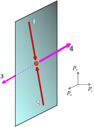
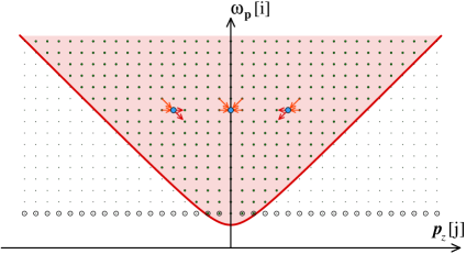
The Boltzmann equation that describes the evolution of should be able to capture this isotropization. If we track the momentum (see Figure 1), the Boltzmann equation can be sketched as follows:
| (2) | |||||
We have separated the purely classical terms (cubic in ) from the subleading terms that are quadratic in . The classical approximation amounts to dropping the quadratic terms. The usual justification of this approximation is to say that the cubic terms are much larger than the quadratic ones when . However, as we shall see now, this counting is too naive when the support of is anisotropic.
If and are in the transverse plane, then . Therefore, if we request that the particle 4 is produced outside of the transverse plane, then we have . Because of this, many pieces of the collision term (underlined in eq. (2)) are zero. In particular, all the classical terms vanish. The physical interpretation is clear: the terms correspond to stimulated emission, which cannot happen when both final particles lie in an empty region of phase space.
The only non-zero term is the one in , but one must go beyond the classical approximation in order to capture it. This is true no matter how large the distribution is inside its support, i.e. even if the classicality condition is satisfied there. Moreover, this argument can be trivially generalized to any scattering process in kinetic theory222The classical approximation of a collision term contains only terms of degree . Because of longitudinal momentum conservation, if one of the momenta points out of the transverse plane, then there must be at least one out-of-plane momentum. Therefore, of the distribution functions, at least one is zero.. Therefore, when the particle distribution is anisotropic, the classical approximation artificially suppresses out-of-plane scatterings at large angle, possibly resulting in wrong conclusions regarding isotropization.
Now let us relax the function assumption, and consider the case where the range of angles with large occupancy is finite but narrow. In particular, suppose that for momenta , the particles mostly reside with , where describes how anisotropic the momentum distribution is. We are interested in scattering processes which move particles out of this highly-occupied region. So consider a scattering process, where the final momentum lies outside this highly-occupied region, so is small. Within the classical approximation, Eq. (2) is dominated by the term. But for all three of these occupancies to be large, we need . Since , this ensures that , that is, the final state particle produced in a classical scattering must still have quite a small value. We will refer to these as classical scatterings. A scattering with and will always be suppressed by a small occupancy in the classical approximation, so these scatterings can be neglected classically, and only occur because of the quantum term in Eq. (2). We will call these quantum scatterings.
Now let us see whether scatterings with may still be important, even if the occupancies are large. First of all, while the integrand in Eq. (2) is small for quantum scatterings, the integration phase space is much larger for these processes. Specifically, since in all cases, and because of the momentum-conserving delta function, the phase space for “quantum” scatterings is larger than that for “classical” scatterings by a factor of . Therefore, even if the occupancy in the highly-occupied region is , order-1 of the scatterings are “quantum.” That is, order-1 of the scatterings involve quantum effects when the angle-averaged occupancy below is order 1. This argument may not apply in gauge theories, where the matrix element is strongly enhanced for small-angle processes, but it should be valid in a scalar theory where the matrix element is isotropic.
In addition, for many purposes, an individual scattering resulting in is much more important than a scattering resulting in . A particle’s contribution to the longitudinal pressure involves . The particle produced in a “quantum” scattering, with , contributes more to the longitudinal pressure than the classically-scattered particle, by a factor of . Therefore, in terms of generating longitudinal pressure, each “quantum” scattering contributes a more important effect, by a factor of . Combining this factor with the larger phase space for quantum scattering, we find that, for the purposes of understanding the longitudinal pressure, the classical approximation already starts to fail when , which is when the angle-averaged occupancy is .
This suggests that the classical approximation may lead to missing some contributions that are important for isotropization in theories where the cross-section is dominated by large-angle scatterings, such as a scalar theory. When the classical approximation is used in this theory, it has been observed in ref. [24] that the ratio decreases like at late times for a longitudinally expanding system (dotted curve in Figure 2). Given the above argument, the terms that are neglected in the classical approximation could alter this behavior sooner than one might naively expect, ending the growth of anisotropy and giving a ratio at late times. If the terms are truly negligible over some extended period of time, then the full Boltzmann equation should lead to the red curve in Figure 2,
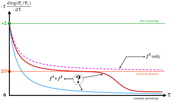
in which the system spends some time stuck into a classical attractor before eventually leaving it in order to isotropize (this red curve corresponds to the 3-stage scenario of Section 1.2). In contrast, if the terms are important from the start, one may get the behavior illustrated by the blue curve, where the power law does not play any particular role in the evolution of and a classical attractor would not exist.
1.4 Contents
In the rest of this paper, in order to assess quantitatively this issue, we solve the Boltzmann equation for an expanding system of scalar bosons with a interaction, both for the full collision kernel and its classical approximation. In Section 2, we discuss the Boltzmann equation for a longitudinally expanding system and prepare the stage for its numerical resolution. We describe our algorithm in Section 3, and the numerical results are exposed in Section 4. Section 5 is devoted to a summary and concluding remarks. Some more technical material and digressions are presented in appendices. In appendix A, we present results on the isotropization of the pressure tensor in a non-expanding system, that corroborate the fact that the terms play an essential role. In appendix B, we derive an analytical expression for the azimuthal integrals of the collision term. Additional details about our algorithm can be found in appendices C and D. In the appendix E, we present an alternate algorithm for solving the Boltzmann equation, based on the direct simulation Monte-Carlo (DSMC) method.
2 Boltzmann equation for expanding systems
2.1 Notation
In the following, we consider partially anisotropic particle distributions that have a residual axial symmetry around the axis,
| (3) |
(). For simplicity, we do not write explicitly the space and time dependence of . The function depends smoothly on momentum, except possibly at if there is a Bose-Einstein condensate (see Section 2.4). We also assume that is even in the longitudinal momentum
| (4) |
The Lorentz covariant form of the Boltzmann equation reads
| (5) |
where is the collision term (see the subsection 2.3). This form of the equation can then be specialized to any system of coordinates. We will focus on the collision term which arises at lowest order in the coupling, which for theory is elastic scattering.
For a system that expands in a boost invariant way in the longitudinal direction, the most appropriate system of coordinates is for the space-time coordinate and for the momentum of the particle, which are related to the usual Cartesian coordinates and momenta by
| (6) |
The assumed boost invariance of the problem implies that the distribution does not depend separately on and , but only on the difference . Therefore, it is sufficient to derive the equation for the distribution at mid-rapidity, . For simplicity, we will further assume that the distribution is independent of the transverse position.
2.2 Free streaming term
In the system of coordinates defined in eqs. (6), the left-hand side of the Boltzmann equation can be rewritten as
| (7) |
where we have defined
| (8) |
In a boost invariant system, depends on and only via the difference and it is sufficient to consider only the distribution at mid-rapidity, , for which we have
| (9) |
This formula implicitly assumes that the distribution is given in terms of the transverse momentum and the rapidity . Energy and momentum conservation will take a simpler form if we express it in terms of the energy and longitudinal momentum , instead of and . Since and , one gets333The more familiar form is obtained when one expresses in terms of and .
| (10) |
2.3 Collision term
If we consider only scatterings, the right-hand side of the Boltzmann equation contains integrals over the on-shell phase spaces of three particles. This 9-dimensional integral can be reduced to a 5-dimensional integral by using energy and momentum conservation. A further simplification results from our assumption that the distribution is invariant under rotations around the axis. The Boltzmann equation reads
| (11) |
with
| (12) |
In this equation, denotes the integration over the invariant phase-space
| (13) |
and is the factor that contains the particle distribution444The subscript “nc” means “no condensate”. In the next subsection, we will generalize this equation to the case where Bose-Einstein condensation can happen.,
| (14) |
(We use the abbreviation .)
The invariance under rotation around the axis can be used in order to perform analytically all the integrals over azimuthal angles (we use the same procedure as in the case of an rotational invariance, see refs. [26, 27]). In order to achieve this, let us first write
| (15) |
By combining this with the integrations over the transverse momenta, we get
| (16) |
The integral over depends only on the transverse momenta , but not on the distribution function . It can therefore be calculated once for all. In the appendix B, we obtain an explicit formula for this integral in terms of the Legendre elliptic function. Defining
| (17) |
we obtain
| (18) |
where555In the appendix B, we present a simple and fast algorithm for evaluating .
| (19) |
In terms of this integral, the collision term reads
| (20) |
For the sake of brevity, we have not written explicitly the boundaries of the integration range on . They are given by
| (21) |
Eq (20) reduces to a 4-dimensional integral after taking into account the two delta functions, which is doable numerically. Assuming that we encode the momenta with there is no need to perform any interpolation when using the delta functions to eliminate two of the integration variables, which is useful for fulfilling with high accuracy the conservation of energy and particle number. After this reduction that eliminates the variables and , eq. (20) reduces to
| (22) |
At each time step, must be calculated for each value of and . Therefore, if we discretize the variables and with and lattice points respectively, the computational cost for each time step scales as .
In the numerical implementation, the allowed energy and momentum ranges must be bounded. We will denote the maximum allowed energy as and the maximum allowed longitudinal momentum as , so that
| (23) |
The integration domain for and is the bounded domain shown in Figure 3.
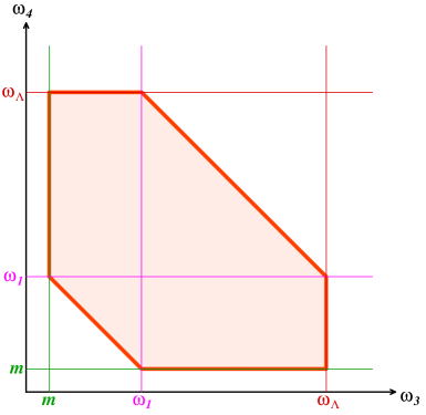
Likewise, if we assume that (since is even in ), the integration domain for and is the domain shown in Figure 4.
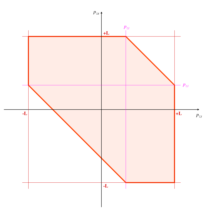
The peculiar shape of these domains comes from the fact that and extracted from the delta functions must themselves have values which lie within the bounds (23). The variable can be positive or negative, and although is even in , we must integrate over both and inside the collision term, because of the asymmetric shape of the integration domain. Note that there is also an extra constraint (not represented on these diagrams because it relates and ) that must be satisfied,
| (24) |
for the transverse momentum to be defined.
2.4 Bose-Einstein condensation
If only elastic collisions are taken into account, a Bose-Einstein condensate (BEC) may appear in the system if the initial condition is overpopulated [4, 28, 29, 30, 31]. When this happens, the particle distribution has a singularity at zero momentum, that we can represent by666Our convention for the integral of a delta function over the positive real semi-axis is so that the integral of the second term with the measure gives .
| (25) |
After this redefinition, describes the smooth part of the occupation number and is the particle density in the condensate. The Boltzmann equation (11) needs to be revised to account for . Indeed, one can now have particle-condensate interactions. One can easily check that the processes cannot involve more than one particle from the condensate. The modified Boltzmann equation thus reads
| (26) |
where is the contribution from collisions between the particle of momentum that we are tracking and a particle from the condensate,
| (27) |
while stands for a collision between the particle that we are tracking and another particle of momentum to give a final state with a particle in the condensate and a particle of momentum ,
| (28) |
This term should be doubled, to account for the fact that the condensate particle can be the particle or the particle . Following the same procedure777Here one can directly use the formula (73) for the integral of three Bessel functions. as in Section 2.3, we find
| (29) |
where is the area of the triangle of edges :
| (30) |
Note that in these collision terms, the 2-dimensional integration domains of Figures 3 and 4 collapse to 1-dimensional domains (see the appendix C).
The equation for the evolution of the particle density in the condensate can be obtained from eq. (22), by replacing the particle that we are tracking with the singular part of eq. (25), and then integrating over . By doing so we obtain the following equation for the condensate
| (31) |
where the integration domains are those of Figures 3 and 4 (with and ).
2.5 Conservation laws
The Boltzmann equation fulfills several conservation laws, that play an important role in determining the form of the equilibrium particle distribution and also in assessing the accuracy of algorithms employed for solving the equation numerically. Each collision conserves energy and momentum. In addition, since we are only considering elastic scatterings in this paper, the collisions also conserve the number of particles.
The particle density is given by
| (32) |
Note that this is a density of particles per unit of rapidity . Since a given interval of corresponds to a volume that expands linearly with the proper time , the conservation of the total number of particles implies that
| (33) |
Likewise, the components of the energy-momentum tensor are given by
| (34) |
(.) In a longitudinally expanding system, the conservation of energy and momentum, , becomes
| (35) |
where is the energy density and is the longitudinal pressure.
The fact that the solutions of the Boltzmann equation satisfy the conservation equations (33) and (35) is a consequence of the delta function and of the symmetries of the collision term under various exchanges of the particles . Namely, the integrand in the collision term is symmetric under the exchange of the initial state or final state particles :
| (36) |
and antisymmetric if we swap the initial and final states:
| (37) |
Therefore, any approximation scheme used in a numerical algorithm should aim at satisfying these properties with high accuracy. The easiest way to implement the delta functions without loss of accuracy is to use a lattice with a constant spacing in the variables and . By doing this, one is guaranteed that the values of and obtained by solving the constraints provided by the delta functions are also points on this grid. In addition, the quadrature formulas used for approximating the integrals in the collision term should lead to
| (38) |
which are consequences of the symmetries (36) and (37). In other words, even if these symmetries are manifest in the collision kernel, one should be careful not to violate them with an improper choice of the quadrature weights. As we will see, our numerical scheme respects these symmetries, so that the conservation laws can be satisfied up to machine precision.
It is also important to realize the role played in the conservation laws by the terms
| (39) |
that appear on the left-hand side of the Boltzmann equation. For instance, these terms provide the term in eq. (35), since we have
| (40) |
However, this identity relies on a cancellation between the boundary terms that result from the integration by parts on and . This must be kept in mind when discretizing the free streaming part of the Boltzmann equation, in order to avoid introducing violations of the conservation laws through these boundary terms.
2.6 Classical approximation
A central question in this paper is the interplay between the classical approximation and isotropization. Each computation will therefore be performed twice:
- i.
- ii.
As will become clear in the description of our algorithm in the next section, we use fixed cutoffs on the energy and on the longitudinal momentum . These cutoffs are not exactly the same as in the implementation of the classical approximation in classical lattice field theory, where one uses fixed cutoffs on the transverse momentum and on the Fourier conjugate of the rapidity. Indeed, , so that a fixed cutoff on roughly corresponds to a cutoff on that grows linearly with time. Fortunately, we do not expect physical effects from these cutoffs if they are taken high enough, since the occupancy typically falls off exponentially at large energy and momentum.
Note that there is a variant of the classical approximation defined in (41), in which each distribution function is replaced by . It is well known that this Ansatz provides the correct quadratic terms [21, 22], accompanied by some spurious terms that are linear in the distribution function. This variant is known to suffer from a severe ultraviolet cutoff dependence, when the cutoff becomes large compared to the physical scales [32] (this property is closely related to the non-renormalizability of a variant of the classical approximation in quantum field theory, where one includes the zero point vacuum fluctuations [33]). For this reason, our algorithm for the Boltzmann equation in a longitudinally expanding system cannot be employed to study this alternate classical approximation, because of its fixed cutoff in , while the physical s decrease with time due to the expansion. In appendix A, where we consider the question of isotropization in a non-expanding system, we have also included this variant of the classical approximation (labeled “CSA” in Figures 15 and 16) to the comparison with the full calculation, and it appears that the quadratic terms in included within this variant considerably improve the agreement with the full Boltzmann equation regarding isotropization.
3 Algorithm
3.1 Discretization
We adopt the following discretization for the longitudinal momentum and the energy:
-
The longitudinal momentum is taken in the range , which we discretize into points (including the endpoints ). The longitudinal step and the discrete values (with ) are given by
(42) -
The energy is taken in the range , which is discretized in points. The step and the discrete values (with ) are given by
(43) -
The transverse momentum is then defined as
(44) with and . If the inequality is not satisfied, then the pair is excluded from the lattice.
-
The particle distribution is encoded as a function of and . In addition, the assumed parity of in translates into
(45)
The motivation for this choice is that, with uniformly spaced discrete energy values, a scattering from a pair of lattice points to a pair of lattice points will exactly represent energy conservation. Further, an integral over all momenta can be represented as a sum over lattice positions; no sampling or Monte-Carlo integration errors ever arise, only errors from the discretization procedure itself.
3.2 Collision term
Let us now present an algorithm that preserves all the symmetries of the collision kernel. This algorithm is a simple extension of the one used in ref. [32] (appendix B.2). For simplicity, we can assume that , since the particle distribution is even in . The integrals over and in the collision kernel are approximated by two 1-dimensional quadrature formulas. For the integral of a function , we use
| (46) |
In our implementation, we have chosen the weights as follows888Our choice of the quadrature weight assumes that also includes the particles in the energy bin .
| (47) |
Similarly, for integrations over the longitudinal momentum we use
| (48) |
with the following weights
| (49) |
If we denote the integers corresponding to the momentum , the expression (20) for the collision kernel in the absence of condensate can thus be approximated by
| (50) |
In these sums, one should discard any term for which one of the pairs does not comply with the inequality (44). Eqs. (38) have been checked to hold with machine accuracy with this scheme. Similar formulas can be written for the terms that describe collisions involving a particle from the condensate, and they are given in appendix C.
3.3 Free streaming term
In the absence of collisions (e.g., in the limit ), the Boltzmann equation describes free streaming, a regime in which each particle moves on a straight line with a constant momentum. In the system of coordinates , we are describing a slice in the rapidity variable . This slice is progressively depleted of its particles with a non-zero , since they eventually escape, and the support of the particle distribution in therefore shrinks linearly with time.
On our lattice representing discrete values of and , the derivatives with respect to and that appear on the left-hand side of the Boltzmann equation represent the fact that each particle systematically loses , and therefore energy . The trajectory of a particle in space, shown in Fig. 5, will be inward and downward. Discretizing the allowed values, this can be viewed as the particles hopping inward and downward. For instance, the particle number on the site will move towards the sites999This choice is not unique. For instance, one could instead consider hops to or , which would correspond to a different discretization of the derivatives and . We choose this discretization because the change is always larger than the change, and because the point almost always exists, while along the kinematic boundary the point generally does not. and . Meanwhile, particle number living on the site or will flow onto the site . In contrast, a particle on the site (i.e. ) can hop to or , while a particle located at or can jump to . Once a particle reaches the line , it does not move from there. These moves are illustrated in Figure 5.
Since , it is sufficient to consider . Let us denote the number density of particles at site as
| (51) |
The most general form for a discrete version of the collisionless Boltzmann equation can be written as101010The special case is written explicitly in the eq. (92) of the appendix D.
| (52) |
where are coefficients that will be adjusted in order to satisfy all the conservation laws111111We can disregard the condensate in this subsection. Indeed, since the particles in the condensate have zero momentum, they play no role in free streaming, which simply causes the condensate number density to decay as ..
The non-condensed contribution to the particle density reads
| (53) |
Similarly, we can write its contribution to the energy density and longitudinal pressure as follows
| (54) | |||||
| (55) |
In order to fully determine the unknown coefficients, we also need to consider the first moment of the distribution of longitudinal momenta,
| (56) |
In the appendix D, we show that must have the following form121212A limitation of our scheme is that it works only if the points are not allowed by the condition , i.e. if This can be fulfilled by choosing appropriately the lattice parameters (these points have been surrounded by a circle in Figure 5 – in the example of this figure, the above inequality is not satisfied). All the numerical results shown in this paper have been obtained with a lattice setup that satisfies this condition.:
| (57) |
Starting from (52) and replacing the local particle density by (51), we obtain the following discretization (for ) for the free streaming equation
| (58) | |||||
In the particular case , this equation reads
| (59) |
One can also rewrite eq. (58) as
| (60) |
For the internal points, where all the weights and are equal to one, this becomes
| (61) | |||||
which indeed reproduces the left-hand side of the Boltzmann equation (26) in the continuum limit.
4 Numerical results
4.1 CGC-like initial condition
We now solve the coupled equations (26) and (31) with the algorithm described in the previous section. We have used a moderately anisotropic initial condition that mimics the gluon distribution in the Color Glass Condensate at a proper time . It is characterized by a single momentum scale , below which most of the particles lie. The scale also sets the unit for all the other dimensionful quantities. To be more specific, our initial distribution at the initial time is:
| (62) |
with a large occupation below , . According to the standard argument, such a large value of should ensure that the classicality condition is well satisfied, and that the cubic terms alone lead to good approximation of the full solution. We choose a coupling constant131313Although this may seem to be a large value, it corresponds to a rather small scattering rate, because of the prefactor in front of the collision integral. Another point of view on this value is to recall that the screening mass in a scalar theory at temperature is , while in Yang-Mills theory with 3 colors it is . Thus, if the two theories were compared at equal screening masses, one would have . Alternatively, if we compare the two theories at the same shear viscosity [34, 35, 36] to entropy density ratio, the scalar and gauge couplings should be related by . A coupling in the scalar theory would correspond to a very small strong coupling constant (conversely, would correspond to choosing in the scalar theory). Note that if is the coupling at the scale , then the Landau pole of the theory is at the scale – sufficiently above to justify a perturbative treatment. . The particle density in the condensate is initially , and the mass is taken to be . Finally, the cutoffs are and , while . The initial anisotropy was moderate, controlled by the parameters and .
In Figure 6, we show the time evolution of and in the unapproximated and in the classical schemes. should be strictly constant141414Our discretization of the momentum integrals ensures exact conservation equations only if the time derivatives are evaluated exactly. The numerical resolution of the Boltzmann equation therefore also introduces an error that depends on the timestep and on the details of the scheme used for the time evolution. With our implementation, the quantity is conserved with machine precision, and the expected conservation law is exactly recovered in the limit . in both cases, since the conservation of particle number is not affected by the classical approximation (thus, this quantity is just used to monitor how well this conservation law is satisfied in the numerical implementation).
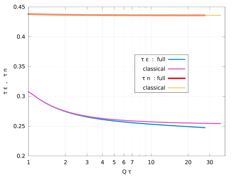
A small difference between the two schemes is visible in the energy density. Given the conservation equation (35), this also indicates that the two schemes lead to different longitudinal pressures. Since the unapproximated scheme leads to a faster decrease of the energy density than the classical scheme, it must have a larger longitudinal pressure. This will be discussed in greater detail later in this section.
4.2 Bose-Einstein condensation
The initial condition that we have chosen corresponds to a large overpopulation, since . If the system were not expanding, we would expect the formation of a Bose-Einstein condensate. Figure 7 shows the particle density in the zero mode in the unapproximated and classical schemes.
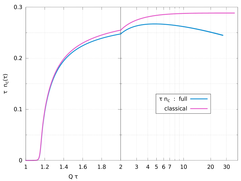
The onset of Bose-Einstein condensation is nearly identical in the two schemes, and a moderate difference develops at later times, that reaches about 20% at . The rather small difference between the two schemes for this quantity can be understood from the fact that the evolution of the condensate is governed by the region of small momenta, where the particle distribution is very large. We also see here a trend already observed in the isotropic case in ref. [32]: the classical approximation leads to more condensation than the unapproximated collision term. In fact, when the ultraviolet cutoff is large compared to the physical momentum scales, most of the particles tend to aggregate in a condensate in the classical approximation.
We mention in passing that our algorithm is not particularly well suited for a detailed study of the infrared region. The fixed energy spacing of our discretization lacks resolution in the IR, and our treatment of the mass as fixed, rather than a self-consistently determined thermal mass, is another limitation. On the other hand, the infrared has the highest occupancies, so classical methods are most reliable there. Therefore, lattice classical field simulations are much better suited for studying the infrared region. In particular our method is too crude to reveal the interesting scaling regimes found for instance in Ref. [2]. For this reason we will concentrate on quantities which are controlled by the higher-energy excitations, such as the components of the pressure.
4.3 Pressure anisotropy
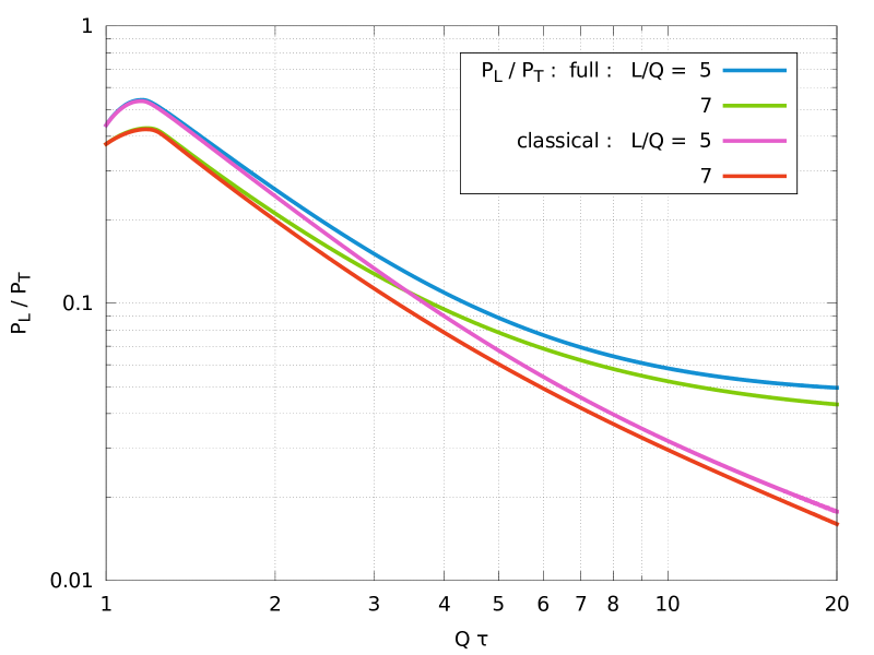
More important differences between the two schemes can be seen in the behavior of the longitudinal pressure. In Figure 8, we display the time evolution of the ratio . The beginning of the evolution is similar in the two schemes, with a brief initial increase of this ratio due to scatterings. Rapidly, the expansion of the system takes over and makes the ratio decrease, but at a pace slower than free streaming (indicated by a band falling like ). The two schemes start behaving differently around , with the classical approximation leading to a faster decrease of the ratio , approximately like . In contrast, the unapproximated collision term seems to lead to a constant ratio at large times.
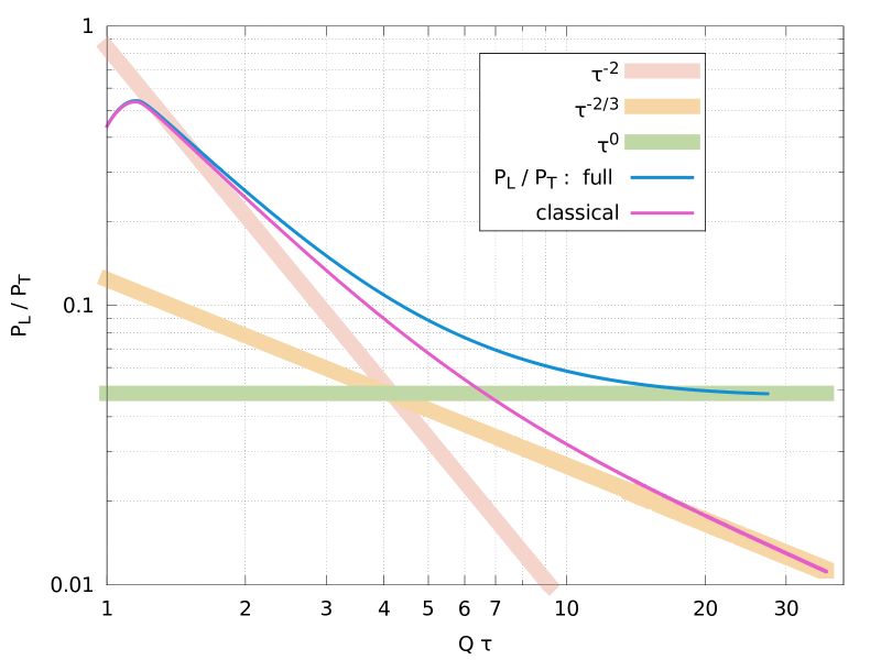
In Figure 9, we display the quantity as a function of time. If we parameterize
| (63) |
and if the exponent is slowly varying, then gives the instantaneous value of this exponent. This figure is to be compared with Figure 2, where several scenarios for the behavior of this exponent have been presented.
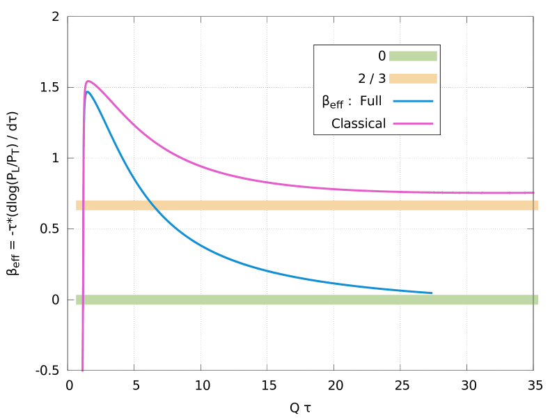
On this plot, we see that this exponent behaves quite differently in the two schemes, the asymptotic exponent being close to in the classical approximation, while it is zero with the unapproximated collision term. Moreover, the exponent does not appear to play any particular role when one uses the full collision term, since does not spend any time at this value in this case, despite the large occupation number in this simulation. Therefore, the classical attractor scenario represented by the red curve in Figure 2 is not realized for this combination of initial condition and coupling. This computation also indicates that the condition , that was regarded as a criterion for classicality, should be used with caution. In this example, it does not guarantee that the classical approximation describes correctly the evolution of the system. This condition is imprecise because is in fact a function of momentum, and may not be true over all the regions of phase-space that dominate the collision integral.
Note that if the ratio is approximately constant,
| (64) |
(as is the case in the full calculation at large times) then we have
| (65) |
and the overpopulation measure behaves as follows:
| (66) |
For an isotropic system, and is a constant, and the Bose-Einstein condensate would survive forever (in our kinetic approximation where inelastic processes are not included). If the system remains anisotropic at large times, we have and decreases. Therefore, one expects that, if a condensate forms, it has a finite lifetime because the overpopulation condition will not be satisfied beyond a certain time. The final outcome should therefore be the disappearance of the condensate. The beginning of this process is visible in Figure 7 in the case of the unapproximated collision term.
We have also investigated the sensitivity of our algorithm to the ultraviolet cutoff on the longitudinal momentum. This cutoff may indeed have an important influence on the result since the typical of the particles in the system evolves with time due to the expansion. In Figure 10, we compare the results for and . We observe that the difference between the two cutoffs is essentially the one inherited from the initial condition, i.e. the fact that the tail of the Gaussian in eq. (62) extends further when we increase the cutoff.
The qualitative differences between the classical and full results are independent of the value chosen for this cutoff.
In Figure 11, we vary the coupling constant in order to see how the asymptotic behavior of the full solution is affected by the strength of the interactions.
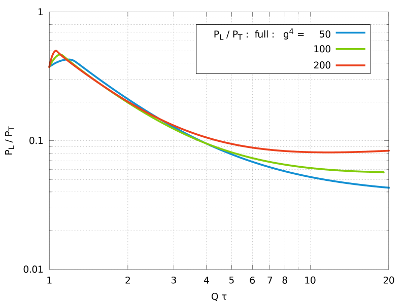
For the three values of the coupling, the ratio reaches a minimum, whose value increases with the coupling. For the largest of the couplings we have considered (, i.e. ), this ratio even shows a slight tendency to increase after a time of order .
4.4 More results using the DSMC algorithm
The deterministic algorithm we have used so far provides a direct resolution of the Boltzmann equation, but requires at each timestep the very time consuming computation of the collision integral. Moreover, it has a rather unfavorable scaling with the number of lattice points used in order to discretize momentum space. For this reason, we have also implemented a stochastic algorithm, the “direct simulation Monte-Carlo” (DSMC, described in the appendix E), where the distribution is replaced by a large ensemble of simulated particles. By construction, energy, momentum and particle number are exactly conserved with this algorithm (provided the kinematics of the collisions is treated exactly). Its sources of errors are the limited statistics, and the reconstruction of the particle distribution from the simulated particles (this step requires a discretization of momentum space, which leads to some additional errors).
Before showing more results using this algorithm, we have first used it with the same initial condition already used with the deterministic method, in order to compare the two approaches. The outcome of this comparison is shown in Figure 12, and indicates a good agreement between the two methods.
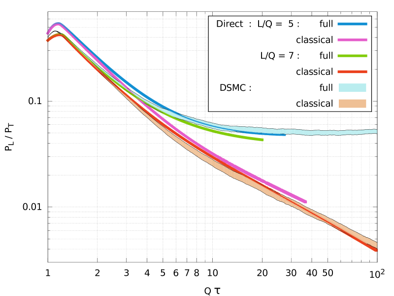
The differences, in the 10 % to 20 % range, can be attributed to the fact that the deterministic method simply disregards the particles with momenta higher than the lattice cutoffs. In contrast, in the DSMC method, there is no limit on the momenta of the simulated particles, and a discretization of momentum space is only used when reconstructing the distribution from the ensemble of particles.
We have then used the DSMC algorithm in order to study the time evolution of the pressure ratio in two situations:
First, we fix the value of the coupling constant at , and we vary the prefactor in the initial condition given by eq. (62). The parameters and that control the initial anisotropy of this distribution are also held fixed, as well as the initial time .
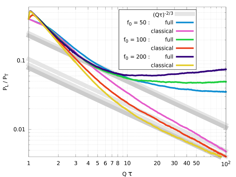
Although one may naively expect the agreement between the full and classical results to improve when is increased, Figure 13 shows that this is not the case. For the three values of considered in this computation, the classical approximation departs from the full result at roughly the same early time (or even a little earlier for the largest ). No matter how large , the ratio becomes roughly constant at late times –or even slightly increases– in the full calculation, and decreases like in the classical approximation.
Next, in a second series of computations, we have varied simultaneously the coupling constant and the initial occupation number in such a way that remains constant, . The parameters and controlling the initial anisotropy are the same as before.
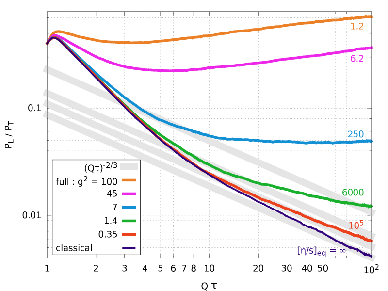
The resulting evolution of the ratio is shown in the figure 14. In the classical approximation, the pressure ratio falls like , as already observed earlier. Note that we have represented only one classical curve, common to all the values of . Indeed, since the collision term in this approximation is homogeneous in , one can factor out a prefactor and combine it with the of the squared matrix element, so that the classical dynamics is always the same if is held fixed. In contrast, the full dynamics does not posses this invariance, but appears to converge towards the classical result when . At finite coupling, the agreement between the full and classical results is good only over a finite time window, that shrinks as increases. At moderate values of the coupling such as (corresponding to , see Footnote 13), the unapproximated evolution departs from the classical one at a rather early point in time, and the exponent does not play any particular role in the evolution of . Two larger values of the coupling ( and ) are also shown on this plot, but one should not take the corresponding results seriously. Indeed, scalar theory with such a large coupling is not really self-consistent, because the coupling runs very fast and the Landau pole is only a factor of 5 to 20 away.
5 Summary and conclusions
This paper started with the qualitative observation that large-angle out-of-plane scatterings are artificially suppressed by the classical approximation of the collision term in the Boltzmann equation with scatterings, when the particle distribution is anisotropic, as is generically the case for a system subject to a fast longitudinal expansion. This kinematics is for instance realized in the early stages of heavy ion collisions.
In order to quantify this effect, we have considered a longitudinally expanding system of real scalar fields with a interaction in kinetic theory, and we have solved numerically the Boltzmann equation with elastic scatterings in two situations: (a) with the full collision term, and (b) in the classical approximation where one keeps only the terms that are cubic in the particle distribution.
This numerical resolution has been performed with two different algorithms. The first one is a direct deterministic algorithm, in which one discretizes momentum space on a lattice in order to compute the collision integrals by numerical quadratures (by assuming a residual rotation invariance around the axis, we could perform the azimuthal integrals analytically). The second method we have considered is a variant of the direct simulation Monte-Carlo (DSMC), in which the distribution is sampled by a large number of “simulated” particles.
The outcome of these computations is that the classical approximation is not always guaranteed to be good –even at a qualitative level– in situations where the occupation number is large. At moderate values of the coupling constant, the classical attractor scenario cartooned in Figure 2 is never observed, and the pressure ratio becomes constant at late times or even increases without showing any sign of a behavior in the full calculation (while a behavior is indeed seen at late times in the classical approximation). Increasing the occupation number at fixed coupling does not make the classical approximation any better. The classical behavior, with behavior in the longitudinal pressure, does emerge when one increases and decreases the coupling , keeping constant. But even in this case, the full quantum behavior deviated from the classical one when the occupancy at , was still large.
This study indicates that the conventional criterion for classicality, , is too simple in situations where has a strong momentum dependence. If this condition is meant to be understood as for all , then it is not useful, because it is never realized. If instead one understands “” as the maximal value of , then this condition is necessary for the classical approximation, but by no means sufficient. Given this, the outcome of computations done in this approximation should be considered with caution unless confirmed by other computations performed in a framework that goes beyond this classical approximation. In addition, extrapolations of classical calculations from very weak coupling (where the classical and full calculations agree over some extended time window) to larger couplings must be taken with care, since the classical attractor behavior completely disappears at couplings that are still relatively small.
The limitation we have discussed in this paper is due to the missing terms when one uses the classical approximation in the collision term of the Boltzmann equation. Therefore, it does not affect the variant of the classical approximation mentioned in the last paragraph of Section 2, since the replacement that one performs in this variant restores the terms. However, this variant suffers from a potentially severe sensitivity to the ultraviolet cutoff. For a non-expanding system, one can mitigate this problem by choosing the cutoff a few times above the physical scale. In the appendix A, we show that this variant of the classical approximation describes isotropization in a non-expanding system much better than the plain classical approximation that has only the terms, without being much affected by the ultraviolet cutoff. The cutoff dependence of this variant of the classical approximation is much harder to keep under control in the expanding case, because the physical scales (and possibly the cutoff itself, depending on the details of the implementation) are time dependent. It also has much more severe problems when the collision term includes number-changing processes.
Let us end by mentioning the very recent work presented in ref. [37] where a similar study has been performed in the case of Yang-Mills theory, by applying the effective kinetic theory of ref. [38] to the study of a longitudinally expanding system of gluons. In this work, the authors also observe a rapid separation between the full evolution and the classical approximation, already for small couplings such as .
Acknowledgements
We would like to thank J.-P. Blaizot, J. Liao, A. Kurkela, N. Tanji and V. Greco for useful discussions. B.W. would also like to thank Z. Xu for some useful discussions about the test particle method. This research was supported by the Agence Nationale de la Recherche project 11-BS04-015-01 and by the Natural Sciences and Engineering Research Council of Canada (NSERC). Part of the computations were performed on the Guillimin supercomputer at McGill University, managed by Calcul Québec and Compute Canada. The operation of this supercomputer is funded by the Canada Foundation for Innovation (CFI), Ministère de l’Economie, de l’Innovation et des Exportations du Québec (MEIE), RMGA and the Fonds de recherche du Québec - Nature et technologies (FRQ-NT).
Appendix A Anisotropic system in a fixed volume
In this appendix, we consider an anisotropic system of scalar particles in a fixed volume, in order to study how the classical approximation affects its isotropization. In this case, assuming that the particle distribution depends only on time but not on position, the left-hand side of eq. (5) reduces to
| (67) |
so that the Boltzmann equation now reads
| (68) |
with the collision term as given in eq (22). The evaluation of the collision term is identical to the case of a longitudinally expanding system, while the free streaming part of the equation is now completely trivial.
To obtain the numerical results presented in this appendix, we use again an initial condition of the form:
| (69) |
with , and . Since the system is not expanding, the value of the initial time is irrelevant. We have taken . The coupling constant is and the mass of the particles is set to . The number of lattice spacings are set to , while the maximal values of and are given by and .
In the case of an homogeneous non-expanding system, the conservation laws take a very simple form:
| (70) |
that we use to monitor the accuracy of the numerical solution. Starting from the same initial condition given in eq. (69), we have studied the time evolution of the system with the full collision term (i.e. with both the cubic and quadratic terms in ), in the classical approximation (with the cubic terms only), and in the “classical statistical approximation” (CSA) that amounts to including the zero point vacuum fluctuations in the corresponding classical field approximation. See Section 2.6 for more details on the different classical schemes.
In Figure 15, we compare the time evolution of the particle density in the condensate, , for the three schemes.
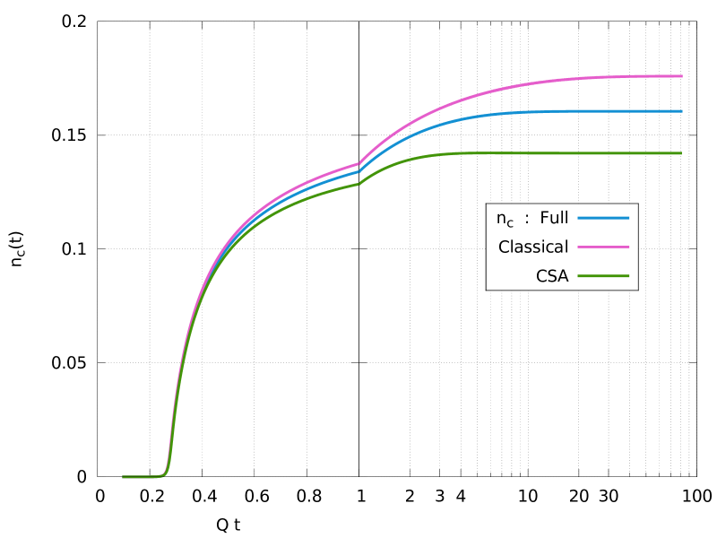
It appears that the three schemes agree qualitatively, and even semi-quantitatively, for the evolution of this quantity. The onset of condensation is almost exactly identical in all the schemes, while the final values of differ by about %. In agreement with the observations of ref. [32], the classical approximation tends to overpredict the fraction of condensed particles, while the classical statistical approximation tends to underpredict it.
Next, we consider the time evolution of the ratio between the transverse and longitudinal pressures. In Figure 16, we plot the time evolution of in the three schemes. Starting from a nonzero value dictated by the momentum anisotropy of the initial condition, this quantity is expected to return to zero as the particle distribution isotropizes.
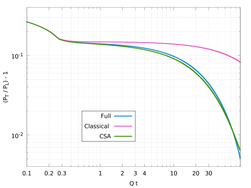
After a short initial stage during which the three schemes are nearly undistinguishable, we observe that the unapproximated scheme and the classical statistical approximation lead to almost identical time evolutions for this quantity, while the classical approximation isotropizes at a much slower pace. This is consistent with the argument exposed in the introduction, according to which the terms quadratic in are essential for out-of-plane scatterings in an anisotropic system.
Appendix B Integral of the product of four Bessel functions
B.1 Expression as an elliptic integral
In eq (20), we have encountered an integral involving the product of four Bessel functions,
| (71) |
which, to the best of our knowledge, does not seem to be known in the literature. In this appendix, we derive an exact expression of this integral in terms of an elliptic function , starting from the known expressions of similar integrals with two Bessel functions (see ref. [39]-6.512.8):
| (72) |
and three Bessel functions (see ref. [40]):
| (73) |
is the area of the triangle whose edges have lengths and (if such a triangle does not exist, then the integral is zero). We can therefore recast eq. (71) into the following expression:
| (74) |
Recall that the area of a triangle in terms of the lengths of its edges is given by the following formula,
| (75) | |||||
Thus, eq. (71) can be expressed as
| (76) |
where we denote and . The new integration variable is . The range of integration on is restricted by the fact that the arguments of the two square roots must both be positive:
| (77) |
Since it involves only a square root of a fourth degree polynomial, the integral in eq. (76) is an elliptic integral, which can be reduced to a combination of Legendre’s elliptic functions.
B.2 Expression in terms of the elliptic function
The boundaries of the integration range in eq. (76) are two of the roots of the polynomial
| (78) |
Let us call and these two roots, respectively the lower and upper bound. And for definiteness, let us call and the remaining two roots, arranged so that , i.e.
| (79) |
Eq. (71) is thus equivalent to
| (80) |
Let us now perform the following change of variables:
| (81) |
The above integral becomes
| (82) |
with and . This integral can be expressed in terms of the complete Legendre elliptic function of the first kind (defined for ),
| (83) |
which leads to the following compact expression151515From this formula, one can check the identity , that one expects from eqs. (71) and (73).
| (84) |
The function can be evaluated efficiently with a simple algorithm based on the arithmetic-geometric mean:
| (85) |
Figure 17 shows a comparison of a direct numerical evaluation of the integral in eq. (71) with the formula (84).
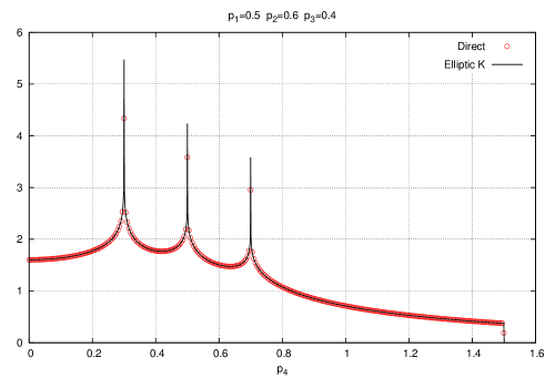
Note that this quantity becomes singular for special configurations of the ’s (in particular, when their values allow the vectors to become collinear). Near these points, the direct method is inefficient because of the very slow convergence of the integral. In contrast, eq. (84) is much better because the algorithm described in eqs. (85) converges to a very accurate result in only a few iterations161616The number of accurate digits doubles at every iteration.. Moreover, this method does not require the evaluation of any transcendental function.
Appendix C Integration domain for the collision term
When we discretize the collision integral of eq. (22), the domain of integration for the energy variables and is the one represented in Figure 18.
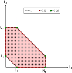
When or , this domain becomes a triangle. In this case, the points represented in green merge pairwise to form the summits of the triangle. The quadrature weight at these points becomes . But we do not need to handle this case by hand since the formula (50) gives the correct weights in all cases. Likewise, we have represented the integration domain on the longitudinal momenta and in Figure 19, with the quadrature weight of each point.
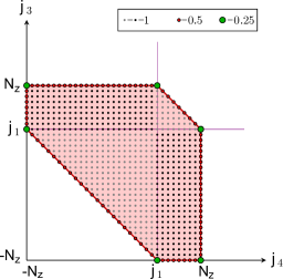
Since we have assumed that , the index is positive.
We need also to specify the integration domains for the terms and that describe collisions between a particle from the condensate and a particle at non-zero momentum, whose expressions are given in eq. (29). When , the integration over in is discretized as a sum over the following discrete points:
| (86) |
while for the longitudinal momentum we have:
| (87) |
For given in eq. (29), the integration domain for the energy is
| (88) |
while for the longitudinal momentum we have
| (89) |
Finally, we need also to specify the discrete domains in the right hand side of the equation (31) for the evolution of the particle density in the condensate. The sum over the energies and is over the following set of points:
![[Uncaptioned image]](/html/1506.05580/assets/x24.png)
|
and for the longitudinal momenta and it reads:
![[Uncaptioned image]](/html/1506.05580/assets/x25.png)
|
Appendix D Discretization of the free-streaming term
In this section we derive the weights (57) that enter into eq. (52). This derivation can be done in the case where there is no Bose-Einstein condensate, since the particles in the BEC carry zero momentum and are therefore not affected by free streaming. Let us start with the particle density defined in eq. (53). From the conservation of the number of particles, it should obey
| (90) |
Let us recall that eq. (52) is only valid for . Therefore, we first need to rewrite the particle density (53) by using the parity in (i.e. ) and the fact that
| (91) |
As one can see on Figure 5, particles can hop to the line from the left or from the right. Therefore, for , eq. (52) can be rewritten as follows:
| (92) | |||||
Then , by summing eqs. (52) and (92) on the indices , we obtain (the indices of the last two terms have been shifted)
| (93) |
The right-hand side must therefore be equal to that of eq. (91), for every . This leads first to
| (94) |
and
| (95) | |||||
Next, using the definition for the total energy (54) and the longitudinal pressure (55), we can use Bjorken’s law
| (96) |
in order to obtain
| (97) |
where we have denoted . This implies the following constraints among the coefficients :
| (98) |
The second of these constraints is incompatible with the first of eqs. (95), unless we set up the lattice spacings in such a way that the points do not satisfy the mass-shell condition (i.e. are below the red line in Figure 5), so that they do not contribute to and . From now on, we assume that this is the case. We do not explicitly exclude these points from the sums, but we simply assume that .
By comparing the second of eqs. (95) and the third of eqs. (98), we obtain
| (99) |
In order to fully constrain the coefficients, we need to consider also the total longitudinal momentum given in eq. (56), and impose its conservation:
| (100) |
This leads to
| (101) |
where we denote . From this equation, we obtain an additional constraint
| (102) |
Combining it with eqs. (95) and (99), we get finally
| (103) | |||||
| (104) |
Appendix E Direct simulation Monte-Carlo method
In this appendix, we present a generalization of the so-called direct simulation Monte Carlo (DSMC) method [41] to study the time-evolution of the distribution of relativistic particles and the formation of a Bose-Einstein condensate in a boost-invariant longitudinally expanding system. By including only the processes, the Boltzmann equation takes the following general form,
| (105) |
where the collision integral reads
| (106) | |||||
is the matrix element for the scattering process , and it simply reads for the theory. Let us parameterize the 3-momenta of the final state particles as follows:
| (107) |
where is a unit vector () and the total momentum
| (108) |
The conservation of energy gives
| (109) |
with and . By replacing by the new variables and and integrating out and , the Boltzmann equation can be shown to take the following form,
| (110) |
where is defined in eq. (14).
Eq. (E) can be solved by the direct simulation Monte-Carlo method. In this method, one defines a Markov process with a total number of simulated particles [41]. Let us introduce a partition (with ) of the momentum space into bins and denote the number of simulated particles with momentum in the momentum bin . The distribution function is then approximated by
| (111) |
where is the number density of “real” particles. In this paper, we assume that the system is homogeneous and isotropic in the transverse plane. Therefore, we adopt a partition of momentum space that divides the transverse momentum squared in equal intervals, , and likewise for the longitudinal momentum axis, , i.e.
| (112) |
Let us denote the momentum of the -th simulated particle by with . The probability for any two of the simulated particles and (with ) to scatter off each other during a time interval
| (113) |
is given by
| (114) |
where
| (115) | |||||
with , respectively the sums of energies and momenta of the particles and and and given by eqs. (107) (with and respectively replaced by and ). Here, can be chosen arbitrarily as long as it satisfies
| (116) |
For each time interval , the effect of the longitudinal expansion can be taken into account by simply rescaling the longitudinal momenta of all the simulated particles, according to
| (117) |
and
| (118) |
In situations where a BEC may form, we define as belonging to the condensate the simulated particles with momenta 171717This amounts to regularizing the delta function that would normally characterize the condensate by This choice makes our algorithm faster than the one used in the test particle method [42, 43] and hence better suited for the study of expanding systems.
| (119) |
and the number density of the condensate is defined as
| (120) |
with the number of condensate simulated particles that satisfy the condition (119). Note that this definition of the particles in the condensate includes both particles with exactly zero momentum (the “genuine” condensate), and the particles with non-zero momentum in a small volume around . When this extra volume is small enough, the above definition agrees well with an actual condensate. For all the results using DSMC in the expanding case have used the following parameters
| (121) |
The DSMC algorithm for solving the Boltzmann equation is made of the following steps:
-
i.
Choose randomly a pair of simulated particles (with a uniform probability distribution among all the possible pairs),
-
ii.
Choose a random vector (with an uniform distribution on the unit sphere),
-
iii.
Calculate and from and . If two or more momenta among and satisfy eq. (119), skip the step iv and go directly to v.
-
iv.
Choose a random number (with an uniform distribution). If , and are respectively replaced by and ,
- v.
-
vi.
Increment the time and return to the step i.
In order to illustrate this method and its difference with the deterministic method used in the rest of this paper, we have applied it to the case of a spatially homogeneous non-expanding system. In this case the Dirac function is regularized by and the momentum space is divided in equal intervals of the modulus of the momentum. The results of this comparison are shown in Figure 20.
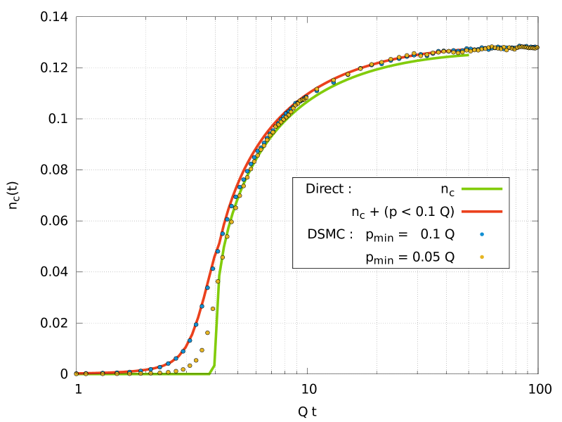
Because the operational definition of the condensate in the DSMC method also includes the particles in a small sphere of radius around , the transition of condensation appears less sharp than in the deterministic method where the density is defined as the coefficient of the delta function . By decreasing the value of the used in this definition, the transition in the DSMC simulation appears to become sharper, to finally become very close to the transition observed in the direct method. Alternatively, this interpretation can be further checked by adding to the of the deterministic method the contribution of the non-condensed particles contained in this small sphere.
References
- [1] J. Berges, K. Boguslavski, S. Schlichting, R. Venugopalan, Phys. Rev. D 89, 074011 (2014).
- [2] J. Berges, K. Boguslavski, S. Schlichting, R. Venugopalan, JHEP 1405, 054 (2014).
- [3] J. Berges, K. Boguslavski, S. Schlichting, R. Venugopalan, Phys. Rev. D 89, 114007 (2014).
- [4] J.P. Blaizot, F. Gelis, J. Liao, L. McLerran, R. Venugopalan, Nucl. Phys. A 873, 68 (2012).
- [5] K. Dusling, T. Epelbaum, F. Gelis, R. Venugopalan, Phys. Rev. D 86, 085040 (2012).
- [6] T. Epelbaum, F. Gelis, Phys. Rev. Lett. 111, 232301 (2013).
- [7] A. Kurkela, G.D. Moore, Phys. Rev. D 86, 056008 (2012).
- [8] A. Kurkela, G.D. Moore, JHEP 1112, 044 (2011).
- [9] A. Kurkela, E. Lu, Phys. Rev. Lett. 113, 182301 (2014).
- [10] M.P. Heller, D. Mateos, W. van der Schee, D. Trancanelli, Phys. Rev. Lett. 108, 191601 (2012).
- [11] M.P. Heller, D. Mateos, W. van der Schee, M. Triana, JHEP 1309, 026 (2013).
- [12] B. Wu, P. Romatschke, Int. J. Mod. Phys. C 22, 1317 (2011).
- [13] M.P. Heller, R.A. Janik, P. Witaszczyk, Phys. Rev. Lett. 108, 201602 (2012).
- [14] K. Fukushima, F. Gelis, Nucl. Phys. A 874, 108 (2012).
- [15] W. van der Schee, P. Romatschke, S. Pratt, Phys. Rev. Lett. 111, 22, 222302 (2013).
- [16] E. Iancu, A. Leonidov, L.D. McLerran, Lectures given at Cargese Summer School on QCD Perspectives on Hot and Dense Matter, Cargese, France, 6-18 Aug 2001, hep-ph/0202270.
- [17] E. Iancu, R. Venugopalan, Quark Gluon Plasma 3, Eds. R.C. Hwa and X.N. Wang, World Scientific, hep-ph/0303204.
- [18] H. Weigert, Prog. Part. Nucl. Phys. 55, 461 (2005).
- [19] F. Gelis, E. Iancu, J. Jalilian-Marian, R. Venugopalan, Ann. Rev. Part. Nucl. Sci. 60, 463 (2010).
- [20] F. Gelis, Int. J. Mod. Phys. A 28, 1330001 (2013).
- [21] A.H. Mueller, D.T. Son, Phys. Lett. B 582, 279 (2004).
- [22] S. Jeon, Phys. Rev. C 72, 014907 (2005).
- [23] V. Mathieu, A.H. Mueller, D.N. Triantafyllopoulos, Eur. Phys. J. C 74, 2873 (2014).
- [24] J. Berges, K. Boguslavski, S. Schlichting, R. Venugopalan, Phys. Rev. Lett. 114, 061601 (2015).
- [25] J. Berges, B. Schenke, S. Schlichting, R. Venugopalan, Nucl. Phys. A 931, 348 (2014).
- [26] D.V. Semikoz, I.I. Tkachev, Phys. Rev. Lett. 74, 3093 (1995).
- [27] D.V. Semikoz, I.I. Tkachev, Phys. Rev. D 55, 489 (1997).
- [28] T. Epelbaum, F. Gelis, Nucl. Phys. A 872, 210 (2011).
- [29] J.P. Blaizot, J. Liao, L.D. McLerran, Nucl. Phys. A 920, 58 (2013).
- [30] J.P. Blaizot, B. Wu, L. Yan, arXiv:1402.5049.
- [31] J. Berges, D. Sexty, Phys. Rev. Lett. 108, 161601 (2012).
- [32] T. Epelbaum, F. Gelis, N. Tanji, B. Wu, Phys. Rev. D 90, 125032 (2014).
- [33] T. Epelbaum, F. Gelis, B. Wu, Phys. Rev. D 90, 065029 (2014).
- [34] S. Jeon, Phys. Rev. D 47, 4586 (1993).
- [35] S. Jeon, Phys. Rev. D 52, 3591 (1995).
- [36] P. Arnold, G.D. Moore, L.G. Yaffe, JHEP 0011, 001 (2000).
- [37] A. Kurkela, Y. Zhu, arXiv:1506.06647.
- [38] P. Arnold, G.D. Moore, L.G. Yaffe, JHEP 0301, 030 (2003).
- [39] I.S. Gradshteyn, I.M. Ryzhik, Table of integrals, series and products, Academic Press, London (2000).
- [40] A. Gervois, H. Navelet, J. Math. Phys. 25, 3350 (1984).
- [41] A.L. Garcia, W. Wagner, Phys. Rev. E 68, 056703 (2003).
- [42] B. Jackson, E. Zaremba, Phys. Rev. A 66, 033606 (2002).
- [43] Z. Xu, K. Zhou, P. Zhuang, C. Greiner, Phys. Rev. Lett. 114, 182301 (2015).