Investigation of the Magnetic Model in Multiferroic NdFe₃(BO₃)₄ by Inelastic Neutron Scattering

Abstract

We performed inelastic neutron scattering measurements on single crystals of NdFe₃(¹¹BO₃)₄ to explore the magnetic excitations, to establish the underlying Hamiltonian, and to reveal the detailed nature of hybridization between the 4$f$ and 3$d$ magnetism. The observed spectra exhibiting a couple of key features, i.e., anti-crossing of Nd- and Fe-excitations and anisotropy gap at the antiferromagnetic zone center, are explained by the magnetic model including spin interaction in the framework of weakly-coupled Fe³⁺ chains, interaction between the Fe³⁺ and Nd³⁺ moments, and single-ion anisotropy derived from Nd³⁺ crystal field. The combination of the measurements and calculations reveals that the hybridization between 4$f$ and 3$d$ magnetism propagates the local magnetic anisotropy of the Nd³⁺ moment to the Fe³⁺ network, leading to the determination of the bulk structure of both electric polarization and magnetic moment in the multiferroics of the spin-dependent metal-ligand hybridization type.

I Introduction

Coexistence of magnetic order and electric polarization, multiferroicity, has become a major topic over the past decade in condensed matter physics. Since multiferroicity was originally discovered in perovskite TbMnO₃, nature426 various multiferroic compounds have been found, including $R$MnO₃ ($R$ = Eu, Gd, Tb, and Dy),PRL92_RMnO3 Ba_0.5Sr_1.5Zn₂Fe₁₂O₂₂, PRL94_BaSrZnFeO Ni₃V₂O₈, PRL95_Ni3V2O8 CoCr₂O₄, PRL96_CoCr2O4 MnWO₄, PRL97_MnWO4 CuFeO₂, PRB73_CuFeO2 LiCu₂O₂, PRL98_LiCu2O2 LiCuVO₄, JPSJ76_LiVCuO4 and Ba₂CoGe₂O₇. PRL105_Ba2CoGe2O7 Recent theoretical and experimental studies revealed that the electric polarization in these compounds is driven by magnetic long-range order. PRL95 ; PRL96 ; PRB73 ; PRB76 ; JPSJ76 Since the structure of the order is determined by the exchange pathways and the magnetic anisotropy, experimental identification of the magnetic Hamiltonian is very important for understanding multiferroics.

The rare-earth ferroborates $R$Fe₃(BO₃)₄ ($R$ = rare-earth metal) are a series of new multiferroic compounds containing $R^{3+}$ (4$f^{n}$) and Fe³⁺ (3$d^{5}$ $S=5/2$) as magnetic ions. The variety of the magnetic anisotropy of the $R^{3+}$ moments ($R$ = Y, Pr, Nd, Sm, Gd and Tb) combined with the interaction between the Fe³⁺ and $R^{3+}$ moments ($f$-$d$ coupling) gives rise to diverse magnetoelectric (ME) effects as a function of the $R^{3+}$ ions.JETP81 ; JETP83 ; JETP105 ; JETP109 ; LTP36 ; PRB82 In these compounds the mechanism of magnetoelectricity is explained by the spin-dependent metal-ligand hybridization model. PRB87 ; PRB89

The crystal structure has the trigonal space group $R32$, which belongs to the structural type of the mineral huntite CaMg₃(CO₃)₄. CM9 As shown in Fig. 1(a) the main feature is that distorted FeO₆ octahedra form spiral chains with threefold screw-axis symmetry along the crystallographic $c$ - axis. Each chain includes three Fe³⁺ ions in the unit cell. The chains are separated by the $R^{3+}$ and B³⁺ ions.

In NdFe₃(BO₃)₄ the Nd³⁺ ions (4$f^{3}$) carry magnetic moment with $J=9/2$. The magnetic susceptibility showed anisotropic decrease below 29 K, and the heat capacity showed well-defined $\lambda$ type anomaly at the same temperature, implying a phase transition to an antiferromagnetic (AF) ordered state with Néel temperature of $T_{N}=29$ K. MMM316 At $T\geq T_{N}$ the susceptibility is concave downward, indicating the short-range AF order because of the low dimensionality of the magnetic system. Spontaneous electric polarization simultaneously appears in the AF ordered phase. LTP36 The electric polarization significantly increases upon applying a magnetic field parallel to the $a$ - axis. The magnitude of the electric polarization reaches $P_{a}\sim 300$ $\mu$C/m² at 1.3 T and 4.2 K, JETP83 ; JETP105 which means that the magnetization along the $a$ - axis induces the large electric polarization along the $a$ - axis. A neutron diffraction study exhibited an easy-plane type AF order at $T\leq T_{N}$; the Fe³⁺ and Nd³⁺ magnetic moments align ferromagnetically along the $a$ - axis and propagate antiferromagnetically along the $c$ - axis with the propagation vector $k$ = (0, 0, 3/2) in Fig. 1(a). JPCM18 ; PRB81 Both of Fe³⁺ and Nd³⁺ moments are simultaneously ordered at the $T_{N}$, indicating non-negligible $f$-$d$ coupling. Further decreasing the temperature at $T\leq T_{{\rm IC}}=13.5$ K, the commensurate (C) magnetic peak splits into a pair of incommensurate (IC) peaks where the magnetic moments are in the $ab$ - plane and the AF helix propagates along the $c$ - axis.

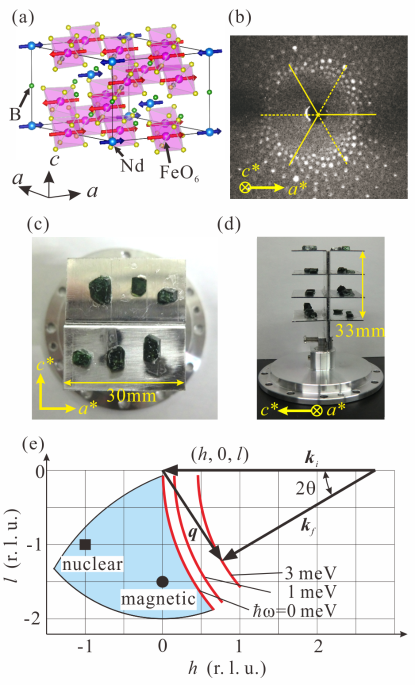
Figure 1: (Color online) (a) The crystal structure and magnetic structure of NdFe₃(BO₃)₄ (hexagonal, space-group $R32$). (b) Laue image of a crystal with the $c^{\ast}$ - axis parallel to the incident X-ray beam. Crystals of NdFe₃(¹¹BO₃)₄ on the alumina holder viewed from above (c) and from the side (d). (e) Reciprocal space in the $a^{\ast}$ - $c^{\ast}$ plane. The square at $(h,k,l)=(-1,0,-1)$ is a nuclear Bragg reflection. The circle at $(0,0,-1.5)$ is a magnetic Bragg reflection. Red curves indicate spectra measured with $\mbox{\boldmath$k$}_{i}//a^{\ast}$ for $\hbar\omega=0,1$ and 3 meV. The blue shaded area indicates the range of the observed scattering plane for $k_{i}=2.352$ Å^-1 and $\hbar\omega=0$ meV when sample is rotated.

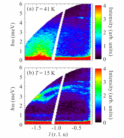
Figure 2: (Color online) Inelastic neutron spectra projected onto $c^{\ast}$ - axis at (a) 41 K and (b) 15 K. The incident neutron energy was 11.46 meV.

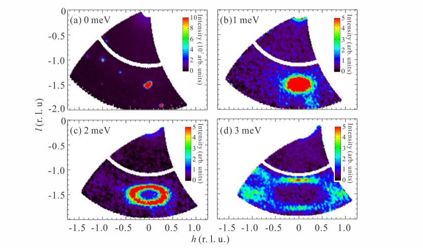
Figure 3: (Color online) Constant energy cuts at 0 meV (a), 1 meV (b), 2 meV (c) and 3 meV (d) in the $a^{\ast}$ - $c^{\ast}$ plane. The horizontal and vertical axes represent the $a^{\ast}$ and $c^{\ast}$ axes, respectively

Magnetic dynamics have been investigated by spectroscopic methods using electromagnetic waves. ESR measurement detected an energy gap suggesting a uniaxial magnetic anisotropy in the $ab$ - plane. JETP94 It also detected lifting of the Kramers doublet of the Nd³⁺ ion due to the molecular field from the neighboring Fe³⁺ ions. Optical spectroscopy provided the energy levels of the crystal field of the Nd³⁺ ion and determined the parameters of the crystal field Hamiltonian. PRB75

In NdFe₃(BO₃)₄ exhibiting the strong $f$-$d$ coupling, the investigation of excitation spectra including Fe³⁺ spin wave and Nd³⁺ crystal field in a wide wave-vector energy space is crucial in order to identify the magnetic Hamiltonian and to unravel the detailed nature of hybridization between 3$d$ and 4$f$ magnetism. Furthermore in constructing the Hamiltonian, careful consideration of magnetic anisotropy is important in the multiferroics of the spin-dependent metal-ligand hybridization mechanism type,PRB76 ; JPSJ76 in which the magnetic anisotropy directly determines the polarization structure.

In the present paper we study inelastic neutron scattering (INS) spectra on NdFe₃(¹¹BO₃)₄ to explore the magnetic excitations and to establish the underlying Hamiltonian. Following to the introduction we describe the experimental details about the sample preparation and the setup of INS measurements in Sec. II. Subsequently in Sec. III the INS spectra of NdFe₃(¹¹BO₃)₄ are demonstrated. We observed spin waves of the Fe³⁺ moment below 6 meV and transition between the lifted states of Kramers doublet of the Nd³⁺ ion at 1 meV. A couple of characteristic features are an anti-crossing of the Fe- and Nd-excitations, and a small anisotropy gap at the antiferromagnetic zone center. In Sec. IV the magnetic model including an in-plane anisotropy derived from the crystal field excitation of the Nd³⁺ moment and the non-negligible $f$-$d$ coupling is constructed. The observed spectra are successfully analyzed by the linear spin wave theory based on the model. The origin of the in-plane anisotropy is revealed to be the crystal field of the Nd³⁺ ion. In Sec. V possibility of magnetic anisotropy of the Fe³⁺ moment is discussed. It is turned out that the anisotropy is very small, and, instead, the Fe³⁺ moment inherits an in-plane anisotropy through hybridization with the Nd³⁺ moment. The conclusions are given in Sec. VI. The magnetic Hamiltonian in NdFe₃(¹¹BO₃)₄ is established in the present study. Combination of the measurement and the detailed calculation revealed that the hybridization between 4$f$ and 3$d$ magnetism propagates the local magnetic anisotropy of the Nd³⁺ ion to the Fe³⁺ network, resulting in the bulk structure of multiferroics. The local symmetry of the rare-earth ion is a driving force for the non-local multiferroicity in NdFe₃(¹¹BO₃)₄.

II Experimental details

Single crystals of NdFe₃(¹¹BO₃)₄ were grown by a flux method.flux We first synthesized polycrystalline samples from the starting materials, Nd₂O₃, Fe₂O₃, and ¹¹B₂O₃. The stoichiometric amounts of the starting materials with a total mass of about 16 g were mixed, ground, and put into an alumina crucible. The crucible was heated at 980 ^∘C for 72 h. The flux is Bi₂Mo₃O₁₂ + 3 ¹¹B₂O₃ + 3/5 Nd₂O₃; Bi₂Mo₃O₁₂ was synthesized by the solid state reaction from Bi₂O₃ and MoO₃ inside an alumina crucible at 600 ^∘C for 24 h. A mixture of about 60 g of NdFe₃(¹¹BO₃)₄ and the flux with the mass ratio of 1 : 3 was put into a platinum crucible inside the alumina crucible. The crucible was heated to 1000 ^∘C for 4 h, kept at this temperature for 1 h, cooled to 962 ^∘C for 1 h, and slowly cooled down to 870 ^∘C for 120 h; then the furnace was shut down to the room temperature. The flux was removed by decanting at 900 ^∘C, and washing the crystals with HCl solutions.

We coaligned 22 pieces of single crystals so that the crystallographic $a^{\ast}$ - $c^{\ast}$ plane is horizontal. Alignment was performed by transmission Laue method using a high energy X-ray Laue camera. The X-ray source was YXLON MG452 and the maximum energy of the white X-ray beam was 310 keV. We recorded Laue patterns using a high-speed CCD camera, with imaging size 10 cm $\times$ 10 cm (1024 $\times$ 1024 pixel). Figure 1(b) shows a Laue image of a crystal in the $c^{\ast}$ - plane. This pattern exhibits the threefold symmetry along the $c^{\ast}$ - axis. We placed the crystals on an alumina holder as shown in Figs. 1(c) and 1(d). The average mass of the crystals was 0.1 g. The total mass of the sample was 2.1 g.

The INS experiment was performed at the High Resolution Chopper Spectrometer (HRC) installed in the Material and Life Science Experimental Facility of J-PARC. NI631 ; NI654 ; JPSJ82 At the HRC white neutrons are monochromatized by a Fermi chopper synchronized with the production timing of the pulsed neutrons. The energy transfer $\hbar\omega$ was determined from the time of flight (TOF) of the scattered neutrons detected at position sensitive detectors (PSDs). The T₀ chopper was set at 50 Hz, a collimator of 1.5^∘ was installed in front of the sample, and the “S” Fermi chopper with 200 Hz was used to obtain high neutron flux. We used a GM-type closed cycle cryostat to achieve 41 K and 15 K. The energy of the incident neutron beam was $E_{i}=11.46$ meV yielding an energy resolution of $\Delta E=0.3$ meV at the elastic position.

Figure 1(e) illustrates the $a^{\ast}$ - $c^{\ast}$ scattering plane. Reciprocal lattice positions at $\mbox{\boldmath$q$}=(-1,0,-1)$ and $(0,0,-1.5)$ are the positions of nuclear and magnetic Bragg peaks, respectively. Throughout this paper $q$ is expressed in reciprocal lattice unit, $\mbox{\boldmath$q$}=(h,k,l)$. INS spectra with $\mbox{\boldmath$k$}_{i}//a^{\ast}$ were measured at 41 K and 15 K. Red curves in Fig. 1(e) indicate the measured $q$-ranges for $\hbar\omega=0,1$ and 3 meV. At 15 K INS spectra that cover wide $q$-range were measured by rotating the crystal by 70 degree in 2 degree steps. The $q$-range in the scan for $\hbar\omega=0$ meV is indicated by the blue shaded area in Fig. 1(e). The range of out of plane momentum is $|q_{\perp}|<0.41$ Å^-1. In the following, the out of plane spectra are integrated in the central range $|q_{\perp}|<0.13$ Å^-1, and we show all spectra in the $(h,0,l)$ plane.

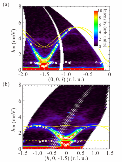
Figure 4: (Color online) Color maps of the inelastic neutron scattering spectra obtained at HRC, along the (a) $l$ and (b) $h$ directions at 15 K. The open circles are the peak positions extracted Gaussian fits and the curves are the calculated spin wave dispersions. Fitting curves reasonably reproduce the experimental data. White area in the middle in the panel (a) is the gap between neutron detectors banks.

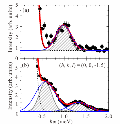
Figure 5: (Color online) (a) $\hbar\omega$ dependence of the neutron intensity that is obtained by the integration in the $q$-range of $h=[-0.5,0]$ and $l=[-1,-0.7]$. The solid curve is fit to the data by Gaussian functions. (b) Constant-$Q$ scan at $(0,0,-1.5)$. The spectra were integrated in the range of $h=[-0.1,0.1]$ and $l=[-1.6,-1.4]$. The error bars are inside the symbols. The solid curves are fits to the data by Gaussian functions. The gray shaded areas are the energy resolutions: Gaussian functions with full width at half maximum of 0.3 meV.

III Experimental results

The INS spectra projected onto the $c^{\ast}$ - axis at 41 K and 15 K are shown in Figs. 2(a) and 2(b), respectively. At 41 K a diffuse spectrum of paramagnetic scattering emerges from $l=-1.5$. At 15 K dispersive excitations emerge in the energy range of 2.5 meV $<\hbar\omega<4.5$ meV, which is interpreted as spin waves of the Fe³⁺ moments.

Figures 3(a)-3(d) display neutron spectra at 15 K sliced at the energies of 0, 1, 2, and 3 meV in the $a^{\ast}$ - $c^{\ast}$ plane. The white arcs are because of the absence of the neutron detectors between the detector banks. In Fig. 3(a) the peak at $\mbox{\boldmath$q$}=(-1,0,-1)$ is a nuclear Bragg reflection, and the peak at $(0,0,-1.5)$ is a magnetic Bragg reflection. The peaks at other $q$s are not identified; they may be Bragg reflection from minor grains of crystals. The rings expanding from $(0,0,-1.5)$ in Figs. 3(b)-3(d) imply that a dispersive excitation appears from $(0,0,-1.5)$. The rings are flattened along the $c^{\ast}$ - axis, which means that the dispersion along the $c^{\ast}$ - axis is steeper than that along the $a^{\ast}$ - axis. This is consistent with the naive prediction from the crystal structure that the intrachain interaction along the $c$ - axis is strong compared with the interchain interaction.

The INS spectrum at 15 K projected onto $\hbar\omega$ - $(0,0,l)$ plane by the integrating the neutron intensity in the ranges of $-0.1a^{*}\leq q\leq 0.1a^{*}$ along the ${\bm{a}^{*}}$ direction in the scattering plane and $-0.17a^{*}\leq q\leq 0.17a^{*}$ perpendicular to the scattering plane is shown in Fig. 4(a). The spectrum projected onto $\hbar\omega$ - $(h,0,-1.5)$ plane by the integration in the ranges of $-0.17a^{*}\leq q\leq 0.17a^{*}$ perpendicular to the scattering plane and $-1.6c^{*}\leq q\leq-1.4c^{*}$ along the ${\bm{c}^{*}}$ direction is shown in Fig. 4(b). We clearly observed the spin waves of the Fe³⁺ moments around $\mbox{\boldmath$q$}=(0,0,-1.5)$, and the flat excitation at about $1.0$ meV which is the transition between the lifted states of Kramers doublet of the Nd³⁺ ion. The spin waves of the Fe³⁺ moments are more dispersive along the $c^{\ast}$ direction than along the $a^{\ast}$ direction, which is consistent with the flattened ring in Figs. 3(b)-3(d).

A series of $\hbar\omega$ dependence of the neutron intensity obtained by the integration in the same $q$-ranges that were used for the display of Figs. 4(a) and 4(b) were fitted by Gaussian functions to investigate the detailed structures of the excitations. The peak energies were plotted as open circles in Figs. 4(a) and 4(b). These data will be used in the analysis section. The white circles around $\mbox{\boldmath$q$}=(0,0,-1.5)$ exhibit an anti-crossing between the spin wave of the Fe³⁺ moments and the flat mode of the Nd³⁺ moments, meaning that the Fe³⁺ moments interact with the Nd³⁺ moments.

Figure 5(a) shows the $\hbar\omega$ dependence of the neutron intensity obtained by the integration in the $q$-range of $h=[-0.5,0]$ and $l=[-1,-0.7]$, where the Nd³⁺-based mode is not affected by the Fe³⁺-based spin-wave mode. The dashed curve is incoherent elastic scattering and the blue curve is a Gaussian fit. The red curve is the sum of the dashed and blue curves. The gray shaded area is the energy resolution. From the peak position we identify the magnitude of the energy split of the Kramers doublet to be 0.98 meV. Figure 5(b) shows a constant-$q$ scan at $(0,0,-1.5)$, the AF zone center, that is obtained by integration in the $q$-range of $h=[-0.1,0.1]$ and $l=[-1.6,-1.4]$. The dashed curve is incoherent elastic scattering, the blue curves are Gaussian fits, and the red curve is the sum of the dashed and blue curves. The gray shaded areas indicate the energy resolutions. The magnitude of the energy gap at the AF zone center is estimated as $0.57$ meV. The gap implies the existence of an anisotropy in the $ab$ - plane. The excitation at 1.3 meV is the transition between the split of Kramers doublet of the Nd³⁺ ion. The peak energies of the Nd³⁺ ion in Fig. 5(a) and Fig. 5(b) are obviously different. The energy difference is due to the hybridization between the Fe³⁺ and Nd³⁺ modes. The energy widths of the excitations at $\hbar\omega=$ $0.57$ meV and 1.3 meV are broader than the experimental resolution. The energy split of $0.98$ meV and the energy gap of $0.57$ meV are consistent with the magnetic excitations reported from ESR measurement JETP94 and optical spectroscopy. PRB75

IV Analysis

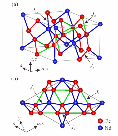
Figure 6: (Color online) Exchange paths in NdFe₃(BO₃)₄. $J_{1}$ and $J_{2}$ are the nearest and 2nd nearest neighbor exchange interactions between the Fe³⁺ moments. $J_{3}$ is the nearest neighbor exchange interaction between the Fe³⁺ and Nd³⁺ moments. The $x$ - axis is parallel to the $a$ - axis and the $z$ - axis is parallel to the $c$ - axis. The $y$ - axis is vertical to the $x$ and $z$ - axis.

In order to identify the magnetic model realized in NdFe₃(¹¹BO₃)₄, we consider the following Hamiltonian:

$${\cal H}=-\sum_{{\rm n.n.}}J_{1}\mbox{\boldmath$S$}_{i}\cdot\mbox{\boldmath$S$}_{j}-\sum_{{\rm n.n.n.}}J_{2}\mbox{\boldmath$S$}_{i}\cdot\mbox{\boldmath$S$}_{j}$$

$$-\sum_{{\rm n.n.}}J_{3}\mbox{\boldmath$S$}_{i}\cdot\mbox{\boldmath$J$}_{k}+\sum_{k}{\cal H}_{{\rm CF}}(\mbox{\boldmath$J$}_{k}),$$ (1)

where the $x$ - axis is parallel to the crystallographic $a$ - axis and the $z$ - axis is parallel to the $c$ - axis. $J_{1}$ and $J_{2}$ are the exchange interactions in the nearest and 2nd neighbor paths of the Fe³⁺ ions as shown in Figs. 6(a) and 6(b). These terms mainly determine the dispersions along the $c^{\ast}$ - axis and $a^{\ast}$ - axis, respectively. $J_{3}$ is the nearest neighbor exchange interaction between the Fe³⁺ and Nd³⁺ moments, which induces the anti-crossing between the Fe³⁺ and Nd³⁺ modes. In Eq. (1), positive (negative) signs of the exchange parameters correspond to ferromagnetic (antiferromagnetic) exchange interactions. ${\cal H}_{{\rm CF}}$ is the crystal field Hamiltonian of the Nd³⁺ ion.

There are five Kramers doublets in the crystal field of the Nd³⁺ ion above $T_{{\rm N}}=30$ K. The first excited energy is about 8 meV, and second one is about 17 meV as reported in Ref. PRB75, . In the calculation of the low-energy excitations below 6 meV it is assumed that only the ground state in the crystal field of the Nd³⁺ ion hybridizes with the Fe³⁺ moments. For this assumption, we introduce the ground state of the crystal field of the Nd³⁺ ion.

At the Nd³⁺ site with $D_{3}$ symmetry, the crystal field Hamiltonian can be defined as follow:

$${\cal H}_{{\rm CF}}=B^{2}_{0}C^{2}_{0}+B^{4}_{0}C^{4}_{0}+iB^{4}_{3}(C^{4}_{3}+C^{4}_{-3})$$

$$+B^{6}_{0}C^{6}_{0}+iB^{6}_{3}(C^{6}_{3}+C^{6}_{-3})+B^{6}_{6}(C^{6}_{6}+C^{6}_{-6}).$$ (2)

The $B^{p}_{q}$ are the crystal field parameters and the $C^{p}_{q}$ are the spherical tensor operators. We used the values of the parameter $B^{p}_{q}$ reported in Ref. PRB75, . Matrix elements of $J^{x}$, $J^{y}$, and $J^{z}$ in the ground state doublet $\ket{g_{\pm}}$ are as follow:

$$\left\{\begin{array}[]{l}\displaystyle{\bra{g_{\mp}}J^{x}\ket{g_{\pm}}=-1.67\equiv\frac{\beta}{2},}\\ \displaystyle{\bra{g_{\mp}}J^{y}\ket{g_{\pm}}=\pm\frac{\beta}{2}i}\\ \displaystyle{\bra{g_{\pm}}J^{z}\ket{g_{\pm}}=\mp 0.98\equiv\mp\frac{\alpha}{2},}\\ \displaystyle{\bra{g_{\pm}}J^{x}\ket{g_{\pm}}=\bra{g_{\pm}}J^{y}\ket{g_{\pm}}=\bra{g_{\mp}}J^{z}\ket{g_{\pm}}=0,}\end{array}\right.$$ (7)

meaning that the total angular momentum is anisotropic, favoring in-plane. Next we inspect anisotropy within the $ab$ - plane. The quantization axis is transformed from the $z$ - axis to the $x$ - axis because the direction of the spin in the order state is along the $x(a)$ - axis. Then, the matrix elements of $J^{x}$, $J^{y}$, and $J^{z}$ in the redefined state $\ket{g_{\pm}^{\prime}}$ are calculated as follow:

$$\left\{\begin{array}[]{l}\displaystyle{\bra{g_{\pm}^{\prime}}J^{x}\ket{g_{\pm}^{\prime}}=\mp\frac{\beta}{2},}\\ \displaystyle{\bra{g_{\mp}^{\prime}}J^{y}\ket{g_{\pm}^{\prime}}=\frac{\beta}{2},}\\ \displaystyle{\bra{g_{\mp}^{\prime}}J^{z}\ket{g_{\pm}^{\prime}}=\pm\frac{\alpha}{2}i,}\\ \displaystyle{\bra{g_{\mp}^{\prime}}J^{x}\ket{g_{\pm}^{\prime}}=\bra{g_{\pm}^{\prime}}J^{y}\ket{g_{\pm}^{\prime}}=\bra{g_{\pm}^{\prime}}J^{z}\ket{g_{\pm}^{\prime}}=0.}\end{array}\right.$$ (12)

The operator $B^{6}_{6}(C^{6}_{6}+C^{6}_{-6})$ leads to an anisotropy within the $ab$ - plane. In order to quantify this, we express the total angular momentum of the Nd³⁺ ion in the ground state doublet as

$$J^{x}=\frac{\beta}{2}\cos\theta,\quad J^{y}=\frac{\beta}{2}\sin\theta,$$ (13)

where $\theta$ is the angle between the $a$ - axis and the moment. Thus classical energy of $B^{6}_{6}(C^{6}_{6}+C^{6}_{-6})$ becomes

$$B_{6}^{6}\left(C_{6}^{6}+C_{-6}^{6}\right)=\frac{\sqrt{231}}{16}B_{6}^{6}\gamma_{J}\left(\frac{\beta}{2}\right)^{6}\cos 6\theta,$$ (14)

where $\gamma_{J}=-3.80\times 10^{-5}$ is a Stevens’ factor. Eq. (14) means that the classical energy of the crystal field gives a six-fold anisotropy. Since the sign of the $B_{6}^{6}\gamma_{J}$ is negative, the easy-axis is the $a$ - axis that is consistent with the magnetic structure.PRB81 The magnitude of the calculated anisotropy energy is $65.2$ $\mu$eV. We effectively include the six-fold anisotropic energy as $-D\left(J^{x}\right)^{2}$ in the Hamiltonian Eq. (1). The coefficient $D$ is $23.5$ $\mu$eV, which is defined by the relation:

$$-D\left(\frac{\beta}{2}\right)^{2}\equiv\frac{\sqrt{231}}{16}B_{6}^{6}\gamma_{J}\left(\frac{\beta}{2}\right)^{6}\times 2=65.2\hskip 5.0pt\mu{\rm eV}.$$ (15)

Next the operators of total angular momentum $J$ are approximated as the operators of pseudo-spin $s=1/2$ because the ground state is Kramers doublet and the degree of freedom is two. The connection between operators of the total angular momentum $J$ and the pseudo-spin $s$ is determined by the matrix elements Eq. (12). In this approximation the operators of the total angular momentum is redefined as

$$J^{x}=\beta s^{x},\quad J^{y}=\beta s^{y},\quad J^{z}=\alpha s^{z}.$$ (16)

The Hamiltonian Eq. (1) is, thus, represented by

$${\cal H} = -\sum_{{\rm n.n.}}J_{1}\mbox{\boldmath$S$}_{i}\cdot\mbox{\boldmath$S$}_{j}-\sum_{{\rm n.n.n.}}J_{2}\mbox{\boldmath$S$}_{i}\cdot\mbox{\boldmath$S$}_{j}$$ (20)

$$-\sum_{{\rm n.n.}}J_{3}\mbox{\boldmath$S$}_{i}\cdot\left(\begin{array}[]{c}\displaystyle{\beta s_{k}^{x}}\\ \displaystyle{\beta s_{k}^{y}}\\ \displaystyle{\alpha s_{k}^{z}}\end{array}\right)-\sum_{k}D\left(\beta s_{k}^{x}\right)^{2}.$$

We subsequently calculate the spin wave spectrum of this Hamiltonian using Holstein-Primakoff (HP) transformations. The HP transformations of the spin operators of the Fe³⁺ moments and the pseudo-spin operators of the Nd³⁺ moments are written as

$$S^{x}_{i} = S-a^{\dagger}_{i}a_{i},$$ (21)

$$S^{y}_{i} = \sqrt{\frac{S}{2}}\left(a_{i}^{\dagger}+a_{i}\right),$$ (22)

$$S^{z}_{i} = -\sqrt{\frac{S}{2}}i\left(a_{i}^{\dagger}-a_{i}\right),$$ (23)

$$s^{x}_{i} = s-b^{\dagger}_{i}b_{i},$$ (24)

$$s^{y}_{i} = \sqrt{\frac{s}{2}}\left(b_{i}^{\dagger}+b_{i}\right),$$ (25)

$$s^{z}_{i} = -\sqrt{\frac{s}{2}}i\left(b_{i}^{\dagger}-b_{i}\right).$$ (26)

The $a^{\dagger}_{i},a_{i},b^{\dagger}_{i}$ and $b_{i}$ are bosons operator in each sublattices. The quantization axis is parallel to the $x(a)$ - axis. We introduce spatial Fourier transformation via

$$c_{i}^{\dagger}(\mbox{\boldmath$q$})=\frac{1}{\sqrt{N}}\sum_{\mbox{\boldmath$r$}_{i}}c_{i}^{\dagger}e^{-i\mbox{\boldmath$q$}\cdot\mbox{\boldmath$r$}_{i}}\quad(i=1\sim 24),$$ (27)

where $N$ is the number of unit cells in the system, and $\{c_{i}\}=\{a_{i},b_{i}\}$ are the bosons operators on each sublattice. By using this notation we obtain

$${\cal H} = \sum_{\mbox{\boldmath$q$}}\sum_{ij}A_{ij}(\mbox{\boldmath$q$})c_{i}^{\dagger}(\mbox{\boldmath$q$})c_{j}(\mbox{\boldmath$q$})$$ (28)

$$+\frac{1}{2}\sum_{ij}\left[B_{ij}(\mbox{\boldmath$q$})c_{i}^{\dagger}(\mbox{\boldmath$q$})c_{j}^{\dagger}(\mbox{\boldmath$q$})+{\rm h.c.}\right].$$

The eigenvalues of the matrix $\left(\mbox{\boldmath$A$}+\mbox{\boldmath$B$}\right)\left(\mbox{\boldmath$A$}-\mbox{\boldmath$B$}\right)$ give the squares of the energy of the normal modes PRB56 :

$$\left(\mbox{\boldmath$A$}+\mbox{\boldmath$B$}\right)\left(\mbox{\boldmath$A$}-\mbox{\boldmath$B$}\right)\chi_{\tau}(\mbox{\boldmath$q$})=\left\{\hbar\omega(\mbox{\boldmath$q$})\right\}^{2}\chi_{\tau}(\mbox{\boldmath$q$}).$$ (29)

The dispersions obtained from this calculation are indicated by the yellow solid curves in Figs. 4(a) and 4(b). In fact we obtained 24 modes of spin waves, but due to the trigonal symmetry of the lattice only 8 modes have non-zero spectral weight. The modes at the highest and second-highest energies around the AF zone center, ${\mbox{\boldmath$q$}}=(0,0,-1.5)$, in Fig. 4(a) are two-fold degenerated, and the highest energy mode in Fig. 4(b) is four-fold degenerated. At the zone center, there are two modes at $\hbar\omega=1.12$ meV and $1.23$ meV, and another two modes at $\hbar\omega=0.32$ meV and $0.61$ meV. The $0.32$ meV gap is caused by the anisotropy of the Nd³⁺ moment in the $ab$ plane. It vanishes if the $D$ is set to zero. The modes at $1.12$ meV and $1.23$ meV is the Nd³⁺ level after hybridizing with the dispersive Fe³⁺ spin waves. The small splittings of both modes are due to the easy-plane type anisotropy of the Nd³⁺ ion, i.e., the effect of $\alpha\neq\beta$. These splittings are the origin of the observed broadenings of the experimental peaks in Fig. 5(b). White circles in Figs. 4(a) and 4(b) are fit by the mean energy of the split modes. ${\chi}^{2}$s were calculated for the parameter set with the step sizes of $\delta J_{1}=0.001$ meV, $\delta J_{2}=0.001$ meV, and $\delta J_{3}=0.1$ $\mu$eV in the ranges of $|J_{1}|\leq 1$ meV, $|J_{2}|\leq 1$ meV, and $|J_{3}|\leq 0.1$ meV. The obtained parameters set for the minimum ${\chi}^{2}$ is listed in Table 1. The fit to the data provides excellent agreement with the overall spectrum. It should be noted that the anisotropy gap of about $0.57$ meV at the zone center is quantitatively reproduced by using the fixed parameter of $D$ = 23.5 $\mu$eV obtained from reported value of the parameter $B_{6}^{6}$.PRB75 It is revealed that the origin of the in-plane anisotropy is the crystal field of the Nd³⁺ ion.

Table 1: Parameters obtained by the linear spin wave calculations

$J_{1}$ [meV]	$J_{2}$ [meV]	$J_{3}$ [$\mu$eV]	$D$ [$\mu$eV] (fixed)	$\chi^{2}$
$-0.482$	$-0.054$	$7.9$	$23.5$	$0.993$

V Discussion

In $R$Fe₃(BO₃)₄, the magnitude of the electric polarization by the $R^{3+}$ and Fe³⁺ ions are locally determined by the magnetic moments.PRB87 ; PRB89 In case of NdFe₃(BO₃)₄ the existence of the in-plane anisotropy favoring order along the $a$ - axis by the Nd³⁺ and/or Fe³⁺ ions is a key to the emergence of the multiferroicity. In the analysis section, uniaxial anisotropy of the Fe³⁺ moments is not considered for the simplicity. In this section, we discuss possible magnetic anisotropies in the $ab$ - plane of the Fe³⁺ moments.

The conventional origin of anisotropy in Fe³⁺-based magnets is magnetic-dipole interaction or single-ion anisotropy. The magnetic-dipole interaction between spins $\mbox{\boldmath$S$}_{i}$ and $\mbox{\boldmath$S$}_{j}$ is represented by

$${\cal H}_{\rm dip}=\sum_{i,j}\frac{\left(g\mu_{\rm B}\right)^{2}}{r_{ij}^{3}}\left\{\mbox{\boldmath$S$}_{i}\cdot\mbox{\boldmath$S$}_{j}-3\left(\mbox{\boldmath$S$}_{i}\cdot\mbox{\boldmath$e$}_{ij}\right)\left(\mbox{\boldmath$S$}_{j}\cdot\mbox{\boldmath$e$}_{ij}\right)\right\},$$ (30)

where $r_{ij}$ and $\mbox{\boldmath$e$}_{ij}$ are respectively the distance and the unit vector along the bond between $i$ and $j$. For a collinear in the $ab$ - plane, the dipole-interaction energy is independent of the angle to the $a$ - axis. This is due to the threefold screw-axis symmetry along the $c$ - axis, which also dictates that further neighbor interactions vanish. Thus, the magnetic-dipole interaction is not the origin of the anisotropy in the $ab$ - plane.

Next, we consider the single-ion anisotropy of the Fe³⁺ moments. There is only one inequivalent site for the Fe³⁺ ion and the local anisotropy is uniquely determined. Since the screw axis $3_{1}$ or $3_{2}$ is along the Fe³⁺ chain, the FeO₆ octahedra are transformed by $2\pi/3$ rotation around the $c$ - axis one another. Therefore, three local coordinates, $\left\{X_{i},Y_{i},Z_{i}\right\}$, can be defined on the FeO₆ octahedra for the anisotropy. Here $\{i=1,2,3\}$ are the labels of the Fe³⁺ sites. Since the Fe³⁺ moments are collinear in the $ab$ - plane, we discuss the anisotropy only in the $ab$ - plane. Then, the general single-ion anisotropy to 4th order in the Fe³⁺ spin-operators is expressed by

$${\cal H}_{{\rm aniso}}=\sum_{i=1,2,3}\left[a_{x^{2}}\left(S_{i}^{X_{i}}\right)^{2}+a_{y^{2}}\left(S_{i}^{Y_{i}}\right)^{2}+a_{xy}S_{i}^{X_{i}}S_{i}^{Y_{i}}\right.$$ (31)

$$+a_{x^{4}}\left(S_{i}^{X_{i}}\right)^{4}+a_{y^{4}}\left(S_{i}^{Y_{i}}\right)^{4}+a_{x^{2}y^{2}}\left(S_{i}^{X_{i}}\right)^{2}\left(S_{i}^{Y_{i}}\right)^{2}$$

$$\left.+a_{x^{3}y}\left(S_{i}^{X_{i}}\right)^{3}S_{i}^{Y_{i}}+a_{xy^{3}}S_{i}^{X_{i}}\left(S_{i}^{Y_{i}}\right)^{3}\right].$$

The $a_{x^{2}}$, $a_{y^{2}}$, $a_{xy}$, $a_{x^{4}}$, $a_{y^{4}}$, $a_{x^{2}y^{2}}$, $a_{x^{3}y}$, and $a_{xy^{3}}$ are independent coefficients. Here we define the the local coordinate $\{X_{1},Y_{1},Z_{1}\}$ as the same as the global one $\{x,y,z\}$. Then the relation between the spin operators defined on the local coordinates $\{X_{2,3},Y_{2,3},Z_{2,3}\}$ and the those defined on the global one is as follows:

$$\left\{\begin{array}[]{l}\displaystyle{S_{2}^{X_{2}}=-\frac{1}{2}S_{2}^{x}+\frac{\sqrt{3}}{2}S_{2}^{y},}\\ \displaystyle{S_{2}^{Y_{2}}=-\frac{\sqrt{3}}{2}S_{2}^{x}-\frac{1}{2}S_{2}^{y},}\\ \displaystyle{S_{2}^{Z_{2}}=S_{2}^{z},}\end{array}\right.$$ (35)

$$\left\{\begin{array}[]{l}\displaystyle{S_{3}^{X_{3}}=-\frac{1}{2}S_{3}^{x}-\frac{\sqrt{3}}{2}S_{3}^{y},}\\ \displaystyle{S_{3}^{Y_{3}}=\frac{\sqrt{3}}{2}S_{3}^{x}-\frac{1}{2}S_{3}^{y},}\\ \displaystyle{S_{3}^{Z_{3}}=S_{3}^{z},}\end{array}\right.$$ (39)

where the $x$ - axis is parallel to the crystallographic $a$ - axis and the $z$ - axis is parallel to the $c$ - axis. These relations are substituted into Eq. (31) to express the single-ion anisotropy in global coordinates. Hereafter we classically calculate the anisotropy energy of the collinear AF structure in the $ab$ - plane. The Fe³⁺ spin operators are classically expressed by

$$\left\{\begin{array}[]{l}\displaystyle{\left(S_{1}^{x},S_{1}^{y},S_{1}^{z}\right)=\left(S\cos\theta,S\sin\theta,0\right),}\\ \displaystyle{\left(S_{2}^{x},S_{2}^{y},S_{2}^{z}\right)=\left(-S\cos\theta,-S\sin\theta,0\right),}\\ \displaystyle{\left(S_{3}^{x},S_{3}^{y},S_{3}^{z}\right)=\left(S\cos\theta,S\sin\theta,0\right),}\end{array}\right.$$ (43)

where the Fe³⁺ moments are functions of the angle $\theta$ between the $a$ - axis and the Fe³⁺ moments in the $ab$ - plane. It is found that energy is independent on the angle $\theta$. Consequently, the single-ion anisotropy does not give the anisotropy of the Fe³⁺ moment in the $ab$ - plane.

In the multiferroic compound Ba₂CoGe₂O₇ with the metal-ligand hybridization mechanism, it was reported that an interaction between the electric polarization determines the magnetic anisotropy in the easy-plane. PRL112 We, hence, consider the electric-polarization interaction in NdFe₃(BO₃)₄ using the mechanism, where the local electric-polarization at the Fe³⁺ site is expressed by $\mbox{\boldmath$p$}_{i}=t\sum_{l}\left(\mbox{\boldmath$e$}_{l}\cdot\mbox{\boldmath$S$}_{i}\right)^{2}\mbox{\boldmath$e$}_{l}$. Here $\mbox{\boldmath$e$}_{l}$ is a unit vector along the bond to ligands (in this case oxygen), and $t$ is a coupling constant related with the metal-ligand hybridization and the spin-orbit interaction. The polarization interaction is represented by $J_{{\rm p}}\sum_{ij}\mbox{\boldmath$p$}_{i}\cdot\mbox{\boldmath$p$}_{j}$. $J_{{\rm p}}$ is ferroelectric coupling constant between the electric polarizations $\mbox{\boldmath$p$}_{i}$. The energy of the polarization interaction was calculated as a function of angle between the $a$ - axis and the Fe³⁺ moments in the $ab$ - plane. It was, then, found that the energy is independent on the direction of the Fe³⁺ moments in the $ab$ - plane. Thus, the polarization interaction does not cause the uniaxial anisotropy in the $ab$ - plane.

Accordingly, at the Fe³⁺ site the conventional sources of magnetic anisotropy such as the magnetic-dipole interaction and single-ion anisotropy, and the polarization interaction do not lead to the $a$ - axis anisotropy under the restriction that the crystal symmetry is preserved. This means that the Fe³⁺ moment does not have any uniaxial anisotropy in the $ab$ - plane unless there is any disorder which breaks the threefold rotation symmetry, for instance, lattice distortion, and quantum and thermal fluctuations.JETP56 ; PRL73 The direction of the Fe³⁺ moment, therefore, is determined by the anisotropy of the Nd³⁺ moment through the $f$-$d$ coupling. It can be said that the magnetic anisotropy of the Nd³⁺ moments by the crystal field drives the multiferroicity in NdFe₃(BO₃)₄.

The multiferroic mechanism of $R$Fe₃(BO₃)₄ is spin-dependent metal-ligand hybridization modelPRB87 ; PRB89 where the relation between the electric polarization and the magnetic moment is locally determined by the symmetry of O^2- ions around the magnetic ion. In a collinear magnetic structure the local magnetic anisotropy is a casting vote in the determination of the magnetic structure, and, consequently, in the determination of the electric polarization as well. In NdFe₃(BO₃)₄ the crystal field of the Nd³⁺ ion is revealed to be the origin of the magnetic anisotropy, which determines the bulk structure of multiferroics. This is in contrast with the multiferroic materials of which the mechanism is the spin current model,PRL95 ; PRL96 where the relation is determined by the geometry of neighboring magnetic moments.

VI Conclusion

We performed INS measurements to explore the magnetic excitations, to establish the underlying Hamiltonian, and to reveal the detailed nature of hybridization between the 4$f$ and 3$d$ magnetism in NdFe₃(¹¹BO₃)₄. Overall spectra are reasonably reproduced by spin-wave calculation including spin interaction in the framework of weakly-couped Fe³⁺ chains, $f$-$d$ coupling, and single-ion anisotropy derived from the Nd³⁺ crystal field. Hybridization between the 4$f$ and 3$d$ magnetism is probed as anti-crossing of the Nd- and Fe-centered excitations. The anisotropy gap observed at the AF zone center is explained by the crystal field of the Nd³⁺ ion in the quantitative level. Magnetic anisotropy of the Fe³⁺ ion allowed in the present crystal structure is small so that it cannot be dominant. Combination of the measurements and calculations revealed that the hybridization between 4$f$ and 3$d$ magnetism propagates the local magnetic anisotropy of the Nd³⁺ ion to the Fe³⁺ network, resulting in the bulk magnetic structure. In the multiferroics of the spin-dependent metal-ligand hybridization type, the local magnetic anisotropy controls the electric polarization, meaning that the local symmetry of the rare-earth ion is a driving force for the non-local multiferroicity in NdFe₃(BO₃)₄.

References

- (1) T. Kimura, T. Goto, H. Shintani, K. Ishizaka, T. Arima, and Y. Tokura, Nature (London) 426, 55 (2003).
- (2) T. Goto, T. Kimura, G. Lawes, A. P. Ramirez, and Y. Tokura, Phys. Rev. Lett. , 257201 (2004).
- (3) T. Kimura, G. Lawes, and A. P. Ramirez, Phys. Rev. Lett. , 137201 (2005).
- (4) G. Lawes, A. B. Harris, T. Kimura, N. Ragodo, R. J. Cava, A. Aharony, O. Entin-Wohlman, T. Yildirim, M. Kenzelmann, C. Broholm, and A. P. Ramirez, Phys. Rev. Lett. , 087205 (2005).
- (5) Y. Yamasaki, S. Miyasaka, Y. Kaneko, J.-P. He, T. Arima, and Y. Tokura, Phys. Rev. Lett. , 207204 (2006).
- (6) K. Taniguchi, N. Abe, T. Takenobu, Y. Iwasa, and T. Arima, Phys. Rev. Lett. , 097203 (2006).
- (7) T. Kimura, J. C. Lashley, and A. P. Ramirez, Phys. Rev. B , 220401 (2006).
- (8) S. Park, Y. J. Choi, C. L. Zhang, and S-W. Cheong, Phys. Rev. Lett. , 057601 (2007).
- (9) Y. Naito, K. Sato, Y. Yasui, Y. Kobayashi, Y. Kobayashi, and M. Sato, J. Phys. Soc. Jpn. , 023708 (2007).
- (10) H. Murakawa, Y. Onose, S. Miyahara, N. Furukawa, and Y. Tokura, Phys. Rev. Lett. , 137202 (2010).
- (11) H. Katsura, N. Nagaosa, and A. V. Balatsky, Phys. Rev. Lett. , 057205 (2005).
- (12) M. Mostovoy, Phys. Rev. Lett. , 067601 (2006).
- (13) I. A. Sergienko and E. Dagotto, Phys. Rev. B , 094434 (2006).
- (14) C. Jia, S. Onoda, N. Nagaosa, and J. H. Han, Phys. Rev. B , 144424 (2007).
- (15) T. Arima, J. Phys. Soc. Jpn. , 073702 (2007).
- (16) A. K. Zvezdin, S. S. Krotov, A. M. Kadomtseva, G. P. Vorob’ev, Yu. F. Popov, A. P. Pyatakov, L. N. Bezmaternykh, and E. A. Popova, JETP Lett. , 272 (2005).
- (17) A. K. Zvezdin, G. P. Vorob’ev, A. M. Kadomtseva, Yu. F. Popov, A. P. Pyatakov, L. N. Bezmaternykh A. V. Kuvardin, and E. A. Popova, JETP Lett. , 509 (2006).
- (18) A. M. Kadomtseva, A. K. Zvezdin, A. P. Pyatakov, A. V. Kuvardin, G. P. Vorob’ev, Yu. F. Popov, and L. N. Bezmaternykh, JETP , 116 (2007).
- (19) A. K. Zvezdin, A. M. Kadomtseva, Yu. F. Popov, G. P. Vorob’ev, A. P. Pyatakov, V. Yu. Ivanov, A. M. Kuz’menko, A. A. Mukhin, L. N. Bezmaternykh, and I. A. Gudim, JETP, , 68 (2009).
- (20) A. M. Kadomtseva, Yu. F. Popov, G. P. Vorob’ev, A. P. Pyatakov, S. S. Krotov, and K. I. Kamilov, Low Temp. Phys. , 511 (2010).
- (21) U. Adem, L. Wang, D. Fausti, W. Schottenhamel, P. H. M. van Loosdrecht, A. Vasiliev, L. N. Bezmaternykh, B. Bchner, C. Hess, and R. Klingeler, Phys. Rev. B, , 064406 (2010).
- (22) A. I. Popov, D. I. Plokhov, and A. K. Zvezdin, Phys. Rev. B , 024413 (2013).
- (23) T. Kurumaji, K. Ohgushi, and Y. Tokura, Phys. Rev. , 195126 (2014).
- (24) J. A. Camp, C. Cascales, E. Gutirrez-Puebla, M. A. Monge, I. Rasines, and C. Ruz-Valero, Chem. Mater. , 237 (1997).
- (25) N. Tristan, R. Klingeler, C. Hess, B. Bchner, E. Popova, I. A. Gudim, and L. N. Bezmaternykh, J. Magn. Magn. Mater. , 621 (2007).
- (26) P. Fischer, V. Pomjakushin, D. Sheptyakov, L. Keller M. Janoschek, B. Roessli, J. Schefer, G. Petrakovskii, L. Bezmaternikh, V. Temerov and D. Velikonov, J. Phys.:Condens. Matter , 7975 (2006)
- (27) M. Janoschek, P. Fischer, J. Schefer, B. Roessli, V. Pomjakushin, M. Meven, V. Petricek, G. Petrakovskii, and L. Bezmaternikh, Phys. Rev. B , 094429 (2010).
- (28) A. M. Kuz’menko, A. A. Mukhin, V. Yu. Ivanov, A. M. Kadomtseva, and L. N. Bezmaternykh, JETP Lett. , 294 (2011).
- (29) M. N. Popova, E. P. Chukalina, T. N. Stanislavchuk, B. Z. Malkin, A. R. Zakirov, E. Antic-Fidancev, E. A. Popova, L. N. Bezmaternykh and V. L. Temerov, Phys. Rev. B , 224435 (2007).
- (30) L. N. Bezmaternykh, S. A. Kharlamova, and V. L. Temerov Crystallogr. Rep. , 855 (2004), translated from Kristallografiya, , 945 (2004). Original Russian Text Copyright (c) 2004 by Bezmaternykh, Kharlamova, Temerov.
- (31) S. Itoh, T. Yokoo, S. Satoh, S. Yano, D. Kawana, J. Suzuki, and T. J. Sato, Nucl. Instr. Meth. Phys. Res. A , 90 (2011).
- (32) S. Yano, S. Itoh, S. Satoh, T. Yokoo, D. Kawana, and T. J. Sato, Nucl. Instr. Meth. Phys. Res. A , 421 (2011).
- (33) S. Itoh, T. Yokoo, D. Kawana, H. Yoshizawa, T. Masuda, M. Soda, T. J. Sato, S. Satoh, M. Sakaguchi, and S. Muto, J. Phys. Soc. Jpn. , SA033 (2013).
- (34) R. Sachidanandam, T. Yildirim, A. B. Harris, A. Aharony, and O. Entin-Wohlman, Phys. Rev. B , 260 (1997).
- (35) M. Soda, M. Matsumoto, M. Månsson, S. Ohira-Kawamura, K. Nakajima, R. Shiina, and T. Masuda, Phys. Rev. Lett. , 127205 (2014).
- (36) E. F. Shender, . ksp. Teor. Fiz. , 326 (1082) (Sov. Phys. JETP , 178 (1982)).
- (37) C. L. Henley, Phys. Rev. Lett. , 2788 (1994).