An introduction to Galton-Watson trees and their local limits

Abstract.

The aim of this lecture is to give an overview of old and new results on Galton-Watson trees. After introducing the framework of discrete trees, we first give alternative proofs of classical results on the extinction probability of Galton-Watson processes and on the description of the processes conditioned on extinction or on non-extinction. Then, we study the local limits of critical or sub-critical Galton-Watson trees conditioned to be large.

1. Introduction

The main object of this course given in Hamamet (December 2014) is the so-called Galton-Watson (GW for short) process which can be considered as the first stochastic model for population evolution. It was named after British scientists F. Galton and H. W. Watson who studied it. In fact, F. Galton, who was studying human evolution, published in 1873 in Educational Times a question on the probability of extinction of the noble surnames in the UK. It was a very short communication which can be copied integrally here:

“PROBLEM 4001: A large nation, of whom we will only concern ourselves with adult males, $N$ in number, and who each bear separate surnames colonise a district. Their law of population is such that, in each generation, $a_{0}$ per cent of the adult males have no male children who reach adult life; $a_{1}$ have one such male child; $a_{2}$ have two; and so on up to $a_{5}$ who have five. Find (1) what proportion of their surnames will have become extinct after $r$ generations; and (2) how many instances there will be of the surname being held by $m$ persons.”

In more modern terms, he supposes that all the individuals reproduce independently from each others and have all the same offspring distribution. After receiving no valuable answer to that question, he directly contacted H. W. Watson and work together on the problem. They published an article one year later [21] where they proved that the probability of extinction is a fixed point of the generating function of the offspring distribution (which is true, see Section 2.2.2) and concluded a bit too rapidly that this probability is always equal to 1 (which is false, see also Section 2.2.2). This is quite surprising as it seems that the French mathematician I.-J. Bienaymé has also considered a similar problem already in 1845 [11] (that is why the process is sometimes called Bienaymé-Galton-Watson process) and that he knew the right answer. For historical comments on GW processes, we refer to D. Kendall [28] for the ”genealogy of genealogy branching process” up to 1975 as well as the Lecture at the Oberwolfach Symposium on ”Random Trees” in 2009 by P. Jagers. In order to track the genealogy of the population of a GW process, one can consider the so called genealogical trees or GW trees, which is currently an active domain of research. We refer to T. Harris [23] and K. Athreya and P. Ney [10] for most important results on GW processes, to M. Kimmel and D. Axelrod [32] and P. Haccou, P. Jagers and V. Vatutin [22] for applications in biology, to M. Drmota [14] and S. Evans [20] on random discrete trees including GW trees (see also J. Pitman [38] and T. Duquesne and J.-F. Le Gall [17] for scaling limits of GW trees which will not be presented here).

We introduce in the first chapter of this course the framework of discrete random trees, which may be attributed to Neveu [36]. We then use this framework to construct GW trees that describe the genealogy of a GW process. It is very easy to recover the GW process from the GW tree as it is just the number of individuals at each generation. We then give alternative proofs of classical results on GW processes using the tree formalism. We focus in particular on the extinction probability (which was the first question of F. Galton) and on the description of the processes conditioned on extinction or non extinction.

In a second chapter, we focus on local limits of conditioned GW trees. In the critical and sub-critical cases (these terms will be explained in the first chapter), the population becomes a.s. extinct and the associated genealogical tree is finite. However, it has a small but positive probability of being large (this notion must be made precise). The question that arises is to describe the law of the tree conditioned of being large, and to say what exceptional event has occurred so that the tree is not typical. A first answer to this question is due to H. Kesten [30] who conditioned a GW tree to reach height $n$ and look at the limit in distribution when $n$ tends to infinity. There are however other ways of conditioning a tree to be large: conditioning on having many nodes, or many leaves… We present here very recent general results concerning this kind of problems due to the authors of this course [4, 3] and completed by results of X. He [25, 24].

2. Galton-Watson trees and extinction

We intend to give a short introduction to Galton-Watson (GW) trees, which is an elementary model for the genealogy of a branching population. The GW process, which can be defined directly from the GW tree, describes the evolution of the size of a branching population. Roughly speaking, each individual of a given generation gives birth to a random number of children in the next generation. The distribution probability of the random number of children, called the offspring distribution, is the same for all the individuals. The offspring distribution is called sub-critical, critical or super-critical if its mean is respectively strictly less than 1, equal to 1, or strictly more than 1.

We describe more precisely the GW process. Let $\zeta$ be a random variable taking values in ${\mathbb{N}}$ with distribution $p=(p(n),n\in{\mathbb{N}})$: $p(n)={\mathbb{P}}(\zeta=n)$. We denote by $m={\mathbb{E}}[\zeta]$ the mean of $\zeta$. Let $g(r)=\sum_{k\in{\mathbb{N}}}p(k)\,r^{k}={\mathbb{E}}\left[r^{\zeta}\right]$ be the generating function of $p$ defined on $[0,1]$. We recall that the function $g$ is convex, with $g^{\prime}(1)={\mathbb{E}}[\zeta]\in[0,+\infty]$.

The GW process $Z=(Z_{n},n\in{\mathbb{N}})$ with offspring distribution $p$ describes the evolution of the size of a population issued from a single individual under the following assumptions:

• $Z_{n}$ is the size of the population at time or generation $n$. In particular, $Z_{0}=1$.

• Each individual alive at time $n$ dies at generation $n+1$ and gives birth to a random number of children at time $n+1$, which is distributed as $\zeta$ and independent of the number of children of other individuals.

We can define the process $Z$ more formally. Let $(\zeta_{i,n};i\in{\mathbb{N}},n\in{\mathbb{N}})$ be independent random variables distributed as $\zeta$. We set $Z_{0}=1$ and, with the convention $\sum_{\emptyset}=0$, for $n\in{\mathbb{N}}^{*}$:

(1) $$Z_{n}=\sum_{i=1}^{Z_{n-1}}\zeta_{i,n}.$$

The genealogical tree, or GW tree, associated with the GW process will be described in Section 2.2 after an introduction to discrete trees given in Section 2.1.

We say that the population is extinct at time $n$ if $Z_{n}=0$ (notice that it is then extinct at any further time). The extinction event ${\mathcal{E}}$ corresponds to:

(2) $${\mathcal{E}}=\{\exists n\in{\mathbb{N}}\text{ s.t. }Z_{n}=0\}=\lim_{n\rightarrow+\infty}\{Z_{n}=0\}.$$

We shall compute the extinction probability ${\mathbb{P}}({\mathcal{E}})$ in Section 2.2.2 using the GW tree setting (we stress that the usual computation relies on the properties of $Z_{n}$ and its generating function), see Corollary 2.5 and Lemma 2.6 which state that ${\mathbb{P}}({\mathcal{E}})$ is the smallest root of $g(r)=r$ in $[0,1]$ unless $g(x)=x$. In particular the extinction is almost sure (a.s.) in the sub-critical case and critical case (unless $p(1)=1$). The advantage of the proof provided in Section 2.2.2, is that it directly provides the distribution of the super-critical GW tree and process conditionally on the extinction event, see Lemma 2.6.

In Section 2.2.3, we describe the distribution of the super-critical GW tree conditionally on the non-extinction event, see Corollary 2.9. In Section 2.3.2, we study asymptotics of the GW process in the super-critical case, see Theorem 2.15. We prove this result from Kesten and Stigum [31] by following the proof of Lyons, Pemantle and Peres [33], which relies on a change of measure on the genealogical tree (this proof is also clearly exposed in Alsmeyer’s lecture notes). In particular we shall use Kesten’s tree which is an elementary multi-type GW tree. It is defined in Section 2.3.1 and it will play a central role in Chapter 3.

2.1. The set of discrete trees

We recall Neveu’s formalism [36] for ordered rooted trees. We set

$${\mathcal{U}}=\bigcup_{n\geq 0}{({\mathbb{N}}^{*})^{n}}$$

the set of finite sequences of positive integers with the convention $({\mathbb{N}}^{*})^{0}=\{{\varrho}\}$. For $n\geq 1$ and $u=(u_{1},\ldots,u_{n})\in{\mathcal{U}}$, we set $|u|=n$ the length of $u$ with the convention $|{\varrho}|=0$. If $u$ and $v$ are two sequences of ${\mathcal{U}}$, we denote by $uv$ the concatenation of the two sequences, with the convention that $uv=u$ if $v={\varrho}$ and $uv=v$ if $u={\varrho}$. We define a partial order on ${\mathcal{U}}$ called the genealogical order by: $v\preccurlyeq u$ if there exists $w\in{\mathcal{U}}$ such that $u=vw$. We say that $v$ is an ancestor of $u$ and write $v\prec u$ if $v\preccurlyeq u$ and $v\neq u$. The set of ancestors of $u$ is the set:

(3) $${\rm A}_{u}=\{v\in{\mathcal{U}};v\prec u\}.$$

We set $\bar{\rm A}_{u}={\rm A}_{u}\cup\{u\}$. The most recent common ancestor of a subset ${\mathbf{s}}$ of ${\mathcal{U}}$, denoted by $\text{MRCA}({\mathbf{s}})$, is the unique element $v$ of $\bigcap_{u\in{\mathbf{s}}}\bar{\rm A}_{u}$ with maximal length. We consider the lexicographic order on ${\mathcal{U}}$: for $u,v\in{\mathcal{U}}$, we set $v<u$ if either $v\prec u$ or $v=wjv^{\prime}$ and $u=wiu^{\prime}$ with $w=\text{MRCA}(\{v,u\})$, and $j<i$ for some $i,j\in{\mathbb{N}}^{*}$.

A tree ${\mathbf{t}}$ is a subset of ${\mathcal{U}}$ that satisfies:

• ${\varrho}\in{\mathbf{t}}$,

• If $u\in{\mathbf{t}}$, then ${\rm A}_{u}\subset{\mathbf{t}}$.

• For every $u\in{\mathbf{t}}$, there exists $k_{u}({\mathbf{t}})\in{\mathbb{N}}\cup\{+\infty\}$ such that, for every $i\in{\mathbb{N}}^{*}$, $ui\in{\mathbf{t}}$ iff $1\leq i\leq k_{u}({\mathbf{t}})$.

The integer $k_{u}({\mathbf{t}})$ represents the number of offsprings of the node $u\in{\mathbf{t}}$. The node $u\in{\mathbf{t}}$ is called a leaf if $k_{u}({\mathbf{t}})=0$ and it is said infinite if $k_{u}({\mathbf{t}})=+\infty$. By convention, we shall set $k_{u}({\mathbf{t}})=-1$ if $u\not\in{\mathbf{t}}$. The node ${\varrho}$ is called the root of ${\mathbf{t}}$. A finite tree is represented in Figure 1.

Figure 1. A finite tree ${\mathbf{t}}$

We denote by ${\mathbb{T}}_{\infty}$ the set of trees and by ${\mathbb{T}}$ the subset of trees with no infinite node:

$${\mathbb{T}}=\{{\mathbf{t}}\in{\mathbb{T}}_{\infty};\,k_{u}({\mathbf{t}})<+\infty,\,\forall u\in{\mathbf{t}}\}.$$

For ${\mathbf{t}}\in{\mathbb{T}}_{\infty}$, we set $|{\mathbf{t}}|={\rm Card}\;({\mathbf{t}})$. Let us remark that, for a tree ${\mathbf{t}}\in{\mathbb{T}}_{\infty}$, we have

(4) $$\sum_{u\in{\mathbf{t}}}k_{u}({\mathbf{t}})=|{\mathbf{t}}|-1.$$

We denote by ${\mathbb{T}}_{0}$ the countable subset of finite trees,

(5) $${\mathbb{T}}_{0}=\{{\mathbf{t}}\in{\mathbb{T}};\,|{\mathbf{t}}|<+\infty\}.$$

Let ${\mathbf{t}}\in{\mathbb{T}}_{\infty}$ be a tree. The set of its leaves is ${\mathcal{L}}_{0}({\mathbf{t}})=\{u\in{\mathbf{t}};k_{u}({\mathbf{t}})=0\}$. Its height and its width at level $h\in{\mathbb{N}}$ are respectively defined by

$$H({\mathbf{t}})=\sup\{|u|,\,u\in{\mathbf{t}}\}\quad\text{and}\quad z_{h}({\mathbf{t}})={\rm Card}\;\left(\{u\in{\mathbf{t}};\,|u|=h\}\right);$$

they can be infinite. Notice that for ${\mathbf{t}}\in{\mathbb{T}}$, we have $z_{h}({\mathbf{t}})$ finite for all $h\in{\mathbb{N}}$. For $h\in{\mathbb{N}}$, we denote by ${\mathbb{T}}^{(h)}$ the subset of trees with height less than $h$:

(6) $${\mathbb{T}}^{(h)}=\{{\mathbf{t}}\in{\mathbb{T}};\,H({\mathbf{t}})\leq h\}.$$

For $u\in{\mathbf{t}}$, we define the sub-tree ${\mathcal{S}}_{u}({\mathbf{t}})$ of ${\mathbf{t}}$ “above” $u$ as:

(7) $${\mathcal{S}}_{u}({\mathbf{t}})=\{v\in{\mathcal{U}},\ uv\in{\mathbf{t}}\}.$$

For $v=(v_{k},k\in{\mathbb{N}}^{*})\in({\mathbb{N}}^{*})^{{\mathbb{N}}^{*}}$, we set $\bar{v}_{n}=(v_{1},\ldots,v_{n})$ for $n\in{\mathbb{N}}$, with the convention that $\bar{v}_{0}={\varrho}$ and $\bar{\mathbf{v}}=\{\bar{v}_{n},n\in{\mathbb{N}}\}$ defines an infinite spine or branch. We denote by ${\mathbb{T}}_{1}$ the subset of trees with only one infinite spine:

(8) $${\mathbb{T}}_{1}=\{{\mathbf{t}}\in{\mathbb{T}};\text{ there exists a unique }v\in({\mathbb{N}}^{*})^{{\mathbb{N}}^{*}}\text{ s.t. }\bar{\mathbf{v}}\subset{\mathbf{t}}\}.$$

We will mainly consider trees in ${\mathbb{T}}$, but for Section 3.4.3 where we shall consider trees with one infinite node. For $h\in{\mathbb{N}}$, the restriction function $r_{h}$ from ${\mathbb{T}}$ to ${\mathbb{T}}^{(h)}$ is defined by:

(9) $$\forall{\mathbf{t}}\in{\mathbb{T}},\ r_{h}({\mathbf{t}})=\{u\in{\mathbf{t}},\ |u|\leq h\}$$

that is $r_{h}({\mathbf{t}})$ is the sub-tree of ${\mathbf{t}}$ obtained by cutting the tree at height $h$.

We endow the set ${\mathbb{T}}$ with the distance:

$$\delta({\mathbf{t}},{\mathbf{t}}^{\prime})=2^{-\sup\{h\in{\mathbb{N}},\ r_{h}({\mathbf{t}})=r_{h}({\mathbf{t}}^{\prime})\}}.$$

It is easy to check that this distance is in fact ultra-metric, that is for all ${\mathbf{t}},{\mathbf{t}}^{\prime},{\mathbf{t}}^{\prime\prime}\in{\mathbb{T}}$,

$$\delta({\mathbf{t}},{\mathbf{t}}^{\prime})\leq\max\bigl{(}\delta({\mathbf{t}},{\mathbf{t}}^{\prime\prime}),\delta({\mathbf{t}}^{\prime\prime},{\mathbf{t}}^{\prime})\bigr{)}.$$

Therefore all the open balls are closed. Notice also that for ${\mathbf{t}}\in{\mathbb{T}}$ and $h\in{\mathbb{N}}$, the set

(10) $$r_{h}^{-1}(\{r_{h}({\mathbf{t}})\})=\{{\mathbf{t}}^{\prime}\in{\mathbb{T}};\,\delta({\mathbf{t}},{\mathbf{t}}^{\prime})\leq 2^{-h}\}$$

is the (open and closed) ball centered at ${\mathbf{t}}$ with radius $h$.

The Borel $\sigma$-field associated with the distance $\delta$ is the smallest $\sigma$-field containing the singletons for which the restrictions functions $(r_{h},h\in{\mathbb{N}})$ are measurable. With this distance, the restriction functions are contractant and thus continuous.

A sequence $({\mathbf{t}}_{n},n\in{\mathbb{N}})$ of trees in ${\mathbb{T}}$ converges to a tree ${\mathbf{t}}\in{\mathbb{T}}$ with respect to the distance $\delta$ if and only if, for every $h\in{\mathbb{N}}$, we have $r_{h}({\mathbf{t}}_{n})=r_{h}({\mathbf{t}})$ for $n$ large enough. Since $1\wedge|k_{u}({\mathbf{t}})-k_{u}({\mathbf{t}}^{\prime})|\leq 2^{|u|}\delta({\mathbf{t}},{\mathbf{t}}^{\prime})$ for $u\in{\mathcal{U}}$ and ${\mathbf{t}},{\mathbf{t}}^{\prime}\in{\mathbb{T}}$, we deduce that $({\mathbf{t}}_{n},n\in{\mathbb{N}})$ converges to ${\mathbf{t}}$ if and only if for all $u\in{\mathcal{U}}$,

$$\lim_{n\rightarrow+\infty}k_{u}({\mathbf{t}}_{n})=k_{u}({\mathbf{t}})\in{\mathbb{N}}\cup\{-1\}.$$

We end this section by stating that ${\mathbb{T}}$ is a Polish metric space (but not compact), that is a complete separable metric space.

Lemma 2.1.

The metric space $({\mathbb{T}},\delta)$ is a Polish metric space.

Proof.

Notice that ${\mathbb{T}}_{0}$, which is countable, is dense in ${\mathbb{T}}$ as for all ${\mathbf{t}}\in{\mathbb{T}}$, the sequence $(r_{h}({\mathbf{t}}),h\in{\mathbb{N}})$ of elements of ${\mathbb{T}}_{0}$ converges to ${\mathbf{t}}$.

Let $({\mathbf{t}}_{n},n\in{\mathbb{N}})$ be a Cauchy sequence in ${\mathbb{T}}$. Then for all $h\in{\mathbb{N}}$, the sequence $(r_{h}({\mathbf{t}}_{n}),n\in{\mathbb{N}})$ is a Cauchy sequence in ${\mathbb{T}}^{(h)}$. Since for ${\mathbf{t}},{\mathbf{t}}^{\prime}\in{\mathbb{T}}^{(h)}$, $\delta({\mathbf{t}},{\mathbf{t}}^{\prime})\leq 2^{-h-1}$ implies that ${\mathbf{t}}={\mathbf{t}}^{\prime}$, we deduce that the sequence $(r_{h}({\mathbf{t}}_{n}),n\in{\mathbb{N}})$ is constant for $n$ large enough equal to say ${\mathbf{t}}^{h}$. By continuity of the restriction functions, we deduce that $r_{h}({\mathbf{t}}^{h^{\prime}})={\mathbf{t}}^{h}$ for any $h^{\prime}>h$. This implies that ${\mathbf{t}}=\bigcup_{h\in{\mathbb{N}}}{\mathbf{t}}^{h}$ is a tree and that the sequence $({\mathbf{t}}_{n},n\in{\mathbb{N}})$ converges to ${\mathbf{t}}$. This gives that $({\mathbb{T}},\delta)$ is complete. ∎

2.2. GW trees

2.2.1. Definition

Let $p=(p(n),n\in{\mathbb{N}})$ be a probability distribution on the set of the non-negative integers and $\zeta$ be a random variable with distribution $p$. Let $g_{p}(r)={\mathbb{E}}\left[r^{\zeta}\right]$, $r\in[0,1]$, be the generating function of $p$ and denote by $\rho(p)$ its convergence radius. We will write $g$ and $\rho$ for $g_{p}$ and $\rho(p)$ when it is clear from the context. We denote by $m(p)=g_{p}^{\prime}(1)={\mathbb{E}}[\zeta]$ the mean of $p$ and write simply $m$ when the offspring distribution is implicit. Let $d=\max\{k;\,{\mathbb{P}}(\zeta\in k{\mathbb{N}})=1\}$ be the period of $p$. We say that $p$ is aperiodic if $d=1$.

Definition 2.2.

A ${\mathbb{T}}$-valued random variable $\tau$ is said to have the branching property if for $n\in{\mathbb{N}}^{*}$, conditionally on $\{k_{\varrho}(\tau)=n\}$, the sub-trees $({\mathcal{S}}_{1}(\tau),{\mathcal{S}}_{2}(\tau),\ldots,{\mathcal{S}}_{n}(\tau))$ are independent and distributed as the original tree $\tau$.

A ${\mathbb{T}}$-valued random variable $\tau$ is a GW tree with offspring distribution $p$ if it has the branching property and the distribution of $k_{\varrho}(\tau)$ is $p$.

It is easy to check that $\tau$ is a GW tree with offspring distribution $p$ if and only if for every $h\in{\mathbb{N}}^{*}$ and ${\mathbf{t}}\in{\mathbb{T}}^{(h)}$, we have:

(11) $${\mathbb{P}}(r_{h}(\tau)={\mathbf{t}})=\prod_{u\in{\mathbf{t}},\,\mathop{\left|u\right|}\nolimits<h}p\bigl{(}k_{u}({\mathbf{t}})\bigr{)}.$$

In particular, the restriction of the distribution of $\tau$ on the set ${\mathbb{T}}_{0}$ is given by:

(12) $$\forall{\mathbf{t}}\in{\mathbb{T}}_{0},\quad{\mathbb{P}}(\tau={\mathbf{t}})=\prod_{u\in{\mathbf{t}}}p\bigl{(}k_{u}({\mathbf{t}})\bigr{)}.$$

It is easy to check the following lemma. Recall the definition of the GW process $(Z_{h},h\in{\mathbb{N}})$ given in (1).

Lemma 2.3.

Let $\tau$ be a GW tree. The process $(z_{h}(\tau),h\in{\mathbb{N}})$ is distributed as $Z=(Z_{h},h\in{\mathbb{N}})$.

The offspring distribution $p$ and the GW tree are called critical (resp. sub-critical, super-critical) if $m(p)=1$ (resp. $m(p)<1$, $m(p)>1$).

2.2.2. Extinction probability

Let $\tau$ be a GW tree with offspring distribution $p$. The extinction event of the GW tree $\tau$ is ${\mathcal{E}}(\tau)=\{\tau\in{\mathbb{T}}_{0}\}$, which we shall denote ${\mathcal{E}}$ when there is no possible confusion. Thanks to Lemma 2.3, this is coherent with Definition 2. We have the following particular cases:

• If $p(0)=0$, then ${\mathbb{P}}({\mathcal{E}})=0$ and a.s. $\tau\not\in{\mathbb{T}}_{0}$.

• If $p(0)=1$, then a.s. $\tau=\{{\varrho}\}$ and ${\mathbb{P}}({\mathcal{E}})=1$.

• If $p(0)=0$ and $p(1)=1$, then $m(p)=1$ and a.s. $\tau=\bigcup_{n\geq 0}{\{1\}^{n}}$, with the convention $\{1\}^{0}=\{{\varrho}\}$, is the tree reduced to one infinite spine. In this case ${\mathbb{P}}({\mathcal{E}})=0$.

• If $0<p(0)<1$ and $p(0)+p(1)=1$, then $H(\tau)+1$ is a geometric random variable with parameter $p(0)$ and $\tau=\bigcup_{0\leq n\leq H(\tau)}{\{1\}^{n}}$. In this case ${\mathbb{P}}({\mathcal{E}})=1$.

From now on, we shall omit those previous particular cases and assume that $p$ satisfies the following assumption:

(13) $$0<p(0)<1\quad\text{and}\quad p(0)+p(1)<1.$$

Remark 2.4.

Under (13), we get that $g$ is strictly convex and, since $1>g(0)=p(0)>0$ and $g(1)=1$, we deduce that the equation $g(r)=r$ has at most two roots in $[0,1]$. Let $q$ be the smallest root in $[0,1]$ of the equation $g(r)=r$. Elementary properties of $g$ give that $q=1$ if $g^{\prime}(1)\leq 1$ (in this case the equation $g(r)=r$ has only one root in $[0,1]$) and $0<q<1$ if $g^{\prime}(1)>1$, see Figure 2.

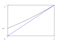
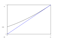
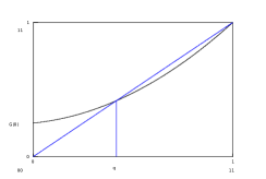
Figure 2. Generating function in the sub-critical (left), critical (middle) and super-critical (right) cases.

Using the branching property, we get:

$${\mathbb{P}}({\mathcal{E}}) ={\mathbb{P}}({\mathcal{E}}(\tau))$$

$$=\sum_{k\in{\mathbb{N}}}{\mathbb{P}}\bigl{(}{\mathcal{E}}\bigl{(}{\mathcal{S}}_{1}(\tau)\bigr{)},\ldots,{\mathcal{E}}\bigl{(}{\mathcal{S}}_{k}(\tau)\bigr{)}\bigm{|}k_{\varrho}(\tau)=k\bigr{)}p(k)$$

$$=\sum_{k\in{\mathbb{N}}}{\mathbb{P}}({\mathcal{E}})^{k}p(k)$$

$$=g\bigl{(}{\mathbb{P}}({\mathcal{E}})\bigr{)}.$$

We deduce that ${\mathbb{P}}({\mathcal{E}})$ is a root in $[0,1]$ of the equation $g(r)=r$. The following corollary is then an immediate consequence of Remark 2.4.

Corollary 2.5.

For a critical or sub-critical GW tree with offspring distribution $p$ satisfying (13), we have a.s. extinction, that is ${\mathbb{P}}({\mathcal{E}})=1$.

Let $p$ be a super-critical offspring distribution satisfying (13). In this case we have $0<q<1$, and thus ${\mathbb{P}}({\mathcal{E}})>0$. For $n\in{\mathbb{N}}$, we set:

(14) $$\tilde{p}(n)=q^{n-1}p(n).$$

Since $\sum_{n\in{\mathbb{N}}}\tilde{p}(n)={g(q)}/{q}=1$, we deduce that $\tilde{p}=(\tilde{p}(n),n\in{\mathbb{N}})$ is a probability distribution on ${\mathbb{N}}$. Since $g_{\tilde{p}}(r)=g(qr)/q$, we deduce that $g_{\tilde{p}}^{\prime}(1)=g^{\prime}(q)<1$. This implies that the offspring distribution $\tilde{p}$ is sub-critical. Notice that $\tilde{p}$ satisfies (13). In particular, if $\tilde{\tau}$ is a GW tree with offspring distribution $\tilde{p}$, we have ${\mathbb{P}}({\mathcal{E}}(\tilde{\tau}))=1$.

Lemma 2.6.

For a super-critical GW tree $\tau$ with offspring distribution $p$ satisfying (13), we have ${\mathbb{P}}({\mathcal{E}})=q$. Furthermore, conditionally on the extinction event, $\tau$ is distributed as a sub-critical GW tree $\tilde{\tau}$ with offspring distribution $\tilde{p}$ given by (14).

Proof.

According to Corollary 2.5, a.s. $\tilde{\tau}$ belongs to ${\mathbb{T}}_{0}$. For ${\mathbf{t}}\in{\mathbb{T}}_{0}$, we have:

$$q{\mathbb{P}}(\tilde{\tau}={\mathbf{t}})=q\prod_{u\in{\mathbf{t}}}p(k_{u}({\mathbf{t}}))q^{k_{u}({\mathbf{t}})-1}\\ =q^{1+\sum_{u\in{\mathbf{t}}}(k_{u}({\mathbf{t}})-1)}\prod_{u\in{\mathbf{t}}}p(k_{u}({\mathbf{t}}))={\mathbb{P}}(\tau={\mathbf{t}}),$$

where we used (12) and the definition of $\tilde{p}$ for the first equality and (4) as well as (12) for the last one. We deduce, by summing the previous equality over all finite trees ${\mathbf{t}}\in{\mathbb{T}}_{0}$ that, for any non-negative function ${\mathcal{H}}$ defined on ${\mathbb{T}}_{0}$,

$${\mathbb{E}}\left[{\mathcal{H}}(\tau){\bf 1}_{\{\tau\in{\mathbb{T}}_{0}\}}\right]=q{\mathbb{E}}\left[{\mathcal{H}}(\tilde{\tau})\right],$$

as a.s. $\tilde{\tau}$ is finite. Taking ${\mathcal{H}}=1$, we deduce that ${\mathbb{P}}({\mathcal{E}}(\tau))=q$. Then we get:

$${\mathbb{E}}\left[{\mathcal{H}}(\tau)|{\mathcal{E}}(\tau)\right]={\mathbb{E}}\left[{\mathcal{H}}(\tilde{\tau})\right].$$

Thus, conditionally on the extinction event, $\tau$ is distributed as $\tilde{\tau}$. ∎

We deduce the following corollary on GW processes.

Corollary 2.7.

Let $Z$ be a super-critical GW process with offspring distribution $p$ satisfying (13). Conditionally on the extinction event, $Z$ is distributed as a sub-critical GW process $\tilde{Z}$ with offspring distribution $\tilde{p}$ given by (14).

2.2.3. Distribution of the super-critical GW tree cond. on non-extinction

Let $\tau$ be a super-critical GW tree with offspring distribution $p$ satisfying (13). We shall present a decomposition of the super-critical GW tree conditionally on the non-extinction event ${\mathcal{E}}^{c}=\{H(\tau)=+\infty\}$. Notice that the event ${\mathcal{E}}^{c}$ has positive probability $1-q$, with $q$ the smallest root of $g(r)=r$ on $[0,1]$.

We say that $v\in{\mathbf{t}}$ is a survivor in ${\mathbf{t}}\in{\mathbb{T}}$ if ${\rm Card}\;(\{u\in{\mathbf{t}};\,v\prec u\})=+\infty$ and becomes extinct otherwise. We define the survivor process $(z_{h}^{s}({\mathbf{t}}),h\in{\mathbb{N}})$ by:

$$z_{h}^{s}({\mathbf{t}})={\rm Card}\;\bigl{(}\{u\in{\mathbf{t}};\,|u|=h\text{ and $u$ is a survivor}\}\bigr{)}.$$

Notice that the root ${\varrho}$ of $\tau$ is a survivor with probability $1-q$. Let $S$ and $E$ denote respectively the numbers of children of the root which are survivors and which become extinct. We define for $r,\ell\in[0,1]$:

$$G(r,\ell)={\mathbb{E}}\left[r^{S}\ell^{E}|{\mathcal{E}}^{c}\right].$$

We have the following lemma.

Lemma 2.8.

Let $\tau$ be a super-critical GW tree with offspring distribution $p$ satisfying (13) and let $q$ be the smallest root of $g(r)=r$ on $[0,1]$. We have for $r,\ell\in[0,1]$:

(15) $$G(r,\ell)=\frac{g\bigl{(}(1-q)r+q\ell\bigr{)}-g(q\ell)}{1-q}\cdot$$

Proof.

We have:

$${\mathbb{E}}\left[r^{S}\ell^{E}|{\mathcal{E}}^{c}\right] =\mathop{\frac{1}{1-q}}\nolimits{\mathbb{E}}\left[r^{S}\ell^{E}{\bf 1}_{\{S\geq 1\}}\right]$$

$$=\mathop{\frac{1}{1-q}}\nolimits\sum_{n\in{\mathbb{N}}^{*}}p(n)\sum_{k=1}^{n}\binom{n}{k}(1-q)^{k}r^{k}q^{n-k}\ell^{n-k}$$

$$=\mathop{\frac{1}{1-q}}\nolimits\sum_{n\in{\mathbb{N}}^{*}}p(n)\Bigl{(}\bigl{(}(1-q)r+q\ell\bigr{)}^{n}-(q\ell)^{n}\Bigr{)}$$

$$=\frac{g\bigl{(}(1-q)r+q\ell\bigr{)}-g(q\ell)}{1-q},$$

where we used the branching property and the fact that a GW tree with offspring distribution $p$ is finite with probability $q$ in the second equality. ∎

We consider the following multi-type GW tree $\hat{\tau}^{s}$ distributed as follows:

• Individuals are of type $s$ or of type $e$.

• The root of $\hat{\tau}^{s}$ is of type $s$.

• An individual of type $e$ produces only individuals of type $e$ according to the sub-critical offspring distribution $\tilde{p}$ defined by (14).

• An individual of type $s$ produces $S\geq 1$ individuals of type $s$ and $E$ of type $e$, with generating function ${\mathbb{E}}\left[r^{S}\ell^{E}\right]=G(r,\ell)$ given by (15). Furthermore the order of the $S$ individuals of type $s$ and of the $E$ individuals of type $e$ is uniform among the $\binom{E+S}{S}$ possible configurations. Thus the probability for an individual $u$ of type $s$ to have $n$ children and whose children of type $s$ are $\{ui,\,i\in A\}$, with $A$ a non-empty subset $\{1,\ldots,n\}$ of cardinal $|A|$, is:

  (16) $$p(n)(1-q)^{|A|-1}q^{n-|A|}.$$

  This indeed define a probability measure as:

  $$\sum_{n\in{\mathbb{N}}^{*}}\sum_{A\subset\{1,\ldots,n\},\,A\neq\emptyset} p(n)(1-q)^{|A|-1}q^{n-|A|}$$

  $$=\sum_{n\in{\mathbb{N}}^{*}}\sum_{k=1}^{n}p(n)\binom{n}{k}(1-q)^{k-1}q^{n-k}$$

  $$=\sum_{n\in{\mathbb{N}}^{*}}p(n)\frac{1-q^{n}}{1-q}$$

  $$=\frac{g(1)-g(q)}{1-q}=1.$$

Notice that an individual in $\hat{\tau}^{s}$ is a survivor if and only if it is of type $s$. We write $\tau^{s}$ for the ${\mathbb{T}}$-valued random variable defined as $\hat{\tau}^{s}$ when forgetting the types.

Using the branching property, it is easy to deduce the following corollary.

Corollary 2.9.

Let $\tau$ be a super-critical GW tree with offspring distribution $p$ satisfying (13). Conditionally on ${\mathcal{E}}^{c}$, $\tau$ is distributed as $\tau^{s}$.

Proof.

We denote by ${\mathcal{S}}_{h}=\{u\in\tau^{s},\,|u|=h\text{ and the type of $u$ is $s$}\}$ the set of individuals of $\tau^{s}$ at height $h$ of type $s$. Because ancestors of an individual of type $s$ are also of type $s$ and that every individual of type $s$ has at least a child of type $s$, we deduce that $\hat{\tau}^{s}$ truncated at level $h$ is characterized by $r_{h}(\tau^{s})$ and ${\mathcal{S}}_{h}$.

Let ${\mathbf{t}}\in{\mathbb{T}}_{0}$ such that $H({\mathbf{t}})=h$ and $A\subset\{u\in{\mathbf{t}},\,|u|=h\}$ with $A\neq\emptyset$. Set $n=z_{h}({\mathbf{t}})$. Let ${\mathcal{A}}=\bigcup_{u\in A}A_{u}$ be the set of ancestors of $A$ and set ${\mathcal{A}}^{c}=r_{h-1}({\mathbf{t}})\backslash{\mathcal{A}}$. For $u\in{\mathcal{A}}$, we denote by $k_{u}^{s}({\mathbf{t}},A)$ the number of children of $u$ in ${\mathbf{t}}$ that belong to ${\mathcal{A}}\cup A$. We have:

$${\mathbb{P}}(r_{h}(\tau^{s}) ={\mathbf{t}},\,{\mathcal{S}}_{h}=A)$$

$$=\prod_{u\in{\mathcal{A}}^{c}}\tilde{p}(k_{u}({\mathbf{t}}))\prod_{u\in{\mathcal{A}}}p(k_{u}({\mathbf{t}}))\,(1-q)^{k_{u}^{s}({\mathbf{t}},A)-1}q^{k_{u}({\mathbf{t}})-k_{u}^{s}({\mathbf{t}},A)}$$

$$=\left(\prod_{u\in{\mathcal{A}}^{c}\cup{\mathcal{A}}}p(k_{u}({\mathbf{t}}))\right)\,\left(\frac{1-q}{q}\right)^{\sum_{u\in{\mathcal{A}}}(k_{u}^{s}({\mathbf{t}},A)-1)}\,q^{\sum_{u\in{\mathcal{A}}\cup{\mathcal{A}}^{c}}(k_{u}({\mathbf{t}})-1)}$$

$$={\mathbb{P}}(r_{h}(\tau)={\mathbf{t}})\,\left(\frac{1-q}{q}\right)^{|A|-1}\,q^{n-1}$$

$$=\mathop{\frac{1}{1-q}}\nolimits\,{\mathbb{P}}(r_{h}(\tau)={\mathbf{t}})\,(1-q)^{|A|}q^{n-|A|},$$

where we used (16) for the first equality and, for the third equality, formula (4) twice as well as $n=z_{h}({\mathbf{t}})$. Summing the previous equality over all possible choices for $A$, we get (recall that $A$ is non empty):

$${\mathbb{P}}(r_{h}(\tau^{s})={\mathbf{t}}) =\sum_{A}\mathop{\frac{1}{1-q}}\nolimits\,{\mathbb{P}}(r_{h}(\tau)={\mathbf{t}})\,(1-q)^{|A|}q^{n-|A|}$$

$$=\mathop{\frac{1}{1-q}}\nolimits\,{\mathbb{P}}(r_{h}(\tau)={\mathbf{t}})\sum_{k=1}^{n}\binom{n}{k}\,(1-q)^{k}q^{n-k}$$

$$={\mathbb{P}}(r_{h}(\tau)={\mathbf{t}})\,\frac{1-q^{n}}{1-q}\cdot$$

On the other hand, we have:

$${\mathbb{P}}(r_{h}(\tau)={\mathbf{t}}|\,{\mathcal{E}}^{c})=\frac{{\mathbb{P}}(r_{h}(\tau)={\mathbf{t}})-{\mathbb{P}}(r_{h}(\tau)={\mathbf{t}},{\mathcal{E}})}{1-{\mathbb{P}}({\mathcal{E}})}\\ =\frac{{\mathbb{P}}(r_{h}(\tau)={\mathbf{t}})-{\mathbb{P}}(r_{h}(\tau)={\mathbf{t}})\,q^{n}}{1-q}={\mathbb{P}}(r_{h}(\tau)={\mathbf{t}})\,\frac{1-q^{n}}{1-q},$$

where we used the branching property at height $h$ for $\tau$ for the second equality. Thus we have obtained that ${\mathbb{P}}(r_{h}(\tau^{s})={\mathbf{t}})={\mathbb{P}}(r_{h}(\tau)={\mathbf{t}}|\,{\mathcal{E}}^{c})$ for all ${\mathbf{t}}\in{\mathbb{T}}_{0}$, which concludes the proof. ∎

In particular, it is easy to deduce from the definition of $\tau^{s}$, that the backbone process $(z_{h}^{s}(\tau),h\in{\mathbb{N}})$ is conditionally on ${\mathcal{E}}^{c}$ a GW process whose offspring distribution $\hat{p}$ has generating function:

$$g_{\hat{p}}(r)=G(r,1)=\frac{g((1-q)r+q)-q}{1-q}\cdot$$

The mean of $\hat{p}$ is $g_{\hat{p}}^{\prime}(1)=g^{\prime}(1)$ the mean of $p$. Notice also that $\hat{p}(0)=0$, so that the GW process with offspring distribution $\hat{p}$ is super-critical and a.s. does not suffer extinction.

Recall that the GW tree $\tau$ conditionally on the extinction event is a GW tree with offspring distribution $\tilde{p}$, whose generating function is:

$$g_{\tilde{p}}(r)=\frac{g(qr)}{q}\cdot$$

We observe that the generating function $g(r)$ of the super-critical offspring distribution $p$ can be recovered from the extinction probability $q$, the generating functions $g_{\hat{p}}$ and $g_{\tilde{p}}$ of the offspring distribution of the backbone process (for $r\geq q$) and of the GW tree conditionally on the extinction event (for $r\leq q$):

$$g(r)=qg_{\tilde{p}}\left(\frac{r}{q}\right){\bf 1}_{[0,q]}(r)+\left(q+(1-q)g_{\hat{p}}\left(\frac{r-q}{1-q}\right)\right){\bf 1}_{(q,1]}(r).$$

We can therefore read from the super-critical generating functions $g_{p}$, the sub-critical generating function $g_{\tilde{p}}$ and the super-critical generating function $g_{\hat{p}}$, see Figure 3.

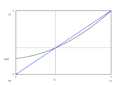
Figure 3. The generating functions $g_{p}$, $g_{\tilde{p}}$ in the lower sub-square and $g_{\hat{p}}$ in the upper sub-square (up to a scaling factor).

2.3. Kesten’s tree

2.3.1. Definition

We define what we call Kesten’s tree which is a multi-type Galton-Watson tree, that is a random tree where all individuals reproduce independently of the others, but the offspring distrbution depends on the type of the individual. For a probability distribution $p=(p(n),n\in{\mathbb{N}})$ on ${\mathbb{N}}$ with finite mean $m$, the corresponding size-biased distribution $p^{*}=(p^{*}(n),n\in{\mathbb{N}})$ is defined by:

$$p^{*}(n)=\frac{np(n)}{m}\cdot$$

Definition 2.10.

Let $p$ be an offspring distribution satisfying (13) with finite mean ($m<+\infty$). Kesten’s tree associated with the probability distribution $p$ on ${\mathbb{N}}$ is a multi-type GW tree $\hat{\tau}^{*}$ distributed as follows:

• Individuals are normal or special.

• The root of $\hat{\tau}^{*}$ is special.

• A normal individual produces only normal individuals according to $p$.

• A special individual produces individuals according to the size-biased distribution $p^{*}$ (notice that it always has at least one offspring since $p^{*}(0)=0$). One of them, chosen uniformly at random, is special, the others (if any) are normal.

We write $\tau^{*}$ for the ${\mathbb{T}}$-valued random variable defined as $\hat{\tau}^{*}$ when forgetting the types. Notice $\tau^{*}$ belongs a.s. to ${\mathbb{T}}_{1}$ if $p$ is sub-critical or critical. In the next lemma we provide a link between the distribution of $\tau$ and of $\tau^{*}$.

Lemma 2.11.

Let $p$ be an offspring distribution satisfying (13) with finite mean ($m<+\infty$), $\tau$ be a GW tree with offspring distribution $p$ and let $\tau^{*}$ be Kesten’s tree associated with $p$. For all $n\in{\mathbb{N}}$, ${\mathbf{t}}\in{\mathbb{T}}_{0}$ and $v\in{\mathbf{t}}$ such that $H({\mathbf{t}})=|v|=n$, we have:

$${\mathbb{P}}\left(r_{n}(\tau^{*})={\mathbf{t}},\text{$v$ is special}\right) =\mathop{\frac{1}{m^{n}}}\nolimits{\mathbb{P}}\left(r_{n}(\tau)={\mathbf{t}}\right),$$

(17) $${\mathbb{P}}\left(r_{n}(\tau^{*})={\mathbf{t}}\right) =\frac{z_{n}({\mathbf{t}})}{m^{n}}{\mathbb{P}}\left(r_{n}(\tau)={\mathbf{t}}\right).$$

Proof.

Notice that if $u$ is special, then the probability that it has $k_{u}$ children and $ui$ is special (with $i$ given and $1\leq i\leq k_{u}$) is just $p(k_{u})/m$. Let $n\in{\mathbb{N}}$, ${\mathbf{t}}\in{\mathbb{T}}^{(n)}$ and $v\in{\mathbf{t}}$ such that $H({\mathbf{t}})=|v|=n$. Using (11), we have:

$${\mathbb{P}}\left(r_{n}(\tau^{*})={\mathbf{t}},\text{ $v$ is special}\right)=\prod_{u\in{\mathbf{t}}\setminus{\rm A}_{v},\,|u|<n}p(k_{u}({\mathbf{t}}))\prod_{u\in{\rm A}_{v}}\frac{p(k_{u}({\mathbf{t}}))}{m}\\ =\mathop{\frac{1}{m^{n}}}\nolimits{\mathbb{P}}\left(r_{n}(\tau)={\mathbf{t}}\right).$$

Since there is only one special element of ${\mathbf{t}}$ at level $n$ among the $z_{n}({\mathbf{t}})$ elements of ${\mathbf{t}}$ at level $n$, we obtain (17). ∎

We consider the renormalized GW process $(W_{n},n\in{\mathbb{N}})$ defined by:

(18) $$W_{n}=\frac{z_{n}(\tau)}{m^{n}}\cdot$$

Notice that $W_{0}=1$. If necessary, we shall write $W_{n}({\mathbf{t}})=z_{n}({\mathbf{t}})/m^{n}$ to denote the dependence in ${\mathbf{t}}$. We consider the filtration ${\mathcal{F}}=({\mathcal{F}}_{n},n\in{\mathbb{N}})$ generated by $\tau$: ${\mathcal{F}}_{n}=\sigma(r_{n}(\tau))$.

Corollary 2.12.

Let $p$ be an offspring distribution satisfying (13) with finite mean ($m<+\infty$). The process $(W_{n},n\in{\mathbb{N}})$ is a non-negative martingale adapted to the filtration ${\mathcal{F}}$.

Proof.

Let ${\rm P}$ and ${\rm P}^{*}$ denote respectively the distribution on ${\mathbb{T}}$ of a GW tree $\tau$ with offspring distribution $p$ and Kesten’s tree $\tau^{*}$ associated with $p$. We deduce from Lemma 2.11 that for all $n\geq 0$:

(19) $$d{\rm P}^{*}_{|{\mathcal{F}}_{n}}({\mathbf{t}})=W_{n}({\mathbf{t}})\,d{\rm P}_{|{\mathcal{F}}_{n}}({\mathbf{t}}).$$

This implies that $(W_{n},n\geq 0)$ is a non-negative ${\rm P}$-martingale adapted to the filtration ${\mathcal{F}}$. ∎

2.3.2. Asymptotic equivalence of the GW process in the super-critical case

Let $\tau$ be a super-critical GW tree with offspring distribution $p$ satisfying (13). Let $m=g^{\prime}(1)$ be the mean of $p$. Recall the renormalized GW process $(W_{n},n\in{\mathbb{N}})$ defined by (18). If necessary, we shall write $W_{n}(\tau)$ to denote the dependence on $\tau$.

Lemma 2.13.

Let $p$ be a super-critical offspring distribution satisfying (13) with finite mean ($m<+\infty$). The sequence $(W_{n},n\in{\mathbb{N}})$ converges a.s. to a random variable $W$ s.t. ${\mathbb{E}}[W]\leq 1$ and ${\mathbb{P}}(W=0)\in\{q,1\}$.

Proof.

According to Corollary 2.12, $(W_{n},n\in{\mathbb{N}})$ is a non-negative martingale. Thanks to the convergence theorem for martingales, see Theorem 4.2.10 in [18], we get that it converges a.s. to a non-negative random variable $W$ such that ${\mathbb{E}}[W]\leq 1$.

By decomposing $\tau$ with respect to the children of the root, we get:

$$W_{n}(\tau)=\mathop{\frac{1}{m}}\nolimits\sum_{i=1}^{k_{\varrho}(\tau)}W_{n-1}({\mathcal{S}}_{i}(\tau)).$$

The branching property implies that conditionally on $k_{\varrho}(\tau)$, the random trees ${\mathcal{S}}_{i}(\tau)$, $1\leq i\leq k_{\varrho}(\tau)$ are independent and distributed as $\tau$. In particular, $(W_{n}({\mathcal{S}}_{i}(\tau)),n\in{\mathbb{N}})$ converges a.s. to a limit, say $W^{i}$, where $(W^{i},i\in{\mathbb{N}}^{*})$ are independent non-negative random variables distributed as $W$ and independent of $k_{\varrho}(\tau)$. By taking the limit as $n$ goes to infinity, we deduce that a.s.:

$$W=\mathop{\frac{1}{m}}\nolimits\sum_{i=1}^{k_{\varrho}(\tau)}W^{i}.$$

This implies that:

$${\mathbb{P}}(W=0)=\sum_{n\in{\mathbb{N}}}p(n){\mathbb{P}}(W^{1}=0,\ldots,W^{n}=0)=g({\mathbb{P}}(W=0)).$$

This implies that ${\mathbb{P}}(W=0)$ is a non-negative solution of $g(r)=r$ and so belongs to $\{q,1\}$. ∎

Remark 2.14.

Assume that ${\mathbb{P}}(W=0)=q$. Since ${\mathcal{E}}\subset\{W=0\}$ and ${\mathbb{P}}({\mathcal{E}})=q$, we deduce that on the survival event ${\mathcal{E}}^{c}$ a.s. $\lim_{n\rightarrow+\infty}\frac{z_{n}(\tau)}{m^{n}}=W>0$. (On the extinction event ${\mathcal{E}}$, we have that a.s. $z_{n}(\tau)=0$ for $n$ large.) So, a.s. on the survival event, the population size at level $n$ behaves like a positive finite random constant times $m^{n}$.

We aim to compute ${\mathbb{P}}(W=0)$. The following result goes back to Kesten and Stigum [31] and we present the proof of Lyons, Pemantle and Peres [33]. Recall that $\zeta$ is a random variable with distribution $p$. We use the notation $\log^{+}(r)=\max(\log(r),0)$.

Theorem 2.15.

Let $p$ be a super-critical offspring distribution satisfying (13) with finite mean ($m<+\infty$). Then we have:

• ${\mathbb{P}}(W=0)=q$ if ${\mathbb{E}}\left[\zeta\log^{+}(\zeta)\right]<+\infty$.

• ${\mathbb{P}}(W=0)=1$ if ${\mathbb{E}}\left[\zeta\log^{+}(\zeta)\right]=+\infty$.

Proof.

We use notations from the proof of Corollary 2.12: ${\rm P}$ and ${\rm P}^{*}$ denote respectively the distribution of a GW tree $\tau$ with offspring distribution $p$ and of Kesten’s tree $\tau^{*}$ associated with $p$. According to (19), for all $n\geq 0$:

$$d{\rm P}^{*}_{|{\mathcal{F}}_{n}}=W_{n}\,d{\rm P}_{|{\mathcal{F}}_{n}}.$$

This implies that $(W_{n},n\geq 0)$ converges ${\rm P}$-a.s. (this is already in Lemma 2.13) and ${\rm P}^{*}$-a.s. to $W$ taking values in $[0,+\infty]$. According to Theorem 4.3.3 in [18], we get that for any measurable subset $B$ of ${\mathbb{T}}$:

$${\rm P}^{*}(B)={\rm E}[W{\bf 1}_{B}]+{\rm P}^{*}(B,W=+\infty).$$

Taking $B=\Omega$ in the previous equality gives:

(20) $$\begin{cases}{\rm E}[W]=1\Leftrightarrow{\rm P}^{*}(W=+\infty)=0\quad\text{and}\\ {\rm P}(W=0)=1\Leftrightarrow{\rm P}^{*}(W=+\infty)=1.\end{cases}$$

So we shall study the behavior of $W$ under ${\rm P}^{*}$, which turns out to be (almost) elementary. We first use a similar description as (1) to describe $(z_{n}(\tau^{*}),n\in{\mathbb{N}})$.

Recall that $\zeta$ is a random variable with distribution $p$. Notice that $p^{*}(0)=0$, and let $Y$ be a random variable such that $Y+1$ has distribution $p^{*}$. Let $(\zeta_{i,n};i\in{\mathbb{N}},n\in{\mathbb{N}})$ be independent random variables distributed as $\zeta$. Let $(Y_{n},n\in{\mathbb{N}}^{*})$ be independent random variables distributed as $Y$ and independent of $(\zeta_{i,n};i\in{\mathbb{N}},n\in{\mathbb{N}})$. We set $Z^{*}_{0}=0$ and for $n\in{\mathbb{N}}^{*}$:

$$Z^{*}_{n}=Y_{n}+\sum_{i=1}^{Z^{*}_{n-1}}\zeta_{i,n},$$

with the convention that $\sum_{\emptyset}=0$. In particular $(Z_{n}^{*},n\in{\mathbb{N}})$ is a GW process with offspring distribution $p$ and immigration distributed as $Y$. By construction $(Z_{n}^{*}+1,n\in{\mathbb{N}})$ is distributed as $(z_{n}(\tau^{*}),n\in{\mathbb{N}})$. We deduce that $(W_{n},n\in{\mathbb{N}})$ is under ${\rm P}^{*}$ distributed as $(W^{*}_{n}+m^{-n},n\in{\mathbb{N}})$, with $W^{*}_{n}=Z^{*}_{n}/m^{n}$.

We recall the following result, which can be deduced from the Borel-Cantelli lemma. Let $(X_{n},n\in{\mathbb{N}})$ be random variables distributed as a non-negative random variable $X$. We have:

(21) $${\mathbb{E}}[X]<+\infty\Rightarrow\text{ a.s. }\lim_{n\rightarrow+\infty}\frac{X_{n}}{n}=0.$$

Furthermore, if the random variables $(X_{n},n\in{\mathbb{N}})$ are independent, then:

(22) $${\mathbb{E}}[X]=+\infty\Rightarrow\text{ a.s. }\limsup_{n\rightarrow+\infty}\frac{X_{n}}{n}=+\infty.$$

We consider the case: ${\mathbb{E}}\left[\zeta\log^{+}(\zeta)\right]<+\infty$. This implies that ${\mathbb{E}}[\log^{+}(Y)]<+\infty$. And according to (21), we deduce that for $\varepsilon>0$, ${\rm P}^{*}$-a.s. $Y_{n}\leq\mathop{\mathrm{e}^{n\varepsilon}}$ for $n$ large enough. Denote by ${\mathcal{Y}}$ the $\sigma$-field generated by $(Y_{n},n\in{\mathbb{N}}^{*})$ and by $({\mathcal{F}}^{*}_{n},n\in{\mathbb{N}})$ the filtration generated by $(W^{*}_{n},n\in{\mathbb{N}})$. Using the branching property, it is easy to get:

$${\mathbb{E}}\left[W^{*}_{n}|{\mathcal{Y}},{\mathcal{F}}^{*}_{n-1}\right]=\mathop{\frac{1}{m^{n}}}\nolimits{\mathbb{E}}\left[Z^{*}_{n}|{\mathcal{Y}},{\mathcal{F}}^{*}_{n-1}\right]=\frac{Z^{*}_{n-1}}{m^{n-1}}+\frac{Y_{n}}{m^{n}}\geq W^{*}_{n-1}.$$

We deduce that $(W^{*}_{n},n\in{\mathbb{N}})$ is a non-negative sub-martingale with respect to ${\mathbb{P}}(\cdot|{\mathcal{Y}})$. We also obtain:

$${\mathbb{E}}\left[W^{*}_{n}|{\mathcal{Y}}\right]=\sum_{k=1}^{n}\frac{Y_{k}}{m^{k}}\leq\sum_{k=1}^{+\infty}\frac{Y_{k}}{m^{k}}\cdot$$

For $\varepsilon>0$, we have that ${\mathbb{P}}$-a.s. $Y_{n}\leq\mathop{\mathrm{e}^{n\varepsilon}}$ for $n$ large enough. We deduce that ${\mathbb{P}}$-a.s. we have $\sup_{n\in{\mathbb{N}}}{\mathbb{E}}\left[W^{*}_{n}|{\mathcal{Y}}\right]<+\infty$. Since the non-negative sub-martingale $(W^{*}_{n},n\in{\mathbb{N}})$ is bounded in $L^{1}({\mathbb{P}}(\cdot|{\mathcal{Y}}))$, we get that it converges ${\mathbb{P}}(\cdot|{\mathcal{Y}})$-a.s. to a finite limit. Since $(W^{*}_{n}+m^{-n},n\in{\mathbb{N}})$ is distributed as $(W_{n},n\in{\mathbb{N}})$ under ${\rm P}^{*}$, we get that ${\rm P}^{*}$-a.s. $W$ is finite. Use the first part of (20) to deduce that ${\rm E}[W]=1$. Since ${\rm P}(W=0)\in\{q,1\}$, see Lemma 2.13, we get that ${\rm P}(W=0)=q$.

We consider the case: ${\mathbb{E}}\left[\zeta\log^{+}(\zeta)\right]=+\infty$. According to (22), we deduce that for any $\varepsilon>0$, a.s. $Y_{n}\geq\mathop{\mathrm{e}^{n/\varepsilon}}$ for infinitely many $n$. Since $Z_{n}^{*}\geq Y_{n}$ and $(W^{*}_{n}+m^{-n},n\in{\mathbb{N}})$ is distributed as $(W_{n},n\in{\mathbb{N}})$ under ${\rm P}^{*}$, we deduce that ${\rm P}^{*}$-a.s. $W_{n}\geq\mathop{\mathrm{e}^{n(-\log(m)+1/\varepsilon)}}$ for infinitely many $n$. Since the sequence $(W_{n},n\in{\mathbb{N}})$ converges ${\rm P}^{*}$-a.s. to $W$ taking values in $[0,+\infty]$, we deduce, by taking $\varepsilon>0$ small enough that ${\rm P}^{*}$-a.s. $W=+\infty$. Use the second part of (20) to deduce that ${\rm P}$-a.s.$W=0$. ∎

3. Local limits of Galton-Watson trees

There are many kinds of limits that can be considered in order to study large trees, among them are the local limits and the scaling limits. The local limits look at the trees up to an arbitrary fixed height and therefore only sees what happen at a finite distance from the root. Scaling limits consider sequences of trees where the branches are scaled by some factor so that all the nodes remain at finite distance from the root. These scaling limits, which lead to the so-called continuum random trees where the branches have infinitesimal length, have been intensively studied in recent years, see [8, 16, 17].

We will focus in this lecture only on local limits of critical or sub-critical GW trees conditioned on being large. The most famous type of such a conditioning is Kesten’s theorem which states that critical or sub-critical GW trees conditioned on reaching large heights converge to Kesten’s tree which is a (multi-type) GW tree with a unique infinite spine. This result is recalled in Theorem 3.1. In order to consider other conditionings, we shall give in Section 3.1, see Proposition 3.3, an elementary characterization of the local convergence which is the key ingredient of the method presented here.

All the conditionings we shall consider can be stated in terms of a functional $A({\mathbf{t}})$ of the tree ${\mathbf{t}}$ and the events we condition on are either of the form $\{A(\tau)\geq n\}$ or $\{A(\tau)=n\}$, with $n$ large. In Section 3.2, we give general assumptions on $A$ so that a critical GW tree conditioned on such an event converges as $n$ goes to infinity, in distribution to Kesten’s tree, see our main result, Theorem 3.7.

We then apply this result in Section 3.3 by considering, in the critical case, the following functional: the height of the tree (recovering Kesten’s theorem) in Section 3.3.1; the total progeny of the tree in Section 3.3.5; or the total number of leaves in Section 3.3.6. Those limits where already known, but under stronger hypothesis on the offspring distribution (higher moments or tail conditions), whereas we stress out that no further assumption are needed in the critical case than the non-degeneracy condition (13). Other new results can also very simply be derived in the critical case such as: the number of nodes with given out-degree, which include all the previous results, in Section 3.3.7; the maximal out-degree in Section 3.3.2; the Horton-Strahler number in Section 3.3.3 or the size of the largest generation in Section 3.3.4. See also Section 3.3.8 for further extensions. The result can also be extended to sub-critical GW trees but only when $A$ is the height of the tree. Most of this material is extracted from [4] completed with some recent results from [25, 24].

The sub-critical case is more involved and we only present here some results in Section 3.4 without any proofs. All the proofs can be found in [3]. In the sub-critical case, when conditioning on the number of nodes with given out-degree, two cases may appear. In the so-called generic case presented in Section 3.4.2, the limiting tree is still Kesten’s tree but with a modified offspring distribution, see Proposition 3.32. In the non-generic case, Section 3.4.3, a condensation phenomenon occurs: a node that stays at a bounded distance from the root has more and more offsprings as $n$ goes to infinity; and in the limit, the tree has a (unique) node with infinitely many offsprings, see Proposition 3.35. This phenomenon has first been pointed out in [27] and in [26] when conditioning on the total progeny. We end this chapter by giving in Section 3.4.4 a characterization of generic and non-generic offspring distributions, which provides non intuitive behavior (see Remark 3.38).

3.1. The topology of local convergence

3.1.1. Kesten’s theorem

We work on the set ${\mathbb{T}}$ of discrete trees with no infinite nodes, introduced in Section 2.1. Recall that ${\mathbb{T}}_{0}$, resp. ${\mathbb{T}}^{(h)}$, denotes the subset of ${\mathbb{T}}$ of finite trees, resp. of trees with height less than $h$, see (5) and (6). Recall that the restriction functions $r_{h}$ from ${\mathbb{T}}$ to ${\mathbb{T}}^{(h)}$ is defined in (9). When a sequence of random trees $(T_{n},{n\in{\mathbb{N}}})$ converges in distribution with respect to the distance $\delta$ (also called the local topology) toward a random tree $T$, we shall write:

(23) $$T_{n}\overset{(d)}{\longrightarrow}T.$$

According to (10), the fact that all the open balls are closed, and the Portmanteau theorem (see [12] Theorem 2.1), we deduce that if (23) then:

(24) $$\forall h\in{\mathbb{N}},\ \forall{\mathbf{t}}\in{\mathbb{T}}^{(h)},\quad\lim_{n\rightarrow+\infty}{\mathbb{P}}\bigl{(}r_{h}(T_{n})={\mathbf{t}}\bigr{)}={\mathbb{P}}\bigl{(}r_{h}(T)={\mathbf{t}}\bigr{)}.$$

Conversely, since $\delta$ is an ultra-metric, we get that the intersection of two balls is a ball (possibly empty). Thus the set of balls and the empty set is a $\pi$-system. We deduce from Theorem 2.3 in [12] that (24) implies (23). Thus (24) (23) are equivalent.

Convergence in distribution for the local topology appears in the following Kesten’s theorem. Recall that the distribution of Kesten’s tree is given in Definition 2.10.

Theorem 3.1 (Kesten [30]).

Let $p$ be a critical or sub-critical offspring distribution satisfying (13). Let $\tau$ be a GW tree with offspring distribution $p$ and $\tau^{*}$ be Kesten’s tree associated with $p$. For every non-negative integer $n$, let $\tau_{n}$ be a random tree distributed as $\tau$ conditionally on $\{H(\tau)\geq n\}$. Then we have:

$$\tau_{n}\overset{(d)}{\longrightarrow}\tau^{*}.$$

This theorem is stated in [30] with an additional second moment condition. The proof of the theorem stated as above is due to Janson [26]. We will give a proof of that theorem in Section 3.3.1 as an application of a more general result, see Theorem 3.7 in the critical case and Theorem 3.10 in the sub-critical case.

3.1.2. A characterization of the convergence in distribution

Recall that for a tree ${\mathbf{t}}\in{\mathbb{T}}$, we denote by ${\mathcal{L}}_{0}({\mathbf{t}})$ the set of its leaves. If ${\mathbf{t}}\in{\mathbb{T}}$ is a tree, $x\in{\mathcal{L}}_{0}({\mathbf{t}})$ is a leaf of the tree ${\mathbf{t}}$ and ${\mathbf{t}}^{\prime}\in{\mathbb{T}}$ is another tree, we denote by ${\mathbf{t}}\circledast_{x}{\mathbf{t}}^{\prime}$ the tree obtained by grafting the tree ${\mathbf{t}}^{\prime}$ on the leaf $x$ of the tree ${\mathbf{t}}$ i.e.

$${\mathbf{t}}\circledast_{x}{\mathbf{t}}^{\prime}={\mathbf{t}}\cup\{xu,u\in{\mathbf{t}}^{\prime}\}.$$

For every tree ${\mathbf{t}}\in{\mathbb{T}}$, and every leaf $x\in{\mathcal{L}}_{0}({\mathbf{t}})$ of ${\mathbf{t}}$, we denote by

$${\mathbb{T}}({\mathbf{t}},x)=\{{\mathbf{t}}\circledast_{x}{\mathbf{t}}^{\prime},\ {\mathbf{t}}^{\prime}\in{\mathbb{T}}\}$$

the set of all trees obtained by grafting some tree on the leaf $x$ of ${\mathbf{t}}$. Notice ${\mathbb{T}}({\mathbf{t}},x)$ is closed as $s\in{\mathbb{T}}({\mathbf{t}},x)$ if and only if $k_{u}(s)=k_{u}(t)$ for all $u\in{\mathbf{t}}\setminus\{x\}$. We shall see later that it is also open (see Lemma 3.6).

Computations of the probability of GW trees (or Kesten’s tree) to belong to such sets are very easy and lead to simple formulas. For example, we have for $\tau$ a GW tree with offspring distribution $p$, and all finite tree ${\mathbf{t}}\in{\mathbb{T}}_{0}$ and leaf $x\in{\mathcal{L}}_{0}({\mathbf{t}})$:

(25) $${\mathbb{P}}(\tau={\mathbf{t}})={\mathbb{P}}\bigl{(}\tau\in{\mathbb{T}}({\mathbf{t}},x),\ k_{x}(\tau)=0\bigr{)}={\mathbb{P}}\bigl{(}\tau\in{\mathbb{T}}({\mathbf{t}},x)\bigr{)}p(0).$$

The next lemma is another example of the simplicity of the formulas.

Lemma 3.2.

Let $p$ be an offspring distribution satisfying (13) with finite mean ($m<+\infty$). Let $\tau$ be a GW tree with offspring distribution $p$ and let $\tau^{*}$ be Kesten’s tree associated with $p$. Then we have, for all finite tree ${\mathbf{t}}\in{\mathbb{T}}_{0}$ and leaf $x\in{\mathcal{L}}_{0}({\mathbf{t}})$:

(26) $${\mathbb{P}}\bigl{(}\tau^{*}\in{\mathbb{T}}({\mathbf{t}},x)\bigr{)}=\mathop{\frac{1}{m^{|x|}}}\nolimits{\mathbb{P}}\bigl{(}\tau\in{\mathbb{T}}({\mathbf{t}},x)\bigr{)}.$$

In the particular case of a critical offspring distribution ($m=1$), we get for all ${\mathbf{t}}\in{\mathbb{T}}_{0}$ and $x\in{\mathcal{L}}_{0}({\mathbf{t}})$:

$${\mathbb{P}}(\tau^{*}\in{\mathbb{T}}({\mathbf{t}},x))={\mathbb{P}}(\tau\in{\mathbb{T}}({\mathbf{t}},x)).$$

However, we have ${\mathbb{P}}(\tau\in{\mathbb{T}}_{0})=1$ and ${\mathbb{P}}(\tau^{*}\in{\mathbb{T}}_{1})=1$, with ${\mathbb{T}}_{1}$ the set of trees that have one and only one infinite spine, see (8).

Proof.

Let ${\mathbf{t}}\in{\mathbb{T}}_{0}$ and $x\in{\mathcal{L}}_{0}({\mathbf{t}})$. If $\tau^{*}\in{\mathbb{T}}({\mathbf{t}},x)$, then the node $x$ must be a special node in $\tau^{*}$ as the tree ${\mathbf{t}}$ is finite whereas the tree $\tau^{*}$ is a.s. infinite. Therefore, using arguments similar to those used in the proof of Lemma 2.11, we have:

$${\mathbb{P}}\bigl{(}\tau^{*}\in{\mathbb{T}}({\mathbf{t}},x)\bigr{)}=\prod_{u\in{\mathbf{t}}\setminus({\rm A}_{x}\cup\{x\})}p(k_{u}({\mathbf{t}}))\prod_{u\in{\rm A}_{x}}\frac{p(k_{u}({\mathbf{t}}))}{m}\\ =\mathop{\frac{1}{m^{|x|}}}\nolimits{\mathbb{P}}\left(\tau\in{\mathbb{T}}({\mathbf{t}},x)\right).$$

∎

For convergence in distribution in the set ${\mathbb{T}}_{0}\cup{\mathbb{T}}_{1}$, we have the following key characterization, whose proof is given in Section 3.1.3.

Proposition 3.3.

Let $(T_{n},{n\in{\mathbb{N}}})$ and $T$ be random trees taking values in the set ${\mathbb{T}}_{0}\cup{\mathbb{T}}_{1}$. Then the sequence $(T_{n},{n\geq 0})$ converges in distribution (for the local topology) to $T$ if and only if the two following conditions hold:

• for every finite tree ${\mathbf{t}}\in{\mathbb{T}}_{0}$, $\lim_{n\rightarrow+\infty}{\mathbb{P}}(T_{n}={\mathbf{t}})={\mathbb{P}}(T={\mathbf{t}})$;

• for every ${\mathbf{t}}\in{\mathbb{T}}_{0}$ and every leaf $x\in{\mathcal{L}}_{0}({\mathbf{t}})$, $\liminf_{n\rightarrow+\infty}{\mathbb{P}}\bigl{(}T_{n}\in{\mathbb{T}}({\mathbf{t}},x)\bigr{)}\geq{\mathbb{P}}\bigl{(}T\in{\mathbb{T}}({\mathbf{t}},x)\bigr{)}$.

3.1.3. Proof of Proposition 3.3

We denote by ${\mathcal{F}}$ the subclass of Borel sets of ${\mathbb{T}}$:

$${\mathcal{F}}=\bigl{\{}\{{\mathbf{t}}\},\ {\mathbf{t}}\in{\mathbb{T}}_{0}\bigr{\}}\cup\bigl{\{}{\mathbb{T}}({\mathbf{t}},x),\ {\mathbf{t}}\in{\mathbb{T}}_{0},\ x\in{\mathcal{L}}_{0}({\mathbf{t}})\bigr{\}}\cup\{\emptyset\}.$$

Lemma 3.4.

The family ${\mathcal{F}}$ is a $\pi$-system.

Proof.

Recall that a non-empty family of sets is a $\pi$-system if it is stable under finite intersection. For every ${\mathbf{t}}_{1},{\mathbf{t}}_{2}\in{\mathbb{T}}_{0}$ and every $x_{1}\in{\mathcal{L}}_{0}({\mathbf{t}}_{1})$, $x_{2}\in{\mathcal{L}}_{0}({\mathbf{t}}_{2})$, we have, if ${\mathbb{T}}({\mathbf{t}}_{1},x_{1})\neq{\mathbb{T}}({\mathbf{t}}_{2},x_{2})$:

(27) $${\mathbb{T}}({\mathbf{t}}_{1},x_{1})\cap{\mathbb{T}}({\mathbf{t}}_{2},x_{2})=\begin{cases}{\mathbb{T}}({\mathbf{t}}_{1},x_{1})&\mbox{if }{\mathbf{t}}_{1}\in{\mathbb{T}}({\mathbf{t}}_{2},x_{2})\text{ and }x_{2}\prec x_{1},\\ {\mathbb{T}}({\mathbf{t}}_{2},x_{2})&\mbox{if }{\mathbf{t}}_{2}\in{\mathbb{T}}({\mathbf{t}}_{1},x_{1})\text{ and }x_{1}\prec x_{2},\\ \{{\mathbf{t}}_{1}\cup{\mathbf{t}}_{2}\}&\mbox{if }{\mathbf{t}}_{1}={\mathbf{t}}\circledast_{x_{2}}{{\mathbf{t}}^{\prime}_{1}},\ {\mathbf{t}}_{2}={\mathbf{t}}\circledast_{x_{1}}{{\mathbf{t}}^{\prime}_{2}}\\ &\mbox{ and }x_{1}\neq x_{2}\ (see\ Figure\ \ref{fig:mickey}),\\ \emptyset&\mbox{in the other cases.}\end{cases}$$

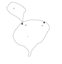
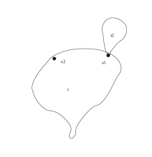
Figure 4. Exemple of the third case in (27). The trees are respectively ${\mathbf{t}}_{1}$, ${\mathbf{t}}_{2}$, ${\mathbf{t}}_{1}\cup{\mathbf{t}}_{2}$.

Thus ${\mathcal{F}}$ is stable under finite intersection, and is thus a $\pi$-system. ∎

Remark 3.5.

The third case in Equation (27) was ommited in the original paper [4] where only a special case was considered.

Lemma 3.6.

All the elements of ${\mathcal{F}}$ are open, and the family ${\mathcal{F}}$ restricted to ${\mathbb{T}}_{0}\cup{\mathbb{T}}_{1}$ is an open neighborhood system in ${\mathbb{T}}_{0}\cup{\mathbb{T}}_{1}$.

Proof.

We first check that all the elements of ${\mathcal{F}}$ are open. For ${\mathbf{t}}\in{\mathbb{T}}$ and $\varepsilon>0$, let $B({\mathbf{t}},\varepsilon)$ be the ball (which is open and closed) centered at ${\mathbf{t}}$ with radius $\varepsilon$. If ${\mathbf{t}}\in{\mathbb{T}}_{0}$, we have $\{{\mathbf{t}}\}=B({\mathbf{t}},2^{-h})$ for every $h>H({\mathbf{t}})$, thus $\{{\mathbf{t}}\}$ is open. Moreover, for every ${\mathbf{s}}\in{\mathbb{T}}({\mathbf{t}},x)$ for some $x\in{\mathcal{L}}_{0}({\mathbf{t}})$, we have

$$B\left({\mathbf{s}},2^{-H({\mathbf{t}})-1}\right)\subset{\mathbb{T}}({\mathbf{t}},x)$$

which proves that ${\mathbb{T}}({\mathbf{t}},x)$ is also open.

We check that ${\mathcal{F}}$ restricted to ${\mathbb{T}}_{0}\cup{\mathbb{T}}_{1}$ is a neighborhood system: that is, since all the elements of ${\mathcal{F}}$ are open, for all ${\mathbf{t}}\in{\mathbb{T}}_{0}\cup{\mathbb{T}}_{1}$ and $\varepsilon>0$, there exists an element of ${\mathcal{F}}$, say $A^{\prime}$, which is a subset of $B({\mathbf{t}},\varepsilon)$ and which contains ${\mathbf{t}}$.

If ${\mathbf{t}}\in{\mathbb{T}}_{0}$, it is enough to consider $A^{\prime}=\{{\mathbf{t}}\}$.

Let us suppose that ${\mathbf{t}}\in{\mathbb{T}}_{1}$. Let $(u_{n},n\in{\mathbb{N}}^{*})$ be the infinite spine of ${\mathbf{t}}$ so that $\bar{u}_{n}=u_{1}\ldots u_{n}\in{\mathbf{t}}$ for all $n\in{\mathbb{N}}^{*}$. Let $n\in{\mathbb{N}}^{*}$ such that $2^{-n}<\varepsilon$ and set ${\mathbf{t}}^{\prime}=\{v\in{\mathbf{t}};\,\bar{u}_{n}\not\in{\rm A}_{v}\}$. Notice that $\bar{u}_{n}\in{\mathbf{t}}^{\prime}$, and set $A^{\prime}={\mathbb{T}}({\mathbf{t}}^{\prime},\bar{u}_{n})$ so that $A^{\prime}$ belongs to the $\pi$-system ${\mathcal{F}}$. We get ${\mathbf{t}}\in A^{\prime}\subset B({\mathbf{t}},\varepsilon)$. ∎

We are now ready to prove Proposition 3.3, following ideas of the proof of Theorems 2.2 and 2.3 of [12].

The set ${\mathbb{T}}_{0}\cup{\mathbb{T}}_{1}$ is a separable metric space as ${\mathbb{T}}_{0}$ is a countable dense subset of ${\mathbb{T}}_{0}\cup{\mathbb{T}}_{1}$ since for every ${\mathbf{t}}\in{\mathbb{T}}_{1}$, ${\mathbf{t}}=\lim_{h\to+\infty}r_{h}({\mathbf{t}})$. In particular, if $G$ is an open set of ${\mathbb{T}}_{0}\cup{\mathbb{T}}_{1}$, we adapt Section M3 from [12] and use Lemma 3.6 to get that $G=\bigcup_{i\in{\mathbb{N}}}A_{i}\cap({\mathbb{T}}_{0}\cup{\mathbb{T}}_{1})$ with $(A_{i},i\in{\mathbb{N}})$ a family of elements of ${\mathcal{F}}$. For any $\varepsilon>0$, there exists $n_{0}$, such that ${\mathbb{P}}(T\in G)\leq\varepsilon+{\mathbb{P}}(T\in\bigcup_{i\leq n_{0}}A_{i})$.

Without loss of generality, we can assume that no $A_{i}$ is a subset of $A_{j}$ for $1\leq i,j\leq n_{0}$ and $i\neq j$. According to (27), we get that $A_{i}\cap A_{j}$ is either empty or reduced to a singleton. We then deduce from the inclusion-exclusion formula that there exists $n_{1}\leq n_{0}$, ${\mathbf{t}}_{j}\in{\mathbb{T}}_{0}$, $x_{j}\in{\mathcal{L}}_{0}({\mathbf{t}}_{j})$ for $j\leq n_{1}$, and $n_{2}<\infty$, ${\mathbf{t}}_{\ell}\in{\mathbb{T}}_{0}$, $\alpha_{\ell}\in{\mathbb{Z}}$ for $\ell\leq n_{2}$ such that, for any random variable $T^{\prime}$ taking values in ${\mathbb{T}}_{0}\bigcup{\mathbb{T}}_{1}$:

$${\mathbb{P}}\Big{(}T^{\prime}\in\bigcup_{i\leq n_{0}}A_{i}\Big{)}=\sum_{j\leq n_{1}}{\mathbb{P}}(T^{\prime}\in{\mathbb{T}}({\mathbf{t}}_{j},x_{j}))+\sum_{\ell\leq n_{2}}\alpha_{\ell}{\mathbb{P}}(T^{\prime}={\mathbf{t}}_{\ell}).$$

We deduce, assuming that (i) and (ii) of Proposition 3.3 hold, that:

$$\liminf_{n\rightarrow+\infty}{\mathbb{P}}(T_{n}\in G)\geq\liminf_{n\rightarrow+\infty}{\mathbb{P}}\Big{(}T_{n}\in\bigcup_{i\leq n_{0}}A_{i}\Big{)}\\ \geq{\mathbb{P}}\Big{(}T\in\bigcup_{i\leq n_{0}}A_{i}\Big{)}\geq{\mathbb{P}}(T\in G)-\varepsilon.$$

Since $\varepsilon>0$ is arbitrary, we deduce that $\liminf_{n\rightarrow+\infty}{\mathbb{P}}(T_{n}\in G)\geq{\mathbb{P}}(T\in G)$. Thanks to the Portmanteau theorem, see (iv) of Theorem 2.1 in [12], we deduce that $(T_{n},n\in{\mathbb{N}})$ converges in distribution to $T$.

3.2. A criteria for convergence toward Kesten’s tree

Using the previous lemma, we can now state a general result for convergence of conditioned GW trees toward Kesten’s tree.

First, we consider a functional $A\,:\,{\mathbb{T}}_{0}\longrightarrow{\mathbb{N}}$ such that $\{{\mathbf{t}};\,A({\mathbf{t}})\geq n\}$ is non empty for all $n\in{\mathbb{N}}^{*}$. In the following theorems, we will add some assumptions on $A$. These assumptions will vary from one theorem to another and in fact we will consider three different properties listed below (from the weaker to the stronger property): for all ${\mathbf{t}}\in{\mathbb{T}}_{0}$ and all leaf $x\in{\mathcal{L}}_{0}({\mathbf{t}})$, there exists $n_{0}\in{\mathbb{N}}^{*}$ and $D({\mathbf{t}},x)\geq 0$ (only for the (Additivity) property) such that for all ${\mathbf{t}}^{\prime}\in{\mathbb{T}}_{0}$ satisfying $A({\mathbf{t}}\circledast_{x}{\mathbf{t}}^{\prime})\geq n_{0}$,

(Monotonicity) $$A({\mathbf{t}}\circledast_{x}{\mathbf{t}}^{\prime}) \geq A({\mathbf{t}}^{\prime});$$

(Additivity) $$A({\mathbf{t}}\circledast_{x}{\mathbf{t}}^{\prime}) =A({\mathbf{t}}^{\prime})+D({\mathbf{t}},x);$$

(Identity) $$A({\mathbf{t}}\circledast_{x}{\mathbf{t}}^{\prime}) =A({\mathbf{t}}^{\prime}).$$

Property (Identity) is a particular case of property (Additivity) with $D({\mathbf{t}},x)=0$ and property (Additivity) is a particular case of property (Monotonicity). We give examples of such functionals:

• The maximal degree $M({\mathbf{t}})=\max\{k_{u}({\mathbf{t}}),\,u\in{\mathbf{t}}\}$ has property (Identity) with $n_{0}=M({\mathbf{t}})+1$.

• The cardinal $|{\mathbf{t}}|={\rm Card}\;({\mathbf{t}})$ has property (Monotonicity) with $n_{0}=0$ and has also property (Additivity) with $n_{0}=0$ and $D({\mathbf{t}},x)=|{\mathbf{t}}|-1\geq 0$.

• The height $H({\mathbf{t}})=\max\{|u|,\,u\in{\mathbf{t}}\}$ has property (Additivity) with $n_{0}=H({\mathbf{t}})$ and $D({\mathbf{t}},x)=|x|\geq 0$.

We will condition GW trees with respect to events ${\mathbb{A}}_{n}$ of the form ${\mathbb{A}}_{n}=\{A(\tau)\geq n\}$ or ${\mathbb{A}}_{n}=\{A(\tau)=n\}$ or in order to avoid periodicity arguments ${\mathbb{A}}_{n}=\{A(\tau)\in[n,n+n_{1})\}$, for large $n$. (Notice all the three cases boil down to the last one with respectively $n_{1}=+\infty$ and $n_{1}=1$.)

The next theorem states a general result concerning the local convergence of critical GW tree conditioned on ${\mathbb{A}}_{n}$ toward Kesten’s tree. The proof of this theorem is at the end of this section.

Theorem 3.7.

Let $\tau$ be a critical GW tree with offspring distribution $p$ satisfying (13) and let $\tau^{*}$ be Kesten’s tree associated with $p$. Let $\tau_{n}$ be a random tree distributed according to $\tau$ conditionally on ${\mathbb{A}}_{n}=\{A(\tau)\in[n,n+n_{1})\}$, where we assume that ${\mathbb{P}}({\mathbb{A}}_{n})>0$ for $n$ large enough. If one of the following conditions is satisfied:

• $n_{1}\in{\mathbb{N}}^{*}\bigcup\{+\infty\}$ and $A$ satisfies (Identity);

• $n_{1}=+\infty$ and $A$ satisfies (Monotonicity);

• $n_{1}\in{\mathbb{N}}^{*}\bigcup\{+\infty\}$ and $A$ satisfies (Additivity) and

  (28) $$\limsup_{n\to+\infty}\frac{{\mathbb{P}}({\mathbb{A}}_{n+1})}{{\mathbb{P}}({\mathbb{A}}_{n})}\leq 1,$$

then, we have:

$$\tau_{n}\;\xrightarrow[n\rightarrow\infty]{\textbf{(d)}}\tau^{*}.$$

Remark 3.8.

In the additivity case, using (32), that ${\mathbb{T}}({\mathbf{t}},x)$ is open and closed and Portmanteau theorem, we get that (28) implies

$$\lim_{n\to+\infty}\frac{{\mathbb{P}}({\mathbb{A}}_{n+1})}{{\mathbb{P}}({\mathbb{A}}_{n})}=1.$$

as soon as the functional $D$ is not periodic.

Remark 3.9.

Let $\tau$ be a critical GW tree with offspring distribution $p$ and let $\tau^{*}$ be Kesten’s tree associated with $p$. For simplicity, let us assume that ${\mathbb{P}}(A(\tau)=n)>0$ for $n$ large enough. Let $\tau_{n}$ be a random tree distributed according to $\tau$ conditionally on $\{A(\tau)=n\}$ and assume that:

$$\tau_{n}\;\xrightarrow[n\rightarrow\infty]{\textbf{(d)}}\tau^{*}.$$

Since the distribution of $\tau$ conditionally on $\{A(\tau)\geq n\}$ is a mixture of the distributions of $\tau$ conditionally of $\{A(\tau)=k\}$ for $k\geq n$, we deduce that $\tau$ conditionally on $\{A(\tau)\geq n\}$ converges in distribution toward $\tau^{*}$. In particular, as far as Theorem 3.7 is concerned, the cases $n_{1}$ finite are the most delicate cases.

There is an extension of (iii) in the sub-critical case.

Theorem 3.10.

Let $\tau$ be a sub-critical GW tree with offspring distribution $p$ satisfying (13), with mean $m<1$, and $\tau^{*}$ Kesten’s tree associated with $p$. Let $\tau_{n}$ be a random tree distributed according to $\tau$ conditionally on ${\mathbb{A}}_{n}=\{A(\tau)\in[n,n_{1})\}$ with $n_{1}\in{\mathbb{N}}^{*}\cup\{+\infty\}$ fixed, where we assume that ${\mathbb{P}}({\mathbb{A}}_{n})>0$ for $n$ large enough. If $A$ satisfies (Additivity) with $D({\mathbf{t}},x)=|x|$ and

(29) $$\limsup_{n\to+\infty}\frac{{\mathbb{P}}({\mathbb{A}}_{n+1})}{{\mathbb{P}}({\mathbb{A}}_{n})}\leq m,$$

then, we have:

$$\tau_{n}\;\xrightarrow[n\rightarrow\infty]{\textbf{(d)}}\tau^{*}.$$

Remark 3.11.

The condition $D({\mathbf{t}},x)=|x|$ is very restrictive and holds essentially for $A({\mathbf{t}})=H({\mathbf{t}})$ as we will see in the next section.

Proof of Theorems 3.7 and 3.10.

We first assume that the functional $A$ satisfies (Additivity) or (Identity). As we only consider critical or subcritical trees, the trees $\tau_{n}$ belong a.s. to ${\mathbb{T}}_{0}$. Moreover, by definition, a.s. Kesten’s tree belongs to ${\mathbb{T}}_{1}$. Therefore we can use Proposition 3.3 to prove the convergence in distribution of the theorems.

Let $n_{1}\in{\mathbb{N}}^{*}\cup\{+\infty\}$ and set ${\mathbb{A}}_{n}=\{A(\tau)\in[n,n+n_{1})\}$ in order to cover all the different cases of the two theorems. Let ${\mathbf{t}}\in{\mathbb{T}}_{0}$. We have,

$${\mathbb{P}}(\tau_{n}={\mathbf{t}})=\frac{{\mathbb{P}}(\tau={\mathbf{t}},\ {\mathbb{A}}_{n})}{{\mathbb{P}}({\mathbb{A}}_{n})}\leq\frac{1}{{\mathbb{P}}({\mathbb{A}}_{n})}{\bf 1}_{\{A({\mathbf{t}})\in[n,n+n_{1})\}}.$$

As $A({\mathbf{t}})$ is finite since ${\mathbf{t}}\in{\mathbb{T}}_{0}$, we have ${\bf 1}_{\{A({\mathbf{t}})\in[n,n+n_{1})\}}=0$ for $n>A({\mathbf{t}})$. We deduce that

(30) $$\lim_{n\rightarrow+\infty}{\mathbb{P}}(\tau_{n}={\mathbf{t}})=0={\mathbb{P}}(\tau^{*}={\mathbf{t}}),$$

as $\tau^{*}$ is a.s. infinite. This gives condition (i) of Proposition 3.3.

Now we check condition (ii) of Proposition 3.3. Let ${\mathbf{t}}\in{\mathbb{T}}_{0}$ and $x\in{\mathcal{L}}_{0}({\mathbf{t}})$ a leaf of ${\mathbf{t}}$. Since $\tau$ is a.s. finite, we have:

$${\mathbb{P}}(\tau\in{\mathbb{T}}({\mathbf{t}},x),{\mathbb{A}}_{n})=\sum_{{\mathbf{t}}^{\prime}\in{\mathbb{T}}_{0}}{\mathbb{P}}(\tau={\mathbf{t}}\circledast_{x}{\mathbf{t}}^{\prime}){\bf 1}_{\{n\leq A({\mathbf{t}}\circledast_{x}{\mathbf{t}}^{\prime})<n+n_{1}\}}.$$

Using the definition of a GW tree, (25) and (26), we get that for every tree ${\mathbf{t}}^{\prime}\in{\mathbb{T}}$,

$${\mathbb{P}}(\tau={\mathbf{t}}\circledast_{x}{\mathbf{t}}^{\prime})=\frac{1}{p(0)}{\mathbb{P}}(\tau={\mathbf{t}}){\mathbb{P}}(\tau={\mathbf{t}}^{\prime})=m^{|x|}{\mathbb{P}}(\tau^{*}\in{\mathbb{T}}({\mathbf{t}},x)){\mathbb{P}}(\tau={\mathbf{t}}^{\prime}).$$

We deduce that:

(31) $${\mathbb{P}}(\tau\in{\mathbb{T}}({\mathbf{t}},x),{\mathbb{A}}_{n})=m^{|x|}{\mathbb{P}}(\tau^{*}\in{\mathbb{T}}({\mathbf{t}},x))\sum_{{\mathbf{t}}^{\prime}\in{\mathbb{T}}_{0}}{\mathbb{P}}(\tau={\mathbf{t}}^{\prime}){\bf 1}_{\{n\leq A({\mathbf{t}}\circledast_{x}{\mathbf{t}}^{\prime})<n+n_{1}\}}.$$

Assume $p$ is critical ($m=1$) and property (Identity) holds. In that case, we have for $n\geq n_{0}$

$$\sum_{{\mathbf{t}}^{\prime}\in{\mathbb{T}}_{0}}{\mathbb{P}}(\tau={\mathbf{t}}^{\prime}){\bf 1}_{\{n\leq A({\mathbf{t}}\circledast_{x}{\mathbf{t}}^{\prime})<n+n_{1}\}}=\sum_{{\mathbf{t}}^{\prime}\in{\mathbb{T}}_{0}}{\mathbb{P}}(\tau={\mathbf{t}}^{\prime}){\bf 1}_{\{n\leq A({\mathbf{t}}^{\prime})<n+n_{1}\}}={\mathbb{P}}({\mathbb{A}}_{n})$$

and we obtain from (31) that for $n\geq n_{0}$:

$${\mathbb{P}}\bigl{(}\tau_{n}\in{\mathbb{T}}({\mathbf{t}},x)\bigr{)}={\mathbb{P}}\bigl{(}\tau^{*}\in{\mathbb{T}}({\mathbf{t}},x)\bigr{)}.$$

The second condition of Proposition 3.3 holds, which implies the convergence in distribution of the sequence $(\tau_{n},n\in{\mathbb{N}}^{*})$ to $\tau^{*}$. This proves (i) of Theorem 3.7.

Assume property (Additivity) holds. We deduce from (31) that for $n\geq n_{0}$,

$${\mathbb{P}}(\tau \in{\mathbb{T}}({\mathbf{t}},x),{\mathbb{A}}_{n})$$

$$=m^{|x|}{\mathbb{P}}(\tau^{*}\in{\mathbb{T}}({\mathbf{t}},x))\sum_{{\mathbf{t}}^{\prime}\in{\mathbb{T}}_{0}}{\mathbb{P}}(\tau={\mathbf{t}}^{\prime}){\bf 1}_{\{n\leq A({\mathbf{t}}^{\prime})+D({\mathbf{t}},x)<n+n_{1}\}}$$

$$=m^{|x|}{\mathbb{P}}(\tau^{*}\in{\mathbb{T}}({\mathbf{t}},x))\,{\mathbb{P}}\bigl{(}n-D({\mathbf{t}},x)\leq A(\tau)<n-D({\mathbf{t}},x)+n_{1}\bigr{)}$$

$$=m^{|x|}{\mathbb{P}}(\tau^{*}\in{\mathbb{T}}({\mathbf{t}},x))\,{\mathbb{P}}\bigl{(}{\mathbb{A}}_{n-D({\mathbf{t}},x)}\bigr{)}.$$

Finally, we get:

(32) $${\mathbb{P}}\bigl{(}\tau_{n}\in{\mathbb{T}}({\mathbf{t}},x)\bigr{)}=\frac{{\mathbb{P}}(\tau\in{\mathbb{T}}({\mathbf{t}},x),{\mathbb{A}}_{n})}{{\mathbb{P}}({\mathbb{A}}_{n})}\\ =m^{|x|}{\mathbb{P}}\bigl{(}\tau^{*}\in{\mathbb{T}}({\mathbf{t}},x)\bigr{)}\frac{{\mathbb{P}}\bigl{(}{\mathbb{A}}_{n-D({\mathbf{t}},x)}\bigr{)}}{{\mathbb{P}}({\mathbb{A}}_{n})}\cdot$$

If (28) holds in the critical case ($m=1$) or (29) and $D({\mathbf{t}},x)=|x|$ in the sub-critical case, we obtain:

(33) $$\liminf_{n\to+\infty}{\mathbb{P}}\bigl{(}\tau_{n}\in{\mathbb{T}}({\mathbf{t}},x)\bigr{)}\geq{\mathbb{P}}\bigl{(}\tau^{*}\in{\mathbb{T}}({\mathbf{t}},x)\bigr{)}.$$

So, in all those cases, the second condition of Proposition 3.3 holds, which implies the convergence in distribution of the sequence $(\tau_{n},n\in{\mathbb{N}}^{*})$ to $\tau^{*}$. This proves Theorem 3.7 (iii) and Theorem 3.10.

Assume $p$ is critical ($m=1$) and property (Monotonicity) holds. Recall that $n_{1}=+\infty$ in this case. Let ${\mathbf{t}}\in{\mathbb{T}}_{0}$ and $x\in{\mathcal{L}}_{0}({\mathbf{t}})$ a leaf of ${\mathbf{t}}$. As $A({\mathbf{t}})$ is finite, we deduce that (30) holds. Furthermore, since $\tau$ is a.s. finite, we have for $n\geq n_{0}$:

$${\mathbb{P}}(\tau\in{\mathbb{T}}({\mathbf{t}},x),{\mathbb{A}}_{n})=\sum_{{\mathbf{t}}^{\prime}\in{\mathbb{T}}}{\mathbb{P}}(\tau={\mathbf{t}}\circledast_{x}{\mathbf{t}}^{\prime}){\bf 1}_{\{n\leq A({\mathbf{t}}\circledast_{x}{\mathbf{t}}^{\prime})\}}\\ \geq\sum_{{\mathbf{t}}^{\prime}\in{\mathbb{T}}_{0}}{\mathbb{P}}(\tau={\mathbf{t}}\circledast_{x}{\mathbf{t}}^{\prime}){\bf 1}_{\{n\leq A({\mathbf{t}}^{\prime})\}},$$

where we used property (Monotonicity) for the inequality. Then, arguing as in the first part of the proof (recall $m=1$), we deduce that:

$${\mathbb{P}}(\tau\in{\mathbb{T}}({\mathbf{t}},x),{\mathbb{A}}_{n})\geq{\mathbb{P}}(\tau^{*}\in{\mathbb{T}}({\mathbf{t}},x))\,{\mathbb{P}}\bigl{(}{\mathbb{A}}_{n}\bigr{)},$$

which gives (33). Then, use Proposition 3.3 to get the convergence in distribution of the sequence $(\tau_{n},n\in{\mathbb{N}}^{*})$ to $\tau^{*}$, that is (ii) of Theorem 3.7. ∎

3.3. Applications

3.3.1. Conditioning on the height, Kesten’s theorem

We give a proof of Kesten’s theorem, see Theorem 3.1. We consider the functional of the tree given by its height: $A(t)=H(t)$. It satisfies property (Additivity) as for every tree ${\mathbf{t}}\in{\mathbb{T}}_{0}$, every leaf $x\in{\mathcal{L}}_{0}({\mathbf{t}})$ and every ${\mathbf{t}}^{\prime}\in{\mathbb{T}}_{0}$ such that $H({\mathbf{t}}\circledast_{x}{\mathbf{t}}^{\prime})\geq H({\mathbf{t}})+1$, we have:

$$H({\mathbf{t}}\circledast_{x}{\mathbf{t}}^{\prime})=H({\mathbf{t}}^{\prime})+|x|.$$

We give a preliminary result.

Lemma 3.12.

Let $\tau$ be a critical or sub-critical GW tree with offspring distribution $p$ satisfying (13) with mean $m\leq 1$. Let $n_{1}\in{\mathbb{N}}^{*}\cup\{+\infty\}$. Set ${\mathbb{A}}_{n}=\{A(\tau)\in[n,n+n_{1})\}$ for $n\in{\mathbb{N}}^{*}$. We have:

$$\lim_{n\to+\infty}\frac{{\mathbb{P}}({\mathbb{A}}_{n+1})}{{\mathbb{P}}({\mathbb{A}}_{n})}=m.$$

We then deduce the following corollary as a direct consequence of (iii) of Theorem 3.7 in the critical case or of Theorem 3.10 in the sub-critical case.

Corollary 3.13.

Let $\tau$ be a critical or sub-critical GW tree with offspring distribution $p$ satisfying (13) with mean $m\leq 1$, and $\tau^{*}$ Kesten’s tree associated with $p$. Let $\tau_{n}$ be a random tree distributed according to $\tau$ conditionally on $\{H(\tau)=n\}$ (resp. $\{H(\tau)\geq n\}$). Then, we have:

$$\tau_{n}\;\xrightarrow[n\rightarrow\infty]{\textbf{(d)}}\tau^{*}.$$

Proof of Lemma 3.12.

We shall consider the case $n_{1}=1$, the other cases being deduced using Remark 3.9. So, we have ${\mathbb{A}}_{n}=\{H(\tau)=n\}$. Recall that for any tree ${\mathbf{t}}$, $z_{n}({\mathbf{t}})={\rm Card}\;\{u\in{\mathbf{t}},\ |u|=n\}$ denotes the size of the $n$-th generation of the tree ${\mathbf{t}}$. We set $Z_{n}=z_{n}(\tau)$, so that $(Z_{n},{n\geq 0})$ is a GW process. Notice that:

$${\mathbb{A}}_{n}=\{Z_{n+1}=0\}\bigcap\{Z_{n}=0\}^{c}.$$

Recall that $g$ denotes the generating function of the offspring distribution $p$. And let $g_{n}$ be the generating function of $Z_{n}$. In particular, we have $g_{1}=g$. Using the branching property of the GW tree, we have that $Z_{n+1}$ is distributed as $\sum_{i=1}^{k_{\varrho}(\tau)}z_{n}(\tau_{i})$, where $(\tau_{i},i\in{\mathbb{N}}^{*})$ are independent GW tree with offspring distribution $p$ and independent of $Z_{1}=k_{\varrho}(\tau)$. This gives:

$$g_{n+1}(s)={\mathbb{E}}\left[\prod_{i=1}^{Z_{1}}s^{z_{n}(\tau_{i})}\right]={\mathbb{E}}\left[g_{n}(s)^{Z_{1}}\right]=g(g_{n}(s)).$$

We have ${\mathbb{P}}({\mathbb{A}}_{n})={\mathbb{P}}(Z_{n+1}=0)-{\mathbb{P}}(Z_{n}=0)=g_{n+1}(0)-g_{n}(0)$. Since $\tau$ is critical or sub-critical, it is a.s. finite and we deduce that $\lim_{n\rightarrow+\infty}g_{n}(0)=\lim_{n\rightarrow+\infty}{\mathbb{P}}(z_{n}(\tau)=0)=1$. We have:

$$\frac{{\mathbb{P}}({\mathbb{A}}_{n+1})}{{\mathbb{P}}({\mathbb{A}}_{n})}=\frac{g_{n+2}(0)-g_{n+1}(0)}{g_{n+1}(0)-g_{n}(0)}\cdot$$

Using Taylor formula at $g_{n}(0)$, we get:

$$g_{n+2}(0) =g\big{(}g_{n}(0)+(g_{n+1}(0)-g_{n}(0))\big{)}$$

$$=g_{n+1}(0)+(g_{n+1}(0)-g_{n}(0))\,g^{\prime}(g_{n}(0))+o(g_{n+1}(0)-g_{n}(0)).$$

This gives that:

$$\frac{{\mathbb{P}}({\mathbb{A}}_{n+1})}{{\mathbb{P}}({\mathbb{A}}_{n})}=g^{\prime}(g_{n}(0))+o(1)\xrightarrow[n\rightarrow\infty]{}m.$$

∎

3.3.2. Conditioning on the maximal out-degree, critical case

Following [25], we consider the functional of the tree given by its maximal out-degree: $A({\mathbf{t}})=M({\mathbf{t}})$, with

$$M({\mathbf{t}})=\sup_{u\in{\mathbf{t}}}k_{u}({\mathbf{t}}).$$

Notice the functional has property (Identity) as for every tree ${\mathbf{t}}\in{\mathbb{T}}_{0}$, every leaf $x\in{\mathcal{L}}_{0}({\mathbf{t}})$ and every ${\mathbf{t}}^{\prime}\in{\mathbb{T}}_{0}$ such that $M({\mathbf{t}}\circledast_{x}{\mathbf{t}}^{\prime})\geq M({\mathbf{t}})+1$, we have:

$$M({\mathbf{t}}\circledast_{x}{\mathbf{t}}^{\prime})=M({\mathbf{t}}^{\prime}).$$

The next corollary is then a consequence of (i) of Theorem 3.7 with $n_{1}\in\{1,+\infty\}$. For $n_{1}=1$, in the proof of this theorem, the condition ${\mathbb{P}}({\mathbb{A}}_{n})>0$ for $n$ large enough can easily be replaced by the convergence along the sub-sequence $\{n;p(n)>0\}$.

Corollary 3.14.

Let $\tau$ be a critical GW tree with offspring distribution $p$ satisfying (13) and ${\rm Card}\;(\{n;p(n)>0\})=+\infty$, and let $\tau^{*}$ be Kesten’s tree associated with $p$. Let $\tau_{n}$ be a random tree distributed according to $\tau$ conditionally on $\{M(\tau)=n\}$ (resp. $\{M(\tau)\geq n\}$). Then, we have along the sub-sequence $\{n;p(n)>0\}$ (resp. with $n\in{\mathbb{N}}^{*}$):

$$\tau_{n}\;\xrightarrow[n\rightarrow\infty]{\textbf{(d)}}\tau^{*}.$$

3.3.3. Conditioning on the Horton-Strahler number

We refer to [15] for bibliographic notes and definitions. Recall the definition of the sub-tree ${\mathcal{S}}_{u}({\mathbf{t}})$ of ${\mathbf{t}}$ above the node $u$ given in (7). A tree ${\mathbf{t}}$ is binary if the internal nodes have out-degree 2, that is $k_{u}({\mathbf{t}})\in\{0,2\}$ for all $u\in{\mathbf{t}}$. The Horton-Strahler number $\Sigma({\mathbf{t}})$ of a finite binary tree ${\mathbf{t}}$ is defined recursively by $\Sigma(\{{\varrho}\})=0$ and, if $k_{\varrho}({\mathbf{t}})=2$, then $\Sigma({\mathbf{t}})=\Sigma_{1}\wedge\Sigma_{2}+{\bf 1}_{\{\Sigma_{1}=\Sigma_{2}\}}$ where $\Sigma_{u}=\Sigma({\mathcal{S}}_{u}({\mathbf{t}}))$ for $u\in\{1,2\}$.

Its generalization, which we still write $\Sigma$, to finite general rooted tree is called the register function. It is defined as follows for ${\mathbf{t}}\in{\mathbb{T}}_{0}$:

$$\Sigma({\mathbf{t}})=\begin{cases}0&\text{ if }{\mathbf{t}}=\{{\varrho}\},\\ \max\{\Sigma_{(1)},\Sigma_{(2)}+1,\ldots,\Sigma_{(k)}+k-1\}&\text{ if }k_{\varrho}({\mathbf{t}})=k\geq 1,\end{cases}$$

where $\Sigma_{(1)}\geq\cdots\geq\Sigma_{(k)}$ is the non-increasing reordering of $(\Sigma_{1},\ldots,\Sigma_{k})$ and $\Sigma_{u}=\Sigma({\mathcal{S}}_{u}({\mathbf{t}}))$ for $u\in\{1,\ldots,k\}$. Notice the two definitions coincides on binary trees.

The functional of the tree $A=\Sigma$ has property (Identity) as for every tree ${\mathbf{t}}\in{\mathbb{T}}_{0}$, every leaf $x\in{\mathcal{L}}_{0}({\mathbf{t}})$ and every ${\mathbf{t}}^{\prime}\in{\mathbb{T}}_{0}$ such that $\Sigma({\mathbf{t}}\circledast_{x}{\mathbf{t}}^{\prime})\geq\Sigma({\mathbf{t}})+M({\mathbf{t}})-1$, where $M({\mathbf{t}})$ is the maximal out-degree of ${\mathbf{t}}$, we have:

$$\Sigma({\mathbf{t}}\circledast_{x}{\mathbf{t}}^{\prime})=\Sigma({\mathbf{t}}^{\prime}).$$

The next corollary is then a consequence of (i) of Theorem 3.7 with $n_{1}\in\{1,+\infty\}$.

Corollary 3.15.

Let $\tau$ be a critical GW tree with offspring distribution $p$ satisfying (13), and let $\tau^{*}$ be Kesten’s tree associated with $p$. Let $\tau_{n}$ be a random tree distributed according to $\tau$ conditionally on $\{\Sigma(\tau)=n\}$ (resp. $\{\Sigma(\tau)\geq n\}$). Then, we have:

$$\tau_{n}\;\xrightarrow[n\rightarrow\infty]{\textbf{(d)}}\tau^{*}.$$

3.3.4. Conditioning on the largest generation, critical case

Following [24], we consider the functional of the tree given by its largest generation: $A({\mathbf{t}})={\mathcal{Z}}({\mathbf{t}})$ with

$${\mathcal{Z}}({\mathbf{t}})=\sup_{k\geq 0}z_{k}({\mathbf{t}}).$$

Notice the functional has property (Monotonicity) as ${\mathcal{Z}}({\mathbf{t}}\circledast_{x}{\mathbf{t}}^{\prime})\geq{\mathcal{Z}}({\mathbf{t}}^{\prime})$. The next corollary is then a consequence of (ii) of Theorem 3.7.

Corollary 3.16.

Let $\tau$ be a critical GW tree with offspring distribution $p$ satisfying (13), and let $\tau^{*}$ be Kesten’s tree associated with $p$. Let $\tau_{n}$ be a random tree distributed according to $\tau$ conditionally on $\left\{{\mathcal{Z}}(\tau)\geq n\right\}$. Then, we have:

$$\tau_{n}\;\xrightarrow[n\rightarrow\infty]{\textbf{(d)}}\tau^{*}.$$

Remark 3.17.

Notice that the functional ${\mathcal{Z}}$ does not satisfy property (Additivity). Thus, considering the conditioning event $\left\{{\mathcal{Z}}(\tau)=n\right\}$ is still an open problem.

Remark 3.18.

In the same spirit, we considered in [4] a critical GW tree with geometric offspring distribution, conditioned on $\{z_{n}(\tau)=n^{\alpha}\}$. It is proven that this conditioned tree converges in distribution toward Kesten’s tree if and only if $1\leq\alpha<2$. The case $\alpha=2$ is an open problem and the limiting tree if any has still to be identified. See also the end of Section 3.3.8 for more results in this direction.

3.3.5. Conditioning on the total progeny, critical case

The convergence in distribution of the critical tree conditionally on the total size being large to Kesten’s tree appears implicitly in [29] and was first explicitly stated in [9]. We give here an alternative proof. We consider the functional: $A({\mathbf{t}})=|{\mathbf{t}}|$, with $|{\mathbf{t}}|={\rm Card}\;({\mathbf{t}})$ the total size of ${\mathbf{t}}$, which has property (Additivity) as for every trees ${\mathbf{t}},{\mathbf{t}}^{\prime}\in{\mathbb{T}}_{0}$ and every leaf $x\in{\mathcal{L}}_{0}({\mathbf{t}})$,

$$|{\mathbf{t}}\circledast_{x}{\mathbf{t}}^{\prime}|=|{\mathbf{t}}^{\prime}|+|{\mathbf{t}}|-1.$$

Let $d$ be the period of the offspring distribution $p$ (see definition in Section 2.2.1). The next lemma is a direct consequence of Dwass formula and the strong ratio limit theorem. Its proof is at the end of this section.

Lemma 3.19.

Let $\tau$ be a critical GW tree with offspring distribution $p$ satisfying (13) with period $d$. Let $n_{1}\in\{d,+\infty\}$ and set ${\mathbb{A}}_{n}=\{|\tau|\in[n,n+n_{1})\}$. Then, we have:

$$\lim_{n\to+\infty}\frac{{\mathbb{P}}({\mathbb{A}}_{n+1})}{{\mathbb{P}}({\mathbb{A}}_{n})}=1.$$

We then deduce the following corollary as a direct consequence of (iii) of Theorem 3.7.

Corollary 3.20.

Let $\tau$ be a critical GW tree with offspring distribution $p$ satisfying (13) with period $d$, and let $\tau^{*}$ be Kesten’s tree associated with $p$. Let $\tau_{n}$ be a random tree distributed according to $\tau$ conditionally on $\{|\tau|\in[n,n+d)\}$ (resp. $\{|\tau|\geq n\}$). Then, we have:

$$\tau_{n}\;\xrightarrow[n\rightarrow\infty]{\textbf{(d)}}\tau^{*}.$$

Remark 3.21.

Using Formula (4) and the definition of the period $d$, we could equivalently state the corollary with $\tau_{k}$ being distributed as $\tau$ conditionally on $\{|\tau|=kd+1\}$.

The end of the section is devoted to the proof of Lemma 3.19. We first recall Dwass formula that links the distribution of the total progeny of GW trees to the distribution of random walks.

Lemma 3.22 ([19]).

Let $\tau$ be a GW tree with critical or sub-critical offspring distribution $p$. Let $(\zeta_{k},k\in{\mathbb{N}}^{*})$ be a sequence of independent random variables distributed according to $p$. Set $S_{n}=\sum_{k=1}^{n}\zeta_{k}$ for $n\in{\mathbb{N}}^{*}$. Then, for every $n\geq 1$, we have:

$${\mathbb{P}}\left(|\tau|=n\right)=\frac{1}{n}{\mathbb{P}}(S_{n}=n-1).$$

We also recall the strong ratio limit theorem that can be found for instance in [40], Theorem T1, see also [35].

Lemma 3.23.

Let $(\zeta_{k},k\in{\mathbb{N}}^{*})$ be independent random variables with distribution $p$. Assume that $p$ has mean 1 and is aperiodic. Set $S_{n}=\sum_{k=1}^{n}\zeta_{k}$ for $n\in{\mathbb{N}}^{*}$. Then, we have, for every $\ell\in{\mathbb{Z}}$,

$$\lim_{n\to+\infty}\frac{{\mathbb{P}}(S_{n}=n+\ell)}{{\mathbb{P}}(S_{n}=n)}=1\quad\text{and}\quad\lim_{n\to+\infty}\frac{{\mathbb{P}}(S_{n+1}=n+1)}{{\mathbb{P}}(S_{n}=n)}=1.$$

Proof of Lemma 3.19.

We shall assume for simplicity $n_{1}=1$ and that $p$ is aperiodic, that is its period $d$ equals 1. The cases $n_{1}=+\infty$ or $d\geq 2$ are left to the reader. Using Dwass formula, we have:

$$\frac{{\mathbb{P}}(|\tau|=n+1)}{{\mathbb{P}}(|\tau|=n)}=\frac{n}{n+1}\frac{{\mathbb{P}}(S_{n+1}=n)}{{\mathbb{P}}(S_{n}=n-1)}\cdot$$

Using the strong ration limit theorem, we get:

$$\lim_{n\to+\infty}\frac{{\mathbb{P}}(|\tau|=n+1)}{{\mathbb{P}}(|\tau|=n)}=\lim_{n\to+\infty}\frac{{\mathbb{P}}(S_{n+1}=n)}{{\mathbb{P}}(S_{n}=n-1)}=1.$$

This ends the proof of Lemma 3.19. ∎

3.3.6. Conditioning on the number of leaves, critical case

Recall ${\mathcal{L}}_{0}({\mathbf{t}})$ denotes the set of leaves of a tree ${\mathbf{t}}$. We set $L_{0}({\mathbf{t}})={\rm Card}\;\bigl{(}{\mathcal{L}}_{0}({\mathbf{t}})\bigr{)}$. We shall consider a critical GW tree $\tau$ conditioned on $\{L_{0}(\tau)=n\}$. Such a conditioning appears first in [13] with a second moment condition. We prove here the convergence in distribution of the conditioned tree to Kesten’s tree in the critical case without any additional assumption using Theorem 3.7.

The functional $A({\mathbf{t}})=L_{0}({\mathbf{t}})$ satisfies property (Additivity), as for every trees ${\mathbf{t}},{\mathbf{t}}^{\prime}\in{\mathbb{T}}_{0}$ and every leaf $x\in{\mathcal{L}}_{0}({\mathbf{t}})$,

$$L_{0}({\mathbf{t}}\circledast_{x}{\mathbf{t}}^{\prime})=L_{0}({\mathbf{t}}^{\prime})+L_{0}({\mathbf{t}})-1.$$

The next lemma due to Minami [34] gives a one-to-one correspondence between the leaves of a finite tree ${\mathbf{t}}$ and the nodes of a tree ${\mathbf{t}}_{\{0\}}$. Its proof is given at the end of this section.

Lemma 3.24.

Let $\tau$ be a critical GW tree with offspring distribution $p$ satisfying Assumption (13). Then $L_{0}(\tau)$ is distributed as $|\tau_{\{0\}}|$, where $\tau_{\{0\}}$ is a critical GW tree with offspring distribution $p_{\{0\}}$ satisfying (13).

We then deduce the following Corollary as a direct consequence of Lemma 3.19 and (iii) of Theorem 3.7.

Corollary 3.25.

Let $\tau$ be a critical GW tree with offspring distribution $p$ satisfying (13) and $\tau^{*}$ Kesten’s tree associated with $p$. Let $d_{\{0\}}$ be the period of the offspring distribution of $p_{\{0\}}$ defined in Lemma 3.24. Let $\tau_{n}$ be a random tree distributed according to $\tau$ conditionally on $\left\{L_{0}(\tau)\in[n,n+d_{\{0\}})\right\}$ (resp. $\{L_{0}(\tau)\geq n\}$). Then, we have:

$$\tau_{n}\;\xrightarrow[n\rightarrow\infty]{\textbf{(d)}}\tau^{*}.$$

The end of the Section is devoted to the proof of Lemma 3.24.

We first describe the correspondence of Minami. The left-most leaf (in the lexicographical order) of ${\mathbf{t}}$ is mapped on the root of ${\mathbf{t}}_{\{0\}}$. In the example of Figure 5, the leaves of the tree ${\mathbf{t}}$ are labeled from 1 to 9, and the left-most leaf is 1.

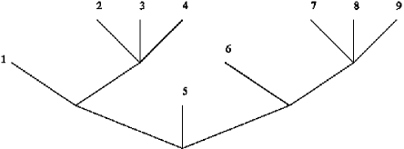
Figure 5. A finite tree ${\mathbf{t}}$ with labeled leaves.

Then consider all the subtrees that are attached to the branch between the root and the left-most leaf. All the left-most leaves of these subtrees are mapped on the children of the root of ${\mathbf{t}}_{\{0\}}$, they form the population at generation 1 of the tree ${\mathbf{t}}_{\{0\}}$. In Figure 6, the considered sub-trees are surrounded by dashed lines, and the leaves at generation 1 are labeled $\{2,5,6\}$. Remark that the sub-tree that contains the leaf 5 is reduced to a single node (this particular leaf).

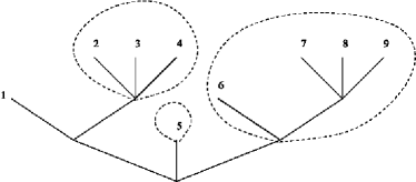
Figure 6. The sub-trees attached to the branch between the root and the leaf labeled 1.

Then perform the same procedure inductively at each of these sub-trees to construct the tree ${\mathbf{t}}_{\{0\}}$. In Figure 7, we give the tree ${\mathbf{t}}_{\{0\}}$ associated with the tree ${\mathbf{t}}$.

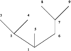
Figure 7. The tree ${\mathbf{t}}_{\{0\}}$ associated with the tree ${\mathbf{t}}$.

Using the branching property, we get that all the sub-trees that are attached to the left-most branch of a GW tree $\tau$ are independent and distributed as $\tau$. Therefore, the tree $\tau_{\{0\}}$ is still a GW tree.

Next, we compute the offspring distribution, $p_{\{0\}}$, of $\tau_{\{0\}}$. We denote by $N$ the generation of the left-most leaf. It is easy to see that this random variable is distributed according to a geometric distribution with parameter $p(0)$ i.e., for every $n\geq 1$,

$${\mathbb{P}}(N=n)=\bigl{(}1-p(0)\bigr{)}^{n-1}p(0).$$

Let $\zeta$ be a random variable with distribution $p$ and mean $m$. We denote by $(X_{1},\ldots,X_{N-1})$ the respective numbers of offsprings of the nodes on the left-most branch (including the root, excluding the leaf). Then, using again the branching property, these variables are independent, independent of $N$, and distributed as $\zeta$ conditionally on $\{\zeta>0\}$ i.e., for every $n\geq 1$,

$${\mathbb{P}}(X_{k}=n)=\frac{p(n)}{1-p(0)}\cdot$$

In particular, we have ${\mathbb{E}}[X_{k}]={m}/(1-p(0))$. Then, the number of children of the root in the tree $\tau_{\{0\}}$ is the number of the sub-trees attached to the left-most branch that is:

$$\zeta^{\prime}=\sum_{k=1}^{N-1}(X_{k}-1).$$

In particular, its mean is:

$${\mathbb{E}}\left[\zeta^{\prime}\right]={\mathbb{E}}[N-1]{\mathbb{E}}[X_{1}-1]=\left(\frac{1}{p(0)}-1\right)\left(\frac{m}{1-p(0)}-1\right)\\ =\frac{1}{p(0)}\Bigl{(}m-\bigl{(}1-p(0)\bigr{)}\Bigr{)}.$$

In particular, if the GW tree $\tau$ is critical ($m=1$), then ${\mathbb{E}}\left[\zeta^{\prime}\right]=1$, and thus the GW tree $\tau_{\{0\}}$ is also critical.

3.3.7. Conditioning on the number nodes with given out-degree, critical case

The result of Section 3.3.6 can be generalized as follows. Let ${\mathcal{A}}$ be a subset of ${\mathbb{N}}$ and for a tree ${\mathbf{t}}$, we define the subset of nodes with out-degree in ${\mathcal{A}}$:

$${\mathcal{L}}_{\mathcal{A}}({\mathbf{t}})=\{u\in{\mathbf{t}},\ k_{u}({\mathbf{t}})\in{\mathcal{A}}\}$$

and $L_{\mathcal{A}}({\mathbf{t}})={\rm Card}\;\bigl{(}{\mathcal{L}}_{\mathcal{A}}({\mathbf{t}})\bigr{)}$ its cardinal.

• If ${\mathcal{A}}={\mathbb{N}}$, $L_{\mathcal{A}}({\mathbf{t}})$ is the total number of nodes of ${\mathbf{t}}$,

• If ${\mathcal{A}}=\{0\}$, $L_{\mathcal{A}}({\mathbf{t}})$ is the total number of leaves of ${\mathbf{t}}$.

The functional $L_{\mathcal{A}}$ satisfies property (Additivity) with $D({\mathbf{t}},x)=L_{\mathcal{A}}({\mathbf{t}})-{\bf 1}_{\{0\in{\mathcal{A}}\}}\geq 0$, that is:

$$L_{\mathcal{A}}({\mathbf{t}}\circledast_{x}{\mathbf{t}}^{\prime})=L_{\mathcal{A}}({\mathbf{t}}^{\prime})+L_{\mathcal{A}}({\mathbf{t}})-{\bf 1}_{\{0\in{\mathcal{A}}\}}.$$

Moreover, there also exists a one-to-one correspondence, generalizing Minami’s correspondence, between the set ${\mathcal{L}}_{\mathcal{A}}({\mathbf{t}})$ conditionally on being positive and a tree ${\mathbf{t}}_{\mathcal{A}}$, see Rizzolo [39]. Moreover, if the initial tree is a critical GW tree $\tau$, the associated tree $\tau_{\mathcal{A}}$ is still a critical GW tree. In particular, we get the following lemma.

We define:

$$p({\mathcal{A}})=\sum_{n\in{\mathcal{A}}}p(n).$$

Lemma 3.26 ([39]).

Let $\tau$ be a critical GW tree with offspring distribution $p$ satisfying (13) and $p({\mathcal{A}})>0$. Then, conditionally on $\{L_{\mathcal{A}}(\tau)>0\}$, $L_{\mathcal{A}}(\tau)$ is distributed as $|\tau_{\mathcal{A}}|$, where $\tau_{\mathcal{A}}$ is a critical GW tree with offspring distribution $p_{{\mathcal{A}}}$ satisfying (13).

We then deduce the following corollary as a direct consequence of Lemma 3.19 and (iii) of Theorem 3.7.

Corollary 3.27.

Let $\tau$ be a critical GW tree with offspring distribution $p$ satisfying (13) and let $\tau^{*}$ be Kesten’s tree associated with $p$. Let $d_{\mathcal{A}}$ be the period of the offspring distribution $p_{\mathcal{A}}$ defined in Lemma 3.26. Let $\tau_{n}$ be a random tree distributed according to $\tau$ conditionally on $\left\{L_{\mathcal{A}}(\tau)\in[n,n+d_{\mathcal{A}})\right\}$ (resp. $\{L_{\mathcal{A}}(\tau)\geq n\}$). Then, we have:

$$\tau_{n}\;\xrightarrow[n\rightarrow\infty]{\textbf{(d)}}\tau^{*}.$$

3.3.8. Other results

The proof of Theorem 3.7 can be slighly modified to study a tree with randomly marked nodes: conditionally given the tree, we mark its nodes randomly, independently of each others, with a probability that depends only on the out-degree of the node. Then we obtain that a critical GW tree conditioned on having $n$ marked nodes still converges in distribution toward Kesten’s tree, see [1]. This allows to study a Galton-Watson tree conditioned on the number of protected nodes where a protected node is a node that is neither a leaf nor the parent of a leaf.

The same kind of ideas can also be used to study conditioned multi-type GW trees, see [6] where the limit is now multi-type Kesten’s tree. See also [37, 41] for other results on this topic.

Finally, recall that $Z_{n}$ represents the population size at generation $n$. Again, the proof of Theorem 3.7 can be adapted to prove that a critical GW tree with geometric offspring distribution conditioned on $\{Z_{n}=n^{\alpha}\}$ for $\alpha\in[1,2)$ converges in distribution toward Kesten’s tree, see[4]. But, with the same assumptions (critical geometric offspring distribution), the case $\alpha=2$ is more involved as the limiting tree does not satisfy the usual branching property: the numbers of offspring inside a generation are not independent, see [2]. See also [5] for local limits of super-critical (and some sub-critical) Galton-Watson trees when conditioning on $\{Z_{n}=a_{n}\}$ for different sequences $(a_{n},n\in{\mathbb{N}}^{*})$ of integers.

3.4. Conditioning on the number nodes with given out-degree, sub-critical case

Theorems 3.10 deals with sub-critical offspring distributions but for the conditioning on the height. We complete the picture of Theorem 3.7 by conditioning on $\{L_{\mathcal{A}}(\tau)=n\}$ in the sub-critical case.

3.4.1. An equivalent probability

Let $p$ be an offspring distribution and ${\mathcal{A}}\subset{\mathbb{N}}$. Recall $p({\mathcal{A}})=\sum_{n\in{\mathcal{A}}}p(n)$. We assume that $p({\mathcal{A}})>0$ and we define

$$I_{\mathcal{A}}=\Big{\{}\theta>0,\ \sum_{k\in{\mathcal{A}}}\theta^{k-1}p(k)<+\infty\quad\text{and}\quad\sum_{k\not\in{\mathcal{A}}}\theta^{k-1}p(k)\leq 1\Big{\}}.$$

For $\theta\in I_{\mathcal{A}}$, we set for every $k\in{\mathbb{N}}$,

$$p_{\theta}^{\mathcal{A}}(k)=\begin{cases}\theta^{k-1}p(k)&\mbox{if }k\not\in{\mathcal{A}},\\ c_{\mathcal{A}}(\theta)\theta^{k-1}p(k)&\mbox{if }k\in{\mathcal{A}},\end{cases}$$

where $c_{\mathcal{A}}(\theta)$ is a constant that makes $p_{\theta}^{\mathcal{A}}$ a probability measure on ${\mathbb{N}}$ namely

$$c_{\mathcal{A}}(\theta)=\frac{1-\sum_{k\not\in{\mathcal{A}}}\theta^{k-1}p(k)}{\sum_{k\in{\mathcal{A}}}\theta^{k-1}p(k)}\cdot$$

Remark that $I_{\mathcal{A}}$ is exactly the set of $\theta$ for which $p_{\theta}^{\mathcal{A}}$ is indeed a probability measure: if $\theta\not\in I_{\mathcal{A}}$, either the sums diverge and the constant $c_{\mathcal{A}}(\theta)$ is not well-defined, or it is negative. Remark also that $I_{\mathcal{A}}$ is an interval that contains 1, as $p_{1}^{\mathcal{A}}=p$.

The following proposition gives the connection between $p$ and $p^{\mathcal{A}}_{\theta}$.

Proposition 3.28.

Let $\tau$ be a GW tree with offspring distribution $p$. Let ${\mathcal{A}}\subset{\mathbb{N}}$ such that $p({\mathcal{A}})>0$ and let $\theta\in I_{\mathcal{A}}$. Let $\tau_{[\theta]}$ be a GW tree with offspring distribution $p_{\theta}^{\mathcal{A}}$. Then, the conditional laws of $\tau$ given $\{L_{\mathcal{A}}(\tau)=n\}$ and of $\tau_{[\theta]}$ given $\{L_{\mathcal{A}}(\tau_{[\theta]})=n\}$ are the same.

Notice that we don’t assume that $p$ is critical, sub-critical or super-critical in Proposition 3.28.

Remark 3.29.

Proposition 3.28 generalizes the results already obtained for the total progeny, ${\mathcal{A}}={\mathbb{N}}$, of [29] and for the number of leaves, ${\mathcal{A}}=\{0\}$, of [7].

Proof.

Let ${\mathbf{t}}\in{\mathbb{T}}_{0}$. Using (12) and the definition of $p_{\theta}^{\mathcal{A}}$, we have:

$${\mathbb{P}}(\tau_{[\theta]}={\mathbf{t}}) =\prod_{v\in{\mathbf{t}}}p_{\theta}^{\mathcal{A}}\bigl{(}k_{v}({\mathbf{t}})\bigr{)}$$

$$=\left(\prod_{k_{v}({\mathbf{t}})\in{\mathcal{A}}}c_{\mathcal{A}}(\theta)\theta^{k_{v}({\mathbf{t}})-1}p\bigl{(}k_{v}({\mathbf{t}})\bigr{)}\right)\,\left(\prod_{k_{v}({\mathbf{t}})\not\in{\mathcal{A}}}\theta^{k_{v}({\mathbf{t}})-1}p\bigl{(}k_{v}({\mathbf{t}})\bigr{)}\right)$$

$$=c_{\mathcal{A}}(\theta)^{L_{\mathcal{A}}({\mathbf{t}})}\theta^{\sum_{v\in{\mathbf{t}}}k_{v}({\mathbf{t}})-|{\mathbf{t}}|}\,\prod_{v\in{\mathbf{t}}}p\bigl{(}k_{v}({\mathbf{t}})\bigr{)}.$$

Since $\sum_{v\in{\mathbf{t}}}k_{v}({\mathbf{t}})=|{\mathbf{t}}|-1$, we deduce that:

(34) $${\mathbb{P}}(\tau_{[\theta]}={\mathbf{t}})=\frac{c_{\mathcal{A}}(\theta)^{L_{\mathcal{A}}({\mathbf{t}})}}{\theta}\,{\mathbb{P}}(\tau={\mathbf{t}}).$$

By summing (34) on $\{{\mathbf{t}}\in{\mathbb{T}}_{0},\,L_{\mathcal{A}}({\mathbf{t}})=n\}$, we obtain:

$${\mathbb{P}}\bigl{(}L_{\mathcal{A}}(\tau_{[\theta]})=n\bigr{)}=\frac{c_{\mathcal{A}}(\theta)^{n}}{\theta}{\mathbb{P}}\bigl{(}L_{\mathcal{A}}(\tau)=n\bigr{)}.$$

By dividing this equation term by term with (34), we get that for ${\mathbf{t}}\in{\mathbb{T}}_{0}$ such that $L_{\mathcal{A}}({\mathbf{t}})=n$, we have:

$${\mathbb{P}}(\tau={\mathbf{t}}|L_{\mathcal{A}}(\tau)=n)={\mathbb{P}}(\tau_{[\theta]}={\mathbf{t}}|L_{\mathcal{A}}(\tau_{[\theta]})=n).$$

This ends the proof as $\tau$ (resp. $\tau_{[\theta]}$) is a.s. finite on $\{L_{\mathcal{A}}(\tau)=n\}$ (resp. $\{L_{\mathcal{A}}(\tau_{[\theta]})=n\}$). ∎

3.4.2. The generic sub-critical case

Let $p$ be a sub-critical offspring distribution and let ${\mathcal{A}}\subset{\mathbb{N}}$ such that $p({\mathcal{A}})>0$. For $\theta\in I_{\mathcal{A}}$, we denote by $m^{\mathcal{A}}(\theta)$ the mean value of the probability $p_{\theta}^{\mathcal{A}}$.

Lemma 3.30 ([3], Lemma 5.2).

Let $p$ be a sub-critical offspring distribution satisfying (13) and ${\mathcal{A}}\subset{\mathbb{N}}$ such that $p({\mathcal{A}})>0$. There exists at most one $\theta\in I_{\mathcal{A}}$ such that $m^{\mathcal{A}}(\theta)=1$.

When it exists, we denote by $\theta_{\mathcal{A}}^{c}$ the unique solution of $m^{\mathcal{A}}(\theta)=1$ in $I_{\mathcal{A}}$ and we shall consider the critical offspring distribution:

(35) $$p^{(*)}=p_{\theta_{\mathcal{A}}^{c}}^{\mathcal{A}}.$$

Definition 3.31.

The offspring distribution $p$ is said to be generic for the set ${\mathcal{A}}$ if $\theta_{\mathcal{A}}^{c}$ exists.

Using Proposition 3.28 and Corollary 3.27, we immediately deduce the following result in the sub-critical generic case.

Proposition 3.32.

Let $p$ be a sub-critical offspring distribution satisfying (13) and let ${\mathcal{A}}\subset{\mathbb{N}}$ such that $p({\mathcal{A}})>0$. Assume that $p$ is generic for ${\mathcal{A}}$. Let $\tau$ be a GW tree with offspring distribution $p$ and let $\tau^{*}_{\mathcal{A}}$ be Kesten’s tree associated with the offspring distribution $p^{(*)}$ given by (35). Let $d^{*}$ be the period of the offspring distribution of $p^{(*)}_{\mathcal{A}}$ defined in Lemma 3.26. Let $\tau_{n}$ be a random tree distributed according to $\tau$ conditionally on $\left\{L_{\mathcal{A}}(\tau)\in[n,n+d^{*})\right\}$ (resp. $\{L_{\mathcal{A}}(\tau)\geq n\}$). Then, we have:

$$\tau_{n}\;\xrightarrow[n\rightarrow\infty]{\textbf{(d)}}\tau^{*}_{\mathcal{A}}.$$

3.4.3. The non-generic sub-critical case

In order to state precisely the general result, we shall consider the set ${\mathbb{T}}_{\infty}$ of trees that may have infinite nodes and extend the definition of the local convergence on this set.

For $u=u_{1}u_{2}\ldots u_{n}\in{\mathcal{U}}$, we set $|u|_{\infty}=\max\{n,\max\{u_{i},1\leq i\leq n\}\}$ and we define the associated restriction operator:

$$\forall n\in{\mathbb{N}},\ \forall{\mathbf{t}}\in{\mathbb{T}}_{\infty},\ r_{n}^{\infty}({\mathbf{t}})=\{u\in{\mathbf{t}},\ |u|_{\infty}\leq n\}.$$

For all tree ${\mathbf{t}}\in{\mathbb{T}}_{\infty}$, the restricted tree $r_{n}^{\infty}({\mathbf{t}})$ has height at most $n$ and all the nodes have at most $n$ offsprings (hence the tree $r_{n}^{\infty}({\mathbf{t}})$ is finite). We define also the associated distance, for all ${\mathbf{t}},{\mathbf{t}}^{\prime}\in{\mathbb{T}}_{\infty}$,

$$d_{\infty}({\mathbf{t}},{\mathbf{t}}^{\prime})=2^{-\sup\{n\in{\mathbb{N}},\ r_{n}^{\infty}({\mathbf{t}})=r_{n}^{\infty}({\mathbf{t}}^{\prime})\}}.$$

Remark that, for trees in ${\mathbb{T}}$, the topologies induced by the distance $\delta$ and the distance $d_{\infty}$ coincide. We will from now-on work on the space ${\mathbb{T}}_{\infty}$ endowed with the distance $d_{\infty}$. Notice that $({\mathbb{T}}_{\infty},d_{\infty})$ is compact.

If $p=(p(n),n\in{\mathbb{N}})$ is a sub-critical offspring distribution with mean $m<1$, we define $\tilde{p}=(\tilde{p}(n),n\in{\mathbb{N}})$ a probability distribution on ${\mathbb{N}}\cup\{+\infty\}$ by:

$$\tilde{p}(n)=np(n)\quad\text{for $n\in{\mathbb{N}}$ and}\quad\tilde{p}(+\infty)=1-m.$$

We define a new random tree on ${\mathbb{T}}_{\infty}$ that we denote by $\tilde{\tau}(p)$ in a way very similar to the definition of Kesten’s tree.

Definition 3.33.

Let $p$ be a sub-critical offspring distribution satisfying (13). The condensation tree $\tilde{\tau}$ associated with $p$ is a multi-type GW tree taking values in ${\mathbb{T}}_{\infty}$ and distributed as follows:

• Individuals are normal or special.

• The root of $\tilde{\tau}(p)$ special.

• A normal individual produces only normal individuals according to $p$.

• A special individual produces individuals according to the distribution $\tilde{p}$.

  • If it has a finite number of offsprings, then one of them chosen uniformly at random, is special, the others (if any) are normal.

  • If it has an infinite number of offsprings, then all of them are normal.

As we suppose that $p$ is sub-critical (i.e. $m<1$), then the condensation tree $\tilde{\tau}$ associated with $p$ has a.s. only one infinite node, and its random height is distributed as $G-1$, where $G$ has the geometric distribution with parameter $1-m$.

The next lemma completes Lemma 3.30. Recall definitions from Section 3.4.1. Set $\theta^{*}_{\mathcal{A}}=\sup I_{\mathcal{A}}$.

Lemma 3.34 ([3], Lemma 5.2).

Let $p$ be a sub-critical offspring distribution satisfying (13) and ${\mathcal{A}}\subset{\mathbb{N}}$ such that $p({\mathcal{A}})>0$. If for all $\theta\in I_{\mathcal{A}}$, $m^{\mathcal{A}}(\theta)<1$, that is $p$ is not generic for ${\mathcal{A}}$, then $\theta^{*}_{\mathcal{A}}$ belongs to $I_{\mathcal{A}}$.

When $p$ is not generic for ${\mathcal{A}}$, we shall consider the sub-critical offspring distribution:

$$\tilde{p}^{(*)}=p_{\theta_{\mathcal{A}}^{*}}^{\mathcal{A}}.$$

By using similar arguments (consequently more involved nevertheless) as for the critical case, we can prove the following result.

Proposition 3.35 ([3], Theorem 1.3).

Let $p$ be a sub-critical offspring distribution satisfying (13) and let ${\mathcal{A}}\subset{\mathbb{N}}$ such that $p({\mathcal{A}})>0$. Assume that $p$ is not generic for ${\mathcal{A}}$. Let $\tau$ be a GW tree with offspring distribution $p$ and let $\tilde{\tau}^{*}_{\mathcal{A}}$ be a condensation tree associated with the sub-critical offspring distribution $\tilde{p}^{(*)}$. Let $\tilde{d}^{*}$ be the period of the offspring distribution of $\tilde{p}^{(*)}_{\mathcal{A}}$ defined in Lemma 3.26. Let $\tau_{n}$ be a random tree distributed according to $\tau$ conditionally on $\left\{L_{\mathcal{A}}(\tau)\in[n,n+\tilde{d}^{*})\right\}$ (resp. $\{L_{\mathcal{A}}(\tau)\geq n\}$). Then, we have:

$$\tau_{n}\;\xrightarrow[n\rightarrow\infty]{\textbf{(d)}}\tilde{\tau}^{*}_{\mathcal{A}}.$$

Remark 3.36.

In [25], the conditioning on $\{M(\tau)=n\}$ where $M$ is the maximal out-degree is also studied in the sub-critical case. It is proven that, if the support of the offspring distribution $p$ is unbounded (for the conditioning to be valid), the conditioned sub-critical GW tree always converges in distribution to the condensation tree associated with $p$.

3.4.4. Generic and non-generic distributions

Let $p$ be a sub-critical offspring distribution satisfying (13). We shall give a criterion to say easily for which sets ${\mathcal{A}}$ the offspring distribution $p$ is generic. As we have $m<1$, we want to find a $\theta$ (which will be greater than 1) such that $m^{\mathcal{A}}(\theta)=1$. This problem is closely related to the radius $\rho\geq 1$ of convergence of the generating function of $p$, denoted by $g$.

We have the following result.

Lemma 3.37 ([3], Lemma 5.4).

Let $p$ be a sub-critical offspring distribution satisfying (13).

• If $\rho=+\infty$ or if ($\rho<+\infty$ and $g^{\prime}(\rho)\geq 1$), then $p$ is generic for any ${\mathcal{A}}\subset{\mathbb{N}}$ such that $p({\mathcal{A}})>0$.

• If $\rho=1$ (i.e. the probability $p$ admits no exponential moment), then $p$ is non-generic for every ${\mathcal{A}}\subset{\mathbb{N}}$ such that $p({\mathcal{A}})>0$.

• If $1<\rho<+\infty$ and $g^{\prime}(\rho)<1$, then $p$ is non-generic for ${\mathcal{A}}\subset{\mathbb{N}}$, with $p({\mathcal{A}})>0$, if and only if:

  $${\mathbb{E}}[Y|Y\in{\mathcal{A}}]<\frac{\rho-\rho g^{\prime}(\rho)}{\rho-g(\rho)},$$

  where $Y$ is distributed according to $p_{\rho}^{\mathbb{N}}$, that is

  $${\mathbb{E}}[f(Y)]={\mathbb{E}}[f(\zeta)\rho^{\zeta}]/g(\rho).$$

  In particular, $p$ is non-generic for ${\mathcal{A}}=\{0\}$ but generic of ${\mathcal{A}}=\{k\}$ for any $k$ large enough such that $p(k)>0$.

Remark 3.38.

In case (iii) of Lemma 3.37, we gave in Remark 5.5 of [3]:

• a sub-critical offspring distribution which is generic for ${\mathbb{N}}$ but non-generic for $\{0\}$;

• a sub-critical offspring distribution which is non-generic for ${\mathbb{N}}$ but generic for $\{k\}$ for $k$ large enough.

This shows that the genericity of sets is not monotone with respect to the inclusion.

References

- [1] R. ABRAHAM, A. BOUAZIZ, and J.-F. DELMAS. Local limits of Galton-Watson trees conditioned on the number of protected nodes. J. of Appl. Probab., 54:55–65, 2017.
- [2] R. ABRAHAM, A. BOUAZIZ, and J.-F. DELMAS. Very fat geometric Galton-Watson trees. arXiv:1709.09403, 2017.
- [3] R. ABRAHAM and J.-F. DELMAS. Local limits of conditioned Galton-Watson trees: the condensation case. Elec. J. of Probab., 19:Article 56, 1–29, 2014.
- [4] R. ABRAHAM and J.-F. DELMAS. Local limits of conditioned Galton-Watson trees: the infinite spine case. Elec. J. of Probab., 19:Article 2, 1–19, 2014.
- [5] R. ABRAHAM and J.-F. DELMAS. Asymptotic properties of expansive Galton-Watson trees. arXiv:1712.04650, 2017.
- [6] R. ABRAHAM, J.-F. DELMAS, and H. GUO. Critical multi-type galton-watson trees conditioned to be large. J. of Th. Probab., 31:757–788, 2018.
- [7] R. ABRAHAM, J.-F. DELMAS, and H. HE. Pruning Galton-Watson trees and tree-valued Markov processes. Ann. de l’Inst. Henri Poincaré, 48:688–705, 2012.
- [8] D. ALDOUS. The continuum random tree III. Ann. of Probab., 21:248–289, 1993.
- [9] D. ALDOUS and J. PITMAN. Tree-valued Markov chains derived from Galton-Watson processes. Ann. de l’Inst. Henri Poincaré, 34:637–686, 1998.
- [10] K. ATHREYA and P. NEY. Branching processes. Springer-Verlag, New York-Heidelberg, 1972. Die Grundlehren der mathematischen Wissenschaften, Band 196.
- [11] I. BIENAYME. De la loi de multiplication et de la durée des familles. Soc. Philomath. Paris Extraits, Sér. 5:37–39, 1845.
- [12] P. BILLINGSLEY. Convergence of probability measures. Wiley Series in Probability and Statistics: Probability and Statistics. John Wiley & Sons Inc., New York, second edition, 1999. A Wiley-Interscience Publication.
- [13] N. CURIEN and I. KORTCHEMSKI. Random non-crossing plane configurations: a conditioned Galton-Watson tree approach. Random Struct. and Alg., 45:236–260, 2014.
- [14] M. DRMOTA. Random trees. SpringerWienNewYork, Vienna, 2009. An interplay between combinatorics and probability.
- [15] M. DRMOTA and H. PRODINGER. The register function for -ary trees. ACM Trans. Algorithms, 2(3):318–334, 2006.
- [16] T. DUQUESNE. A limit theorem for the contour process of conditioned Galton-Watson trees. Ann. of Probab., 31:996–1027, 2003.
- [17] T. DUQUESNE and J.-F. LE GALL. Random trees, Lévy processes and spatial branching processes. Number 281. Astérisque, 2002.
- [18] R. DURRETT. Probability: theory and examples. Duxbury Press, Belmont, CA, second edition, 1996.
- [19] M. DWASS. The total progeny in a branching process and a related random walk. J. Appl. Probability, 6, 1969.
- [20] S. N. EVANS. Probability and real trees, volume 1920 of Lecture Notes in Mathematics. Springer, Berlin, 2008. Lectures from the 35th Summer School on Probability Theory held in Saint-Flour, July 6–23, 2005.
- [21] F. GALTON and H. WATSON. On the probability of extinction of families. J. Anthropol. Inst., 4:138–144, 1874.
- [22] P. HACCOU, P. JAGERS, and V. A. VATUTIN. Branching processes: variation, growth, and extinction of populations, volume 5 of Cambridge Studies in Adaptive Dynamics. Cambridge University Press, Cambridge; IIASA, Laxenburg, 2007.
- [23] T. E. HARRIS. The theory of branching processes. Die Grundlehren der Mathematischen Wissenschaften, Bd. 119. Springer-Verlag, Berlin; Prentice-Hall, Inc., Englewood Cliffs, N.J., 1963.
- [24] X. HE. Local convergence of critical random trees and continuum condensation tree. arXiv:1503.00951, 2015.
- [25] X. HE. Conditioning Galton-Watson trees on large maximal out-degree. J. of Th. Probab., 30:842–851, 2017.
- [26] S. JANSON. Simply generated trees, conditioned Galton-Watson trees, random allocations and condensation. Probab. Surv., 9:103–252, 2012.
- [27] T. JONNSSON and S. STEFANSSON. Condensation in nongeneric trees. J. Stat. Phys., 142:277–313, 2011.
- [28] D. G. KENDALL. The genealogy of genealogy: branching processes before (and after) 1873. Bull. London Math. Soc., 7(3):225–253, 1975.
- [29] D. KENNEDY. The Galton-Watson process conditioned on the total progeny. J. Appl. Probability, 12(4):800–806, 1975.
- [30] H. KESTEN. Subdiffusive behavior of random walk on a random cluster. Ann. Inst. H. Poincaré Probab. Statist., 22(4):425–487, 1986.
- [31] H. KESTEN and B. P. STIGUM. A limit theorem for multidimensional Galton-Watson processes. Ann. Math. Statist., 37:1211–1223, 1966.
- [32] M. KIMMEL and D. E. AXELROD. Branching processes in biology, volume 19 of Interdisciplinary Applied Mathematics. Springer-Verlag, New York, 2002.
- [33] R. LYONS, R. PEMANTLE, and Y. PERES. Conceptual proofs of criteria for mean behavior of branching processes. Ann. Probab., 23(3):1125–1138, 1995.
- [34] N. MIMAMI. On the number of vertices with a given degree in a Galton-Watson tree. Adv. in Appl. Probab., 37(1):229–264, 2005.
- [35] J. NEVEU. Sur le théorème ergodique de Chung-Erdős. C. R. Acad. Sci. Paris, 257:2953–2955, 1963.
- [36] J. NEVEU. Arbres et processus de Galton-Watson. Ann. de l’Inst. Henri Poincaré, 22:199–207, 1986.
- [37] S. PENISSON. Beyond the q-process: various ways of conditioning multitype Galton-Watson processes. ALEA, Lat. Am. J. Probab. Math. Stat., 13:223–237, 2016.
- [38] J. PITMAN. Combinatorial stochastic processes, volume 1875 of Lecture Notes in Mathematics. Springer-Verlag, Berlin, 2006. Lectures from the 32nd Summer School on Probability Theory held in Saint-Flour, July 7–24, 2002, With a foreword by Jean Picard.
- [39] D. RIZZOLO. Scaling limits of Markov branching trees and Galton-Watson trees conditioned on the number of vertices with out-degree in a given set. Ann. de l’Inst. Henri Poincaré, to appear, 2015.
- [40] F. SPITZER. Principles of random walk. Springer-Verlag, New York, second edition, 1976. Graduate Texts in Mathematics, Vol. 34.
- [41] R. STEPHENSON. Local convergence of large critical multi-type Galton-Watson trees and applications to random maps. J. of Th. Probab., 31:159–205, 2018.