Complexity certifications of first order inexact Lagrangian methods for general convex programming

Abstract

In this chapter we derive computational complexity certifications of first order inexact dual methods for solving general smooth blackconstrained convex problems which can arise in real-time applications, such as model predictive control. When it is difficult to project on the primal blackconstraint set described by a collection of general convex functions, we use the Lagrangian relaxation to handle the complicated constraints and then, we apply dual (fast) gradient algorithms based on inexact dual gradient information for solving the corresponding dual problem. The iteration complexity analysis is based on two types of approximate primal solutions: the primal last iterate and an average of primal iterates. We provide sublinear computational complexity estimates on the primal suboptimality and blackconstraint (feasibility) violation of the generated approximate primal solutions. In the final part of the chapter, we present an open-source quadratic optimization solver, blackreferred to as DuQuad, for convex quadratic programs and for evaluation of its behavior. The solver contains the C-language implementations of the analyzed algorithms.

1 Introduction

Nowadays, many engineering applications can be posed as general smooth blackconstrained convex problems. Several important applications that can be modeled in this framework blackhave attracted great attention lately, such as model predictive control for dynamical linear systems and its dual (often referred to as moving horizon estimation) NecFer:14c ; NedNec:14 ; PatBem:12j ; RicJon:12 ; RawMay:09 , DC optimal power flow problem for blackpower systems ZimMur:11 , blackand network utility maximization problems WeiOzd:10 . blackNotably, the recent advances in hardware and numerical optimization made it possible to solve linear model predictive control problems of nontrivial sizes within microseconds even on hardware platforms with limited computational power and memory.

In this chapter, we are particularly interested in real-time linear model predictive control (MPC) problems. For MPC, the corresponding optimal control problem can be recast as a smooth blackconstrained convex optimization problem. There are numerous ways in which this problem can be solved. For example, an interior point method has been proposed in RaoWri:98 and an active set method was described in FerKir:14 . Also, explicit MPC blackhas been proposed in BemMor:02 , where the optimization problem is solved off-line for all possible states. In blackreal-time (or on-line) applications, these methods can sometimes fail due to their overly complex iterations in the case of interior point and active set methods, or due to the large dimensions of the problem in the case of explicit blackMPCs. Additionally, when embedded systems are employed, computational complexities need to be kept to a minimum. As a result, second order algorithms (e.g. interior point), blackwhich most often require matrix inversions, are usually left out. blackIn such applications, first order algorithms are more suitable NecFer:14c ; NecNed:14b ; NedNec:14 ; PatBem:12j ; RicJon:12 blackespecially for instances when computation power and memory is limited. For many optimization problems arising in engineering applications, such as real-time blackMPCs, the constraints are overly complex, making projections on these sets blackcomputationally prohibitive. This is most often the main impediment of applying first order methods on the primal optimization problem. To circumvent this, the dual approach is considered blackby forming the dual problem, whereby the complex constraints are moved into the objective function, thus rendering much simpler constraints for the dual variables, often being only the non-negative orthant. blackTherefore, we consider dual first order methods for solving the dual problem. The computational complexity certification of gradient-based methods for solving the (augmented) Lagrangian dual of a primal convex problem is studied e.g. in BecNed:14 ; DevGli:11 ; KosNed ; NecPat:14 ; NecNed:14b ; NecNed:14a ; NedNec:14 ; NedOzd:08 ; PatBem:12j . However, these papers either threat quadratic problems PatBem:12j or linearly constrained smooth convex problems with simple objective function BecNed:14 ; NecPat:14 , or the approximate primal solution is generated through averaging NecNed:14b ; NecNed:14a ; NedNec:14 ; NedOzd:08 . On the other hand, in practice usually the last primal iterate is employed. There are few attempts to derive the computational complexity of dual gradient based methods using as an approximate primal solution the last iterate of the algorithm for particular cases of convex problems NecNed:14a ; NecPat:14 ; BecNed:14 . Moreover, from our practical experience we have observed that usually these methods converge faster in the primal last iterate than in a primal average sequence. These issues motivate our work here.

Contribution. In this chapter, we analyze the computational complexity of dual first order methods for solving general smooth blackconstrained convex problems. Contrary to most of the results from the literature BecNed:14 ; NecPat:14 ; NecNed:14a ; NedOzd:08 ; PatBem:12j , our approach allows us to use inexact dual gradient information. Another important feature of our approach is that we blackalso provide complexity results for the primal latest iterate, while in much of the previous literature convergence rates in an average of primal iterates are given. This feature is of practical importance since usually the primal last iterate is employed in applications. More precisely, the main contributions in this chapter are:

$(i)$ We derive the computational complexity of the dual gradient method in terms of primal suboptimality and feasibility violation using inexact dual gradients and two types of approximate primal solutions: $\mathcal{O}\left(\frac{1}{\epsilon^{2}}\log\frac{1}{\epsilon}\right)$ in the primal last iterate and $\mathcal{O}\left(\frac{1}{\epsilon}\log\frac{1}{\epsilon}\right)$ in an average of primal iterates, where $\epsilon$ is some desired accuracy.

$(ii)$ We also derive the computational complexity of the dual fast gradient method in terms of primal suboptimality and feasibility violation using inexact dual gradients and two types of approximate primal solutions: $\mathcal{O}\left(\frac{1}{\epsilon}\log\frac{1}{\epsilon}\right)$ in the primal last iterate and $\mathcal{O}\left(\frac{1}{\sqrt{\epsilon}}\log\frac{1}{\epsilon}\right)$ in a primal average sequence.

$(iii)$ Finally, we present an open-source optimization solver, blacktermed DuQuad, consisting of the C-language implementations of the above inexact dual first order algorithms for solving convex quadratic problems, and blackwe study its numerical behavior.

blackContent. The chapter is organized as follows. In Section 2 we formulate our problem of interest and its dual, and blackwe analyze its smoothness property. In Section 3 we introduce a general inexact dual first order method, covering the inexact dual gradient and fast gradient algorithms, and blackwe derive computational complexity certificates for these schemes. Finally, in Section 4 we describe briefly the DuQuad toolbox blackthat implements the above inexact algorithms for solving convex quadratic programs in C-language, while in Section 5 we provide detailed numerical experiments.

blackNotation. We consider the space $\mathbb{R}^{n}$ composed blackof column vectors. For $\mathbf{x},\mathbf{y}\in\mathbb{R}^{n}$, blackwe denote the scalar product by $\langle\mathbf{x},\mathbf{y}\rangle=\mathbf{x}^{T}\mathbf{y}$ and the Euclidean norm by $\|\mathbf{x}\|=\sqrt{\mathbf{x}^{T}\mathbf{x}}$. We denote the nonnegative orthant by $\mathbb{R}^{n}_{+}$ and blackwe use $[\mathbf{u}]_{+}$ for the projection of $\mathbf{u}$ onto $\mathbb{R}^{n}_{+}$. The minimal eigenvalue of a symmetric matrix $\mathbf{Q}\in\mathbb{R}^{n\times n}$ is denoted by $\lambda_{\min}(\mathbf{Q})$ and $\|\mathbf{Q}\|_{F}$ denotes its Frobenius norm.

2 Problem formulation

In this blacksection, we consider the following general blackconstrained convex optimization problem:

$$f^{*}=\min_{\mathbf{u}\in U} \;\;f(\mathbf{u})\qquad\text{s.t.:}\;\;\mathbf{g}(\mathbf{u})\leq{\mathbf{0}},$$ (1)

where $U\subseteq\mathbb{R}^{n}$ is a closed simple convex set (e.g. a box set), ${\mathbf{0}}\in\mathbb{R}^{p}$ is a vector of zeros, and blackthe constraint mapping $\mathbf{g}(\cdot)$ is given by $\mathbf{g}(\cdot)=\textcolor{black}{[g_{1}(\cdot),\ldots,}g_{p}(\cdot)]^{T}$. (The vector inequality $\mathbf{g}(\mathbf{u})\leq{\mathbf{0}}$ is to be understood coordinate-wise.) The objective function $f(\cdot)$ and the constraint functions $g_{1}(\cdot),\ldots,g_{p}(\cdot)$ are convex and differentiable over their domains. Many engineering applications can be posed as the general convex problem (1). blackFor example for linear model predictive control problem in condensed form NecFer:14c ; NedNec:14 ; PatBem:12j ; RicJon:12 ; RawMay:09 : $f$ is convex (quadratic) function, $U$ is box set describing the input constraints and $\mathbf{g}$ is blackgiven by convex functions describing the state constraints; blackfor network utility maximization problem BecNed:14 : $f$ is $\log$ function, $U=\mathbb{R}^{n}_{+}$ and $\mathbf{g}$ is linear function describing the link capacities; blackfor DC optimal power flow problem ZimMur:11 : $f$ is convex function, $U$ is box set and $\mathbf{g}$ describes the DC nodal power balance constraints.

We are interested in deriving computational complexity estimates of dual first order methods for solving the optimization problem (1). We make the following assumptions on the objective function and the feasible set of the problem (1).

Assumption 1

black Let $U\subseteq\text{dom}\ f\cap\left\{\cap_{i=1}^{p}\text{dom}\ g_{i}\right\}$, and assume that:

black (a) The Slater condition holds for the feasible set of problem (1), i.e., there exists $\bar{\mathbf{u}}\in\text{relint}(U)$ such that $\mathbf{g}(\bar{\mathbf{u}})<{\mathbf{0}}$.

(b) The function $f$ is strongly convex with constant $\sigma_{f}>0$ and has Lipschitz continuous blackgradients with constant $L_{f}$, i.e.:

$$\frac{\sigma_{f}}{2}\lVert\mathbf{u}-\mathbf{v}\rVert^{2}\leq f(\mathbf{u})-\left(f(\mathbf{v})+\langle\nabla f(\mathbf{v}),\mathbf{u}-\mathbf{v}\rangle\right)\leq\frac{L_{f}}{2}\lVert\mathbf{u}-\mathbf{v}\rVert^{2}\quad\forall\mathbf{u},\mathbf{v}\in U.$$

(c) The function $\mathbf{g}$ has bounded Jacobians on the set $U$, i.e., there exists $c_{g}>0$ such that $\|\nabla\mathbf{g}(\mathbf{u})\|_{F}\leq c_{g}$   for all $\mathbf{u}\in U$.

Moreover, we introduce the following definition:

Definition 1

Given $\epsilon>0$, a primal point $\mathbf{u}_{\epsilon}\in U$ is called $\epsilon$-optimal if it satisfies:

$$|f(\mathbf{u}_{\epsilon})-f^{*}|\leq\epsilon\quad\text{and}\quad\left\|\left[\mathbf{g}(\mathbf{u}_{\epsilon})\right]_{+}\right\|\leq\epsilon.$$

Since $U$ is assumed to be a simple set, i.e. the projection on this set is easy (e.g. a box set), we denote the associated dual problem of (1) as:

$$\max_{\mathbf{x}\geq 0}\;d(\mathbf{x})\quad\left(=\min_{\mathbf{u}\in U}\mathcal{L}(\mathbf{u},\mathbf{x})\right),$$ (2)

where the Lagrangian function is given by:

$$\mathcal{L}(\mathbf{u},\mathbf{x})=f(\mathbf{u})+\langle\mathbf{x},\mathbf{g}(\mathbf{u})\rangle.$$

We denote the dual optimal set with black$X^{*}=\arg\max\limits_{\mathbf{x}\geq{\mathbf{0}}}d(\mathbf{x})$. Note that Assumption 1$(a)$ guarantees that strong duality holds for (1). Moreover, since $f$ is strongly convex function (see Assumption 1$(b)$), the inner subproblem $\min\limits_{\mathbf{u}\in U}\mathcal{L}(\mathbf{u},\mathbf{x})$ has the objective function $\mathcal{L}(\cdot,\mathbf{x})$ strongly convex for any fixed $\mathbf{x}\in\mathbb{R}^{p}_{+}$. It follows that the optimal solution $\mathbf{u}^{*}$ of the original problem (1) and $\mathbf{u}(\mathbf{x})=\arg\min_{\mathbf{u}\in U}\mathcal{L}(\mathbf{u},\mathbf{x})$ are unique and, thus, from Danskin’s theorem Nes:05 we get that the dual function $d$ is differentiable on $\mathbb{R}^{n}_{+}$ and its gradient is given by:

$$\nabla d(\mathbf{x})=\mathbf{g}(\mathbf{u}(\mathbf{x}))\qquad\hbox{for all $\mathbf{x}\in\mathbb{R}^{n}_{+}$}.$$

From Assumption 1$(c)$ it follows immediately, using the mean value theorem, that the function $\mathbf{g}$ is Lipschitz continuous with constant $c_{g}$, i.e.,

$$\|\mathbf{g}(\mathbf{u})-\mathbf{g}(\mathbf{v})\|\leq c_{g}\|\mathbf{u}-\mathbf{v}\|\qquad\forall\mathbf{u},\mathbf{v}\in U.$$ (3)

blackIn the forthcoming lemma, Assumption 1 $(b)$ and $(c)$ allow us to show that the dual function $d$ has Lipschitz gradient. Our result is a generalization of a result in Nes:05 given there for the case of blacka linear mapping $\mathbf{g}(\cdot)$ (see also NecNed:14b for a different proof):

Lemma 1

Under Assumption 1, the dual function black$d(\cdot)$ corresponding to general convex problem (1) has Lipschitz continuous gradient with constant $L_{\text{d}}=c_{g}^{2}/\sigma_{f}$, i.e.,

$$\|\nabla d(\mathbf{x})-\nabla d(\bar{\mathbf{x}})\|\leq c_{g}^{2}/\sigma_{f}\|\mathbf{x}-\bar{\mathbf{x}}\|\qquad\forall\mathbf{x},\bar{\mathbf{x}}\in\mathbb{R}^{p}_{+}.$$ (4)

Proof

Let $\mathbf{x},\bar{\mathbf{x}}\in\mathbb{R}^{p}_{+}$. blackThen, by using the optimality conditions for $\mathbf{u}(\mathbf{x})$ and $\mathbf{u}(\bar{\mathbf{x}})$, we get:

$$\left\langle\nabla f(\mathbf{u}(\mathbf{x}))+\sum_{i=1}^{p}\mathbf{x}_{i}\nabla g_{i}(\mathbf{u}(\mathbf{x})),\mathbf{u}(\bar{\mathbf{x}})-\mathbf{u}(\mathbf{x})\right\rangle\geq 0,$$

$$\left\langle\nabla f(\mathbf{u}(\bar{\mathbf{x}}))+\sum_{i=1}^{p}\bar{\mathbf{x}}_{i}\nabla g_{i}(\mathbf{u}(\bar{\mathbf{x}})),\mathbf{u}(\mathbf{x})-\mathbf{u}(\bar{\mathbf{x}})\right\rangle\geq 0.$$

Adding blackthese two inequalities and using the strong convexity of $f$, we blackfurther obtain

$$\sigma_{f}\|\mathbf{u}(\mathbf{x})-\mathbf{u}(\bar{\mathbf{x}})\|^{2}\leq\langle\nabla f(\mathbf{u}(\mathbf{x}))-\nabla f(\mathbf{u}(\bar{\mathbf{x}})),\mathbf{u}(\mathbf{x})-\mathbf{u}(\bar{\mathbf{x}})\rangle$$

$$\leq\left\langle\sum_{i}\mathbf{x}_{i}\nabla g_{i}(\mathbf{u}(\mathbf{x}))-\sum_{i}\bar{\mathbf{x}}_{i}\nabla g_{i}(\mathbf{u}(\bar{\mathbf{x}})),\mathbf{u}(\bar{\mathbf{x}})-\mathbf{u}(\mathbf{x})\right\rangle$$

$$=\left\langle\textcolor{black}{\sum_{i=1}^{p}}(\mathbf{x}_{i}-\bar{\mathbf{x}}_{i})\nabla g_{i}(\mathbf{u}(\mathbf{x}))\!-\!\textcolor{black}{\sum_{i=1}^{p}}\bar{\mathbf{x}}_{i}(\nabla g_{i}(\mathbf{u}(\bar{\mathbf{x}}))-\nabla g_{i}(\mathbf{u}(\mathbf{x}))),\mathbf{u}(\bar{\mathbf{x}})-\mathbf{u}(\mathbf{x})\right\rangle$$

$$\leq\left\langle\!\textcolor{black}{\sum_{i=1}^{p}}(\mathbf{x}_{i}\!-\!\bar{\mathbf{x}}_{i})\nabla g_{i}(\mathbf{u}(\mathbf{x})),\mathbf{u}(\bar{\mathbf{x}})\!-\!\mathbf{u}(\mathbf{x})\!\!\right\rangle,$$

blackwhere the last inequality follows from the convexity of the function $g_{i}$ and $\bar{\mathbf{x}}_{i}\geq 0$ for all $i$. By the Cauchy-Schwarz inequality, we have

$$\sigma_{f}\|\mathbf{u}(\mathbf{x})-\mathbf{u}(\bar{\mathbf{x}})\|^{2} \leq\textcolor{black}{\sum_{i=1}^{p}}|\mathbf{x}_{i}\!-\!\bar{\mathbf{x}}_{i}|\|\nabla g_{i}(\mathbf{u}(\mathbf{x}))\|\|\mathbf{u}(\mathbf{x})\!-\!\mathbf{u}(\bar{\mathbf{x}})\|$$

$$\leq\|\mathbf{x}-\bar{\mathbf{x}}\|\|\nabla\mathbf{g}(\mathbf{u}(\mathbf{x}))\|_{F}\|\mathbf{u}(\mathbf{x})-\mathbf{u}(\bar{\mathbf{x}})\|$$

$$\leq c_{g}\|\mathbf{x}-\bar{\mathbf{x}}\|\|\mathbf{u}(\mathbf{x})-\mathbf{u}(\bar{\mathbf{x}})\|,$$

blackwhere the second inequality follows by Hölder’s inequality and the last inequality follows by the bounded Jacobian assumption for $\mathbf{g}$ (see Assumption 1(c$)$). Thus, we obtain:

$$\|\mathbf{u}(\mathbf{x})-\mathbf{u}(\bar{\mathbf{x}})\|\leq\frac{c_{g}}{\sigma_{f}}\|\mathbf{x}-\bar{\mathbf{x}}\|.$$

Combining (3) with the blackpreceding relation, we obtain that the gradient of the dual function is Lipschitz continuous with constant black$L_{\text{d}}=\frac{c_{g}^{2}}{\sigma_{f}}$, i.e.,

$$\|\nabla d(\mathbf{x})-\nabla d(\bar{\mathbf{x}})\| =\|\mathbf{g}(\mathbf{u}(\mathbf{x}))-\mathbf{g}(\mathbf{u}(\bar{\mathbf{x}}))\|\leq c_{g}\|\mathbf{u}(\mathbf{x})-\mathbf{u}(\bar{\mathbf{x}})\|\leq\frac{c_{g}^{2}}{\sigma_{f}}\|\mathbf{x}-\bar{\mathbf{x}}\|,$$

for all $\mathbf{x},\bar{\mathbf{x}}\in\mathbb{R}^{p}_{+}$. ∎

Note that in the case blackof a linear mapping $\mathbf{g}$, i.e., $\mathbf{g}(\mathbf{u})=\mathbf{Gu}+\mathbf{g}$, blackwe have $c_{g}=\|\mathbf{G}\|_{F}\geq\|\mathbf{G}\|$. In conclusion, blackour estimate on the Lipschitz constant of the gradient of the dual function for general convex constraints $L_{\text{d}}=c_{g}^{2}/\sigma_{f}$ can coincide with the one derived in Nes:05 for the linear case $L_{\text{d}}=\|\mathbf{G}\|^{2}/\sigma_{f}$ blackif one takes the linear structure of $\mathbf{g}$ into account in the proof of Lemma 1 (specifically, where we used Hölder’s inequality). Based blackon relation (4) of Lemma 1, the following descent lemma holds with $L_{\text{d}}=c_{g}^{2}/\sigma_{f}$ (see for example Nes:05 ):

$$d(\mathbf{x})\geq d(\mathbf{y})+\langle\nabla d(\mathbf{y}),\mathbf{x}-\mathbf{y}\rangle-\frac{L_{\text{d}}}{2}\lVert\mathbf{x}-\mathbf{y}\rVert^{2}\quad\forall\mathbf{x},\mathbf{y}\in\mathbb{R}^{p}_{+}.$$ (5)

Using these preliminary results, blackin a unified manner, we analyze further the computational complexity of inexact dual first order methods.

3 Inexact dual first order methods

In this section we introduce and analyze inexact blackfirst order dual algorithms for solving the general smooth convex problem (1). Since the computation of the zero-th and blackthe first order information of the dual problem (2) requires the exact solution of the inner subproblem $\min\limits_{\mathbf{u}\in U}\mathcal{L}(\mathbf{u},\mathbf{x})$ for some fixed $\mathbf{x}\in\mathbb{R}^{p}_{+}$, which generally cannot be computed in practice. blackIn many practical cases, inexact dual information is available by solving the inner subproblem with a certain inner accuracy. blackWe denote with $\tilde{\mathbf{u}}(\mathbf{x})$ the primal point satisfying the $\delta$-optimality relations:

$$\tilde{\mathbf{u}}(\mathbf{x})\in U,\qquad 0\leq\mathcal{L}(\tilde{\mathbf{u}}(\mathbf{x}),\mathbf{x})-d(\mathbf{x})\leq\delta\qquad\forall\mathbf{x}\in\mathbb{R}^{p}_{+}.$$ (6)

In relation with (6), we introduce the following approximations for the dual function and its gradient:

$$\tilde{d}(\mathbf{x})=\mathcal{L}(\tilde{\mathbf{u}}(\mathbf{x}),\mathbf{x})\quad\text{and}\quad\tilde{\nabla}d(\mathbf{x})=\mathbf{g}(\tilde{\mathbf{u}}(\mathbf{x})).$$

Then, the following bounds for the dual function $d(\mathbf{x})$ can be obtained, in terms of a linear and a quadratic model, which use only approximate information of the dual function and of its gradient (see (NecNed:14b, , Lemma 2.5)):

$$0\leq\left(\tilde{d}(\mathbf{y})+\langle\tilde{\nabla}d(\mathbf{y}),\mathbf{x}-\mathbf{y}\rangle\right)-d(\mathbf{x})\leq L_{d}\lVert\mathbf{x}-\mathbf{y}\rVert^{2}+3\delta\quad\forall\mathbf{x},\mathbf{y}\in\mathbb{R}^{p}_{+}.$$ (7)

Note that if $\delta=0$, then we recover the exact descent lemma (5). Before we introduce our algorithmic scheme, blacklet us observe that blackone can efficiently solve approximately the inner subproblem if the constraint functions $g_{i}(\cdot)$ satisfy certain assumptions, blacksuch as either one of the following conditions:

• The operator $\mathbf{g}(\cdot)$ is simple, i.e., given $\mathbf{v}\in U$ and $\mathbf{x}\in\mathbb{R}^{p}_{+}$, the solution of the following optimization subproblem:

  $$\min\limits_{\mathbf{u}\in U}\;\left\{\frac{1}{2}\lVert\mathbf{u}-\mathbf{v}\rVert^{2}+\langle\mathbf{x},\mathbf{g}(\mathbf{u})\rangle\right\}$$

  can be obtained in linear time, i.e. $\mathcal{O}(n)$ operations. An example satisfying this assumption is the linear operator, i.e. $\mathbf{g}(\mathbf{u})=\mathbf{Gu}+\mathbf{g}$, where $\mathbf{G}\in\mathbb{R}^{p\times n},\mathbf{g}\in\mathbb{R}^{p}$.

• Each function $g_{i}(\cdot)$ has Lipschitz blackcontinuous gradients.

blackIn such cases, based on Assumption 1(b) (i.e. $f$ has Lipschitz continuous gradient), it follows that we can solve approximately the inner subproblem $\min\limits_{\mathbf{u}\in U}\mathcal{L}(\mathbf{u},\mathbf{x})$, for any fixed $\mathbf{x}\in\mathbb{R}^{p}_{+}$, with Nesterov’s optimal method for convex problems with smooth and strongly convex objective function Nes:13 . Without blackloss of generality, we assume that the functions $g_{i}(\cdot)$ are simple. blackWhen $\mathbf{g}(\cdot)$ satisfies the above condition (2), there are minor modifications in the constants related to the convergence rate. Given $\mathbf{x}\in\mathbb{R}^{p}_{+}$, the inner approximate optimal point $\tilde{\mathbf{u}}(\mathbf{x})$ satisfying $\mathcal{L}(\tilde{\mathbf{u}}(\mathbf{x}),\mathbf{x})-d(\mathbf{x})\leq\delta$ is obtained with Nesterov’s optimal method Nes:13 blackafter $N_{\delta}$ projections on the simple set $U$ and evaluations of $\nabla f$, where

$$N_{\delta}=\left\lfloor\sqrt{\frac{L_{f}}{\sigma_{f}}}\log\left(\frac{L_{f}R_{p}^{2}({\mathbf{x}})}{2\delta}\right)\right\rfloor$$ (8)

with $R_{p}({\mathbf{x}})=\lVert\mathbf{v}^{0}-\mathbf{u}(\mathbf{x})\rVert$, and $\mathbf{v}^{0}$ being the initial point of Nesterov’s optimal method. blackWhen the simple feasible set $U$ is compact with a diameter $R_{p}$ (such as for example in MPC applications), we can bound black$R_{p}(\mathbf{x})$ uniformly, i.e.,

$$R_{p}(\mathbf{x})\leq R_{p}\qquad\forall\mathbf{x}\in\mathbb{R}^{p}_{+}.$$

In the sequel, we always assume that such a bound exists, and we use warm-start when solving the inner subproblem. Now, we introduce a general algorithmic scheme, called Inexact Dual First Order Method (IDFOM), and analyze its convergence properties, computational complexity and blacknumerical performance.

Algorithm IDFOM

Given $\mathbf{y}^{0}\in\mathbb{R}^{p}_{+},\;\delta>0$,   for $k\geq 0$ compute:

1.   Find $\mathbf{u}^{k}\in U$ such that $\mathcal{L}(\mathbf{u}^{k},\mathbf{y}^{k})-d(\mathbf{y}^{k})\leq\delta$,

2.   Update ${\mathbf{x}}^{k}=\left[\mathbf{y}^{k}+\frac{1}{2L_{\text{d}}}\tilde{\nabla}d(\mathbf{y}^{k})\right]_{+}$,

3.   Update $\mathbf{y}^{k+1}=\left(1-\theta_{k}\right)\mathbf{x}^{k}+\theta_{k}\left[\mathbf{y}^{0}+\frac{1}{2L_{\text{d}}}\sum\limits_{j=0}^{k}\frac{j+1}{2}\tilde{\nabla}d(\mathbf{y}^{j})\right]_{+}$.

where $\mathbf{u}^{k}=\tilde{\mathbf{u}}(\mathbf{y}^{k})$, $\tilde{\nabla}d(\mathbf{y}^{k})=\mathbf{g}(\mathbf{u}^{k})$ and blackthe selection of the parameter $\theta_{k}$ is discussed next. More precisely, we distinguish two particular well-known schemes of the above framework:

• IDGM: by setting $\theta_{k}=0$ blackfor all $k\geq 0$, we recover the Inexact Dual Gradient Method since $\mathbf{y}^{k+1}=\mathbf{x}^{k}$. For this scheme, we define the dual average sequence $\hat{\mathbf{x}}^{k}=\frac{1}{k+1}\sum\limits_{j=0}^{k}\mathbf{x}^{j}$. We redefine the dual final point (the dual last iterate $\mathbf{x}^{k}$ when some stopping criterion is satisfied) as $\mathbf{x}^{k}=\left[\hat{\mathbf{x}}^{k}+\frac{1}{2L_{\text{d}}}\tilde{\nabla}d(\hat{\mathbf{x}}^{k})\right]_{+}$. Thus, all the results concerning $\mathbf{x}^{k}$ generated by the algorithm IDGM will refer to this definition.

• IDFGM: by setting $\theta_{k}=\frac{2}{k+3}$ blackfor all $k\geq 0$, we recover the Inexact Dual Fast Gradient Method. This variant has been analyzed in Nes:05 ; DevGli:11 ; NecNed:14b .

Note that both dual sequences are dual feasible, i.e., $\mathbf{x}^{k},\mathbf{y}^{k}\in\mathbb{R}^{p}_{+}$ blackfor all $k\geq 0$, and thus the inner subproblem $\min\limits_{\mathbf{u}\in U}\mathcal{L}(\mathbf{u},\mathbf{y}^{k})$ has the objective function strongly convex. Towards estimating the computational complexity of IDFOM, we present an unified outer convergence rate for both schemes IDGM and IDFGM of algorithm IDFOM in terms of dual suboptimality. The result has been proved in DevGli:11 ; NecNed:14b .

Theorem 3.1

DevGli:11 ; NecNed:14b Given $\delta>0$, let black$\{(\mathbf{x}^{k},\mathbf{y}^{k})\}_{k\geq 0}$ be the dual sequences generated by algorithm IDFOM. Under Assumption 1, the following relation holds:

$$f^{*}-d(\mathbf{x}^{k})\leq\frac{L_{\text{d}}R_{d}^{2}}{k^{p(\theta)}}+4k^{p(\theta)-1}\delta\textcolor{black}{\qquad\forall k\geq 1,}$$

where $p(\theta)=\begin{cases}1,&\text{if}\;\;\theta_{k}=0\\ 2,&\text{if}\;\;\theta_{k}=\frac{2}{k+3}\end{cases}$  and  $R_{d}=\min\limits_{\mathbf{x}^{*}\in X^{*}}\;\lVert\mathbf{y}^{0}-\mathbf{x}^{*}\rVert$.

Proof

Firstly, consider the case $\theta_{k}=0$ (which implies $p(\theta)=1$). Note that the approximate convexity and Lipschitz continuity relations (7) lead to:

$$d(\mathbf{x}^{k}) \geq\tilde{d}(\hat{\mathbf{x}}^{k})+\langle\tilde{\nabla}d(\hat{\mathbf{x}}^{k}),\mathbf{x}^{k}-\hat{\mathbf{x}}^{k}\rangle-L_{\text{d}}\lVert\mathbf{x}^{k}-\hat{\mathbf{x}}^{k}\rVert^{2}-3\delta$$

$$\geq\tilde{d}(\hat{\mathbf{x}}^{k})+L_{\text{d}}\lVert\mathbf{x}^{k}-\hat{\mathbf{x}}^{k}\rVert^{2}-3\delta$$ (9)

$$\overset{\eqref{in:inexact_inner_opt}}{\geq}d(\hat{\mathbf{x}}^{k})-3\delta,$$ (10)

where in the second inequality we have used the optimality conditions of $\mathbf{x}^{k}=[\hat{\mathbf{x}}^{k}+\frac{1}{2L_{\text{d}}}\tilde{\nabla}d(\hat{\mathbf{x}}^{k})]_{+}\in\mathbb{R}^{p}_{+}$. On the other hand, using (DevGli:11, , Theorem 2), blackthe following convergence rate for the dual average point $\hat{\mathbf{x}}^{k}$ can be derived:

$$f^{*}-d(\hat{\mathbf{x}}^{k})\leq\frac{L_{\text{d}}R_{d}^{2}}{2k}+\delta\textcolor{black}{\qquad\forall k\geq 1}.$$ (11)

Combining (3) and (11) we blackobtain the first case of the theorem. blackThe second case, concerning $\theta_{k}=\frac{2}{k+3}$, has been shown in DevGli:11 ; NecNed:14b . ∎

Our iteration complexity analysis for algorithm IDFOM is based on two types of approximate primal solutions: the primal last iterate sequence $(\mathbf{v}^{k})_{k\geq 0}$ defined by $\mathbf{v}^{k}=\tilde{\mathbf{u}}(\mathbf{x}^{k})$ or a primal average sequence $(\hat{\mathbf{u}}^{k})_{k\geq 0}$ of the form:

$$\hat{\mathbf{u}}^{k}=\begin{cases}\frac{1}{k+1}\sum\limits_{j=0}^{k}\mathbf{u}^{j},&\text{if}\;\;\textbf{IDGM}\\ \textcolor{black}{\frac{2}{(k+1)(k+2)}\sum\limits_{j=0}^{k}(j+1)\mathbf{u}^{j}},&\text{if}\;\;\textbf{IDFGM}.\end{cases}$$ (12)

Note that for algorithm IDGM we have $\mathbf{v}^{k}=\mathbf{u}^{k}$, while for algorithm IDFGM $\mathbf{v}^{k}\not=\mathbf{u}^{k}$. Without blackloss of generality, for the simplicity of our results, we assume:

$$\mathbf{y}^{0}=0,\qquad R_{d}\geq\max\left\{1,\frac{1}{c_{g}},\frac{\textcolor{black}{L_{f}}}{c_{g}}\right\},\qquad L_{\text{d}}\geq 1.$$ (13)

If any of these conditions do not hold, then all of the results from below are valid with minor variations in the constants.

3.1 Computational complexity of IDFOM in primal last iterate

In this section we derive the computational complexity for the two main algorithms blackwithin the framework of IDFOM, in terms of primal feasibility violation and primal suboptimality for the last primal iterate $\mathbf{v}^{k}=\tilde{\mathbf{u}}(\mathbf{x}^{k})$. To obtain these results, only in this section, we additionally make the following assumption:

Assumption 2

The primal set $U$ is compact, i.e. $\max\limits_{\mathbf{u},\mathbf{v}\in U}\lVert\mathbf{u}-\mathbf{v}\rVert=R_{p}<\infty$.

Assumption 2 implies that the objective function $f$ is Lipschitz continuous with constant $\bar{L}_{f}$, where $\bar{L}_{f}=\max\limits_{\mathbf{u}\in U}\;\lVert\nabla f(\mathbf{u})\rVert$. Now, we are ready to prove the main result of this section, blackgiven in the following theorem.

Theorem 3.2

Let $\epsilon>0$ be some desired accuracy and $\mathbf{v}^{k}=\tilde{\mathbf{u}}(\mathbf{x}^{k})$ be the primal last iterate generated by algorithm IDFOM. Under Assumptions 1 and 2, by setting:

$$\delta\leq\frac{L_{\text{d}}R_{d}^{2}}{2\alpha^{p(\theta)-1}}\left(\frac{\epsilon}{6L_{\text{d}}R_{d}^{2}}\right)^{4-2/p(\theta)},$$ (14)

where $\alpha=\max\left\{1,\left(\frac{\bar{L}_{f}}{c_{g}R_{d}}\right)^{2/p(\theta)}\right\}$, the following assertions hold:

1. The primal iterate $\mathbf{v}^{k}$ is $\epsilon$-optimal after $\left\lfloor\alpha\left(\frac{6L_{\text{d}}R_{d}^{2}}{\epsilon}\right)^{2/p(\theta)}\right\rfloor$ outer iterations.

2. Assuming that the primal iterate $\mathbf{v}^{k}$ is obtained with blackNesterov’s optimal method Nes:13 applied to the subproblem $\min\limits_{\mathbf{u}\in U}\;\mathcal{L}(\mathbf{u},\mathbf{x}^{k})$, then $\mathbf{v}^{k}$ is $\epsilon$-optimal after

   $$\left\lfloor\!\sqrt{\frac{L_{f}}{\sigma}}\!\left(\frac{6L_{\text{d}}R_{d}^{2}}{\epsilon}\right)^{\frac{2}{p(\theta)}}\!\left[\!\left(4-\frac{2}{p(\theta)}\right)\log\left(\frac{6L_{\text{d}}R_{d}^{2}}{\epsilon}\right)+\log\left(\frac{L_{f}R_{p}^{2}\alpha^{p(\theta)-1}}{L_{\text{d}}R_{d}^{2}}\!\right)\right]\right\rfloor$$

   total number of projections on the primal simple set $U$ and evaluations of $\nabla f$.

Proof

$(i)$ From Assumption (1)$(b)$, the Lagrangian $\mathcal{L}(\mathbf{u},\mathbf{x})$ is $\sigma_{f}$-strongly convex in the variable $\mathbf{u}$ for any fixed $\mathbf{x}\in\mathbb{R}^{p}_{+}$, which gives the following inequality Nes:04 :

$$\mathcal{L}(\mathbf{u},\mathbf{x})\geq{d}(\mathbf{x})+\frac{\sigma_{f}}{2}\lVert\mathbf{u}(\mathbf{x})-\mathbf{u}\rVert^{2}\quad\forall\mathbf{u}\in U,\mathbf{x}\in\mathbb{R}^{p}_{+}.$$ (15)

blackMoreover, under the strong convexity assumption on $f$ (cf. Assumption (1)$(b)$), the primal problem (1) has a unique optimal solution, denoted by $\mathbf{u}^{*}$. Using blackthe fact that $\langle\mathbf{x},\mathbf{g}(\mathbf{u}^{*})\rangle\leq 0$ for any $\mathbf{x}\geq 0$, we have:

$$\mathcal{L}(\mathbf{u}^{*},\mathbf{x})-d(\mathbf{x}) =f(\mathbf{u}^{*})+\langle\mathbf{x},\mathbf{g}(\mathbf{u}^{*})\rangle-d(\mathbf{x})\leq f^{*}-d(\mathbf{x})\quad\forall\mathbf{x}\in\mathbb{R}^{p}_{+}.$$ (16)

Combining (16) and (15) we obtain blackthe following relation

$$\frac{\sigma_{f}}{2}\lVert\mathbf{u}(\mathbf{x})-\mathbf{u}^{*}\rVert^{2}\leq f^{*}-d(\mathbf{x})\qquad\forall\mathbf{x}\in\mathbb{R}^{p}_{+},$$ (17)

which provides the distance from $\mathbf{u}(\mathbf{x})$ to the unique optimal solution $\mathbf{u}^{*}$.

On the other hand, taking $\mathbf{u}=\tilde{\mathbf{u}}(\mathbf{x})$ in (15) and using (6), we have:

$$\lVert\mathbf{g}(\tilde{\mathbf{u}}(\mathbf{x}))-\mathbf{g}(\mathbf{u}(\mathbf{x}))\rVert\leq c_{g}\lVert\mathbf{u}(\mathbf{x})-\tilde{\mathbf{u}}(\mathbf{x})\rVert\overset{\eqref{in:dist_lagr}}{\leq}\sqrt{2L_{\text{d}}\delta},$$ (18)

where we used that $L_{\text{d}}=c_{g}^{2}/\sigma_{f}$. From (17) and (18), we derive a link between the primal infeasibility violation and dual suboptimality gap. Indeed, using the Lipschitz continuity property of $\mathbf{g}$, we get:

$$\lVert\mathbf{g}(\tilde{\mathbf{u}}(\mathbf{x}))-\mathbf{g}(\mathbf{u}^{*})\rVert \leq\lVert\mathbf{g}(\tilde{\mathbf{u}}(\mathbf{x}))-\mathbf{g}(\mathbf{u}(\mathbf{x}))\rVert+\lVert\mathbf{g}(\mathbf{u}(\mathbf{x}))-\mathbf{g}(\mathbf{u}^{*})\rVert$$

$$\overset{\eqref{in:dist_primal_dual}\textcolor{black}{\,\&\,}\eqref{in:dist_inexact_dual}}{\leq}\sqrt{2L_{\text{d}}\delta}+\sqrt{2L_{\text{d}}(f^{*}-d(\mathbf{x}))}\qquad\forall\mathbf{x}\in\mathbb{R}^{p}_{+}.$$

Combining the above inequality with the property black$\mathbf{g}(\mathbf{u}^{*})\leq{\mathbf{0}}$, and the fact that for any $\mathbf{a}\in\mathbb{R}^{p}$ and $\mathbf{b}\in\mathbb{R}^{p}_{+}$ we have $\lVert\mathbf{a}+\mathbf{b}\rVert\geq\lVert[\mathbf{a}]_{+}\rVert$, we obtain:

$$\left\|\left[\mathbf{g}(\tilde{\mathbf{u}}(\mathbf{x}))\right]_{+}\right\|\leq\sqrt{2L_{\text{d}}\delta}+\sqrt{2L_{\text{d}}(f^{*}-d(\mathbf{x}))}\qquad\forall\mathbf{x}\in\mathbb{R}^{p}_{+}.$$ (19)

Secondly, we find a link between the primal and dual suboptimality. Indeed, using $\langle\mathbf{x}^{*},\mathbf{g}(\mathbf{u}^{*})\rangle=0$, we have for all $\mathbf{x}\in\mathbb{R}^{p}_{+}$:

$$f^{*}=\langle\mathbf{x}^{*},\mathbf{g}(\mathbf{u}^{*})\rangle+f(\mathbf{u}^{*})=\min_{\mathbf{u}\in U}\textcolor{black}{\left\{f(\mathbf{u})+\langle\mathbf{x}^{*},\mathbf{g}(\mathbf{u})\rangle\right\}}\leq f(\tilde{\mathbf{u}}(\mathbf{x}))+\langle\mathbf{x}^{*},\mathbf{g}(\tilde{\mathbf{u}}(\mathbf{x}))\rangle.$$

Further, using the blackCauchy-Schwarz inequality, we derive:

$$f(\tilde{\mathbf{u}}(\mathbf{x}))-f^{*} \geq-\|\mathbf{x}^{*}\|\|\mathbf{g}(\mathbf{u}^{*})-\mathbf{g}(\tilde{\mathbf{u}}(\mathbf{x}))\|$$

$$\geq-R_{d}\left(\sqrt{2L_{\text{d}}\delta}+\sqrt{2L_{\text{d}}(f^{*}-d(\mathbf{x}))}\right)\qquad\forall\mathbf{x}\in\mathbb{R}^{p}_{+}.$$ (20)

On the other hand, from Assumption 2, we obtain:

$$f(\textcolor{black}{\tilde{\mathbf{u}}}(\mathbf{x}))-f^{*} \leq\bar{L}_{f}\lVert\tilde{\mathbf{u}}(\mathbf{x})-\mathbf{u}^{*}\rVert\leq\bar{L}_{f}\left(\lVert\tilde{\mathbf{u}}(\mathbf{x})-\mathbf{u}(\mathbf{x})\rVert+\lVert\mathbf{u}(\mathbf{x})-\mathbf{u}^{*}\rVert\right)$$

$$\overset{\eqref{in:dist_primal_dual}\textcolor{black}{\,\&\,}\eqref{in:dist_inexact_dual}}{\leq}\bar{L}_{f}\left(\sqrt{\frac{2\delta}{\sigma_{f}}}+\sqrt{\frac{2}{\sigma_{f}}(f^{*}-d(\mathbf{x}))}\right).$$ (21)

Taking $\mathbf{x}=\mathbf{x}^{k}$ in relation (19) and combining with the dual convergence rate from Theorem 3.1, we obtain a convergence estimate on primal infeasibility:

$$\left\|\left[\mathbf{g}(\mathbf{v}^{k})\right]_{+}\right\| \leq\frac{2L_{\text{d}}R_{d}}{k^{p(\theta)/2}}+\left(8L_{\text{d}}k^{p(\theta)-1}\delta\right)^{1/2}+(2L_{\text{d}}\delta)^{1/2}.$$

blackLetting $\mathbf{x}=\mathbf{x}^{k}$ in relations (3.1) and (3.1) and combining with the dual convergence rate from Theorem 3.1, we obtain convergence estimates on primal suboptimality:

$$-\frac{2L_{\text{d}}R_{d}^{2}}{k^{p(\theta)/2}}- \left(8L_{\text{d}}R_{d}^{2}k^{p(\theta)-1}\delta\right)^{1/2}-\left(2L_{\text{d}}R_{d}^{2}\delta\right)^{1/2}\leq f(\mathbf{v}^{k})-f^{*}$$

$$\qquad\qquad\leq\frac{2\bar{L}_{f}c_{g}R_{d}}{\sigma_{f}k^{p(\theta)/2}}+\bar{L}_{f}\left(\frac{8k^{p(\theta)-1}\delta}{\sigma_{f}}\right)^{1/2}+\bar{L}_{f}\left(\frac{2\delta}{\sigma_{f}}\right)^{1/2}.$$

Enforcing $\mathbf{v}^{k}$ to be primal $\epsilon$-optimal blacksolution in the two preceding primal convergence rate estimates, we obtain the stated result.

$(ii)$ At each outer iteration $k\geq 0$, by combining the bound (14) with the inner complexity (8), Nesterov’s optimal method Nes:13 for computing $\mathbf{v}^{k}$ requires:

$$\left\lfloor\left(4-\frac{2}{p(\theta)}\right)\sqrt{\frac{L_{f}}{\sigma}}\log\left(\frac{6L_{\text{d}}R_{d}^{2}}{\epsilon}\right)+\sqrt{\frac{L_{f}}{\sigma_{f}}}\log\left(\frac{L_{f}R_{p}^{2}}{L_{\text{d}}R_{d}^{2}}\alpha^{p(\theta)-1}\right)\right\rfloor$$

projections on the set $U$ and evaluations of $\nabla f$. Multiplying with the outer complexity given in blackpart $(i)$, we obtain the result. ∎

Thus, we obtained computational complexity estimates for primal infeasibility and suboptimality for the last primal iterate $\mathbf{v}^{k}$ of order $\mathcal{O}(\frac{1}{\epsilon^{2}}\log\frac{1}{\epsilon})$ for the scheme IDGM and of order $\mathcal{O}(\frac{1}{\epsilon}\log\frac{1}{\epsilon})$ for the scheme IDFGM. Furthermore, the inner subproblem needs to be solved with the inner accuracy $\delta$ of order $\mathcal{O}(\epsilon^{2})$ for IDGM and of order $\mathcal{O}(\epsilon^{3})$ for IDFGM in order blackfor the last primal iterate $\mathbf{v}^{k}=\tilde{\mathbf{u}}(\mathbf{x}^{k})$ to be an $\epsilon$-optimal primal solution.

3.2 Computational complexity of IDFOM in primal average iterate

In this section, we analyze the computational complexity of algorithm IDFOM in the primal average sequence $\hat{\mathbf{u}}^{k}$ defined by (12). Similar derivations were given in NecNed:14b . For completeness, we also briefly review these results. Since the average sequence is different for the two particular algorithms IDGM and IDFGM, we provide separate results. First, we analyze the particular scheme IDGM, i.e., in IDFOM we choose $\theta_{k}=0$ for all $k\geq 0$. Then, we have the identity $\mathbf{y}^{k+1}=\mathbf{x}^{k}$ and do not assume anymore the redefinition of the last point $\mathbf{x}^{k}=[\hat{\mathbf{x}}^{k}+\frac{1}{2L_{\text{d}}}\tilde{\nabla}d(\hat{\mathbf{x}}^{k})]_{+}$, i.e., algorithm IDGM generates one sequence black$\{\mathbf{x}^{k}\}$ using the classical gradient update.

Theorem 3.3

Let $\epsilon>0$ and $\mathbf{u}^{k}=\tilde{\mathbf{u}}(\mathbf{x}^{k})$ be the primal sequence generated by the algorithm IDGM (i.e. $\theta_{k}=0$ for all $k\geq 0$). Under Assumption 1, by setting:

$$\delta\leq\frac{\epsilon}{3}$$ (22)

the following assertions hold:

1. The primal average sequence $\hat{\mathbf{u}}^{k}$ given in (12) is $\epsilon$-optimal after $\left\lfloor\frac{8L_{\text{d}}R_{d}^{2}}{\epsilon}\right\rfloor$ outer iterations.

2. Assuming that the primal iterate $\mathbf{u}^{k}=\tilde{\mathbf{u}}(\mathbf{x}^{k})$ is obtained blackby applying Nesterov’s optimal method Nes:13 to the subproblem $\min\limits_{\mathbf{u}\in U}\;\mathcal{L}(\mathbf{u},\mathbf{x}^{k})$, the primal average iterate $\hat{\mathbf{u}}^{k}$ is $\epsilon$-optimal after:

   $$\left\lfloor 8\left(\frac{L_{f}}{\sigma_{f}}\right)^{1/2}\frac{L_{\text{d}}R_{d}^{2}}{\epsilon}\log\left(\frac{L_{f}R_{p}^{2}}{\epsilon}\right)\right\rfloor$$

   total number of projections on the primal simple set $U$ and evaluations of $\nabla f$.

Proof

$(i)$ Using the definition of $\mathbf{x}^{k+1}$, we have:

$$\mathbf{x}^{j+1}-\mathbf{x}^{j}=\left[\mathbf{x}^{j}+\frac{1}{2L_{\text{d}}}\tilde{\nabla}\;d(\mathbf{x}^{j})\right]_{+}-\mathbf{x}^{j}\quad\forall j\geq 0.$$

Summing up the inequalities for $j=0,\dots,k$ and dividing by $k$, implies:

$$\frac{2L_{\text{d}}}{k+1}(\mathbf{x}^{k+1}-\mathbf{x}^{0})=\frac{2L_{\text{d}}}{k+1}\left(\sum\limits_{j=0}^{k}\left[\mathbf{x}^{j}+\frac{1}{2L_{\text{d}}}\tilde{\nabla}d(\mathbf{x}^{j})\right]_{+}-\mathbf{x}^{j}\right)$$

$$=\!\frac{2L_{\text{d}}}{k+1}\!\left[\sum\limits_{j=0}^{k}\!\left[\mathbf{x}^{j}+\frac{1}{2L_{\text{d}}}\tilde{\nabla}d(\mathbf{x}^{j})\right]_{+}\!-\!\left(\mathbf{x}^{j}+\frac{1}{2L_{\text{d}}}\tilde{\nabla}d(\mathbf{x}^{j})\right)\!\right]\!+\!\frac{1}{k+1}\!\sum\limits_{j=0}^{k}\tilde{\nabla}d(\mathbf{x}^{j}).$$

Using the fact that $\tilde{\nabla}d(\mathbf{x}^{j})=\mathbf{g}(\mathbf{u}^{j})$, the convexity of $\mathbf{g}$ and denoting $\mathbf{z}^{j}=\left[\mathbf{x}^{j}+\frac{1}{2L_{\text{d}}}\tilde{\nabla}d(\mathbf{x}^{j})\right]_{+}-\left(\mathbf{x}^{j}+\frac{1}{2L_{\text{d}}}\tilde{\nabla}d(\mathbf{x}^{j})\right)\in\mathbb{R}^{p}_{+}$, we get:

$$\mathbf{g}(\hat{\mathbf{u}}^{k})+\frac{2L_{\text{d}}}{k+1}\sum\limits_{j=0}^{k}\mathbf{z}^{j}\leq\frac{2L_{\text{d}}}{k+1}(\mathbf{x}^{k+1}-\mathbf{x}^{0}).$$

Note that if blacka vector pair $(\mathbf{a},\mathbf{b})$ satisfies $\mathbf{a}\leq\mathbf{b}$, then $[\mathbf{a}]_{+}\leq[\mathbf{b}]_{+}$ and $\lVert[\mathbf{a}]_{+}\rVert\leq\lVert[\mathbf{b}]_{+}\rVert$. Using blackthese relations and the fact that $\mathbf{z}^{j}\geq 0$, we obtain the following convergence rate on the feasibility violation:

$$\left\|\left[\mathbf{g}(\hat{\mathbf{u}}^{k})\right]_{+}\right\| \leq\left\|\left[\mathbf{g}(\hat{u}^{k})+\frac{2L_{\text{d}}}{k+1}\sum\limits_{j=0}^{k}\mathbf{z}^{j}\right]_{+}\right\|\leq\frac{2L_{\text{d}}}{k+1}\left\|\left[\mathbf{x}^{k+1}-\mathbf{x}^{0}\right]_{+}\right\|$$

$$\leq\frac{2L_{\text{d}}\lVert\mathbf{x}^{k+1}-\mathbf{x}^{0}\rVert}{k+1}.$$ (23)

On the other hand, from (NecNed:14b, , Theorem 3.1), it can be derived that:

$$\lVert\mathbf{x}^{j+1}\!-\!\mathbf{x}\rVert^{2}\!\leq\!\lVert\mathbf{x}^{j}\!-\!\mathbf{x}\rVert^{2}\!-\!\frac{1}{L_{\text{d}}}\langle\tilde{\nabla}d(\mathbf{x}^{j}),\mathbf{x}\!-\!\mathbf{x}^{j}\rangle\!+\!\frac{1}{L_{\text{d}}}\!\left(d(\mathbf{x}^{j+1})\!-\!\tilde{d}(\mathbf{x}^{j})\!+\!3\delta\right),$$ (24)

for all $\mathbf{x}\geq 0$ and $j\geq 0$. Using (7), i.e. $d(\mathbf{x})\leq\tilde{d}(\mathbf{x}^{j})+\langle\tilde{\nabla}d(\mathbf{x}^{j}),\mathbf{x}-\mathbf{x}^{j}\rangle$, taking $\mathbf{x}=\mathbf{x}^{*}$, using $d(\mathbf{x}^{j+1})\leq d(\mathbf{x}^{*})$ and summing blackover $j$ from $j=0$ to $k$, we obtain:

$$\lVert\mathbf{x}^{k+1}-\mathbf{x}^{*}\rVert\leq\lVert\mathbf{x}^{0}-\mathbf{x}^{*}\rVert+\sqrt{\frac{3\delta(k+1)}{L_{\text{d}}}}.$$ (25)

Combining the estimate for feasibility violation (23) and (25), we finally have:

$$\!\left\|\left[\mathbf{g}(\hat{\mathbf{u}}^{k})\right]_{+}\right\|\!\leq\!\frac{2L_{\text{d}}(\lVert\mathbf{x}^{0}\!-\!\mathbf{x}^{*}\rVert\!+\!\lVert\mathbf{x}^{k+1}\!-\!\mathbf{x}^{*}\rVert)}{k+1}\!\leq\!\frac{4L_{\text{d}}\lVert\mathbf{x}^{0}\!-\!\mathbf{x}^{*}\rVert}{k+1}\!+\!2\sqrt{\frac{3L_{\text{d}}\delta}{k+1}}.$$ (26)

In order to obtain a sublinear estimate on the primal suboptimality, we blackwrite:

$$f^{*} =\min\limits_{\mathbf{u}\in U}\textcolor{black}{\{f(\mathbf{u})+\langle\mathbf{x}^{*},\mathbf{g}(\mathbf{u})\rangle\}}\leq f(\hat{\mathbf{u}}^{k})+\langle\mathbf{x}^{*},\mathbf{g}(\hat{\mathbf{u}}^{k})\rangle\leq f(\hat{\mathbf{u}}^{k})+\langle\mathbf{x}^{*},\left[\mathbf{g}(\hat{\mathbf{u}}^{k})\right]_{+}\rangle$$

$$\leq f(\hat{\mathbf{u}}^{k})+\lVert\mathbf{x}^{*}\rVert\left\|\left[\mathbf{g}(\hat{\mathbf{u}}^{k})\right]_{+}\right\|\leq f(\hat{\mathbf{u}}^{k})+(R_{d}+\lVert\mathbf{x}^{0}\rVert)\left\|\left[\mathbf{g}(\hat{\mathbf{u}}^{k})\right]_{+}\right\|.$$ (27)

On the other hand, taking $\mathbf{x}={\mathbf{0}}$ in (24) and using the definition of $\tilde{d}(\mathbf{x}^{j})$, we obtain:

$$\lVert\mathbf{x}^{j+1}\rVert^{2} \leq\lVert\mathbf{x}^{j}\rVert^{2}\!+\!\frac{1}{L_{\text{d}}}\langle\tilde{\nabla}d(\mathbf{x}^{j}),\mathbf{x}^{j}\rangle\!+\!\frac{1}{L_{\text{d}}}\!\left(\!d(\mathbf{x}^{j+1})\!-\!f(\mathbf{u}^{j})-\langle\mathbf{x}^{j},\tilde{\nabla}d(\mathbf{x}^{j})\rangle\!+\!3\delta\right)$$

$$\leq\lVert\mathbf{x}^{j}\rVert^{2}\!+\!\frac{1}{L_{d}}\left(f^{*}\!-\!f(\mathbf{u}^{j})\!+\!3\delta\right).$$

Using an inductive argument, the convexity of $f$ and the definition of $\hat{\mathbf{u}}^{k}$, we get:

$$f(\hat{\mathbf{u}}^{k})-f^{*}\leq\frac{L_{\text{d}}\lVert\mathbf{x}^{0}\rVert^{2}}{k+1}+3\delta.$$ (28)

Using the assumption $\mathbf{x}^{0}={\mathbf{0}}$, from (26), (27) and (28), we get:

$$-\frac{4L_{\text{d}}R_{d}^{2}}{k+1}-2R_{d}\sqrt{\frac{3L_{\text{d}}\delta}{k+1}}\leq f(\textcolor{black}{\hat{\mathbf{u}}^{k}})-f^{*}\leq 3\delta.$$

From assumptions blackon the constants $R_{d}$, $L_{\text{d}}$ and $\delta$ (see (13) and (22)), our first result follows.

$(ii)$ Taking into account the relation (22) on $\delta$, the inner number of projections on the simple set $U$ at each outer iteration is given by:

$$\left\lfloor\left(\frac{L_{f}}{\sigma_{f}}\right)^{1/2}\log\left(\frac{L_{f}R_{p}^{2}}{\epsilon}\right)\right\rfloor.$$

Multiplying with the outer complexity obtained in $(i)$, we get the second result. ∎

Further, we study the computational complexity of the second particular algorithm IDFGM, i.e. the scheme IDFOM with $\theta_{k}=\frac{2}{k+3}$. Note that in the framework IDFOM both sequences black$\{\mathbf{x}^{k}\}_{k\geq 0}$ and $\{\mathbf{y}^{k}\}_{k\geq 0}$ are dual feasible, i.e. are in $\mathbb{R}^{p}_{+}$. Based on (Nes:05, , Theorem 2) (see also DevGli:11 ; NecSuy:08 ), when $\theta_{k}=\frac{2}{k+3}$, we have the following inequality which will help us to establish the convergence properties of the particular algorithm IDFGM:

$$\frac{(k+1)(k+2)}{4}d(\mathbf{x}^{k})+\frac{(k+1)(k+2)(k+3)}{4}\delta$$ (29)

$$\qquad\geq\max_{\textcolor{black}{\mathbf{x}\geq{\mathbf{0}}}}\left(-L_{\text{d}}\lVert\mathbf{x}-\mathbf{y}^{0}\rVert^{2}+\sum\limits_{j=0}^{k}\frac{j+1}{2}\left[\tilde{d}(\mathbf{y}^{j})+\langle\tilde{\nabla}d(\mathbf{y}^{j}),\mathbf{x}-\mathbf{y}^{j}\rangle\right]\right).$$

We now derive complexity estimates for primal infeasibility and suboptimality of the average primal sequence black$\{\hat{\mathbf{u}}^{k}\}_{k\geq 0}$ as defined in (12) for algorithm IDFGM.

Theorem 3.4

Let $\epsilon>0$ and $\mathbf{u}^{k}=\tilde{\mathbf{u}}(\mathbf{y}^{k})$ be the primal sequence generated by algorithm IDFGM (i.e. $\theta_{k}=\frac{2}{k+3}$ for all $k\geq 0$). Under Assumption 1, by setting:

$$\delta\leq\frac{\epsilon^{3/2}}{8L_{\text{d}}^{1/2}R_{d}},$$ (30)

the following assertions hold:

$(i)$ The primal average iterate $\hat{\mathbf{u}}^{k}$ given in (12) is $\epsilon$-optimal after $\left\lfloor\left(\frac{32L_{\text{d}}R_{d}^{2}}{\epsilon}\right)^{1/2}\right\rfloor$ outer iterations.

$(ii)$ Assuming that the primal iterate $\mathbf{u}^{k}=\tilde{\mathbf{u}}(\mathbf{y}^{k})$ is obtained blackby applying Nesterov’s optimal method Nes:13 to the subproblem $\min\limits_{\mathbf{u}\in U}\;\mathcal{L}(\mathbf{u},\mathbf{y}^{k})$, the average primal iterate $\hat{\mathbf{u}}^{k}$ is $\epsilon$-optimal after:

$$\left\lfloor\sqrt{\frac{L_{f}}{\sigma_{f}}}\left(\frac{32L_{\text{d}}R_{d}^{2}}{\epsilon}\right)^{1/2}\log\left(\frac{4L_{\text{d}}^{1/2}L_{f}R_{p}^{2}R_{d}}{\epsilon^{3/2}}\right)\right\rfloor$$

total number of projections on the primal simple set $U$ and evaluations of $\nabla f$.

Proof

$(i)$ For primal feasibility estimate, we use (29) and the convexity of $f$ and $g$:

$$\max\limits_{\textcolor{black}{\mathbf{x}\geq{\mathbf{0}}}}\textcolor{black}{\left(-\frac{4L_{\text{d}}}{(k+1)^{2}}\lVert\mathbf{x}-\mathbf{y}^{0}\rVert^{2}+\langle\mathbf{x},\mathbf{g}(\hat{\mathbf{u}}^{k})\rangle\right)}\leq d(\mathbf{x}^{k})-f(\hat{\mathbf{u}}^{k})+(k+3)\delta.$$ (31)

For the right hand side term, using blackthe strong duality and $\mathbf{x}^{*}\geq{\mathbf{0}}$, we have:

$$d(\mathbf{x}^{k})-f(\hat{\mathbf{u}}^{k}) \leq d(\mathbf{x}^{*})-f(\hat{\mathbf{u}}^{k})=\min\limits_{\mathbf{u}\in U}\textcolor{black}{\{f(u)+\langle\mathbf{x}^{*},\mathbf{g}(\mathbf{u})\rangle\}}-f(\hat{\mathbf{u}}^{k})$$

$$\leq\langle\mathbf{x}^{*},\mathbf{g}(\hat{\mathbf{u}}^{k})\rangle\leq\left\langle\mathbf{x}^{*},[\mathbf{g}(\hat{\mathbf{u}}^{k})]_{+}\right\rangle.$$ (32)

By evaluating the left hand side term in (31) at $\mathbf{x}=\frac{(k+1)^{2}}{8L_{\text{d}}}[\mathbf{g}(\hat{\mathbf{u}}^{k})]_{+}$ and observing that $\langle[\mathbf{g}(\hat{\mathbf{u}}^{k})]_{+},\mathbf{g}(\hat{\mathbf{u}}^{k})-[\mathbf{g}(\hat{\mathbf{u}}^{k})]_{+}\rangle=0$ we obtain:

$$\max\limits_{\textcolor{black}{\mathbf{x}\geq{\mathbf{0}}}}\textcolor{black}{\left(-\frac{4L_{\text{d}}}{(k+1)^{2}}\lVert\mathbf{x}-\mathbf{y}^{0}\rVert^{2}+\langle\mathbf{x},\mathbf{g}(\hat{\mathbf{u}}^{k})\rangle\right)}$$ (33)

$$\geq\frac{(k+1)^{2}}{16L_{\text{d}}}\lVert\left[\mathbf{g}(\hat{\mathbf{u}}^{k})\right]_{+}\rVert^{2}\!-\!\frac{4L_{\text{d}}\lVert\mathbf{y}^{0}\rVert^{2}}{(k+1)^{2}}\!+\!\langle\mathbf{y}^{0},\left[\mathbf{g}(\hat{\mathbf{u}}^{k})\right]_{+}\rangle.$$

Combining (32) and (33) with (31), using the blackCauchy-Schwarz inequality and notation $\gamma=\lVert[\mathbf{g}(\hat{\mathbf{u}}^{k})]_{+}\rVert$ we obtain:

$$\frac{(k+1)^{2}}{16L_{\text{d}}}\gamma^{2}-(k+3)\delta-\lVert\mathbf{x}^{*}-\mathbf{y}^{0}\rVert\gamma-\frac{4L_{\text{d}}\lVert\mathbf{y}^{0}\rVert^{2}}{(k+1)^{2}}\leq 0.$$

Thus, $\gamma$ must be less than the largest root of the second-order equation, from which, together with the definition of $R_{\text{d}}$ we get:

$$\lVert\left[\mathbf{g}(\hat{\mathbf{u}}^{k})\right]_{+}\rVert\leq\frac{16L_{\text{d}}R_{\text{d}}}{(k+1)^{2}}+4\sqrt{\frac{3L_{\text{d}}\delta}{k+1}}.$$ (34)

For the left hand side on primal suboptimality, using black$\mathbf{x}^{*}\geq{\mathbf{0}}$, we have:

$$f^{*} =\min\limits_{\mathbf{u}\in U}\textcolor{black}{\{f(\mathbf{u})+\langle\mathbf{x}^{*},\mathbf{g}(\mathbf{u})\rangle\}}\leq f(\hat{\mathbf{u}}^{k})+\langle\mathbf{x}^{*},\mathbf{g}(\hat{\mathbf{u}}^{k})\rangle$$

$$\leq f(\hat{\mathbf{u}}^{k})+\langle\mathbf{x}^{*},[\mathbf{g}(\hat{\mathbf{u}}^{k})]_{+}\rangle\leq f(\hat{\mathbf{u}}^{k})+R_{\text{d}}\lVert[\mathbf{g}(\hat{\mathbf{u}}^{k})]_{+}\rVert.$$

Using (34), we derive an estimate on the left hand side primal suboptimality:

$$f(\hat{\mathbf{u}}^{k})-f^{*}\leq\frac{16L_{\text{d}}R_{d}^{2}}{(k+1)^{2}}+4R_{d}\sqrt{\frac{3L_{\text{d}}\delta}{k+1}}.$$ (35)

On the other hand, taking $\mathbf{x}={\mathbf{0}}$ in (31) and blackrecalling that $\mathbf{y}^{0}={\mathbf{0}}$, we get:

$$f(\hat{\mathbf{u}}^{k})-d(\mathbf{x}^{k}) \leq-\max\limits_{\textcolor{black}{\mathbf{x}\geq{\mathbf{0}}}}\textcolor{black}{\left(-\frac{4L_{\text{d}}}{(k+1)^{2}}\lVert\mathbf{x}-\mathbf{y}^{0}\rVert^{2}+\langle\mathbf{x},\mathbf{g}(\hat{\mathbf{u}}^{k})\rangle\right)}+(k+3)\delta$$

$$\leq(k+3)\delta.$$ (36)

blackMoreover, taking into account that $d(\mathbf{x}^{k})\leq f^{*}$, from (35) and (3.2) we obtain:

$$-\frac{16L_{\text{d}}R_{d}^{2}}{(k+1)^{2}}-4R_{d}\sqrt{\frac{3L_{\text{d}}\delta}{k+1}}\leq f(\hat{\mathbf{u}}^{k})-f^{*}\leq(k+3)\delta.$$ (37)

From the convergence rates (34) and (37) we obtain our first result.

$(ii)$ blackSubstitution of the bound (30) into the inner complexity estimate (8) leads to:

$$\left\lfloor\sqrt{\frac{L_{f}}{\sigma_{f}}}\log\left(\frac{4L_{\text{d}}L_{f}R_{d}R_{p}^{2}}{\epsilon}\right)\right\rfloor$$

projections on $U$ and evaluations of $\nabla f$ for each outer iteration. Multiplying with the outer complexity blackestimate obtained in part $(i)$, we get our second result. ∎

Thus, we obtained computational complexity estimates for primal infeasibility and suboptimality for the average of primal iterates $\hat{\mathbf{u}}^{k}$ of order $\mathcal{O}(\frac{1}{\epsilon}\log\frac{1}{\epsilon})$ for the scheme IDGM and of order $\mathcal{O}(\frac{1}{\sqrt{\epsilon}}\log\frac{1}{\epsilon})$ for the scheme IDFGM. Moreover, the inner subproblem needs to be solved with the inner accuracy $\delta$ of order $\mathcal{O}(\epsilon)$ for IDGM and of order $\mathcal{O}(\epsilon\sqrt{\epsilon})$ for IDFGM blackso that to have the primal average sequence $\hat{\mathbf{u}}^{k}$ as an $\epsilon$-optimal primal solution. Further, the iteration complexity estimates in the last primal iterate $\mathbf{v}^{k}$ are inferior to those estimates corresponding to an average of primal iterates $\hat{\mathbf{u}}^{k}$. However, in practical applications we have observed that algorithm IDFOM converges faster in the last primal iterate than in the primal average sequence. Note that this does not mean that our analysis is weak, since we can also construct problems which show the behavior predicted by the theory.

4 DuQuad toolbox

In this section, we present the open-source solver DuQuad KwaNec:14 based on C-language implementations of the framework IDFOM for solving quadratic programs (QP) that appear in many applications. For example linear MPC problems are usually formulated as QPs that need to be solved at each time instant for a given state. Thus, in this toolbox we considered convex quadratic programs of the form:

$$\min\limits_{\mathbf{u}\in U} \;f(\mathbf{u})\quad\left(:=\frac{1}{2}\mathbf{u}^{T}\mathbf{Q}\mathbf{u}+\mathbf{q}^{T}\mathbf{u}\right)\qquad\text{s.t.}:\quad\mathbf{Gu}+\mathbf{g}\leq 0,$$ (38)

where $\mathbf{Q}\succ 0$, $\mathbf{G}\in\mathbb{R}^{p\times n}$ and $U\subseteq\mathbb{R}^{n}$ is a simple compact convex set, i.e. a box $U=[\mathbf{lb}\;\mathbf{ub}]$. Note that our formulation allows to incorporate in the QP either linear inequality constraints (arising e.g. in sparse formulation of predictive control and network utility maximization) or linear equality constraints (arising e.g. in condensed formulation of predictive control and DC optimal power flow). In fact the user can define linear constraints of the form: $\bar{\mathbf{lb}}\leq\bar{\mathbf{G}}\mathbf{u}+\bar{\mathbf{g}}\leq\bar{\mathbf{ub}}$ and depending on the values for $\bar{\mathbf{lb}}$ and $\bar{\mathbf{ub}}$ we have linear inequalities or equalities. Note that the objective function of (38) has Lipschitz gradient with constant $L_{\text{f}}=\lambda_{\max}(\mathbf{Q})$ and its dual has also Lipschitz gradient with constant $L_{\text{d}}=\frac{\lVert\mathbf{G}\rVert^{2}}{\lambda_{\min}(\mathbf{Q})}$. Based on the scheme IDFOM, the main iteration in DuQuad consists of two steps:

Step 1: for a given inner accuracy $\delta>0$ and a multiplier $\mathbf{x}\in\mathbb{R}^{p}_{+}$, we solve approximately the inner problem with accuracy $\delta$ to obtain an approximate solution $\tilde{\mathbf{u}}(\mathbf{x})$ instead of the exact solution $\mathbf{u}(\mathbf{x})$, i.e.: $\mathcal{L}(\tilde{\mathbf{u}}(\mathbf{x}),\mathbf{x})-d(\mathbf{x})\leq\delta$. In DuQuad, we obtain an approximate solution $\tilde{\mathbf{u}}(\mathbf{x})$ using Nesterov’s optimal method Nes:13 and warm-start.

Step 2: Once a $\delta$-solution $\tilde{\mathbf{u}}(\mathbf{x})$ for inner subproblem was found, we update at the outer stage the Lagrange multipliers using the scheme IDFOM, i.e. for updating the Lagrange multipliers we use instead of the true value of the dual gradient $\nabla d(\mathbf{x})=\mathbf{G}\mathbf{u}(\mathbf{x})+\mathbf{g}$, an approximate value $\tilde{\nabla}d(\mathbf{x})=\mathbf{G}\tilde{\mathbf{u}}(\mathbf{x})+\mathbf{g}$.

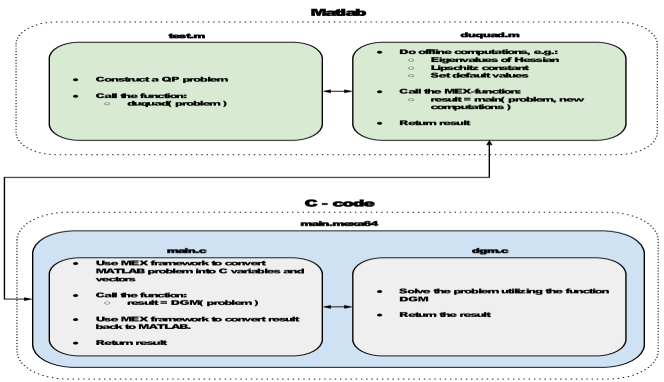
Figure 1: DuQuad workflow.

An overview of the workflow in DuQuad KwaNec:14 is illustrated in Fig. 1. A QP problem is constructed using a Matlab script called test.m. Then, the function duquad.m is called with the problem data as input and blackit is regarded as a preprocessing stage for the online optimization. The binary MEX file is called, with the original problem data and the extra blackinformation as blackan input. The main.c file of the C-code includes the MEX framework and is able to convert the MATLAB data into C format. Furthermore, the converted data gets bundled into a C “struct” and passed as blackan input to the algorithm that solves the problem using the blacktwo steps as described above.

In DuQuad blacka user can choose either algorithm IDFGM or algorithm IDGM for solving the dual problem. blackMoreover, the user can also choose the inner accuracy $\delta$ for solving the inner problem. blackIn the toolbox the default values for $\delta$ are taken as in Theorems 3.2, 3.3 and 3.4. From these theorems we conclude that the inner QP has to be solved with higher accuracy in dual fast gradient algorithm IDFGM than in dual gradient algorithm IDGM. This shows that dual gradient algorithm IDGM is robust to inexact information, while dual fast gradient algorithm IDFGM is sensitive to inexact computations, as we can also see from blackplots in Fig. 2.

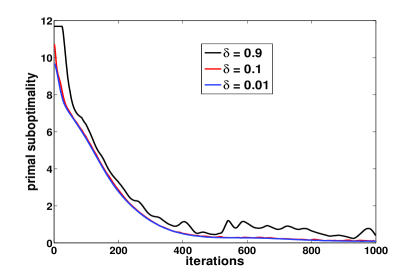
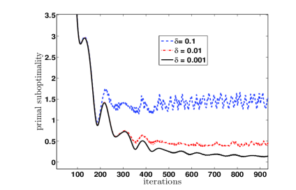
Figure 2: Sensitivity of IDGM (left) and IDFGM (right) in the average of iterates in terms of primal suboptimality w.r.t. different values of the inner accuracy $\delta$ for a QP ($n=50$ and $p=75$) with desired accuracy $\epsilon=0.01$.

Let us analyze now the computational cost per inner and outer iteration for algorithm IDFOM for solving approximately the original QP problem (38):

Inner iteration: When solving the inner problem with Nesterov’s optimal method Nes:13 , the main computational effort is done in computing the gradient of the Lagrangian $\nabla\mathcal{L}(\mathbf{u},\mathbf{x})=\mathbf{Q}\mathbf{u}+\mathbf{q}+\mathbf{G}^{T}\mathbf{x}$. In DuQuad these matrix-vector operations are implemented efficiently in C (blackthe matrices that do not change along iterations are computed once and only $\mathbf{G}^{T}\mathbf{x}$ is computed at each outer iteration). The cost for computing $\nabla\mathcal{L}(\mathbf{u},\mathbf{x})$ for general QPs is ${\cal O}(n^{2})$. However, when the matrices $\mathbf{Q}$ and $\mathbf{G}$ are sparse (e.g. network utility maximization problem) the cost ${\cal O}(n^{2})$ can be reduced substantially. The other operations in algorithm IDFOM are just vector operations and, blackhence, they are of order ${\cal O}(n)$. Thus, the dominant operation at the inner stage is the matrix-vector product.

Outer iteration: The main computational effort in the outer iteration of IDFOM is done in computing the inexact gradient of the dual function: $\tilde{\nabla}d(\mathbf{x})=\mathbf{G}\tilde{\mathbf{u}}(\mathbf{x})+\mathbf{g}.$ The cost for computing $\tilde{\nabla}d(\mathbf{x})$ for general QPs is ${\cal O}(np)$. However, when the matrix $\mathbf{G}$ is sparse, this cost can be reduced. The other operations in algorithm IDFOM are of order ${\cal O}(p)$. blackHence, the dominant operation at the outer stage is also the matrix-vector product.

Fig. 3 displays the result of profiling the code with gprof. In this simulation, a standard QP with inequality constraints, and blackwith dimensions $n=150$ and $p=225$ was solved by algorithm IDFGM. The profiling summary is listed in the order of the time spent in each file. This figure shows that most of the execution time of the program is spent on the library module math-functions.c. More exactly, the dominating function is mtx-vec-mul, which multiplies a matrix with a vector.

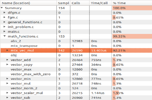
Figure 3: Profiling the code with gprof.

In conclusion, in DuQuad the main operations are the matrix-vector products. Therefore, DuQuad is adequate for solving QP problems on hardware with limited resources and capabilities, since it does not require any solver for linear systems or other complicating operations, while most of the existing solvers for QPs from the literature black(such as those implementing active set or interior point methods) require the capability of solving linear systems. On the other hand, DuQuad can be also used for solving large-scale sparse QP problems blacksince, in this case, the iterations are computationally inexpensive (only sparse matrix-vector products).

5 Numerical simulations with DuQuad

For numerical experiments, using the solver DuQuade KwaNec:14 , we blackat first consider random QP problems and then a real-time MPC controller for a self balancing robot.

5.1 Random QPs

In this section we analyze the behavior of the dual first order methods presented in this chapter and implemented in DuQuad for solving random QPs.

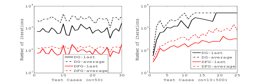
Figure 4: Number of outer iterations on random QPs for IDGM and IDFGM in primal last/average of iterates for different test cases of the same dimension (left) and of variable dimension (right).

In Fig. 4 we plot the practical number of outer iterations on random QPs of algorithms IDGM and IDFGM for different test cases of the same dimension $n=50$ (left) and for different test cases of variable dimension ranging from $n=10$ to $n=500$ (right). We blackhave choosen the accuracy $\epsilon=0.01$ and the stopping criteria is the requirement that both quantities

$$\lvert f(\mathbf{u})-f^{*}\rvert\quad\text{and}\quad\lVert[\mathbf{G}\mathbf{u}+\mathbf{g}]_{+}\rVert$$

are less than the accuracy $\epsilon$, blackwhere $f^{*}$ has been computed a priori with Matlab quadprog. From this figure we observe that the number of iterations blackis not varying much for different test cases and, also, that the number of iterations blackis mildly dependent on blackthe problem’s dimension. Finally, we observe that dual first order methods perform usually better in the primal last iterate than in the average of primal iterates.

5.2 Real-time MPC for balancing robot

In this section we use the dual first order methods presented in this chapter and implemented in DuQuad for solving a real-time MPC control problem.

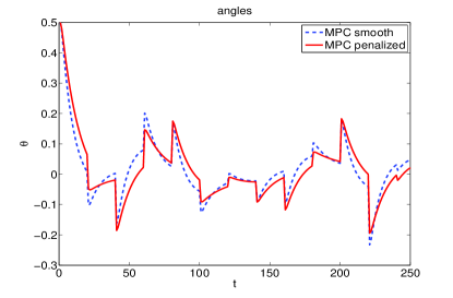
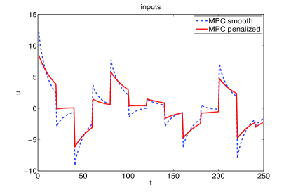
Figure 5: The MPC trajectories of the state angle (left) and input (right) for $N=10$ obtained using algorithm IDGM from DuQuad in the last iterate with accuracy $\epsilon=10^{-2}$.

We consider a simplified model for the blackself-balancing Lego mindstorm NXT extracted from Yam:08 . The model is linear time invariant and stabilizable. The continuous linear model has the states $\mathbf{x}\in\mathbb{R}^{4}$ and inputs $\mathbf{u}\in\mathbb{R}$. The states for this system are the horizontal position and speed ($h,\dot{h}$), and the angle to the vertical and the angular velocity of the robot’s body ($\theta,\dot{\theta}$). The input for the system represents the pulse-width modulaed voltage applied to both wheel motors in percentages. We discretize the dynamical system via the zero-order hold method for a sample time of $T=8\text{ms}$ to obtain the system matrices:

$$A =\begin{bmatrix}1&0.0054&-2\cdot 10^{-4}&10^{-4}\\ 0&0.4717&-0.0465&0.0211\\ 0&0.03&1.0049&0.0068\\ 0&6.0742&1.0721&0.7633\end{bmatrix},\quad B=\begin{bmatrix}0.0002\\ 0.0448\\ -0.0025\\ -0.5147\end{bmatrix}.$$

For this linear dynamical system we consider the duty-cycle percentage constraints for the inputs, i.e. $-12\leq u(t)\leq 12$, and additional constraints for the position, i.e. $-0.5\leq h\leq 0.5$, and for the body angle in degrees, i.e. $-15\leq\theta\leq 15$. For the quadratic stage cost we consider matrices: $\mathbf{Q}=\text{diag}([1\;1\;6\cdot 10^{2}\;1])$ and $\mathbf{R}=2$.

We consider two condensed MPC formulations: MPC smooth and MPC penalized, where we blackimpose additionally a penalty term $\beta(u(t)-u(t-1))^{2}$, with $\beta=0.1$, in order to get blacka smoother controller. Note that in both formulations we obtain QPs RawMay:09 . Initial state is $\mathbf{x}=[0\;0\;0.5\;-0.35]^{T}$ and we add gentle disturbances to the system at each $20$ simulation steps. In Fig. 5 we plot the MPC trajectories of the state angle and input for a prediction horizon $N=10$ obtained using algorithm IDGM in the last iterate with accuracy $\epsilon=10^{-2}$. Similar state and input trajectories are obtained using the other versions of the scheme IDFOM from DuQuad. We observe a smoother behavior for MPC with blackthe penalty term.

References

• (1) A. Beck, A. Nedić, A. Ozdaglar and M. Teboulle, An O(1/k) gradient method for network resource allocation problems, IEEE Trans. Control Network Systems, 1(1), 64–73, 2014.
• (2) A. Bemporad, M. Morari, V. Dua and E.N. Pistikopoulus, The explicit linear quadtratic regulator for constrained systems, Automatica, 38(1), 3–20, 2002.
• (3) O. Devolder, F. Glineur and Y. Nesterov, First-order methods of smooth convex optimization with inexact oracle, Mathematical Programming, 146(1-2), 37–75, 2014.
• (4) H. Ferreau, C. Kirches, A. Potschka, H. Bock and M. Diehl, qpOASES: a parametric active-set algorithm for quadratic programming, Mathematical Programming Computation, 6(4), 327–363, 2014.
• (5) J. Koshal, A. Nedić and U.V. Shanbhag, Multiuser optimization: distributed algorithms and error analysis, SIAM Journal on Optimization 21(3): 1046–1081, 2011.
• (6) S. Kvamme and I. Necoara, DuQuad User s Manual, http://acse.pub.ro/person/ion-necoara, 2014.
• (7) I. Necoara and A. Patrascu, Iteration complexity analysis of dual first order methods for convex conic programming, Technical report, UPB, 2014, http:arxiv.org.
• (8) V. Nedelcu, I. Necoara and Q. Tran Dinh, Computational complexity of inexact gradient augmented Lagrangian methods: application to constrained MPC, SIAM J. Control and Optimization, 52(5): 3109–3134, 2014.
• (9) I. Necoara and V. Nedelcu, On linear convergence of a distributed dual gradient algorithm for linearly constrained separable convex problems, Automatica, 55(5): 209—216, 2015.
• (10) I. Necoara and V. Nedelcu, Rate analysis of inexact dual first order methods: application to dual decomposition, IEEE Transactions Automatic Control, 59(5), 1232–1243, 2014.
• (11) I. Necoara, L. Ferranti and T. Keviczky, An adaptive constraint tightening approach to linear MPC based on approximation algorithms for optimization, J. Optimal Control: Applications and Methods, DOI: 10.1002/oca.2121, 1–19, 2014.
• (12) I. Necoara and J. Suykens, Application of a smoothing technique to decomposition in convex optimization, IEEE Transactions Automatic Control, 53(11), 2674–2679, 2008.
• (13) Y. Nesterov, Introductory Lectures on Convex Optimization, Kluwer, 2004.
• (14) Y. Nesterov, Smooth minimization of non-smooth functions, Mathematical Programming, 103(1), 127–152, 2005.
• (15) Y. Nesterov, Gradient methods for minimizing composite functions, Mathematical Programming, 140(1), 125–161, 2013.
• (16) A. Nedić and A. Ozdaglar, Approximate primal solutions and rate analysis for dual subgradient methods, SIAM J. Optimization, 19(4), 1757–1780, 2009.
• (17) P. Patrinos and A. Bemporad, An accelerated dual gradient-projection algorithm for embedded linear model predictive control, IEEE Transactions Automatic Control, 59(1), 18–33, 2014.
• (18) J. Rawlings and D. Mayne, Model Predictive Control: Theory and Design, Nob Hill Publishing, 2009.
• (19) C. Rao, S. Wright and J. Rawlings, Application of interior point methods to model predictive control, J. Optimization Theory Applications, 99, 723–757, 1998.
• (20) S. Richter, C. Jones and M. Morari, Computational complexity certification for real-time MPC with input constraints based on the fast gradient method, IEEE Transactions Automatic Control, 57(6), 1391–1403, 2012.
• (21) Y. Yamamoto, NXTway-GS Model-Based Design - Control of self-balancing two-wheeled robot built with LEGO Mindstorms NXT, www.pages.drexel.edu, 2008
• (22) R. Zimmerman, C. Murillo-Sanchez and R. Thomas, Matpower: steady-state operations, planning, and analysis tools for power systems research and education, IEEE Transactions Power Systems, 26(1), 12–19, 2011.
• (23) E. Wei, A. Ozdaglar and A. Jadbabaie, A distributed newton method for network utility maximization–Part I and II, IEEE Transactions Automatic Control, 58(9), 2176–2188, 2013.