The Impact of Nonlinear Structure Formation on the Power Spectrum of Transverse Momentum Fluctuations and the Kinetic Sunyaev-Zel’dovich Effect

Abstract

Cosmological transverse momentum fields, whose directions are perpendicular to Fourier wave vectors, induce temperature anisotropies in the cosmic microwave background via the kinetic Sunyaev-Zel’dovich (kSZ) effect. The transverse momentum power spectrum contains the four-point function of density and velocity fields, $\langle\delta\delta vv\rangle$. In the post-reionization epoch, nonlinear effects dominate in the power spectrum. We use perturbation theory and cosmological $N$-body simulations to calculate this nonlinearity. We derive the next-to-leading order expression for the power spectrum with a particular emphasis on the connected term that has been ignored in the literature. While the contribution from the connected term on small scales ($k>0.1~{}h~{}\rm{Mpc}^{-1}$) is subdominant relative to the unconnected term, we find that its contribution to the kSZ power spectrum at $\ell=3000$ at $z<6$ can be as large as ten percent of the unconnected term, which would reduce the allowed contribution from the reionization epoch ($z>6$) by twenty percent. The power spectrum of transverse momentum on large scales is expected to scale as $k^{2}$ as a consequence of momentum conservation. We show that both the leading and the next-to-leading order terms satisfy this scaling. In particular, we find that both of the unconnected and connected terms are necessary to reproduce $k^{2}$.

L]KS

1. Introduction

The cosmic transverse momentum field is observable in temperature fluctuations of the cosmic microwave background (CMB). The line-of-sight (LOS) component of the momentum of electrons in the ionized intergalactic medium (IGM) induces temperature fluctuations via the Doppler effect, and this is known as the kinetic Sunyaev-Zel’dovich (kSZ) effect (Zel’dovich and Sunyaev, 1969). The contribution from the longitudinal momentum field, whose direction is parallel to the wave vector, suffers from cancellation of the contributions of troughs and crests integrated along the LOS; thus, the contribution from the transverse momentum field dominates (Vishniac, 1987).

The kSZ effect is given by (Sunyaev and Zel’dovich, 1980)

$$\frac{\Delta T(\hat{\gamma})}{T}=-\int d\tau e^{-\tau}\frac{\hat{\gamma}\cdot\mathbb{v}}{c},$$ (1)

where $\hat{\gamma}$ is the LOS unit vector, $\mathbb{v}$ the peculiar velocity field, and $\tau$ the optical depth to Thomson scattering integrated through the IGM from $z=0$ to the scatterer. The differential form of $\tau$ is $d\tau=c~{}n_{e}\sigma_{\rm{T}}\left(\frac{dt}{dz}\right)dz$, where $n_{e}$ is the number density of free electrons in the IGM, and $\sigma_{\rm{T}}$ is the Thomson scattering cross section.

Equation (1) can be rewritten in the following form:

$$\frac{\Delta T}{T}(\hat{\gamma})=-\frac{\sigma_{T}\bar{n}_{e,0}}{c}\int\frac{ds}{a^{2}}~{}e^{-\tau}\mathbb{q}\cdot\hat{\gamma},$$ (2)

where $\mathbb{q}\equiv\chi\mathbb{v}(1+\delta)$ is the momentum of ionized gas, $\delta$ is the fractional mass density perturbation of the gas, $\chi\equiv n_{e}/(n_{\rm{H}}+2n_{\rm{He}})$ the ionization fraction, $\bar{n}_{e,0}=\bar{n}_{\rm{H,0}}+2\bar{n}_{\rm{He,0}}$ the mean number density of electrons at the (fully-ionized) present epoch, and $s$ the distance photons travelled from a source to the observer in comoving units.

Longitudinal momentum fields cancel out in the line-of-sight integral of Equation (2) (See Appendix A for a quantitative argument; also see Vishniac, 1987). Then, the angular power spectrum of Equation (2), $C_{\ell}$, at large multipoles is dominated by the power spectrum of the transverse momentum field, $P_{q_{\perp}}(k)$, and is given by (Vishniac, 1987)

$$C_{\ell}=\frac{1}{2}\left(\frac{\sigma_{T}\bar{n}_{e,0}}{c}\right)^{2}\int\frac{ds}{s^{2}a^{4}}e^{-2\tau}P_{q_{\perp}}\left(k=\frac{l}{s},s\right).$$ (3)

The kSZ power spectrum has been constrained by observations. The South Pole Telescope (SPT) and Atacama Cosmology Telescope (ACT) measure CMB temperature anisotropy at scales beyond the Silk damping scale ($\ell\gtrsim 3000$) where it is possible to distinguish the kSZ signal from the primary signal. The latest constraint is $D^{\rm{kSZ}}_{\ell=3000}=2.9\pm 1.3~{}\mu K^{2}$ (69% CL), where $D_{\ell}\equiv\ell(\ell+1)C_{\ell}/2\pi$ (George et al., 2015).

The measured kSZ power spectrum is the sum of contributions from the epoch of reionization (EoR) and the post-reionization epoch. The model of Shaw et al. (2012) suggests that the latter gives $D^{\rm{kSZ}}_{\ell=3000}\approx 2.0~{}\mu K^{2}$, assuming that the universe became fully ionized at $z=6$. Thus, the central value of the current measurement implies that the post-reionization kSZ signal is a factor of two greater than the EoR signal. This highlights the importance of understanding the post-reionization signal; if we mis-calculate the post-reionization signal by ten percent, the EoR signal would be mis-estimated by twenty percent. This motivates our revisiting assumptions used by the previous calculations of the post-reionization kSZ power spectrum.

Inhomogeneity in the ionization fraction during the EoR gives a large boost in the kSZ power spectrum compared to homogeneous ionization (Park et al., 2013). The physics that determines this inhomogeneity is complex, and many papers have been written on this subject, ranging from early analytical calculations (Gruzinov and Hu, 1998; Santos et al., 2003) and semi-numerical calculations using an analytical ansatz applied to $N$-body simulations (Zahn et al., 2005; McQuinn et al., 2005; Mesinger et al., 2012; Zahn et al., 2011; Battaglia et al., 2013), to fully numerical simulations that couple the cosmological structure formation with radiative transfer (Iliev et al., 2007; Park et al., 2013).

Modeling the post-reionization signal is simpler because the IGM is fully ionized and $\chi$ does not fluctuate to a good approximation. We thus need to model the density and velocity fluctuations of gas. When $\chi=1$, the momentum field is given by $\mathbb{q}=\mathbb{v}(1+\delta)$. Since the velocity field is purely longitudinal in the linear regime, the transverse momentum field, $\mathbb{q}_{\perp}$, is given by $\mathbb{q}_{\perp}=(\mathbb{v}\delta)_{\perp}$ at leading order. The power spectrum is then given by the four-point function of two densities and velocities. Schematically, it is given by $\langle qq\rangle=\langle vv\rangle\langle\delta\delta\rangle+2\langle v\delta\rangle^{2}+\langle v\delta v\delta\rangle_{c}$. The last term is called the connected four-point term, while the others are the unconnected ones.

In the previous work, the connected term has been ignored. For example, the earlier analytical studies ignore nonlinearity in density or velocity, and calculate only the unconnected terms using linear perturbation theory (Ostriker and Vishniac, 1986; Vishniac, 1987; Dodelson and Jubas, 1995; Jaffe and Kamionkowski, 1998). An analytical model of Hu (2000) is still based upon linear theory for velocity, and ignores the connected term, but replaces the linear density power spectrum with a model for the nonlinear density power spectrum by Peacock and Dodds (1996). Ma and Fry (2002) use a similar approach with a halo model for the nonlinear density power spectrum and argue that the connected term is negligible at large $k$. While we broadly agree with this conclusion, our aim is to quantify the contribution of the connected term at large $k$, and also clarify the role of the connected term in obtaining the correct small-$k$ limit of the transverse momentum power spectrum in perturbation theory.

Some of the previous “numerical” calculations of the post-reionization kSZ power spectrum (Zhang et al., 2004; Shaw et al., 2012) still rely on the above analytical model that ignores the connected term, but takes the ingredient of the model, i.e., nonlinear gas density power spectrum, from hydrodynamical simulations. Therefore, quantifying better the contribution of the connected term affects the results from the previous numerical work as well. Springel et al. (2001) and da Silva et al. (2001) computed the kSZ power spectrum directly from their simulation and did not rely on the model.

Throughout this paper, we shall assume that gas traces dark matter. This is not a great approximation: shocks in the IGM generated by structure formation heat gas to high temperatures (e.g., Cen and Ostriker, 1999), and the resulting gas pressure makes gas less clustered than dark matter particles. This effect on the kSZ power spectrum is modest at $\ell=3000$ (Shaw et al., 2012; Hu, 2000). Star formation converts gas into stars, further reducing the kSZ effect. Shaw et al. (2012) find that $D^{\rm kSZ}_{\ell=3000}$ can be suppressed by as much as 33% of the simulation without gas cooling and star formation. Our goal in this paper is to quantify the error we make by ignoring the connected four-point term in the transverse momentum power spectrum. While our dark-matter-only results cannot be extrapolated to gas, we expect that a similar conclusion would still apply to gas, at least qualitatively.

The remainder of this paper is organized as follows. In Section 2, we briefly introduce the $N$-body simulation we use in this paper. In Section 3, we review the derivation of the current nonlinear transverse momentum power spectrum model (Hu, 2000; Ma and Fry, 2002). In Section 4, we first confirm that the current model accurately approximates the unconnected term. We then show that our simulation data of the transverse momentum power spectrum exceed the model. We argue that this excess is due to the connected term, by showing that the perturbation theory calculation of the next-to-leading order terms (including the connected term) explains the excess at quasi-linear scales successfully. We also show that the connected term is essential in obtaining the correct low-$k$ limit of the transverse momentum power spectrum in perturbation theory. In Section 5, we quantify the impact of the connected term on the post-reionization kSZ power spectrum. We conclude in Section 6.

2. Simulation

We shall use a cosmological $N$-body simulation of collisionless particles using the “CubeP³M” $N$-body code (Harnois-Déraps et al., 2013). The simulation is run with $3456^{3}$ particles in a comoving box of $1~{}h^{-1}~{}{\rm Gpc}$ on a side and is started at $z=150$ using the initial condition generated using the Zel’dovich approximation and initial density power spectrum from the publicly available code CAMB (Lewis et al., 2000). This simulation was previously presented in Watson et al. (2013).

The resolution of this simulation allows us to sample on average $\sim 40$ particles per $({\rm Mpc}/h)^{3}$. This resolution allows us to avoid sampling artifacts in the velocity power spectrum up to $k\sim 1~{}h~{}\rm{Mpc}^{-1}$ (see Figure 3 of Zhang et al., 2015). We then adaptively smooth particles to a grid of $(1008)^{3}$ cells . Therefore, our simulation covers a dynamic range of $0.006\lesssim k\lesssim 1~{}h~{}\rm{Mpc}^{-1}$ in wavenumber. The background cosmology is based on the WMAP 5-year data combined with constraints from baryonic acoustic oscillations, from observations of galaxies and large-scale structures, and from high-redshift Type Ia supernovae ($\Omega_{M}=0.279,\Omega_{\Lambda}=0.721,h=0.701,\Omega_{b}=0.0462,\sigma_{8}=0.8,n_{s}=0.96$; Komatsu et al., 2009).

3. Transverse momentum power spectrum

3.1. Basics

In the post-reionization era, helium atoms are singly ionized until He II reionization occurs. We assume that hydrogen reionization finished at $z=6$ and He II reionization occurred instantaneously at $z=3$; thus, $\chi=0.93$ for $3<z<6$ and $\chi=1$ for $z\leq 3$. For the rest of the paper, we shall drop $\chi$ for notational simplicity and write $\mathbb{q}=\mathbb{v}(1+\delta)$. Therefore, the momentum power spectrum below should be rescaled by $\chi^{2}$ to yield the correct value needed for computing the kSZ power spectrum in Section 5.

We start by Fourier transforming the momentum field, $\mathbb{q}=\mathbb{v}(1+\delta)$, as

$$\mathbb{\tilde{q}(k)}=\mathbb{\tilde{v}(k)}+\int\frac{d^{3}k^{\prime}}{(2\pi)^{3}}\tilde{\delta}\mathbb{(k-k^{\prime})}\mathbb{\tilde{v}(k^{\prime})},$$ (4)

where $\tilde{\mathbb{q}}(\mathbb{k})\equiv\int d^{3}\mathbb{x}~{}e^{i\mathbb{k}\cdot\mathbb{x}}\mathbb{q}(\mathbb{x})$, etc. Then, its power spectrum is defined by

$$(2\pi)^{3}P^{ij}_{qq}(\mathbb{k_{1}})\delta_{D}(\mathbb{k_{1}}+\mathbb{k_{2}})\equiv\left<\tilde{q}^{i}(\mathbb{k_{1}})\tilde{q}^{j}(\mathbb{k_{2}})\right>$$

$$= \left<\tilde{v}^{i}(\mathbb{k_{1}})\tilde{v}^{j}(\mathbb{k_{2}})\right>+2\int\frac{d^{3}k^{\prime}}{(2\pi)^{3}}\left<\tilde{\delta}(\mathbb{k_{1}}-\mathbb{k^{\prime}})\tilde{v}^{i}(\mathbb{k^{\prime}})\tilde{v}^{j}(\mathbb{k_{2}})\right>$$

$$+ \int\frac{d^{3}k^{\prime}}{(2\pi)^{3}}\int\frac{d^{3}k^{\prime\prime}}{(2\pi)^{3}}\left<\tilde{\delta}(\mathbb{k_{1}}-\mathbb{k^{\prime}})\tilde{v}^{i}(\mathbb{k^{\prime}})\tilde{\delta}(\mathbb{k_{2}}-\mathbb{k^{\prime\prime}})\tilde{v}^{j}(\mathbb{k^{\prime\prime}})\right>,$$

where the indices, $i$ and $j$, denote the $i$’th and $j$’th components of the vector, respectively. The power spectrum of the transverse mode, $\tilde{\mathbb{q}}_{\perp}\equiv\tilde{\mathbb{q}}-\hat{\mathbb{k}}[\tilde{\mathbb{q}}\cdot\hat{\mathbb{k}}]$, is given by $P_{q_{\perp}}\equiv\Sigma_{i}P^{ii}_{qq}[1-(\hat{k}^{i})^{2}]$. In linear and quasi-linear regimes ($k\lesssim 1~{}h/\rm{Mpc}$), the velocity field is longitudinal (i.e. $\tilde{\mathbb{v}}(\mathbb{k})=\hat{\mathbb{k}}\tilde{v}$) to a good approximation, which implies that $\left<vv\right>$ and $\left<\delta vv\right>$ in Equation (LABEL:eq:Pq_brac) vanish. Figure 1 shows that the contribution to $P_{q_{\perp}}$ from $\langle\delta vv\rangle$ (diamonds) is a few orders of magnitude smaller than $\langle\delta\delta vv\rangle$ (triangles). The contribution from $\langle vv\rangle$ (not shown) is even smaller than $\langle\delta vv\rangle$ by another two orders of magnitude.

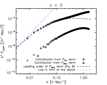
Figure 1.— Contributions to $k^{2}P_{q_{\perp}}$ from $\left<\delta vv\right>$ (diamonds) and $\langle\delta\delta vv\rangle$ (triangles) in Equation (LABEL:eq:Pq_brac) measured from our simulation at $z=0$. The red triangles show negative values. The dashed line shows the lowest order calculation for the $\left<\delta\delta vv\right>$ term, while the dotted line shows its low-$k$ limit given in Equation (11).

Keeping only the last term in Equation (LABEL:eq:Pq_brac), we obtain

$$P_{q_{\perp}}(k) = \int\frac{d^{3}k^{\prime}}{(2\pi)^{3}}\int\frac{d^{3}k^{\prime\prime}}{(2\pi)^{3}}[\hat{\mathbb{k^{\prime}}}\cdot\hat{\mathbb{k^{\prime\prime}}}-(\hat{\mathbb{k}}\cdot\hat{\mathbb{k^{\prime}}})(\hat{\mathbb{k}}\cdot\hat{\mathbb{k^{\prime\prime}}})]$$ (6)

$$P_{\delta\delta vv}(\mathbb{k}-\mathbb{k^{\prime}},-\mathbb{k}-\mathbb{k^{\prime\prime}},\mathbb{k^{\prime}},\mathbb{k^{\prime\prime}}),$$

where $P_{\delta\delta vv}$ is defined by

$$(2\pi)^{3}P_{\delta\delta vv}(\mathbb{k_{1}},\mathbb{k_{2}},\mathbb{k_{3}},\mathbb{k_{4}})\delta_{D}(\mathbb{k_{1}}+\mathbb{k_{2}}+\mathbb{k_{3}}+\mathbb{k_{4}})$$ (7)

$$\equiv \left<\tilde{\delta}(\mathbb{k_{1}})\tilde{\delta}(\mathbb{k_{2}})\tilde{v}^{i}(\mathbb{k_{3}})\tilde{v}^{j}(\mathbb{k_{4}})\right>.$$

3.2. Linear Regime

In the linear regime, we consider only the first order terms of $\tilde{\delta}$’s and $\tilde{v}$’s in $\left<\delta\delta vv\right>$. Then, Gaussianity of linear $v$ and $\delta$ fields yields

$$\left<\tilde{\delta}(\mathbb{k_{1}}-\mathbb{k^{\prime}})\tilde{v}^{i}(\mathbb{k^{\prime}})\tilde{\delta}(\mathbb{k_{2}}-\mathbb{k^{\prime\prime}})\tilde{v}^{j}(\mathbb{k^{\prime\prime}})\right>$$ (8)

$$= \left<\tilde{\delta}(\mathbb{k_{1}}-\mathbb{k^{\prime}})\tilde{v}^{i}(\mathbb{k^{\prime}})\right>\left<\tilde{\delta}(\mathbb{k_{2}}-\mathbb{k^{\prime\prime}})\tilde{v}^{j}(\mathbb{k^{\prime\prime}})\right>$$

$$+ \left<\tilde{\delta}(\mathbb{k_{1}}-\mathbb{k^{\prime}})\tilde{\delta}(\mathbb{k_{2}}-\mathbb{k^{\prime\prime}})\right>\left<\tilde{v}^{i}(\mathbb{k^{\prime}})\tilde{v}^{j}(\mathbb{k^{\prime\prime}})\right>$$

$$+ \left<\tilde{\delta}(\mathbb{k_{1}}-\mathbb{k^{\prime}})\tilde{v}^{j}(\mathbb{k^{\prime\prime}})\right>\left<\tilde{\delta}(\mathbb{k_{2}}-\mathbb{k^{\prime\prime}})\tilde{v}^{i}(\mathbb{k^{\prime}})\right>.$$

The first term in the above vanishes and the other terms lead to (Ma and Fry, 2002)

$$P_{q_{\perp}}(k,z)=\int\frac{d^{3}k^{\prime}}{(2\pi)^{3}}(1-{\mu^{\prime}}^{2})\left[\frac{1}{{k^{\prime}}^{2}}P_{\delta\delta}(|\mathbb{k}-\mathbb{k^{\prime}}|)P_{\theta\theta}(k^{\prime})\right.$$

$$\left.\qquad\qquad\qquad\qquad-\frac{1}{|\mathbb{k}-\mathbb{k^{\prime}}|^{2}}P_{\delta\theta}(|\mathbb{k}-\mathbb{k^{\prime}}|)P_{\delta\theta}(k^{\prime})\right],$$ (9)

where $\theta\equiv\nabla\cdot\mathbb{v}$.

The linear velocity is related to the linear density by $\tilde{\theta}=\dot{a}f\tilde{\delta}$, where $f\equiv d\ln\delta/d\ln a$ and $a(t)$ is the Robertson-Walker scale factor. This gives the lowest order (LO) expression as (Vishniac, 1987)

$$P^{\rm{LO}}_{q_{\perp}}(k,z) = \dot{a}^{2}f^{2}\int\frac{d^{3}k^{\prime}}{(2\pi)^{3}}P^{lin}_{\delta\delta}(|\mathbb{k}-\mathbb{k^{\prime}}|,z)P^{lin}_{\delta\delta}(k^{\prime},z)$$ (10)

$$\qquad\qquad\times\frac{k(k-2k^{\prime}\mu^{\prime})(1-{\mu^{\prime}}^{2})}{{k^{\prime}}^{2}(k^{2}+{k^{\prime}}^{2}-2kk^{\prime}\mu^{\prime})},$$

where $P^{lin}_{\delta\delta}$ is the linear matter density power spectrum. A similar derivation for the power spectrum of the sum of longitudinal and transverse momentum fields is presented in Park (2000).

Taking $k\rightarrow 0$ limit of Equation (10), we find

$$P^{\rm{LO}}_{q_{\perp}}(k,z)\to\frac{8}{15}\dot{a}^{2}f^{2}k^{2}\int\frac{dk^{\prime}}{(2\pi)^{2}}\frac{{[P^{lin}_{\delta\delta}(k^{\prime},z)]^{2}}}{{k^{\prime}}^{2}}.$$ (11)

The $k$ dependence of $P^{\rm{LO}}_{q_{\perp}}$ is thus given simply by $k^{2}$, which is independent of cosmology or the initial power spectrum. Similarly, the second order term (2nd term in the r.h.s. of Eq. A10) of the longitudinal mode also goes as $k^{2}$ in the low-$k$ limit:

$$P^{\rm{(2)}}_{q_{\parallel}}(k,z)\to\frac{7}{15}\dot{a}^{2}f^{2}k^{2}\int\frac{dk^{\prime}}{(2\pi)^{2}}\frac{{[P^{lin}_{\delta\delta}(k^{\prime},z)]^{2}}}{{k^{\prime}}^{2}}.$$ (12)

We shall discuss the physical origin of this dependence in Section 4.2.

We use CAMB to compute $P_{\delta\delta}^{lin}$. The dashed line in Figure 1 shows $P^{\rm{LO}}_{q_{\perp}}$ at $z=0$, while the dotted line shows the low-$k$ limit (Eq. 11).

Figure 2.— Ratios of various models for $P_{q_{\perp}}$ to $P_{q_{\perp}}$ directly measured from the simulation at $z=0$ (upper left), $z=1$ (upper right), $z=2$ (lower left) and $z=5.5$ (lower right). The models include the Standard expression (Eq. 13) with $P^{nl}_{\delta\delta}$ from the simulation (squares), the unconnected term (Eq. 3.2) with $P_{\delta\delta}$, $P_{\delta\theta}$ and $P_{\theta\theta}$ from the simulation (crosses), and the connected term calculated from perturbation theory added to the crosses (triangles). The vertical dotted line denotes the wavenumber beyond which the perturbation theory fails to model nonlinearity precisely according to Jeong and Komatsu (2006) and our data. At $z=5.5$, that wavenumber is out of the plotting range and not shown in the figure.

3.3. Nonlinear Regime

As Figure 1 shows, nonlinear contributions to $P_{q_{\perp}}$ become dominant over the LO contribution at $k\gtrsim 0.2~{}h/\rm{Mpc}$ at $z=0$, in agreement with the previous work (Hu, 2000; Ma and Fry, 2002). The current popular model of the post-reionization kSZ signal uses an approximate expression for the transverse momentum power spectrum due to Hu (2000), which replaces one of $P_{\delta\delta}^{lin}$ in Equation (10) with the nonlinear power spectrum, $P_{\delta\delta}^{nl}$:

$$P^{\rm{S}}_{q_{\perp}}(k,z) = \dot{a}^{2}f^{2}\int\frac{d^{3}k^{\prime}}{(2\pi)^{3}}P_{\delta\delta}^{nl}(|\mathbb{k}-\mathbb{k^{\prime}}|,z)P^{lin}_{\delta\delta}(k^{\prime},z)$$ (13)

$$\qquad\qquad\times\frac{k(k-2k^{\prime}\mu^{\prime})(1-{\mu^{\prime}}^{2})}{{k^{\prime}}^{2}(k^{2}+{k^{\prime}}^{2}-2kk^{\prime}\mu^{\prime})}.$$

This model modifies the second term in the square bracket of Equation (3.2) in the following way:

$$P_{\delta\theta}(|\mathbb{k}-\mathbb{k}^{\prime}|)P_{\delta\theta}(k^{\prime})=P_{\delta\delta}(|\mathbb{k}-\mathbb{k}^{\prime}|)P_{\theta\theta}(k^{\prime}).$$ (14)

This holds in the linear regime, and the entire term vanishes in the large $k$ regime due to the pre-factor, $|\mathbb{k}-\mathbb{k^{\prime}}|^{-2}$. In addition, the model approximates the velocity power spectrum by linear theory, i.e., $P_{\theta\theta}=\dot{a}^{2}f^{2}P^{lin}_{\delta\delta}$. In this way, the model avoids having to model the velocity power spectrum and the density-velocity cross power spectrum, which is relatively poorly understood. We shall refer to this model as the Standard model (hence the superscript “S” in Eq. 13) in this paper.

However, Equation (3.2), which the Standard model aims to model, is not the full expression for $P_{q_{\perp}}$ because it neglects the contribution from the connected term, $\langle\delta v\delta v\rangle_{c}$. In the nonlinear regime, nonlinear growth makes both $\delta$ and $v$ non-Gaussian, and thus there is no reason to think that the connected four-point term is negligible. We shall quantify the importance of this term in detail in Section 4.2.

4. Revisiting the Standard Model for the Effect of Nonlinearity on the Transverse Momentum Power Spectrum

4.1. Unconnected Term

In this section, we revisit accuracy of Equation (13). As noted above, this model is an approximation for the unconnected term (Eq. 3.2). Therefore, it, by design, does not take into account the connected term.

We test whether Equation (13) successfully approximates Equation (3.2) by evaluating it using the density power spectrum from the simulation, i.e., $P^{nl}_{\delta\delta}=P^{sim}_{\delta\delta}$, and compare it with Equation (3.2) using $P_{\delta\delta}$, $P_{\delta\theta}$, and $P_{\theta\theta}$ from the simulation.

In Figure 2, we show the ratios of Equation (13) (squares) and Equation (3.2) (crosses) to $P_{q_{\perp}}$ measured directly from the simulation. At $0.2\lesssim k\lesssim 0.5~{}h~{}\rm{Mpc}^{-1}$ at $z=0$ (top left panel), the Standard model reproduces the unconnected term with high accuracy ($\sim 2\%$ level). However, the Standard model overestimates the unconnected term at larger $k$, reaching $\sim 5\%$ level at $k\sim 1~{}h~{}\rm{Mpc}^{-1}$. We attribute this error to the linear velocity assumption overestimating magnitudes of velocity modes. In the high-$k$ limit, Equation (3.2) converges to (Hu, 2000)

$$P_{q_{\perp}}(k)=\frac{2}{3}P_{\delta\delta}(k)v_{rms}^{2}(k),$$ (15)

where $v_{rms}^{2}(k)=\int_{k^{\prime}\leq k}\frac{d^{3}k^{\prime}}{(2\pi)^{3}}P_{vv}(k^{\prime})$ is the velocity dispersion. Nonlinear correction makes the velocity power spectrum in the relevant $k$ range smaller than the linear velocity power spectrum (see, e.g., Figure 1 of Pueblas and Scoccimarro, 2009); thus, linear theory overestimates $v_{rms}^{2}$. This effect becomes smaller at higher redshifts, as shown in the other panels of Figure 2.

We find that both Equation (3.2) and (13) underestimate $P_{q_{\perp}}$ significantly compared to $P_{q_{\perp}}$ measured directly from the simulation. The underestimation decreases monotonically with redshift: $12-25$% over $k=0.2-1.5~{}h~{}{\rm Mpc}^{-1}$ at $z=0$; $7-23$% at $z=1$; $5-18$% at $z=2$; and a few to 5% at $z=5.5$. Thus, this is likely related to the development of nonlinear structure formation.

4.2. Connected Term

To show that the connected term is the likely explanation for the difference between the simulation data and the models that ignore the connected term, we calculate the connected term using perturbation theory. Since the connected term vanishes in linear theory, we must go to the next-to-leading order perturbation theory, such as the standard “one-loop” perturbation theory (Bernardeau et al., 2002). This theory allows us to extend validity of analytic solutions for Fourier modes of density and velocity fields down to weakly nonlinear scales, e.g., in $k\lesssim 0.3~{}h~{}\rm{Mpc}^{-1}$ at $z\sim 1$ and in wider wavenumbers at higher redshifts (Jeong and Komatsu, 2006). We also confirm that the density power spectrum from our simulation data supports their findings. We derive the explicit expressions for the connected (Eq. B16) and unconnected terms (Eq. C) in Appendix B and C, and show them in the dotted and dashed lines in Figure 3, respectively.

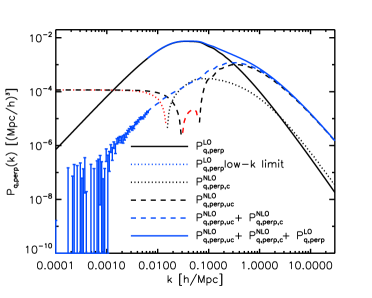
Figure 3.— $P_{q_{\perp}}$ at $z=0$ from the next-to-leading order unconnected term (black dashed), connected term (black dotted), the sum of the two next-to-leading order terms (blue dashed), and the total sum of the leading and next-to-leading order terms (blue solid). The red color shows negative values. The error bars show the uncertainty of the Monte-Carlo integration for $k<0.01~{}h~{}\rm{Mpc}^{-1}$. The solid line shows the LO term (Eq. 10), while the blue dotted line shows its low-$k$ limit (Eq. 11).

We find that each of the unconnected and connected terms does not vanish in the low-$k$ limit on its own. Instead, they converge to a constant value with opposite signs. This constant can be obtained by taking $k\to 0$ limit of Equation (B16):

$$P_{q_{\perp},c}|_{k\rightarrow 0} = \frac{16}{49}\int\frac{d^{3}k^{\prime}}{(2\pi)^{3}}\int\frac{d^{3}k^{\prime\prime}}{(2\pi)^{3}}\frac{[1-(\hat{\mathbb{k}}\cdot\hat{\mathbb{k^{\prime}}})(\hat{\mathbb{k}}\cdot\hat{\mathbb{k^{\prime\prime}}})]}{k^{\prime}k^{\prime\prime}}$$ (16)

$$\times P(\mathbb{k^{\prime}})P(\mathbb{k^{\prime}}+\mathbb{k^{\prime\prime}})P(\mathbb{k^{\prime\prime}})\left(\frac{(1-\mu^{2}){k^{\prime\prime}}{k^{\prime}}}{(\mathbb{k^{\prime}}+\mathbb{k^{\prime\prime})}^{2}}\right)^{2}.~{}~{}~{}~{}~{}$$

The sum of the two terms, however, yields a physical result that remains positive and decays toward lower $k$. The cancellation of two large numbers introduces an uncertainty in our numerical integration using the Monte Carlo method. Within the uncertainty, the result is consistent with $k^{2}$ scaling, which is the same as the scaling of the LO expression given by Equation (11). This calls for a physical explanation; namely, what is the physical origin of the $k^{2}$ scaling in the low-$k$ limit of the transverse momentum power spectrum, which is independent of cosmology or the initial power spectrum?

Figure 4.— Angular power spectrum of the kSZ effect. (Left) $dC_{\ell=3000}/ds$, which shows the contribution to $C_{\ell}$ at $\ell=3000$ from a given comoving distance. The horizontal axis shows redshifts such that it is linear in the comoving distance. The top label shows the contributing wavenumber to the kSZ signal, $\ell/s(z)$. The discontinuity at $z=3$ is due to the instantaneous helium reionization. The solid line shows the Standard kSZ model (Eq. 13) with the HALOFIT density power spectrum, the dashed line shows the next-to-leading order connected term from perturbation theory, and the dotted line shows the LO contribution (Eq. 10). We also show the simulation results at $z=0.5$, 1, and 2: the diamonds show Equation (13) with the nonlinear density power spectrum from the simulation, while the crosses use the total simulation momentum power spectrum minus the diamonds. (Right) $D_{\ell}=\ell(\ell+1)C_{\ell}/(2\pi)$. The dash-dotted line shows the primary CMB temperature power spectrum, while the other lines show the same cases as in the left panel.

As shown by Mercolli and Pajer (2014), this is a consequence of momentum conservation. In short, the argument goes as follows. Suppose that we have a uniform distribution of matter particles with no initial momentum or density fluctuation, and displace these particles with velocities $\mathbb{v}_{i}$ (where $i$ is a particle ID) in a momentum-conserving manner. In this way, we have removed the effect of the initial condition, and can focus only on the effect of the subsequent evolution of particle’s motion. Fourier transform of momentum of the displaced particles is given by $\mathbb{q}(\mathbb{k})=\sum_{i}m_{i}\mathbb{v}_{i}\exp(-i\mathbb{k}\cdot x_{i})$, and the low-$k$ limit is $\mathbb{q}(\mathbb{k})=\sum_{i}m_{i}\mathbb{v}_{i}(1-i\mathbb{k}\cdot\mathbb{x}_{i}+\dots)$. The first term vanishes by momentum conservation, giving $\mathbb{q}(\mathbb{k})={\cal O}(k)$; hence the power spectrum of momentum fields is proportional to $k^{2}$. This argument applies to both the longitudinal and transverse momentum fields. As we have found, the connected term is necessary for obtaining the correct low-$k$ limit at the next-to-leading order in perturbation theory.

5. Implication for the Post-reionization kSZ angular power spectrum

In the high-$k$ regime, the connected term is of order ten percent of the unconnected term, which brings the predicted $P_{q_{\perp}}$ into better agreement with the simulation, as shown by the triangles in Figure 2. Thus, the underestimation is now much reduced to $2-18$% over $k=0.2-1.5~{}h~{}{\rm Mpc}^{-1}$ at $z=0$; $2-18$% at $z=1$; $2-14$% at $z=2$; and a few percent at $z=5.5$. For each redshift, we mark in the figure roughly the wavenumber that the next-to-leading order (“one-loop”) calculation of perturbation theory becomes inaccurate for the density fluctuations according to Jeong and Komatsu (2006) and our data. The remaining differences beyond that wavenumber are likely due to inaccuracy of perturbation theory calculation, whereas the agreement at 2% level at small $k$ supports our conclusion that the connected term is necessary for accurate modeling of the transverse momentum power spectrum.

We use Equation (3) to calculate the observable CMB angular power spectrum of kSZ, $C_{\ell}$. In the left panel of Figure 4, we show $dC_{\ell=3000}/ds$, which is the contribution to the kSZ signal at $\ell=3000$ per comoving distance from the observer. The area under each curve gives the total $C_{\ell}$, which is shown in the right panel. The dotted line shows the LO calculation (Eq. 10). The solid line and the diamonds show the Standard kSZ model (Eq. 13) with the nonlinear matter density power spectrum computed using the HALOFIT code (Smith et al., 2003) and the simulation (i.e., the square symbols in Figure 2), respectively. We cannot calculate the kSZ contribution at $z<0.5$ in our simulation because the contributing wavenumber is beyond the resolution limit of our simulation ($k\sim 2~{}h~{}\rm{Mpc}^{-1}$). The disagreement between the two at $z=0.5$ is due to the disagreement between the HALOFIT power spectrum and our simulation at $k\gtrsim 1~{}h~{}\rm{Mpc}^{-1}$, which is also due to the resolution limit of the simulation.

The dashed line shows the next-to-leading order connected moment contribution. We also estimate the connected term contribution in our simulation by subtracting the diamonds from the total transverse momentum power spectrum measured from the simulation. The simulation at $z=1$ suggests about a factor of 3 larger effect than the next-to-leading order perturbation theory. The interpretation of the difference at $z=0.5$ is difficult because of the disagreement between the diamond and the solid line; however, if we assume that the resolution of the simulation affects the unconnected and connected terms in the same way, then the simulation at $z=0.5$ suggests about a factor of three larger effect than perturbation theory. This is expected because the kSZ signal receives contributions from $k\gtrsim 1~{}h~{}\rm{Mpc}^{-1}$ where the next-to-leading order calculation is insufficient to capture nonlinearity (see the triangles in Figure 2). The difference decreases as $z$ increases, as expected from development of nonlinear structure formation. Taking into account this extra nonlinearity above perturbation theory, we estimate that the connected term contribution to $C_{\ell}$ at $\ell=3000$ is at least ten percent of the unconnected term.

6. Summary and Conclusion

We have reexamined the currently popular model of the transverse dark matter momentum power spectrum (Eq. 13) used in the previous calculation of the post-reionization kSZ power spectrum (e.g., Shaw et al., 2012). We find that the current model reproduces the contribution of the unconnected term (Eq. 3.2) well. However, this model ignores the contribution from the connected term that arises in the nonlinear regime. Using both perturbation theory and cosmological $N$-body simulation, we show that the contribution from the connected term adds a significant additional power, especially at larger $k$ at lower $z$ (Figure 2). This is consistent with the expectation from nonlinear structure formation.

We estimate that the contribution of the connected term to the kSZ angular power spectrum at $\ell=3000$ is ten percent of the unconnected term. This is the term that needs to be added to the calculation of Shaw et al. (2012), assuming that a similar correction is necessary for the momentum power spectrum of gas. In light of the current observational constraint ($D^{\rm kSZ}_{\ell=3000}=2.9~{}\mu K^{2}$) and the post-reionization kSZ model of Shaw et al. (2012) ($D^{{\rm kSZ},z<6}_{\ell=3000}=2.0~{}\mu K^{2}$), adding ten percent to the post-reionization kSZ signal would imply a twenty percent less kSZ signal from the EoR. The semi-numerical model of Battaglia et al. (2013) implies that such a change in the reionization kSZ signal would result in a twenty percent increase in the redshift at which the mean ionized fraction of the universe reached 50%, or ten percent shorter duration of reionization, $\Delta z$. Park et al. (2013), however, show that reionization simulations based upon radiative transfer and $N$-body simulation can yield a more extended duration of the reionization epoch than these semi-numerical models predict, so this quantitative conclusion about the constraint from changing the kSZ upper limit from the EOR on the duration of reionization may need to be revised to take account of such extended reionization.

Finally, we have shown that both the LO and next-to-leading order perturbation theory calculations give $P_{q_{\perp}}\propto k^{2}$ in the low-$k$ limit, independent of cosmology or the initial power spectrum. This behavior is consistent with momentum conservation.

7. Acknowledgment

Authors thank Ilian T. Iliev for generating and storing the cosmological $N$-body simulation data used in this work. PRS was supported in part by U.S. NSF grant AST-1009799, NASA grant NNX11AE09G, NASA/JPL grant RSA Nos. 1492788 and 1515294, and supercomputer resources from NSF XSEDE grant TG-AST090005 and the Texas Advanced Computing Center (TACC) at the University of Texas at Austin. JK was supported by the Australian Research Council Centre of Excellence for All-sky Astrophysics (CAASTRO), through project number CE110001020. YM was supported by the Labex ILP (reference ANR- 10-LABX-63) part of the Idex SUPER, and received financial state aid managed by the Agence Nationale de la Recherche, as part of the programme Investissements d’avenir under the reference ANR-11-IDEX-0004-02.

Appendix A kSZ effect from Longitudinal Modes

Rewriting Equation (2) in terms of Fourier mode of $\mathbb{q}$ gives

$$\frac{\Delta T}{T}(\hat{\gamma})=-\frac{\sigma_{T}n_{e,0}}{c}\int\frac{ds}{a(s)^{2}}e^{-\tau}\int\frac{d^{3}k}{(2\pi)^{3}}[\hat{\gamma}\cdot\tilde{\mathbb{q}}(\mathbb{k},s)]e^{-i\mathbb{k}\cdot(s\hat{\gamma})}.$$ (A1)

Here, the momentum vector in Fourier space, $\tilde{\mathbb{q}}$, can be decomposed into the longitudinal mode, $\tilde{q}_{\parallel}\equiv\tilde{\mathbb{q}}\cdot\hat{k}$, and the transverse component, $\tilde{q}_{\perp}\equiv|\tilde{\mathbb{q}}-\hat{k}(\tilde{\mathbb{q}}\cdot\hat{k})|$, to give

$$\frac{\Delta T}{T}(\gamma)=-\frac{\sigma_{T}n_{e,0}}{c}\int\frac{ds}{a(s)^{2}}e^{-\tau}\int\frac{d^{3}k}{(2\pi)^{3}}[x\tilde{q}_{\parallel}+\cos(\phi_{\hat{q}}-\phi_{\hat{\gamma}})(1-x^{2})^{1/2}\tilde{q}_{\perp}(\mathbb{k},s)]e^{-iksx},$$ (A2)

where $x\equiv\hat{k}\cdot\hat{\gamma}$.

In this section, we shall derive the angular power spectrum of $q_{\parallel}$ term. The derivation given here parallels that for the transverse mode given in Appendix of Park et al. (2013). Spherical-harmonics decomposition of $q_{\parallel}$ term in the above equation is,

$$a_{\ell m} = \int d^{2}\hat{\gamma}Y^{m*}_{\ell}(\hat{\gamma})\frac{\Delta T}{T}(\hat{\gamma})$$ (A3)

$$= -\frac{\sigma_{T}n_{e,0}}{c}\int d^{2}\hat{\gamma}Y^{m*}_{\ell}(\hat{\gamma})\int\frac{ds}{a(s)^{2}}e^{-\tau}\int\frac{d^{3}k}{(2\pi)^{3}}x\tilde{q_{\parallel}}(\mathbb{k},s)e^{-iksx}$$

$$= \int\frac{d^{3}k}{(2\pi)^{3}}f_{\ell m}(\mathbb{k})$$

where

$$f_{\ell m}(\mathbb{k}) \equiv \int d^{2}\hat{\gamma}Y^{m*}_{\ell}(\hat{\gamma})\int\frac{ds}{a(s)^{2}}e^{-\tau}x\tilde{q}_{\parallel}(\mathbb{k},s)e^{-iksx}$$ (A4)

$$= \int d^{2}\hat{\gamma}Y^{m*}_{\ell}(\hat{\gamma})\int\frac{ds}{a(s)^{2}}e^{-\tau}x\tilde{q}_{\parallel}(\mathbb{k},s)\times 4\pi\sum_{LM}(-i)^{L}j_{L}(ks)Y^{M}_{L}(\hat{\gamma})Y^{M*}_{L}(\hat{k}).$$

Here, we choose a coordinate system that $\hat{k}=\hat{z}$, thereby simplifying $Y^{M*}_{L}(\hat{k})$ to $Y^{M*}_{L}(\hat{z})=\delta_{M0}\sqrt{\frac{2L+1}{4\pi}}$. Then,

$$f_{\ell m}(k\hat{z}) = \sqrt{4\pi}\int\frac{ds}{a(s)^{2}}e^{-\tau}\tilde{q}_{\parallel}(\mathbb{k},s)\sum_{L}(-i)^{L}j_{L}(ks)\int d^{2}\hat{\gamma}Y^{0}_{L}(\hat{\gamma})\cos{\theta}Y^{m*}_{\ell}(\hat{\gamma})$$ (A5)

$$= \sqrt{\frac{16\pi^{2}}{3}}\int\frac{ds}{a(s)^{2}}e^{-\tau}\tilde{q}_{\parallel}(\mathbb{k},s)\sum_{L}(-i)^{L}j_{L}(ks)\int d^{2}\hat{\gamma}Y^{0}_{L}(\hat{\gamma})Y^{0}_{1}(\hat{\gamma})Y^{m*}_{\ell}(\hat{\gamma})$$

where $\theta$ is the azimuthal angle of $\hat{\gamma}$ in the coordinate system of our choice. Also, we have used the fact that $Y^{0}_{1}(\theta,\phi)=\frac{1}{2}\sqrt{\frac{3}{\pi}}\cos{\theta}$.

The integral over $\hat{\gamma}$ can be given in terms of the Clebsch-Gorden coefficient:

$$\int d^{2}\hat{\gamma}Y^{0}_{L}(\hat{\gamma})Y^{0}_{1}(\hat{\gamma})Y^{m*}_{\ell}(\hat{\gamma})=\sqrt{\frac{3(2\ell+1)}{4\pi(2L+1)}}C_{\ell 1}(L,0;m,0)C_{\ell 1}(L,0;0,0)\delta_{0,m}.$$ (A6)

In this case, the relevant ones are

$$C_{\ell 1}(\ell+1,0;0,0)=\sqrt{\frac{\ell+1}{2\ell+1}},~{}C_{\ell 1}(\ell,0;0,0)=0,~{}C_{\ell 1}(\ell-1,0;0,0)=\sqrt{\frac{\ell}{2\ell+1}},$$ (A7)

and, they give

$$f_{\ell,m=0}(k\hat{z}) = \sqrt{4\pi(2\ell+1)}\int\frac{ds}{a(s)^{2}}e^{-\tau}\tilde{q}_{\parallel}(\mathbb{k},s)\sum_{L}(-i)^{L}j_{L}(ks)\times C_{\ell 1}(L,0;0,0)C_{\ell 1}(L,0;0,0)$$

$$= (-i)^{\ell+1}\sqrt{4\pi(2\ell+1)}\int\frac{ds}{a(s)^{2}}e^{-\tau}\left[\frac{\ell+1}{2\ell+1}j_{\ell+1}(ks)-\frac{\ell}{2\ell+1}j_{\ell-1}(ks)\right]$$

$$= (-i)^{\ell+1}\sqrt{\pi(2\ell+1)}\int\frac{ds}{a(s)^{2}}e^{-\tau}\frac{j_{\ell}(ks)}{ds};$$

$$f_{\ell,m\neq 0}(k\hat{z}) = 0.$$ (A8)

Isotropy of the universe allows us to generalize above for $f_{\ell m}(\mathbb{k})$ with any $\hat{\mathbb{k}}$.

Figure 5.— Angular power spectrum of the kSZ effect from the transverse momentum field (solid) and the longitudinal momentum field (dot-dashed) in second order. The short-dashed and dotted lines denote contributions from the 1st and 2nd order terms in the longitudinal mode, respectively. The long-dashed line shows the primary CMB power spectrum.

Then, we obtain the final expression for the angular power spectrum:

$$C^{\parallel}_{\ell}=\left(\frac{n_{e}\sigma_{T}}{c}\right)^{2}\frac{1}{\pi}\int{\frac{ds}{a(s)^{2}}}\int{\frac{ds^{\prime}}{a(s^{\prime})^{2}}}\int dk\frac{dj_{\ell}(ks)}{ds}\frac{dj_{\ell}(ks^{\prime})}{ds^{\prime}}\sqrt{P_{q_{\parallel}}(k,z(s))P_{q_{\parallel}}(k,z(s^{\prime}))}.$$ (A9)

We can show that $C^{\parallel}_{\ell}$ is much smaller than $C_{\ell}$ in Equation (3) using $P_{q_{\perp}}$ and $P_{q_{\parallel}}$ from the 2nd order calculation. For $P_{q_{\perp}}$, 2nd order is the leading order, and the expression (Eq. 10) and the derivation are shown in Section 3. For $P_{q_{\parallel}}$, the 2nd order terms follows the 1st order term:

$$P_{q_{\parallel}}(k,z)=\left(\frac{\dot{a}f}{k}\right)^{2}P^{lin}_{\delta\delta}(k,z)+\dot{a}^{2}f^{2}\int\frac{d^{3}k^{\prime}}{(2\pi)^{3}}P^{lin}_{\delta\delta}(|\mathbb{k}-\mathbb{k^{\prime}}|,z)P^{lin}_{\delta\delta}(\mathbb{k^{\prime}},z)\frac{k\mu^{\prime}(k\mu^{\prime}-k^{\prime}{\mu^{\prime}}^{2}+k^{\prime})}{{k^{\prime}}^{2}(k^{2}+{k^{\prime}}^{2}-2kk^{\prime}\mu^{\prime})}$$ (A10)

(Ma and Fry, 2002). Here, $P^{lin}_{\delta\delta}$ is the linear density power spectrum and $\mu^{\prime}=\hat{\mathbb{k}}\cdot\hat{\mathbb{k^{\prime}}}$.

In Figure 5, we show the 2nd order calculation of kSZ angular power spectrum from longitudinal and transverse modes. 1st order term in the longitudinal modes dominates at $\ell\lesssim 100$, but diminishes rapidly in increasing $\ell$ as argued in Vishniac (1987). At $\ell\gtrsim 3000$ where the primary CMB vanishes to the level of allowing kSZ signal to be measured, the longitudinal mode contribution is below the transverse mode contribution by four orders of magnitude or more. Based on this comparison, we do not expect the longitudinal modes to be important even to a percent level and we shall ignore their contribution in this work.

Appendix B Connected Term in Perturbation Theory

We take the third term in Equation (6) and express it in terms of $\theta\equiv\nabla\cdot\mathbb{v}$, which is equivalent to say $\tilde{\mathbb{v}}(\mathbb{k})=i(\hat{\mathbb{k}}/k)\tilde{\theta}$:

$$P_{q_{\perp},c} = \int\frac{d^{3}k^{\prime}}{(2\pi)^{3}}\int\frac{d^{3}k^{\prime\prime}}{(2\pi)^{3}}[\hat{\mathbb{k^{\prime}}}\cdot\hat{\mathbb{k^{\prime\prime}}}-(\hat{\mathbb{k}}\cdot\hat{\mathbb{k^{\prime}}})(\hat{\mathbb{k}}\cdot\hat{\mathbb{k^{\prime\prime}}})]P_{\delta\delta vv,c}(\mathbf{k}-\mathbf{k^{\prime}},-\mathbf{k}-\mathbf{k^{\prime\prime}},\mathbf{k^{\prime}},\mathbf{k^{\prime\prime}})$$ (B1)

$$= -(\dot{a}f)^{2}\int\frac{d^{3}k^{\prime}}{(2\pi)^{3}}\int\frac{d^{3}k^{\prime\prime}}{(2\pi)^{3}}\left[\frac{\hat{\mathbb{k^{\prime}}}\cdot\hat{\mathbb{k^{\prime\prime}}}-(\hat{\mathbb{k}}\cdot\hat{\mathbb{k^{\prime}}})(\hat{\mathbb{k}}\cdot\hat{\mathbb{k^{\prime\prime}}})}{k^{\prime}k^{\prime\prime}}\right]P_{\delta\delta\theta\theta,c}(\mathbf{k}-\mathbf{k^{\prime}},-\mathbf{k}-\mathbf{k^{\prime\prime}},\mathbf{k^{\prime}},\mathbf{k^{\prime\prime}}).$$

Let us derive $P_{\delta\delta\theta\theta,c}$ using perturbation theory. We begin with the next-to-leading order expression for the full expression for $P_{\delta\delta\theta\theta}$ that includes the unconnected terms:

$$(2\pi)^{3}P_{\delta\delta\theta\theta}(\mathbf{k_{1}},\mathbf{k_{2}},\mathbf{k_{3}},\mathbf{k_{4}})\delta_{\rm D}(\mathbf{k_{1}}+\mathbf{k_{2}}+\mathbf{k_{3}}+\mathbf{k_{4}})$$ (B2)

$$= \left<\tilde{\delta}(\mathbf{k_{1}})\tilde{\delta}(\mathbf{k_{2}})\tilde{\theta}(\mathbf{k_{3}})\tilde{\theta}(\mathbf{k_{4}})\right>$$

$$= \left<\tilde{\delta}^{(1)}(\mathbf{k_{1}})\tilde{\delta}^{(2)}(\mathbf{k_{2}})\tilde{\theta}^{(2)}(\mathbf{k_{3}})\tilde{\theta}^{(1)}(\mathbf{k_{4}})\right>+\mbox{ cyclic (6 terms)}$$

$$+ \left<\tilde{\delta}^{(3)}(\mathbf{k_{1}})\tilde{\delta}^{(1)}(\mathbf{k_{2}})\tilde{\theta}^{(1)}(\mathbf{k_{3}})\tilde{\theta}^{(1)}(\mathbf{k_{4}})\right>+\mbox{ cyclic (4 terms)}.$$

The numbers in the superscripts indicate the perturbation order. We refer to the first case as $P_{1221}$ term and the second case as $P_{3111}$ term. Note that above expression is not symmetric for switching one of $\mathbb{k_{1}}$ and $\mathbb{k_{2}}$ with one of $\mathbb{k_{3}}$ and $\mathbb{k_{4}}$ although it is symmetric for $\mathbb{k_{1}}\leftrightarrow\mathbb{k_{2}}$ and $\mathbb{k_{3}}\leftrightarrow\mathbb{k_{4}}$.

One of $P_{1221}$ terms, $\left<\tilde{\delta}^{(1)}(\mathbf{k_{1}})\tilde{\delta}^{(2)}(\mathbf{k_{2}})\tilde{\theta}^{(2)}(\mathbf{k_{3}})\tilde{\theta}^{(1)}(\mathbf{k_{4}})\right>$, is given by

$$\left<\tilde{\delta}^{(1)}(\mathbf{k_{1}})\tilde{\delta}^{(2)}(\mathbf{k_{2}})\tilde{\theta}^{(2)}(\mathbf{k_{3}})\tilde{\theta}^{(1)}(\mathbf{k_{4}})\right>$$ (B3)

$$= \int\frac{d^{3}\mathbf{k_{2,a}}}{(2\pi)^{3}}\int d^{3}\mathbf{k_{2,b}}\int\frac{d^{3}\mathbf{k_{3,a}}}{(2\pi)^{3}}\int d^{3}\mathbf{k_{3,b}}$$

$$F^{(s)}_{2}(\mathbf{k_{2,a}},\mathbf{k_{2,b}})G^{(s)}_{2}(\mathbf{k_{3,a}},\mathbf{k_{3,b}})\delta_{\rm D}(\mathbf{k_{2}}-\mathbf{k_{2,a}}-\mathbf{k_{2,b}})\delta_{\rm D}(\mathbf{k_{3}}-\mathbf{k_{3,a}}-\mathbf{k_{3,b}})$$

$$\left<\tilde{\delta}^{(1)}(\mathbf{k_{1}})\tilde{\delta}^{(1)}(\mathbf{k_{2,a}})\tilde{\delta}^{(1)}(\mathbf{k_{2,b}})\tilde{\delta}^{(1)}(\mathbf{k_{3,a}})\tilde{\delta}^{(1)}(\mathbf{k_{3,b}})\tilde{\delta}^{(1)}(\mathbf{k_{4}})\right>$$

$$= \int\frac{d^{3}\mathbf{k_{2,a}}}{(2\pi)^{3}}\int d^{3}\mathbf{k_{2,b}}\int\frac{d^{3}\mathbf{k_{3,a}}}{(2\pi)^{3}}\int d^{3}\mathbf{k_{3,b}}$$

$$F^{(s)}_{2}(\mathbf{k_{2,a}},\mathbf{k_{2,b}})G^{(s)}_{2}(\mathbf{k_{3,a}},\mathbf{k_{3,b}})\delta_{\rm D}(\mathbf{k_{2}}-\mathbf{k_{2,a}}-\mathbf{k_{2,b}})\delta_{\rm D}(\mathbf{k_{3}}-\mathbf{k_{3,a}}-\mathbf{k_{3,b}})$$

$$\left[\left<\tilde{\delta}^{(1)}(\mathbf{k_{1}})\tilde{\delta}^{(1)}(\mathbf{k_{2,a}})\right>\left<\tilde{\delta}^{(1)}(\mathbf{k_{2,b}})\tilde{\delta}^{(1)}(\mathbf{k_{3,a}})\right>\left<\tilde{\delta}^{(1)}(\mathbf{k_{3,b}})\tilde{\delta}^{(1)}(\mathbf{k_{4}})\right>\right.$$

$$+ \left<\tilde{\delta}^{(1)}(\mathbf{k_{1}})\tilde{\delta}^{(1)}(\mathbf{k_{2,a}})\right>\left<\tilde{\delta}^{(1)}(\mathbf{k_{2,b}})\tilde{\delta}^{(1)}(\mathbf{k_{3,b}})\right>\left<\tilde{\delta}^{(1)}(\mathbf{k_{3,a}})\tilde{\delta}^{(1)}(\mathbf{k_{4}})\right>$$

$$+ \left<\tilde{\delta}^{(1)}(\mathbf{k_{1}})\tilde{\delta}^{(1)}(\mathbf{k_{2,a}})\right>\left<\tilde{\delta}^{(1)}(\mathbf{k_{2,b}})\tilde{\delta}^{(1)}(\mathbf{k_{4}})\right>\left<\tilde{\delta}^{(1)}(\mathbf{k_{3,a}})\tilde{\delta}^{(1)}(\mathbf{k_{3,b}})\right>~{}~{}\mbox{(vanish)}$$

$$+ \left<\tilde{\delta}^{(1)}(\mathbf{k_{1}})\tilde{\delta}^{(1)}(\mathbf{k_{2,b}})\right>~{}~{}\mbox{ (... are similar to the above 3 lines)}$$

$$+ \left<\tilde{\delta}^{(1)}(\mathbf{k_{1}})\tilde{\delta}^{(1)}(\mathbf{k_{3,a}})\right>\left<\tilde{\delta}^{(1)}(\mathbf{k_{2,a}})\tilde{\delta}^{(1)}(\mathbf{k_{2,b}})\right>\left<\tilde{\delta}^{(1)}(\mathbf{k_{3,b}})\tilde{\delta}^{(1)}(\mathbf{k_{4}})\right>~{}~{}\mbox{(vanish)}$$

$$+ \left<\tilde{\delta}^{(1)}(\mathbf{k_{1}})\tilde{\delta}^{(1)}(\mathbf{k_{3,a}})\right>\left<\tilde{\delta}^{(1)}(\mathbf{k_{2,a}})\tilde{\delta}^{(1)}(\mathbf{k_{3,b}})\right>\left<\tilde{\delta}^{(1)}(\mathbf{k_{2,b}})\tilde{\delta}^{(1)}(\mathbf{k_{4}})\right>$$

$$+ \left<\tilde{\delta}^{(1)}(\mathbf{k_{1}})\tilde{\delta}^{(1)}(\mathbf{k_{3,a}})\right>\left<\tilde{\delta}^{(1)}(\mathbf{k_{2,a}})\tilde{\delta}^{(1)}(\mathbf{k_{4}})\right>\left<\tilde{\delta}^{(1)}(\mathbf{k_{2,b}})\tilde{\delta}^{(1)}(\mathbf{k_{3,b}})\right>$$

$$+ \left<\tilde{\delta}^{(1)}(\mathbf{k_{1}})\tilde{\delta}^{(1)}(\mathbf{k_{3,b}})\right>~{}~{}\mbox{ (... are similar to the above 3 lines)}$$

$$+ \left.\left<\tilde{\delta}^{(1)}(\mathbf{k_{1}})\tilde{\delta}^{(1)}(\mathbf{k_{4}})\right>~{}~{}(\mbox{... are the unconnected terms})\right],$$

where $F_{2}^{(s)}(\mathbb{q_{1}},\mathbb{q_{2}})=\frac{5}{7}+\frac{1}{2}\frac{\mathbb{q_{1}}\cdot\mathbb{q_{2}}}{q_{1}q_{2}}+\frac{2}{7}\left(\frac{\mathbb{q_{1}}\cdot\mathbb{q_{2}}}{q_{1}q_{2}}\right)^{2}$ and $G_{2}^{(s)}(\mathbb{q_{1}},\mathbb{q_{2}})=\frac{3}{7}+\frac{1}{2}\frac{\mathbb{q_{1}}\cdot\mathbb{q_{2}}}{q_{1}q_{2}}+\frac{4}{7}\left(\frac{\mathbb{q_{1}}\cdot\mathbb{q_{2}}}{q_{1}q_{2}}\right)^{2}$. The case that $\tilde{\delta}^{(1)}(\mathbb{k_{1}})$ is paired with $\tilde{\delta}^{(1)}(\mathbb{k_{2,a}})$ is equivalent to the case that it is paired with $\tilde{\delta}^{(1)}(\mathbb{k_{2,b}})$, the case that $\tilde{\delta}^{(1)}(\mathbb{k_{2,a}})$ or $\tilde{\theta}^{(1)}(\mathbb{k_{3,a}})$ is paired with $\tilde{\delta}^{(1)}(\mathbb{k_{2,b}})$ or $\tilde{\theta}^{(1)}(\mathbb{k_{3,b}})$, respectively, vanishes, and the case that $\tilde{\delta}^{(1)}(\mathbb{k_{1}})$ is paired with $\tilde{\delta}^{(1)}(\mathbb{k_{4}})$ belongs to the unconnected moment. We proceed with the connected terms only:

$$\left<\tilde{\delta}^{(1)}(\mathbf{k_{1}})\tilde{\delta}^{(2)}(\mathbf{k_{2}})\tilde{\theta}^{(2)}(\mathbf{k_{3}})\tilde{\theta}^{(1)}(\mathbf{k_{4}})\right>_{c}$$ (B4)

$$= 4\int\frac{d^{3}\mathbf{k_{2,a}}}{(2\pi)^{3}}\int d^{3}\mathbf{k_{2,b}}\int\frac{d^{3}\mathbf{k_{3,a}}}{(2\pi)^{3}}\int d^{3}\mathbf{k_{3,b}}$$

$$F^{(s)}_{2}(\mathbf{k_{2,a}},\mathbf{k_{2,b}})G^{(s)}_{2}(\mathbf{k_{3,a}},\mathbf{k_{3,b}})\delta_{\rm D}(\mathbf{k_{2}}-\mathbf{k_{2,a}}-\mathbf{k_{2,b}})\delta_{\rm D}(\mathbf{k_{3}}-\mathbf{k_{3,a}}-\mathbf{k_{3,b}})$$

$$\left[\left<\tilde{\delta}(\mathbf{k_{1}})\tilde{\delta}(\mathbf{k_{2,a}})\right>\left<\tilde{\delta}(\mathbf{k_{2,b}})\tilde{\delta}(\mathbf{k_{3,a}})\right>\left<\tilde{\delta}(\mathbf{k_{3,b}})\tilde{\delta}(\mathbf{k_{4}})\right>\right.$$

$$+ \left.\left<\tilde{\delta}(\mathbf{k_{1}})\tilde{\delta}(\mathbf{k_{3,a}})\right>\left<\tilde{\delta}(\mathbf{k_{2,a}})\tilde{\delta}(\mathbf{k_{3,b}})\right>\left<\tilde{\delta}(\mathbf{k_{2,b}})\tilde{\delta}(\mathbf{k_{4}})\right>\right]$$

$$= 4\int\frac{d^{3}\mathbf{k_{2,a}}}{(2\pi)^{3}}\int d^{3}\mathbf{k_{2,b}}\int\frac{d^{3}\mathbf{k_{3,a}}}{(2\pi)^{3}}\int d^{3}\mathbf{k_{3,b}}$$

$$F^{(s)}_{2}(\mathbf{k_{2,a}},\mathbf{k_{2,b}})G^{(s)}_{2}(\mathbf{k_{3,a}},\mathbf{k_{3,b}})\delta_{\rm D}(\mathbf{k_{2}}-\mathbf{k_{2,a}}-\mathbf{k_{2,b}})\delta_{\rm D}(\mathbf{k_{3}}-\mathbf{k_{3,a}}-\mathbf{k_{3,b}})$$

$$[(2\pi)^{3}P(\mathbf{k_{1}})\delta_{\rm D}(\mathbf{k_{1}}+\mathbf{k_{2,a}})(2\pi)^{3}P(\mathbf{k_{2,b}})\delta_{\rm D}(\mathbf{k_{2,b}}+\mathbf{k_{3,a}})(2\pi)^{3}P(\mathbf{k_{4}})\delta_{\rm D}(\mathbf{k_{3,b}}+\mathbf{k_{4}})$$

$$+ (2\pi)^{3}P(\mathbf{k_{1}})\delta_{\rm D}(\mathbf{k_{1}}+\mathbf{k_{3,a}})(2\pi)^{3}P(\mathbf{k_{2,a}})\delta_{\rm D}(\mathbf{k_{3,b}}+\mathbf{k_{2,a}})(2\pi)^{3}P(\mathbf{k_{4}})\delta_{\rm D}(\mathbf{k_{2,b}}+\mathbf{k_{4}})]$$

$$= 4(2\pi)^{3}\delta_{\rm D}(\mathbf{k_{1}}+\mathbf{k_{2}}+\mathbf{k_{3}}+\mathbf{k_{4}})$$

$$[F^{(s)}_{2}(\mathbf{k_{1}}+\mathbf{k_{2}},-\mathbf{k_{1}})G^{(s)}_{2}(\mathbf{k_{1}}+\mathbf{k_{2}},\mathbf{k_{4}})P(\mathbf{k_{1}})P(\mathbf{k_{1}}+\mathbf{k_{2}})P(\mathbf{k_{4}})$$

$$+ G^{(s)}_{2}(\mathbf{k_{1}}+\mathbf{k_{3}},-\mathbf{k_{1}})F^{(s)}_{2}(\mathbf{k_{1}}+\mathbf{k_{3}},\mathbf{k_{4}})P(\mathbf{k_{1}})P(\mathbf{k_{1}}+\mathbf{k_{3}})P(\mathbf{k_{4}})].$$

Similarly,

$$\left<\tilde{\delta}^{(2)}(\mathbf{k_{1}})\tilde{\delta}^{(1)}(\mathbf{k_{2}})\tilde{\theta}^{(2)}(\mathbf{k_{3}})\tilde{\theta}^{(1)}(\mathbf{k_{4}})\right>_{c}$$ (B5)

$$= 4(2\pi)^{3}\delta_{\rm D}(\mathbf{k_{1}}+\mathbf{k_{2}}+\mathbf{k_{3}}+\mathbf{k_{4}})$$

$$[F^{(s)}_{2}(\mathbf{k_{2}}+\mathbf{k_{1}},-\mathbf{k_{2}})G^{(s)}_{2}(\mathbf{k_{2}}+\mathbf{k_{1}},\mathbf{k_{4}})P(\mathbf{k_{2}})P(\mathbf{k_{2}}+\mathbf{k_{1}})P(\mathbf{k_{4}})$$

$$+ G^{(s)}_{2}(\mathbf{k_{2}}+\mathbf{k_{3}},-\mathbf{k_{2}})F^{(s)}_{2}(\mathbf{k_{2}}+\mathbf{k_{3}},\mathbf{k_{4}})P(\mathbf{k_{2}})P(\mathbf{k_{2}}+\mathbf{k_{3}})P(\mathbf{k_{4}})],$$

$$\left<\tilde{\delta}^{(1)}(\mathbf{k_{1}})\tilde{\delta}^{(2)}(\mathbf{k_{2}})\tilde{\theta}^{(1)}(\mathbf{k_{3}})\tilde{\theta}^{(2)}(\mathbf{k_{4}})\right>_{c}$$ (B6)

$$= 4(2\pi)^{3}\delta_{\rm D}(\mathbf{k_{1}}+\mathbf{k_{2}}+\mathbf{k_{3}}+\mathbf{k_{4}})$$

$$[F^{(s)}_{2}(\mathbf{k_{1}}+\mathbf{k_{2}},-\mathbf{k_{1}})G^{(s)}_{2}(\mathbf{k_{1}}+\mathbf{k_{2}},\mathbf{k_{3}})P(\mathbf{k_{1}})P(\mathbf{k_{1}}+\mathbf{k_{2}})P(\mathbf{k_{3}})$$

$$+ G^{(s)}_{2}(\mathbf{k_{1}}+\mathbf{k_{4}},-\mathbf{k_{1}})F^{(s)}_{2}(\mathbf{k_{1}}+\mathbf{k_{4}},\mathbf{k_{3}})P(\mathbf{k_{1}})P(\mathbf{k_{1}}+\mathbf{k_{4}})P(\mathbf{k_{3}})],$$

and

$$\left<\tilde{\delta}^{(2)}(\mathbf{k_{1}})\tilde{\delta}^{(1)}(\mathbf{k_{2}})\tilde{\theta}^{(1)}(\mathbf{k_{3}})\tilde{\theta}^{(2)}(\mathbf{k_{4}})\right>_{c}$$ (B7)

$$= 4(2\pi)^{3}\delta_{\rm D}(\mathbf{k_{1}}+\mathbf{k_{2}}+\mathbf{k_{3}}+\mathbf{k_{4}})$$

$$[F^{(s)}_{2}(\mathbf{k_{2}}+\mathbf{k_{1}},-\mathbf{k_{2}})G^{(s)}_{2}(\mathbf{k_{2}}+\mathbf{k_{1}},\mathbf{k_{3}})P(\mathbf{k_{2}})P(\mathbf{k_{2}}+\mathbf{k_{1}})P(\mathbf{k_{3}})$$

$$+ G^{(s)}_{2}(\mathbf{k_{2}}+\mathbf{k_{4}},-\mathbf{k_{2}})F^{(s)}_{2}(\mathbf{k_{2}}+\mathbf{k_{4}},\mathbf{k_{3}})P(\mathbf{k_{2}})P(\mathbf{k_{2}}+\mathbf{k_{4}})P(\mathbf{k_{3}})].$$

The following two terms can be expanded in the same way as well, but have slightly different forms:

$$\left<\tilde{\delta}^{(2)}(\mathbf{k_{1}})\tilde{\delta}^{(2)}(\mathbf{k_{2}})\tilde{\theta}^{(1)}(\mathbf{k_{3}})\tilde{\theta}^{(1)}(\mathbf{k_{4}})\right>_{c}$$ (B8)

$$= 4(2\pi)^{3}\delta_{\rm D}(\mathbf{k_{1}}+\mathbf{k_{2}}+\mathbf{k_{3}}+\mathbf{k_{4}})$$

$$[F^{(s)}_{2}(\mathbf{k_{3}}+\mathbf{k_{1}},-\mathbf{k_{3}})F^{(s)}_{2}(\mathbf{k_{3}}+\mathbf{k_{1}},\mathbf{k_{4}})P(\mathbf{k_{3}})P(\mathbf{k_{3}}+\mathbf{k_{1}})P(\mathbf{k_{4}})$$

$$+ F^{(s)}_{2}(\mathbf{k_{3}}+\mathbf{k_{2}},-\mathbf{k_{3}})F^{(s)}_{2}(\mathbf{k_{3}}+\mathbf{k_{2}},\mathbf{k_{4}})P(\mathbf{k_{3}})P(\mathbf{k_{2}}+\mathbf{k_{3}})P(\mathbf{k_{4}})],$$

$$\left<\tilde{\delta}^{(1)}(\mathbf{k_{1}})\tilde{\delta}^{(1)}(\mathbf{k_{2}})\tilde{\theta}^{(2)}(\mathbf{k_{3}})\tilde{\theta}^{(2)}(\mathbf{k_{4}})\right>_{c}$$ (B9)

$$= 4(2\pi)^{3}\delta_{\rm D}(\mathbf{k_{1}}+\mathbf{k_{2}}+\mathbf{k_{3}}+\mathbf{k_{4}})$$

$$[G^{(s)}_{2}(\mathbf{k_{1}}+\mathbf{k_{3}},-\mathbf{k_{1}})G^{(s)}_{2}(\mathbf{k_{1}}+\mathbf{k_{3}},\mathbf{k_{2}})P(\mathbf{k_{1}})P(\mathbf{k_{1}}+\mathbf{k_{3}})P(\mathbf{k_{2}})$$

$$+ G^{(s)}_{2}(\mathbf{k_{1}}+\mathbf{k_{4}},-\mathbf{k_{1}})G^{(s)}_{2}(\mathbf{k_{1}}+\mathbf{k_{4}},\mathbf{k_{2}})P(\mathbf{k_{1}})P(\mathbf{k_{1}}+\mathbf{k_{4}})P(\mathbf{k_{2}})].$$

For $P_{3111}$ terms, we have

$$\left<\tilde{\delta}^{(3)}(\mathbf{k_{1}})\tilde{\delta}^{(1)}(\mathbf{k_{2}})\tilde{\theta}^{(1)}(\mathbf{k_{3}})\tilde{\theta}^{(1)}(\mathbf{k_{4}})\right>$$ (B10)

$$= \int\frac{dk_{1,a}^{3}}{(2\pi)^{3}}\int\frac{dk_{1,b}^{3}}{(2\pi)^{3}}\int dk_{1,c}^{3}~{}F_{3}(\mathbf{k_{1,a}},\mathbf{k_{1,b}},\mathbf{k_{1,c}})\delta_{D}(\mathbf{k_{1}}-\mathbf{k_{1,a}}-\mathbf{k_{1,b}}-\mathbf{k_{1,c}})$$

$$\left<\tilde{\delta}^{(1)}(\mathbf{k_{1,a}})\tilde{\delta}^{(1)}(\mathbf{k_{1,b}})\tilde{\delta}^{(1)}(\mathbf{k_{1,c}})\tilde{\delta}^{(1)}(\mathbf{k_{2}})\tilde{\delta}^{(1)}(\mathbf{k_{3}})\tilde{\delta}^{(1)}(\mathbf{k_{4}})\right>$$

$$= \int\frac{dk_{1,a}^{3}}{(2\pi)^{3}}\int\frac{dk_{1,b}^{3}}{(2\pi)^{3}}\int dk_{1,c}^{3}~{}F_{3}(\mathbf{k_{1,a}},\mathbf{k_{1,b}},\mathbf{k_{1,c}})\delta_{D}(\mathbf{k_{1}}-\mathbf{k_{1,a}}-\mathbf{k_{1,b}}-\mathbf{k_{1,c}})$$

$$\left<\tilde{\delta}^{(1)}(\mathbf{k_{1,a}})\tilde{\delta}^{(1)}(\mathbf{k_{1,b}})\tilde{\delta}^{(1)}(\mathbf{k_{1,c}})\tilde{\delta}^{(1)}(\mathbf{k_{2}})\tilde{\delta}^{(1)}(\mathbf{k_{3}})\tilde{\delta}^{(1)}(\mathbf{k_{4}})\right>$$

$$= 6(2\pi)^{3}F^{(s)}_{3}(\mathbf{-k_{2}},\mathbf{-k_{3}},\mathbf{-k_{4}})P(\mathbf{k_{2}})P(\mathbf{k_{3}})P(\mathbf{k_{4}})\delta_{D}(\mathbf{k_{1}}+\mathbf{k_{2}}+\mathbf{k_{3}}+\mathbf{k_{4}}),$$

$$\left<\tilde{\delta}^{(1)}(\mathbf{k_{1}})\tilde{\delta}^{(3)}(\mathbf{k_{2}})\tilde{\theta}^{(1)}(\mathbf{k_{3}})\tilde{\theta}^{(1)}(\mathbf{k_{4}})\right>$$ (B11)

$$= 6(2\pi)^{3}F^{(s)}_{3}(\mathbf{-k_{1}},\mathbf{-k_{3}},\mathbf{-k_{4}})P(\mathbf{k_{1}})P(\mathbf{k_{3}})P(\mathbf{k_{4}})\delta_{D}(\mathbf{k_{1}}+\mathbf{k_{2}}+\mathbf{k_{3}}+\mathbf{k_{4}}),\qquad$$

$$\left<\tilde{\delta}^{(1)}(\mathbf{k_{1}})\tilde{\delta}^{(1)}(\mathbf{k_{2}})\tilde{\theta}^{(3)}(\mathbf{k_{3}})\tilde{\theta}^{(1)}(\mathbf{k_{4}})\right>$$ (B12)

$$= 6(2\pi)^{3}G^{(s)}_{3}(-\mathbf{k_{1}},\mathbf{-k_{2}},\mathbf{-k_{4}})P(\mathbf{k_{1}})P(\mathbf{k_{2}})P(\mathbf{k_{4}})\delta_{D}(\mathbf{k_{1}}+\mathbf{k_{2}}+\mathbf{k_{3}}+\mathbf{k_{4}}),\qquad$$

and

$$\left<\tilde{\delta}^{(1)}(\mathbf{k_{1}})\tilde{\delta}^{(1)}(\mathbf{k_{2}})\tilde{\theta}^{(1)}(\mathbf{k_{3}})\tilde{\theta}^{(3)}(\mathbf{k_{4}})\right>$$ (B13)

$$= 6(2\pi)^{3}G^{(s)}_{3}(-\mathbf{k_{1}},\mathbf{-k_{2}},\mathbf{-k_{3}})P(\mathbf{k_{1}})P(\mathbf{k_{2}})P(\mathbf{k_{3}})\delta_{D}(\mathbf{k_{1}}+\mathbf{k_{2}}+\mathbf{k_{3}}+\mathbf{k_{4}}),\qquad$$

where the kernels, $F_{3}$ and $G_{3}$, are given by the following recursion relations.

$$F_{n}(\mathbb{q_{1}},...,\mathbb{q_{n}}) = \sum^{n-1}_{m=1}\frac{G_{m}(\mathbb{q_{1}},...,\mathbb{q_{m}})}{(2n+3)(n-1)}\left[(2n+1)\alpha(\mathbb{q_{1}}+...+\mathbb{q_{m}},\mathbb{q_{m+1}}+...+\mathbb{q_{n}})F_{n-m}(\mathbb{q_{m+1}},...,\mathbb{q_{n}})\right.$$ (B14)

$$\left.+2\beta(\mathbb{q_{1}}+...+\mathbb{q_{m}},\mathbb{q_{m+1}}+...+\mathbb{q_{n}})G_{n-m}(\mathbb{q_{m+1}},...,\mathbb{q_{n}})\right],$$

$$G_{n}(\mathbb{q_{1}},...,\mathbb{q_{n}}) = \sum^{n-1}_{m=1}\frac{G_{m}(\mathbb{q_{1}},...,\mathbb{q_{m}})}{(2n+3)(n-1)}\left[3\alpha(\mathbb{q_{1}}+...+\mathbb{q_{m}},\mathbb{q_{m+1}}+...+\mathbb{q_{n}})F_{n-m}(\mathbb{q_{m+1}},...,\mathbb{q_{n}})~{}~{}~{}~{}~{}~{}~{}~{}~{}~{}\right.$$ (B15)

$$\left.+2n\beta(\mathbb{q_{1}}+...+\mathbb{q_{m}},\mathbb{q_{m+1}}+...+\mathbb{q_{n}})G_{n-m}(\mathbb{q_{m+1}},...,\mathbb{q_{n}})\right],$$

and $F^{(s)}_{3}$ and $G^{(s)}_{3}$ denote the symmetrized kernels of $F_{3}$ and $G_{3}$.

Combining results above and substituting them into Equation (B16), we obtain the expression for the transverse momentum power spectrum from the connected terms:

$$P^{\rm NLO}_{q_{\perp},c} = -\int\frac{d^{3}k^{\prime}}{(2\pi)^{3}}\int\frac{d^{3}k^{\prime\prime}}{(2\pi)^{3}}\left[\frac{\hat{\mathbb{k^{\prime}}}\cdot\hat{\mathbb{k^{\prime\prime}}}-(\hat{\mathbb{k}}\cdot\hat{\mathbb{k^{\prime}}})(\hat{\mathbb{k}}\cdot\hat{\mathbb{k^{\prime\prime}}})}{k^{\prime}k^{\prime\prime}}\right]$$ (B16)

$$\left\{6\left[F^{(s)}_{3}(\mathbb{k}+\mathbb{k^{\prime\prime}},-\mathbb{k^{\prime}},-\mathbb{k^{\prime\prime}})P(\mathbb{k}+\mathbb{k^{\prime\prime}})P(\mathbb{k^{\prime}})P(\mathbb{k^{\prime\prime}})\right.\right.$$

$$+ F^{(s)}_{3}(\mathbb{k}-\mathbb{k^{\prime}},\mathbb{k^{\prime}},\mathbb{k^{\prime\prime}})P(\mathbb{k}-\mathbb{k^{\prime}})P(\mathbb{k^{\prime}})P(\mathbb{k^{\prime\prime}})$$

$$+ G^{(s)}_{3}(\mathbb{k}-\mathbb{k^{\prime}},-\mathbb{k}-\mathbb{k^{\prime\prime}},\mathbb{k^{\prime\prime}})P(\mathbb{k}-\mathbb{k^{\prime}})P(\mathbb{k}+\mathbb{k^{\prime\prime}})P(\mathbb{k^{\prime\prime}})$$

$$+ G^{(s)}_{3}(\mathbb{k}-\mathbb{k^{\prime}},-\mathbb{k}-\mathbb{k^{\prime\prime}},\mathbb{k^{\prime}})P(\mathbb{k}-\mathbb{k^{\prime}})P(\mathbb{k}+\mathbb{k^{\prime\prime}})P(\mathbb{k^{\prime}})]$$

$$+ 4[F^{(s)}_{2}(\mathbb{k}-\mathbb{k^{\prime}},\mathbb{k^{\prime}}+\mathbb{k^{\prime\prime}})G^{(s)}_{2}(\mathbb{k^{\prime}}+\mathbb{k^{\prime\prime}},-\mathbb{k^{\prime\prime}})P(\mathbb{k}-\mathbb{k^{\prime}})P(\mathbb{k^{\prime}}+\mathbb{k^{\prime\prime}})P(\mathbb{k^{\prime\prime}})$$

$$+ F^{(s)}_{2}(\mathbb{k}-\mathbb{k^{\prime}},\mathbb{k^{\prime}}+\mathbb{k^{\prime\prime}})G^{(s)}_{2}(-\mathbb{k^{\prime}}-\mathbb{k^{\prime\prime}},\mathbb{k^{\prime}})P(\mathbb{k}-\mathbb{k^{\prime}})P(\mathbb{k^{\prime}}+\mathbb{k^{\prime\prime}})P(\mathbb{k^{\prime}})$$

$$+ G^{(s)}_{2}(\mathbf{k},-\mathbb{k}+\mathbb{k^{\prime}})F^{(s)}_{2}(\mathbf{k},\mathbb{k^{\prime\prime}})P(\mathbb{k}-\mathbb{k^{\prime}})P(\mathbf{k})P(\mathbb{k^{\prime\prime}})$$

$$+ G^{(s)}_{2}(\mathbf{k},-\mathbb{k}+\mathbb{k^{\prime}})G^{(s)}_{2}(\mathbf{k},-\mathbb{k}-\mathbb{k^{\prime\prime}})P(\mathbb{k}-\mathbb{k^{\prime}})P(\mathbf{k})P(\mathbb{k}+\mathbb{k^{\prime\prime}})$$

$$+ G^{(s)}_{2}(\mathbb{k}-\mathbb{k^{\prime}}+\mathbb{k^{\prime\prime}},-\mathbb{k}+\mathbb{k^{\prime}})F^{(s)}_{2}(\mathbb{k}-\mathbb{k^{\prime}}+\mathbb{k^{\prime\prime}},\mathbb{k^{\prime}})P(\mathbb{k}-\mathbb{k^{\prime}})P(\mathbb{k}-\mathbb{k^{\prime}}+\mathbb{k^{\prime\prime}})P(\mathbb{k^{\prime}})$$

$$+ G^{(s)}_{2}(\mathbb{k}-\mathbb{k^{\prime}}+\mathbb{k^{\prime\prime}},-\mathbb{k}+\mathbb{k^{\prime}})G^{(s)}_{2}(\mathbb{k}-\mathbb{k^{\prime}}+\mathbb{k^{\prime\prime}},-\mathbb{k}-\mathbb{k^{\prime\prime}})P(\mathbb{k}-\mathbb{k^{\prime}})P(\mathbb{k}-\mathbb{k^{\prime}}+\mathbb{k^{\prime\prime}})P(\mathbb{k}+\mathbb{k^{\prime\prime}})$$

$$+ F^{(s)}_{2}(-\mathbb{k^{\prime}}-\mathbb{k^{\prime\prime}},\mathbb{k}+\mathbb{k^{\prime\prime}})G^{(s)}_{2}(-\mathbb{k^{\prime}}-\mathbb{k^{\prime\prime}},\mathbb{k^{\prime\prime}})P(\mathbb{k}+\mathbb{k^{\prime\prime}})P(\mathbb{k^{\prime}}+\mathbb{k^{\prime\prime}})P(\mathbb{k^{\prime\prime}})$$

$$+ F^{(s)}_{2}(-\mathbb{k^{\prime}}-\mathbb{k^{\prime\prime}},\mathbb{k}+\mathbb{k^{\prime\prime}})G^{(s)}_{2}(-\mathbb{k^{\prime}}-\mathbb{k^{\prime\prime}},\mathbb{k^{\prime}})P(\mathbb{k}+\mathbb{k^{\prime\prime}})P(\mathbb{k^{\prime}}+\mathbb{k^{\prime\prime}})P(\mathbb{k^{\prime}})$$

$$+ G^{(s)}_{2}(-\mathbb{k}-\mathbb{k^{\prime\prime}}+\mathbb{k^{\prime}},\mathbb{k}+\mathbb{k^{\prime\prime}})F^{(s)}_{2}(-\mathbb{k}-\mathbb{k^{\prime\prime}}+\mathbb{k^{\prime}},\mathbb{k^{\prime\prime}})P(\mathbb{k}+\mathbb{k^{\prime\prime}})P(\mathbb{k}-\mathbb{k^{\prime}}+\mathbb{k^{\prime\prime}})P(\mathbb{k^{\prime\prime}})$$

$$+ G^{(s)}_{2}(-\mathbb{k},\mathbb{k}+\mathbb{k^{\prime\prime}})F^{(s)}_{2}(-\mathbb{k},\mathbb{k^{\prime}})P(\mathbb{k}+\mathbb{k^{\prime\prime}})P(\mathbb{k})P(\mathbb{k^{\prime}})$$

$$+ F^{(s)}_{2}(\mathbb{k},-\mathbb{k^{\prime}})F^{(s)}_{2}(\mathbb{k},\mathbb{k^{\prime\prime}})P(\mathbb{k})P(\mathbb{k^{\prime}})P(\mathbb{k^{\prime\prime}})$$

$$+ \left.\left.F^{(s)}_{2}(\mathbb{k}-\mathbb{k^{\prime}}+\mathbb{k^{\prime\prime}},\mathbb{k^{\prime}})F^{(s)}_{2}(\mathbb{k}-\mathbb{k^{\prime}}+\mathbb{k^{\prime\prime}},-\mathbb{k^{\prime\prime}})P(\mathbb{k^{\prime}})P(\mathbb{k}-\mathbb{k^{\prime}}+\mathbb{k^{\prime\prime}})P(\mathbb{k^{\prime\prime}})\right]\right\}$$

Appendix C Unconnected Term in Perturbation Theory

For the unconnected term, we begin by substituting the next-to-leading order power spectra of $P^{(2)}_{\delta\delta}$, $P^{(2)}_{\delta\theta}$ and $P^{(2)}_{\theta\theta}$ in Equation (3.2). Then, perturbation theory gives

$$P^{(2)}_{\delta\delta}(\mathbb{k}) = \int\frac{d^{3}k^{\prime}}{(2\pi)^{3}}F^{(s)}_{2}(\mathbb{k}-\mathbb{k^{\prime}},\mathbb{k^{\prime}})^{2}P(|\mathbb{k}-\mathbb{k^{\prime}}|)P(k^{\prime})$$

$$+ 2\int\frac{d^{3}k^{\prime}}{(2\pi)^{3}}F^{(s)}_{3}(\mathbb{k},-\mathbb{k^{\prime}},\mathbb{k^{\prime}})P(k)P(k^{\prime}),$$

$$P^{(2)}_{\delta\theta}(\mathbb{k}) = \int\frac{d^{3}k^{\prime}}{(2\pi)^{3}}F^{(s)}_{2}(\mathbb{k}-\mathbb{k^{\prime}},\mathbb{k^{\prime}})G^{(s)}_{2}(\mathbb{k}-\mathbb{k^{\prime}},\mathbb{k^{\prime}})P(|\mathbb{k}-\mathbb{k^{\prime}}|)P(k^{\prime})$$

$$+ \int\frac{d^{3}k^{\prime}}{(2\pi)^{3}}F^{(s)}_{3}(\mathbb{k},-\mathbb{k^{\prime}},\mathbb{k^{\prime}})P(k)P(k^{\prime})$$

$$+ \int\frac{d^{3}k^{\prime}}{(2\pi)^{3}}G^{(s)}_{3}(\mathbb{k},-\mathbb{k^{\prime}},\mathbb{k^{\prime}})P(k)P(k^{\prime}),$$

$$P^{(2)}_{\theta\theta}(\mathbb{k}) = \int\frac{d^{3}k^{\prime}}{(2\pi)^{3}}G^{(s)}_{2}(\mathbb{k}-\mathbb{k^{\prime}},\mathbb{k^{\prime}})^{2}P(|\mathbb{k}-\mathbb{k^{\prime}}|)P(k^{\prime})$$ (C1)

$$+ 2\int\frac{d^{3}k^{\prime}}{(2\pi)^{3}}G^{(s)}_{3}(\mathbb{k},-\mathbb{k^{\prime}},\mathbb{k^{\prime}})P(k)P(k^{\prime}).$$

Substituting $P_{\delta\delta}=P^{(2)}_{\delta\delta}$, $P_{\delta\theta}=P^{(2)}_{\delta\theta}$ and $P_{\theta\theta}=P^{(2)}_{\theta\theta}$ to Equation (3.2) and dropping higher order terms like $P^{(2)}P^{(2)}$, we obtain the expression for the transverse momentum power spectrum from the unconnected terms:

$$P^{\rm{NLO}}_{q_{\perp},uc}(k,z)=\dot{a}^{2}f^{2}\int\frac{d^{3}k^{\prime}}{(2\pi)^{3}}(1-{\mu^{\prime}}^{2})$$

$$\left\{\frac{1}{{k^{\prime}}^{2}}\left[P(|\mathbb{k}-\mathbb{k^{\prime}}|)P^{(2)}_{\theta\theta}(k^{\prime})+P^{(2)}_{\delta\delta}(|\mathbb{k}-\mathbb{k^{\prime}}|)P(k^{\prime})\right]+\right.$$

$$\left.\frac{1}{|\mathbb{k}-\mathbb{k}^{\prime}|^{2}}\left[P(|\mathbb{k}-\mathbb{k^{\prime}}|)P^{(2)}_{\delta\theta}(k^{\prime})+P^{(2)}_{\delta\theta}(|\mathbb{k}-\mathbb{k^{\prime}}|)P(k^{\prime})\right]\right\}.~{}~{}~{}~{}~{}$$ (C2)

References

- Zel’dovich and Sunyaev (1969) Y. B. Zel’dovich and R. A. Sunyaev, Ap&SS 4, 301 (1969).
- Vishniac (1987) E. T. Vishniac, ApJ 322, 597 (1987).
- Sunyaev and Zel’dovich (1980) R. A. Sunyaev and I. B. Zel’dovich, MNRAS 190, 413 (1980).
- George et al. (2015) E. M. George, C. L. Reichardt, K. A. Aird, B. A. Benson, L. E. Bleem, J. E. Carlstrom, C. L. Chang, H.-M. Cho, T. M. Crawford, A. T. Crites, T. de Haan, M. A. Dobbs, J. Dudley, N. W. Halverson, N. L. Harrington, G. P. Holder, W. L. Holzapfel, Z. Hou, J. D. Hrubes, R. Keisler, L. Knox, A. T. Lee, E. M. Leitch, M. Lueker, D. Luong-Van, J. J. McMahon, J. Mehl, S. S. Meyer, M. Millea, L. M. Mocanu, J. J. Mohr, T. E. Montroy, S. Padin, T. Plagge, C. Pryke, J. E. Ruhl, K. K. Schaffer, L. Shaw, E. Shirokoff, H. G. Spieler, Z. Staniszewski, A. A. Stark, K. T. Story, A. van Engelen, K. Vanderlinde, J. D. Vieira, R. Williamson, and O. Zahn, ApJ 799, 177 (2015), arXiv:1408.3161 .
- Shaw et al. (2012) L. D. Shaw, D. H. Rudd, and D. Nagai, ApJ 756, 15 (2012), arXiv:1109.0553 [astro-ph.CO] .
- Park et al. (2013) H. Park, P. R. Shapiro, E. Komatsu, I. T. Iliev, K. Ahn, and G. Mellema, ApJ 769, 93 (2013), arXiv:1301.3607 [astro-ph.CO] .
- Gruzinov and Hu (1998) A. Gruzinov and W. Hu, ApJ 508, 435 (1998), arXiv:astro-ph/9803188 .
- Santos et al. (2003) M. G. Santos, A. Cooray, Z. Haiman, L. Knox, and C.-P. Ma, ApJ 598, 756 (2003), arXiv:astro-ph/0305471 .
- Zahn et al. (2005) O. Zahn, M. Zaldarriaga, L. Hernquist, and M. McQuinn, ApJ 630, 657 (2005), arXiv:astro-ph/0503166 .
- McQuinn et al. (2005) M. McQuinn, S. R. Furlanetto, L. Hernquist, O. Zahn, and M. Zaldarriaga, ApJ 630, 643 (2005), arXiv:astro-ph/0504189 .
- Mesinger et al. (2012) A. Mesinger, M. McQuinn, and D. N. Spergel, MNRAS 422, 1403 (2012), arXiv:1112.1820 [astro-ph.CO] .
- Zahn et al. (2011) O. Zahn, A. Mesinger, M. McQuinn, H. Trac, R. Cen, and L. E. Hernquist, MNRAS 414, 727 (2011), arXiv:1003.3455 [astro-ph.CO] .
- Battaglia et al. (2013) N. Battaglia, A. Natarajan, H. Trac, R. Cen, and A. Loeb, ApJ 776, 83 (2013), arXiv:1211.2832 [astro-ph.CO] .
- Iliev et al. (2007) I. T. Iliev, U.-L. Pen, J. R. Bond, G. Mellema, and P. R. Shapiro, ApJ 660, 933 (2007), arXiv:astro-ph/0609592 .
- Ostriker and Vishniac (1986) J. P. Ostriker and E. T. Vishniac, ApJ 306, L51 (1986).
- Dodelson and Jubas (1995) S. Dodelson and J. M. Jubas, ApJ 439, 503 (1995), astro-ph/9308019 .
- Jaffe and Kamionkowski (1998) A. H. Jaffe and M. Kamionkowski, Phys. Rev. D 58, 043001 (1998), arXiv:astro-ph/9801022 .
- Hu (2000) W. Hu, ApJ 529, 12 (2000), arXiv:astro-ph/9907103 .
- Peacock and Dodds (1996) J. A. Peacock and S. J. Dodds, MNRAS 280, L19 (1996), astro-ph/9603031 .
- Ma and Fry (2002) C.-P. Ma and J. N. Fry, Physical Review Letters 88, 211301 (2002), arXiv:astro-ph/0106342 .
- Zhang et al. (2004) P. Zhang, U.-L. Pen, and H. Trac, MNRAS 347, 1224 (2004), astro-ph/0304534 .
- Springel et al. (2001) V. Springel, M. White, and L. Hernquist, ApJ 549, 681 (2001), astro-ph/0008133 .
- da Silva et al. (2001) A. C. da Silva, D. Barbosa, A. R. Liddle, and P. A. Thomas, MNRAS 326, 155 (2001), astro-ph/0011187 .
- Cen and Ostriker (1999) R. Cen and J. P. Ostriker, ApJ 514, 1 (1999), astro-ph/9806281 .
- Harnois-Déraps et al. (2013) J. Harnois-Déraps, U.-L. Pen, I. T. Iliev, H. Merz, J. D. Emberson, and V. Desjacques, MNRAS 436, 540 (2013), arXiv:1208.5098 [astro-ph.CO] .
- Lewis et al. (2000) A. Lewis, A. Challinor, and A. Lasenby, ApJ 538, 473 (2000), arXiv:astro-ph/9911177 .
- Watson et al. (2013) W. A. Watson, I. T. Iliev, A. D’Aloisio, A. Knebe, P. R. Shapiro, and G. Yepes, MNRAS 433, 1230 (2013), arXiv:1212.0095 .
- Zhang et al. (2015) P. Zhang, Y. Zheng, and Y. Jing, Phys. Rev. D 91, 043522 (2015), arXiv:1405.7125 .
- Komatsu et al. (2009) E. Komatsu, J. Dunkley, M. R. Nolta, C. L. Bennett, B. Gold, G. Hinshaw, N. Jarosik, D. Larson, M. Limon, L. Page, D. N. Spergel, M. Halpern, R. S. Hill, A. Kogut, S. S. Meyer, G. S. Tucker, J. L. Weiland, E. Wollack, and E. L. Wright, ApJS 180, 330 (2009), arXiv:0803.0547 .
- Park (2000) C. Park, MNRAS 319, 573 (2000), astro-ph/0012066 .
- Jeong and Komatsu (2006) D. Jeong and E. Komatsu, ApJ 651, 619 (2006), astro-ph/0604075 .
- Pueblas and Scoccimarro (2009) S. Pueblas and R. Scoccimarro, Phys. Rev. D 80, 043504 (2009), arXiv:0809.4606 .
- Bernardeau et al. (2002) F. Bernardeau, S. Colombi, E. Gaztañaga, and R. Scoccimarro, Phys. Rep. 367, 1 (2002), astro-ph/0112551 .
- Mercolli and Pajer (2014) L. Mercolli and E. Pajer, JCAP 3, 006 (2014), arXiv:1307.3220 [astro-ph.CO] .
- Smith et al. (2003) R. E. Smith, J. A. Peacock, A. Jenkins, S. D. M. White, C. S. Frenk, F. R. Pearce, P. A. Thomas, G. Efstathiou, and H. M. P. Couchman, MNRAS 341, 1311 (2003), arXiv:astro-ph/0207664 .