Direct tests of single-parameter aging

Abstract

This paper presents accurate data for the physical aging of organic glasses just below the glass transition probed by monitoring the following quantities after temperature up and down jumps: the shear-mechanical resonance frequency ($\sim$ 360 kHz), the dielectric loss at 1 Hz, the real part of the dielectric constant at 10 kHz, and the loss-peak frequency of the dielectric beta process ($\sim$ 10 kHz). The setup used allows for keeping temperature constant within 100 $\mu$K and for thermal equilibration within a few seconds after a temperature jump. The data conform to a new simplified version of the classical Tool-Narayanaswamy aging formalism, which makes it possible to calculate one relaxation curve directly from another without any fitting to analytical functions.

Gradual changes of material properties are referred to as aging. These are often caused by slow chemical reactions, but in some cases they reflect so-called physical aging that results exclusively from changes in atomic or molecular positions Simon. (1931); Tool and Eichlin (1931); Kovacs (1963); Narayanaswamy (1971); Moynihan et al. (1976a, b); Mazurin (1977); Struik (1978); Kovacs et al. (1979); Scherer (1986); Hodge (1994); Angell et al. (2000); White (2006); Koh and Simon (2013). For applications it is important to be able to predict how fast material properties change over time, as well as in production Sullivan (1990); Hodge (1995); Hutchinson (1995); Odegard and Bandyopadhyay (2011); Cangialosi et al. (2013); Cangialosi (2014). For instance, the performance of a smartphone’s display glass is governed by the volume relaxation taking place when the glass is cooled through the glass transition Mauro (2015).

Physical aging has been studied in publications dealing with the aging of, e.g., oxide glasses Narayanaswamy (1971); Moynihan et al. (1976a, b); Mazurin (1977), polymers Kovacs (1963); Struik (1978); Hodge (1995); Hutchinson (1995); Grassia and Simon (2012); Cangialosi et al. (2013), metallic glasses Chen (1978); Qiao and Pelletier (2014), spin glasses Lundgren et al. (1983); Berthier and Bouchaud (2002), relaxor ferroelectrics Kircher and Böhmer (2002), and soft glassy materials like colloids and gels Fielding et al. (2000); Foffi et al. (2004). Quantities probed to monitor aging are, e.g., density Kovacs (1963); Spinner and Napolitano (1966), enthalpy Narayanaswamy (1971); Moynihan et al. (1976a), Young’s modulus Chen (1978), gas permeability Huang and Paul (2004), high-frequency mechanical moduli Olsen et al. (1998); Di Leonardo et al. (2004), dc conductivity Struik (1978), frequency-dependent dielectric constant Schlosser and Schönhals (1991); Leheny and Nagel (1998); Lunkenheimer et al. (2005); Richert (2015), XPCS-probed structure Ruta et al. (2012), non-linear dielectric susceptibility Brun et al. (2012), etc.

Physical aging is generally nonexponential in time and nonlinear in temperature variation. Our focus below is on the aging of glasses just below their glass transition temperature, which is characterized by self-retardation for temperature down jumps and self-acceleration for up jumps Tool (1946); Scherer (1986); McKenna et al. (1995); Mauro et al. (2009); Cangialosi et al. (2013). The standard aging formalism is due to Narayanaswamy, an engineer at Ford Motor Company who back in 1970 needed a theory for predicting how the frozen-in stresses in a windshield depend on the glass’ thermal history. The resulting so-called Tool-Narayanaswamy (TN) theory accounts for the nonexponential and nonlinear nature of aging, as well as the crossover (Kovacs) effect demonstrating memory of the thermal history Scherer (1986); Ritland (1956). The TN trick is to assume the existence of an “inner clock” that defines a so-called material time Hopkins (1958); Morland and Lee (1960); Lee and Rogers (1963); McKenna (1994). This is like the proper-time concept of the theory of relativity giving the time measured on a clock traveling with the observer. During aging the clock rate itself ages, which causes nonlinearity in temperature variation. A crucial assumption of the TN theory is that the “fictive temperature” controls both the clock rate and the quantity being monitored. This single-parameter assumption is usually tested by fitting data to analytical functions; below we develop a simplified TN theory that may be tested directly from data without any fitting.

This paper presents accurate temperature-jump aging data for organic glasses obtained by monitoring the following four quantities: the high-frequency shear-mechanical resonance frequency Olsen et al. (1998), the low-frequency dielectric loss (data from Ref. Hecksher et al. (2010)) Schlosser and Schönhals (1991); Wehn et al. (2007), the high-frequency real part of the dielectric constant Wehn et al. (2007), and the dielectric loss-peak frequency of the beta process (data partly published in Ref. Dyre and Olsen (2003)). The setup used is described in Refs. Igarashi et al. (2008a, b). It is based on a custom-made cryostat capable of keeping temperature constant within 100$\mu$K for the first three quantities and within 1 mK for the fourth. A Peltier element is used for the cryostat’s inner temperature control, and the time constant for equilibration of the setup after a temperature jump is only two seconds. The dielectric measurements were made with a homebuilt setup that uses a digital frequency generator below 100 Hz producing a sinusoidal signal with voltages reproducible within 10 ppm; at higher frequencies a standard LCR meter is used. The mechanical resonance measurements were carried out using a one-disc version of our piezo-ceramic shear transducer Christensen and Olsen (1995). More details are given in the Supplemental Material.

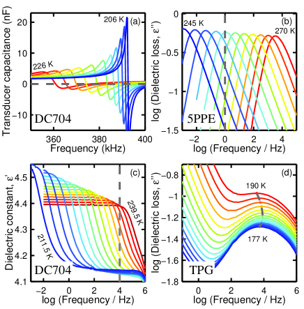
Figure 1: Spectra illustrating the different types of measurements used for probing physical aging. The intersections between the grey dashed lines and the spectra indicate the quantities monitored. (a) Mechanical resonance of a piezo-electric disc; (b) dielectric loss; (c) real part of the dielectric constant at a high frequency, which at the aging temperatures is much above the alpha relaxation frequency; (d) dielectric beta relaxation loss-peak frequency (raw loss-peak frequency with no correction for the alpha process which, however, is insignificant at the aging temperatures).

The three liquids studied are tetramethyl-tetraphenyl-trisiloxane (DC704), 5-polyphenyl-4-ether (5PPE), and tripropylene glycol (TPG). Examples of the measurements behind the aging analysis are given in Fig. 1 (for a more thorough discussion please refer to the Supplemental Material). Figure 2 shows how the monitored quantity $X(t)$ equilibrates upon temperature up and down jumps (black and light blue). There is always a rapid change of $X$. The subsequent aging starts from a short-time plateau, which is most clearly visible for the up-jump data points.

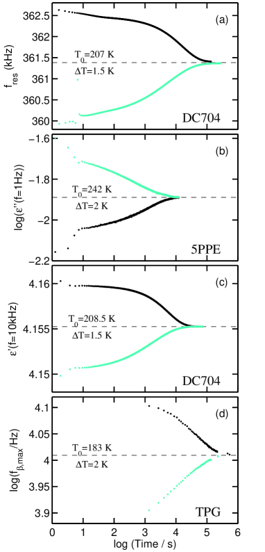
Figure 2: Aging data for temperature jumps for the different quantities probed. Each panel shows a pair of $\Delta T$ up and down jumps to the same temperature $T_{0}$. Up jumps are shown in black and have the characteristic self-accelerated shape, down jumps (in light blue) display self-retarded behavior. (a) Mechanical resonance frequency; (b) logarithm of the dielectric loss at 1 Hz; (c) real part of the dielectric constant at 10 kHz; (d) loss-peak frequency of the dielectric beta relaxation.

Consider a temperature jump initiated at $t=0$, which is studied by monitoring the time development of $X$. The jump starts from equilibrium at temperature $T_{0}+\Delta T$ and ends in equilibrium at $T_{0}$ at which the equilibrium value of $X$ is denoted by $X_{\rm eq}$. Following the convention of the aging literature the time-dependent variation of $X$ after the jump is denoted by $\Delta X(t)\equiv X(t)-X_{\rm eq}$. Thus $\Delta X(t)$ goes from $\Delta X(0)$ to zero as $t\rightarrow\infty$ and equilibrium at $T_{0}$ is attained.

The material time of the TN formalism denoted by $\xi$ is defined from the rate $\gamma(t)$ of the system’s “inner clock” as follows

$$d\xi=\gamma(t)\,dt\,.$$ (1)

The TN formalism implies that for the general temperature variation $T_{0}+\Delta T(t)$ the quantity $\Delta X(t)$ can be written as an instantaneous contribution plus a material-time convolution integral Narayanaswamy (1971),

$$\Delta X(\xi)=C\Delta T(\xi)\,-\,\int_{-\infty}^{\xi}M(\xi-\xi^{\prime})\,\frac{d\Delta T}{d\xi^{\prime}}(\xi^{\prime})\,d\xi^{\prime}\,.$$ (2)

Here $\xi=\xi(t)$ found by integration of Eq. (1). After a jump at $t=0$ from $T_{0}+\Delta T$ to $T_{0}$ it follows from Eq. (2) that $\Delta X(t)=\Delta T(-C+M(\xi))$.

We study jumps small enough that the jump magnitude obeys $\Delta X(0)\propto\Delta T$. In terms of the dimensionless function ${\phi}(\xi)\equiv(dT/dX)(-C+M(\xi))$ one has $\Delta X(t)=\Delta X(0)\,{\phi}(\xi)$ with ${\phi}(0)=1$. Defining the normalized relaxation function $R(t)$ by

$$R(t)\equiv\frac{\Delta X(t)}{\Delta X(0)}\,,$$ (3)

for any temperature jump we thus have

$$R(t)={\phi}(\xi)\,.$$ (4)

We have so far followed Narayanaswamy’s seminal 1971 paper Narayanaswamy (1971) and proceed to convert Eq. (4) into a differential equation. Since $d\xi/dt=\gamma(t)$, the time derivative of $R$ is given by $\dot{R}={\phi}^{\prime}(\xi)\gamma(t)$. Equation (4) implies that $\xi$ is a unique function of $R$; thus ${\phi}^{\prime}(\xi)$ is also a unique function of $R$. Denoting this negative function by $-F(R)$ leads to

$$\dot{R}\,=\,-\,F(R)\,\gamma(t)\,.$$ (5)

Suppose a single parameter $Q$ controls both $X$ and the clock rate. The physical nature of $Q$ is irrelevant Dyre and Olsen (2003); Ellegaard et al. (2007). For small temperature jumps it is reasonable to assume that one can expand $X$ to first order in $Q$: $\Delta X\equiv X-X_{\rm eq}=c_{1}(Q-Q_{\rm eq})$ in which $Q_{\rm eq}$ is the equilibrium value of $Q$ at $T_{0}$ Dyre and Olsen (2003). The clock rate is determined by barriers to be overcome and their activation energies, so one likewise expects a first-order expansion of the form $\ln\gamma-\ln\gamma_{\rm eq}=c_{2}(Q-Q_{\rm eq})$ to apply. Eliminating $Q-Q_{\rm eq}$ leads to $\ln\gamma=\ln\gamma_{\rm eq}+a\Delta X/X_{\rm eq}$ in which $a\equiv c_{2}X_{\rm eq}/c_{1}$ is a dimensionless constant. Introducing the time dependence explicitly via Eq. (3) we have Tool (1946); Petrie (1972)

$$\gamma(t)=\gamma_{\rm eq}\,\exp\left(a\frac{\Delta X(0)}{X_{\rm eq}}R(t)\right)\,.$$ (6)

Substituting this into Eq. (5) leads finally to the basic equation for single-parameter aging following a temperature jump,

$$\dot{R}\,=\,-\,\gamma_{\rm eq}\,F(R)\,\exp\left(a\frac{\Delta X(0)}{X_{\rm eq}}R\right)\,.$$ (7)

The important advance of Narayanaswamy in 1971 was to replace that time’s nonlinear aging differential equations by a linear convolution integral. It may seem surprising that we now propose stepping back to a differential equation Kolvin and Bouchbinder (2012). Consistency with the TN formalism is ensured, however, by the fact that Eq. (7) only applies for temperature jumps. In contrast, the aging differential equations of Tool and others of the form $d(X-X_{\rm eq}(T))/dt=-(X-X_{\rm eq}(T))/\tau(X,T)$ Tool (1946); Ritland (1956) were constructed to describe general temperature histories $T(t)$. Such equations lead to simple exponential relaxation in the linear aging limit ($\Delta T\rightarrow 0$), which is rarely observed, and they cannot account for the crossover effect Scherer (1986).

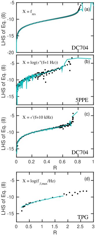
Figure 3: Test of Eq. (8) for the Fig. 2 data by plotting its left-hand side (except for the factor $\gamma_{\rm eq}$) as a function of the normalized relaxation function $R$ (time unit: seconds; the four $a$ parameters were determined from Eq. (11)). For the three first probes the instantaneous change after a temperature jump goes in the same direction as the subsequent aging. The beta loss-peak frequency initially jumps in the opposite direction, which is why $R$ is temporarily larger than unity for this data set (Fig. 4(d)). Data were binned and averaged over ten points, except in (d) where only five points were binned due to scarcity of data. As in Fig. 2 the black dots give the temperature up jumps; the down jumps are marked by a light blue curve connecting the small points.

Equation (7) may be tested without fitting data to analytical functions or knowing $F(R)$. Taking the logarithm of Eq. (7) leads to

$$\ln\left(-\frac{\dot{R}}{\gamma_{\rm eq}}\right)-a\,\frac{\Delta X(0)}{X_{\rm eq}}\,R\,=\,\ln\left(F(R)\right)\,.$$ (8)

For any temperature jump the left-hand side is predicted to be a function of $R$ that is independent of the jump magnitude $\Delta X(0)$. This is tested in Fig. 3 by plotting the left-hand side against $R$ for the data of Fig. 2. The four $a$ parameters have not been optimized for the best fit; they were determined from Eq. (11) derived below.

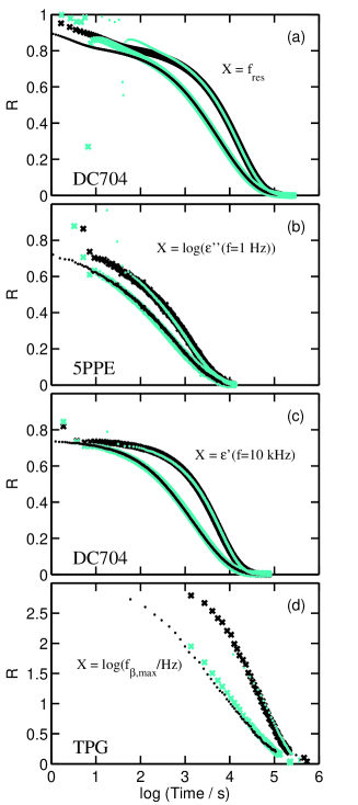
Figure 4: Data (crosses) and predictions based on Eq. (10) (dots) for each of the normalized Fig. 2 data sets. (a) Mechanical resonance frequency; (b) low-frequency dielectric loss; (c) high-frequency dielectric constant; (d) beta loss-peak frequency. Up jumps are in black, down jumps in light blue. Predicted curves are in the same color as the data they are calculated from.

A second test considers two temperature jumps to the same temperature $T_{0}$. The corresponding normalized relaxation functions are denoted by $R_{1}(t_{1})$ and $R_{2}(t_{2})$ with inverse functions $t_{1}(R_{1})$ and $t_{2}(R_{2})$. For times $t_{1}(R_{1})$ and $t_{2}(R_{2})$ corresponding to the same value of the normalized relaxation functions, $R_{1}=R_{2}$, Eq. (7) implies

$$\frac{dR_{1}}{dt_{1}}\,\exp\left(-a\frac{\Delta X_{1}(0)}{X_{\rm eq}}R_{1}\right)\,=\,\frac{dR_{2}}{dt_{2}}\,\exp\left(-a\frac{\Delta X_{2}(0)}{X_{\rm eq}}R_{2}\right)\,.$$ (9)

For time increments $dt_{1}$ and $dt_{2}$ leading to identical changes $dR_{1}=dR_{2}$, if $\Lambda_{12}\equiv a(\Delta X_{1}(0)-\Delta X_{2}(0))/X_{\rm eq}$, Eq. (9) implies $dt_{2}=\exp({\Lambda_{12}R_{1}})dt_{1}$. By integration and identifying $R\equiv R_{1}=R_{2}$ this leads to

$$t_{2}(R)\,=\,\int_{0}^{t_{2}(R)}dt_{2}\,=\,\int_{0}^{t_{1}(R)}e^{\Lambda_{12}R_{1}(t_{1})}\,dt_{1}\,.$$ (10)

This gives a simple recipe for calculating one normalized relaxation function from another. Figure 4 shows the normalized relaxation functions $R(t)$ of the Fig. 2 data (crosses) and those calculated from the other data set via Eq. (10) (dots).

Equation (10) implies $t_{2}(R)-t_{1}(R)=\int_{0}^{t_{1}(R)}(e^{\Lambda_{12}R_{1}(t_{1})}-1)dt_{1}$. A similar expression applies for $t_{1}(R)-t_{2}(R)$. Since $\Lambda_{21}=-\Lambda_{12}$, adding the long-time limits of these expressions leads to the following consistency requirement

$$\int_{0}^{\infty}\big{(}e^{\Lambda_{12}R_{1}(t_{1})}-1\big{)}\,dt_{1}\,+\,\int_{0}^{\infty}\big{(}e^{-\Lambda_{12}R_{2}(t_{2})}-1\big{)}\,dt_{2}\,=0\,.$$ (11)

Since $\Lambda_{12}$ determines $a$, this provides an equation for the $a$ values used in Figs. 3 and 4. The Supplemental Material shows that the $a$ parameters derived in this way are consistent with extrapolations from higher-temperature equilibrium measurements.

In summary, we have presented accurate data for temperature jumps of organic glasses and derived a simplified version of the Narayanswamy’s 1971 aging theory that allows for direct data tests. The new tests do not involve any fitting to analytical functions, as is usually done. In Ref. Hecksher et al., 2010 we also proposed a test of the Narayanaswamy theory not involving such fits, but it was more complicated than the present procedure and did not make predictions for how to calculate all temperare jumps from knowledge of a single one. The test of Ref. Hecksher et al., 2010 involved calculating derivates numerically from data, which is an inherently noisy process. – Crucially, Eq. (7) involves both the normalized and the unnormalized relaxation functions, $R(t)$ and $\Delta X(t)=\Delta X(0)\,R(t)$. This is necessary because a differential equation for only $R(t)$ cannot account for the nonlinearity, whereas a differential equation involving only $\Delta X(t)$ cannot lead to nonexponentiality in the linear limit.

There are other approaches to describing physical aging than the standard TN theory Lunkenheimer et al. (2005); Kolvin and Bouchbinder (2012). The common “single-parameter” assumption of all simple theories is that the quantity monitored correlates to the clock rate $\gamma$. This is also the main ingredient in the approach of Lunkenheimer et al., which assumes a stretched-exponential aging function with a characteristic inverse relaxation time that itself ages according to the same stretched exponential Lunkenheimer et al. (2005); Richert et al. (2013). – In continuing work we are currently investigating the possibility of using higher-order expansions for describing temperature jumps larger than those reported here.