Long-term non-linear predictability of ENSO events over the 20th century

Abstract

We show that the monthly recorded history (1878-2013) of the Southern Oscillation Index (SOI), a descriptor of the El Niño Southern Oscillation (ENSO) phenomenon, can be well described as a dynamic system that supports an average nonlinear predictability well beyond the spring barrier. The predictability is strongly linked to a detailed knowledge of the topology of the attractor obtained by embedding the SOI index in a wavelets base state space. Using the state orbits on the attractor we show that the information contained in the Southern Oscillation Index (SOI) is sufficient to provide average nonlinear predictions for time periods of 2, 3 and 4 years in advance throughout the 20th century with an acceptable error. The simplicity of implementation and ease of use makes it suitable for studying non linear predictability in any area where observations are similar to those that describe the ENSO phenomenon.

1 Introduction

The El Niño Southern Oscillation is a large scale tropical Pacific atmosphere-ocean phenomena. Zebiak1987 , Neelin1998 , Wang2012 one of the stronger quasi-oscillatory pattern observed in the climate system that induces important changes in the global Earth’s gravity field Phillips2012 , influence precise variations of geodetics parameters such as Geocenter Cretaux2002 may play a major role in the generation of seismicity Gillas2010 , or serve as a modulator of the external sun’s influence on Earth’s climate Burn2013 . However teleconnections not only influences climate worldwide but also influences economic, political and social related aspects of the Earth system Bjerknes1969 , Kovats2003 , Brunner2002 , Hsiang2011 . Thus, ENSO signal is a key index representing the complex dynamics of the Earth system as a whole McPhaden2006 . It is therefore understandable that comprehension of its dynamics is one of the most important scientific milestones today and in parallel its prediction is one of the major challenges, and no longer an element solely of interest to climatologists alone.

International efforts to forecast ENSO using both dynamical and statistical methods, have met with some success. Thus, with lead times up to 6 mo, various forecasts performed reasonably well, whereas for longer lead times, that is passing through the boreal spring barrier, the performance becomes rather low, particularly for the most extreme events such as El Niño 1982-83 and 1997-98’s Landsea2000 , Chen2008 . However recent results Ludescher11022014 highlight potential skill in predicting tropical Pacific variability at lead times exceeding 1 year for some events Fedorov . This is an evidence that the ability to predict ENSO events for periods longer than one year and perhaps particularly those leading to greater consequences worldwide is also feasible. However, the previous stage before prediction, is to first show that this goal is achievable. That is, there is at least enough information within the oscillatory system, as represented by the main ENSO index, the Southern Oscillation Index (SOI), that may allow prediction of ENSO events.

The main purpose of this paper is to report that such evidence exists. In a precedent article hfa2010 , a methodology for applying Takens’s embedding theorem Takens1981 to reconstruct an event is developed, by taking into account just the local information contained in a short time series. The physical basis of the method lies in the definition of the local predictability Ding1 . Local predictability limit gives a measure of long time-scale local predictability on the attractor Ding2 . These results outlined the capabilities of the methodology which this local reconstruction method uses to characterize the local and non-linear properties of a given system dynamics. Thus, with the knowledge of the variability over the past 20th century, it was possible to reconstruct local extreme ENSO events (1982-83 and 1997-98), leading by more than two years in advance. Likewise, the method can be applied to arbitrarily large sizes but the search for the relevant embedding state, or - space subspaces that characterize the phenomena requires a high computational cost, hindering the use of the method, and thereby reproduction of results. A simpler but complementary approach allows ease reproducibility, allowing to reconfirm the precedent study. Thanks to a significant breakthrough that overcame the computational and technical difficulties involved in the application of the method to embed a signal of limited temporal extension in a state space. As wavelets2011 it has already been reported that the wavelet space and the embedding space are equivalent in topology, therefore a description is possible by using under Takens’s embedding theorem, which allows to reconstruct a state space which is diffeomorphic to the physical phase space from a time series RevModPhys.65.1331 . Thus, in this analysis, the SOI is considered as a macroscopic variable that has been embedded in the $n$-dimensional state space. So that, we assume that the SOI represents a variable that is a part of non-linear differential equations describing the oscillation. Extending hfa2010 to the problem under consideration, a wavelet decomposition separates the different $n$ state coordinates from the signal equivalently as described in PhysRevLett.45.712 and PhysRevLett.59.845 . Thus liberating us from the tedious searching process for the optimal state spaces as was done previously. Thus, the process’s presented in the precedent investigation can be eased, making it more attractive and straightforward for its application and reproducibility.

Thus, the methodology presented here allows to search whithin the whole length of the times series non linear trajectories that do present the same properties that the non linear trajectories of the attractor of a particular event investigated. Therein it is possible using the sole non-linear information already present whitin a time series to find similar attractor-trajectories that allows to investigate if a particular ENSO event is reproducible to a certain extent.

2 Methodology

To achieve this goal we first define an n-dimensional state space $\mathbf{E_{n}}$. The evolution of the system in this state space is recorded in a state trajectory given by $\mathbf{r}_{n}(t)=(S_{1}(t),...,S_{n}(t))$, where quantities $S_{1}(t),...,S_{n}(t)$ are obtained by wavelet decomposition of the SOI signal Konnen1998 . From the original signal, a given number $n$ of component signals $S_{i}$ are obtained by means of wavelet filtering the monthly SOI index between the years 1866-2013. We decompose the SOI data using a Discrete Wavelet Transformation (DWT) multiresolution algorithm with a Morlet mother wavelet function Craigmile2002 , Murguia2011 . In our case we choose an 8 level decomposition, considering the monthly time series resolution. Because fewer levels did not allow to separate efficiently the interannual time scales or capture interdecadal time scales efficiently that characterize ENSO Wang2012 , so each of the components ($S_{i}$, $i$ from 1 to 8) represent a given bandwidth (1-2 intra-seasonal, 3-5 interannual, 6-8, decadal to interdecadal) whereas the last component $S_{9}$ represents lowest frequencies, that describes the trend. In other words $SOI=S_{1}+...+S_{9}$. In this paper we use a state space $\mathbf{E_{9}}$ following Tsonis2009 encrypting all information contained in the SOI in the state trajectory, but we also define a six dimensional subspace, $\mathbf{E_{6}}$ where the state trajectory is given by $\mathbf{r_{6}}(t)=(S_{4}(t),...,S_{9}(t))$ containing information only in the low frequency range (lower than $1/yr)$. We compute the low frequency part of the SOI signal as $S_{L}=S_{4}+...+S_{9}$.

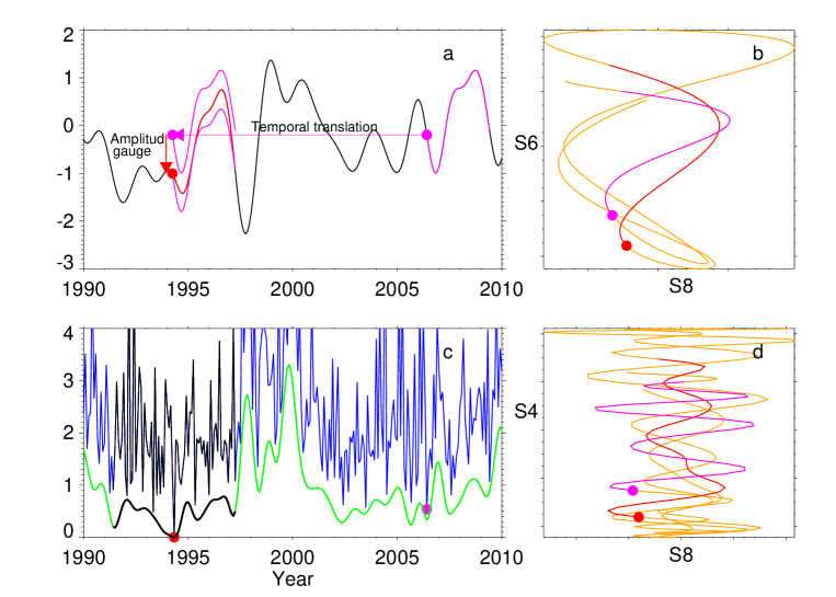
Figure 1: Figure details the steps to be carried out to determine which part of the signal $S_{L}$ that is most similar to the event to be predicted. In panel a the $S_{L}$ signal is plotted. The red dot is the starting point of the event that corresponds to the first starting state point in Figure 2, while the red section indicates the extent of the event to be predicted. The magenta point indicates the point corresponding to the nearest point on the chosen orbit. In panel c the blue line is the Euclidean distance between the starting point and each point of the state trajectory calculated in $\mathbf{E_{9}}$, while the green curve is the Euclidean distance between the starting point and each point of the path that was calculated in $\mathbf{E_{6}}$. In panels b and d we plot $(S_{8},S_{6})$ and $(S_{8},S_{4})$ two-dimensional projections of the attractor, respectively. The orange curves are projections of the state trajectory.

The event (An El Niño or La Niña event) to be predicted $S_{L_{i}}$ is selected from $S_{L}$ (represented by the red segment in Figure 1a). The first point in $S_{L_{i}}$ (represented by a red dot in Figure 1a) is the starting point at time $t_{sp}$ and the terminal point is located by $T$ steps in the future. To select another part of the signal $S_{L}$ that enables to reproduce the relevant features of the $S_{L_{i}}$ event, we seek a state point of the state trajectory in the attractor around which the embedded signal $SOI$ has the same topological features like than around the starting point of the event. Thus, both state points are located about the same region in the attractor. Figure 1b and Figure 1d shows bidimensional projections of the state trajectory (in orange) around the attractor, while red and magenta colors plots shows the selected event and the most similar event, respectively. To accomplish this task we calculate the Euclidean distance of all state points in the state trajectory to the starting state point. In the $\mathbf{E_{9}}$ reconstructed state space the Euclidean distance between each state point of state trajectory to the starting state point is given by $d(t)=\parallel\mathbf{r_{9}}(t)-\mathbf{r_{9}}(t_{sp})\parallel$, which is plotted in blue in Figure 1c. Then, we collect the times, $t_{j}$, where the curve $d=d(t)$ exhibits local minima. Each selected local minimum of the function $d(t)$ corresponds to a state point on each orbit that is closest to the starting state point in the reconstructed state space $\mathbf{E_{9}}$. This search is performed away from a region of $T$ steps from each side (to the past and the future) of the starting point, $t_{sp}$ (regions in black in Figure 1c). For each of the collected times, $t_{j}$ a piece of the corresponding $S_{L}$ of $T$ steps long is extracted into its own future (that is $S_{L_{j}}$). As shown in Figure 1a, the $S_{L_{j}}$ piece (magenta) is then moved to the starting point, $t_{sp}$ (the red dot) through a temporal translation (the magenta arrow). In addition, the translated signal (the $S_{L_{j}}$ piece), as an amplitud gauge (the red arrow in Figure 1), is shifted up or down so that its first point (originally at $t_{j}$) matches the value of $S_{L}$ at the starting point at time $t_{sp}$ (the event to be predicted, that is $S_{L_{i}}$). In addition, the physical consistency implies that all the selected $S_{L_{j}}$ pieces must contain the same number of maxima and minima than the chosen event in $S_{L}$ ($S_{L_{i}}$). Finally, of all the $S_{L_{j}}$ pieces selected and translated as described, the piece that contains the same number of maxima and the same number of minima as $S_{L_{i}}$ which produces the least quadratic difference is definitely chosen (the magenta dot in Figure 1).

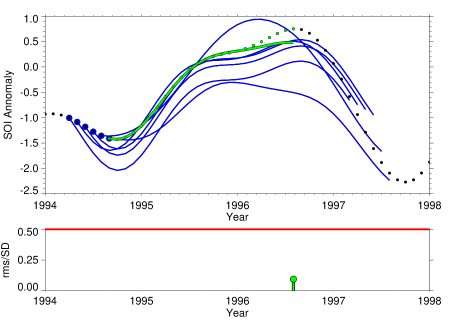
Figure 2: Above: The Figure outlines the steps followed in the procedure for obtaining an average prediction for two years. Points in black are the monthly amplitudes of low-frequency SOI index ($S_{L}$). The blue points are the starting points for each prediction for three years, which are drawn with blue lines.The green curve is the two years average nonlinear prediction. Below: The red line marks the boundary where the mean square error of the average nonlinear prediction is half the standard deviation of $S_{L}$. The green bar at the bottom indicates the mean square error relative to the standard deviation of $S_{L}$ of the average nonlinear prediction drawn in green.

To make a robust estimate of the event we perform an average of six consecutive months of predictions resulting a $T_{eff}=T-12$ months prediction, which is plotted in green in Figure 2, after a necessary second amplitude gauge. Thus, the averaged prediction begins on the date of the last prediction used for constructing the 6 monthly mean that has the final date of the first prediction used. Thus on average an initial three years local prediction reduces to an mean prediction of about two years.

Finally we compute the error of the prediction of these two year long prediction by normalizing to the standard deviation of $S_{L}$. The error is reported as a bar below the signal. The red line in Figures 2 to 5 indicate the threshold of $0.5$ which means that the error of the prediction reach the half of the standard deviation ($SD$) of the whole signal $S_{L}$.

3 Results

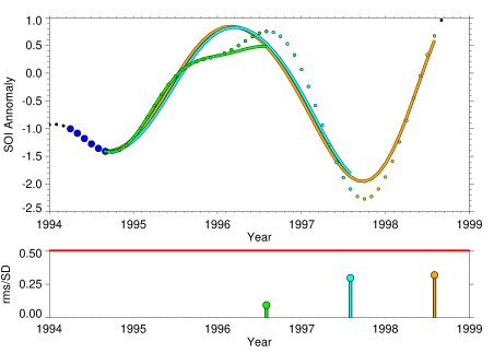
Figure 3: Above: Average non-linear predictions for two years lead (in green) and the $S_{L}$ time series (in black) are drawn. Below: The relative error. The red line indicates the $0.5$ threshold. The green, cyan, and orange bars are the average non linear predictions error for $T_{eff}=2,3$ and $4$ years, respectively.

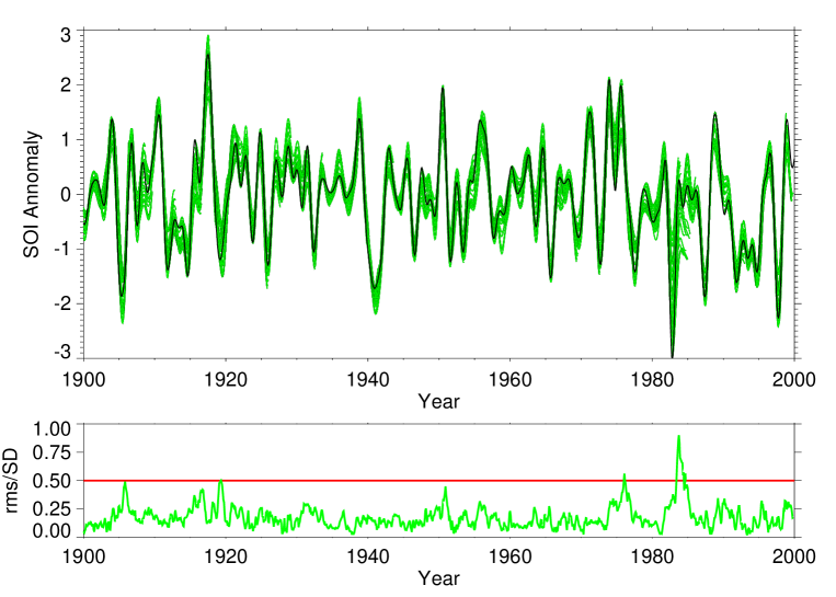
Figure 4: Above: The performance of the procedure for average non-linear predictions with $T_{eff}=2$ years of El Niño during the 20th century. Below: The relative error. The red line indicates the $0.5$ threshold.

Remarkably (Figures 2, 3 and 4) one of the most extreme event of the 20th century, namely the 1997-98 Niño event could be clearly anticipated well beyond a two year lead to the least. Thus it is possible to find trajectories in the SOI time series that present the same nonlinear characteristics than the variability of the 1997-98 event. Thus, the relative error for the two year lead Figure 4b is below the 0.5 threshold. Instead for the 1982-83 event, the relative error is well above the 0.5 threshold. That is, meaning that it is not possible to find any correct trajectory/attractor within the whole 1878-2013 time span that present the same non-linear properties than the 1982-83 event.

The analysis of relative error histograms (Figure 5a) shows that when the lead times increases (from 2 to 4 years), the averaged relative error indeed increases, from $0.177$, $0.298$ and $0.389$ for $T_{eff}=2,3,4$ years respectively (see Figure 5a and Table 1).

Indeed while increasing the lead times, the error for the particular 1982-83 and 1997-98 events increases. However, for the El Niño 1997-98, while increasing the lead times, the relative error always falls below the 0.5 threshold (lesser than 0.37). The orbit/trajectories that are closer to an event and that allows the accurate averaged prediction, changes depending on lead time (and can change from one month to another). However, the analysis of Figure 5b shows that the histogram of closer trajectories is a Gaussian-shaped distribution, that is, in general the non-linear prediction always finds a trajectory in the vicinity of the event in the state space.

Thus, if we had to look for the trajectories used for the construction of the 2 year lead prediction of the particular 1997-98 event, throughout the span of the event, these would be those of the 1911, 1972-73 and 1982-83 events. Interestingly the orbits/trajectories that naturally emerges for the 1982-83 event, and eventhough this event rises above the 0.5 threshold, are indeed preferentially the 1997-98 (in the future) and also the 1901-02 events.

4 Discussion and Conclusions

As already stated the physical support of this methodology consider the dynamics of ENSO described as a dynamic system. Thus, the signal, can be considered as a solution for a nonlinear system of differential equations describing the oscillation. In virtue of the Takens’s theorem the signal is embedded in the $9$-dimensional state space $\mathbf{E_{9}}$ so that the relevant information contained in the system is encrypted in a state trajectory of the system. With this procedure the state points of the state trajectory, ie, the states of the system are arranged in orbits around an attractor. The idea behind this methodology relies on possibility to find in past or future evolutions of a time series events that present the same characteristics (orbits around the attractor) than the event investigated. The closest orbits increases the capacity of event predictability.

Once an event $S_{L_{i}}$ is selected in the signal $S_{L}$, the starting point at time $t_{sp}$ and a time interval of prediction $T$ is determined. The starting point of the selected event corresponds to a system state point on the attractor. To find an event in the signal, $S_{L_{j}}$, corresponding to a similar solution of the same set of deferential equations, we determine the set of state points $t_{sp_{j}}$ that are in a region around the starting state point in the attractor (in $\mathbf{E_{9}}$). We remark that the reconstructed state space $\mathbf{E_{9}}$ is diffeomorphic to the physical phase space RevModPhys.65.1331 .

The selection of the most similar piece of the event signal is by performing the choicest among all segments of length $T$, starting at state points that are in vicinity of the starting state point of the event. These datas provide the least deviation standard with the same number of peaks and the same number of minima as the event signal.

The most important result of this study is that the so-called SOI anomaly corresponds to the dynamics of a nolinear oscillator having complex regularities and exhibits an acceptable level of accuracy of average non-linear predictability in the range between 2 and 4 years of time span. Although the topology of the attractor is unknown, for each event it is always possible to find an orbit corresponding to another event that ocurs in the past or in the future of the starting point which has the same category. The knowledge of the topological structure of the attractor is a necessary task for forecasting. In our method, as discussed previously, we chose the best orbit in the attractor. The histograms at the bottom of Figures 5a and 5b shows that there is no deterministic rule that allows us to choose the right orbit with certainty, although a clear trend towards the nearest orbit was observed.

Note that indeed the methodology here used, as it uses a wavelet filter bank with different scales does take in account, when constructing the orbit attractor for a particular event, a part of the closest (past or future) evolution of the time series. However, this is performed only for constructing the attractor and search for similitudes within the whole length of the time series and not for constructing the prediction. Therefore, this lapse is already existing and is not built in any way with the method. In addition, the methodology find trajectories that are far away in time from the event analysed. Also, in a precedent paper hfa2010 we already demonstrated that the methodology worked although search for relevant embedding space was tedious and with high computer cost. Here we only extend the methodology, thanks to the wavelet space to a set of embedding state spaces that indeed facilitates the search for closest orbits and therefore for similar trajectories within the length of the time series. In other words the wavelet filtering bank does not interfere with the time selected. Finally the method is not filter dependent. Thus, we tested the methodology with two different filtering banks, that is with Empirical modal decomposition EMD Huang2005 and Singular Spectrum analysis SSA Golyandina2013 . In both cases, and particularly for SSA, the methodology could reconstruct correctly most events throughout the 20th century but failed for the 1982/83 event.

Although we do not know exactly the selection rule to determine the optimal orbits that allows forecasting that does not invalidate the fact that the SOI signal has built enough information to reproduce events over at least a 2 years span, surpassing throughout the 20th century, with an acceptable error, with exception of the 1982-1983 event.

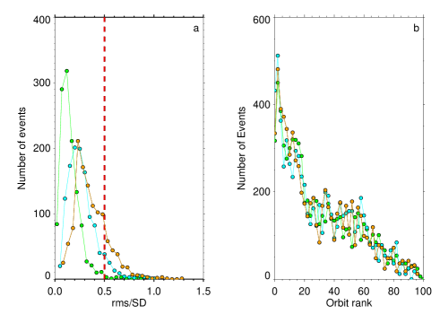
Figure 5: a) Histograms of the relative errors of the average non-linear predictions of El Niño during the 20th century are shown. Relative errors for 2, 3 and 4 years are depicted in green, cyan and orange colors, respectively. b) the histograms of the rank of the selected orbit for each non-linear prediction is been represented. The histogram of orbit rank for 2, 3 and 4 years are represented using green, cyan and orange colors, respectively.

Table 1: Mean, Variance, Skweness and Kurtosis of normalized errors distributions shown in Figures 5a and 5b.

$T_{eff}$	$E_{n}$	M	V	S	K
2	$E_{9}$	0.177	0.011	2.145	8.056
3	$E_{9}$	0.298	0.020	1.404	3.090
4	$E_{9}$	0.389	0.028	1.147	2.067
2	$E_{6}$	0.235	0.019	1.825	4.927
3	$E_{6}$	0.379	0.035	1.236	2.338
4	$E_{6}$	0.483	0.069	4.080	29.49

- (1) Zebiak, S.E. and M.A. Cane (1987) A model El Nino Southern Oscillation. Mon. Wea. Rev. 115:2262–2278.
- (2) Neelin, J. D., D. S. Battisti, A. C. Hirst, F.-F. Jin, Y. Wakata, T. Yamagata, and S. E. Zebiak (1998) ENSO theory, J. Geophys. Res. 103(C7):14261–14290.
- (3) Wang, C. and Deser, C. and Yu, J.-Y. and DiNezio, P. and Clement, A. (2012) El Niño and Southern Oscillation (ENSO): A Review. Coral Reefs of the Eastern Pacific 3–19.
- (4) Phillips, T., R. S. Nerem, B. Fox-Kemper, J. S. and Famiglietti, J. S. and B. Rajagopalan V(2012) The influence of ENSO on global terrestrial water storage using GRACE, Geophys. Res. Lett. 39:L16705.
- (5) Cretaux, J.-F., L. Soudarin, F. J. M. Davidson, M.-C. Gennero, M. Bergé-Nguyen, and A. Cazenave (2002) Seasonal and interannual geocenter motion from SLR and DORIS measurements: Comparison with surface loading data, J. Geophys. Res. 107(B12):2374.
- (6) Guillas S., Day S. J., McGuire B. (2010) Statistical analysis of the El Niño Southern Oscillation and sea or seismicity in the eastern tropical Pacific, Philosophical Transactions of the Royal Society A 368:2481–2500
- (7) Burn, M. J. and Palmer, S. E. (2014) Solar forcing of Caribbean drought events during the last millennium. J. Quaternary Sci. 29(8): 827–836.
- (8) Bjerknes, J. (1969)., Atmospheric teleconnections from the equatorial Pacific, Mon. Weather, Rev. 97:163–172.
- (9) Kovats R, Bouma M, Hajat S, Worrall E, Haines A (2003) El Niño and health. Lancet 362(9394):1481–-1489.
- (10) Brunner A. (2002) El Nino and World Primary Commodity Prices: Warm Water or Hot Air?, Review of Economics and Statistics, 84(1):176–183.
- (11) Hsiang, S. M., K. C. Meng, and M. A. Cane (2011) Civil conflicts are associated with the global climate. Nature 476(7361):438–-441.
- (12) McPhaden, M. J., S. E. Zebiak, and M. H. Glantz (2006) ENSO as an Integrating Concept in Earth Science, Science, 314(5806):1740–1745.
- (13) Christopher W. Landsea and John A. Knaff (2000) How much skill was there in forecasting the very strong 1997–98 el niño?. Bull. Amer. Meteor. Soc. 81: 2107–2119.
- (14) Chen, D., M. A. Cane (2008) El Niño prediction and predictability Original Research Article. J. Comput. Phys. 227(7):3625–3640.
- (15) Ludescher, Josef and Gozolchiani, Avi and Bogachev, Mikhail I. and Bunde, Armin and Havlin, Shlomo and Schellnhuber, Hans Joachim (2014) Very early warning of next El Niño. Proceedings of the National Academy of Sciences 111:2064–2066.
- (16) Fedorov, A.V. and S.L. Harper and S.G. Philander and B. Winter and A. Wittenberg (2003) How Predictable is El Niño?, Bull. Amer. Meteor. Soc. 64:911–919.
- (17) Astudillo, H. F. and Borotto, F. A. and Abarca-del-Rio, R. (2010) Embedding reconstruction methodology for short time series - application to large El Niño events, Nonlinear Processes in Geophysics 17:753–764.
- (18) F. Takens (1981) Lecture Notes in Mathematics. Springer Berlin 898:366–381.
- (19) Ruiqiang Ding and Jianping Li, Nonlinear finite-time Lyapunov exponent and predictability Physics Letters A, 364, 5 (2007), pp. 396–400.
- (20) Ruiqiang Ding and Jianping Li (2008) Nonlinear local Lyapunov exponent and the quantification of local predictability, Chinese Physics Letters, 25(5):1919–1922.
- (21) You Rong-Yi and Huang Xiao-Jing (2011) Phase space reconstruction of chaotic dynamical system based on wavelet decomposition Chinese Physics B, 20(2):02055.
- (22) Abarbanel, Henry D. I. and Brown, Reggie and Sidorowich, John J. and Tsimring, Lev Sh. (1993) The analysis of observed chaotic data in physical systems. Rev. Mod. Phys. 65(4):1331-1392.
- (23) Packard, N. H. and Crutchfield, J. P. and Farmer, J. D. and Shaw, R. S. (1980) Geometry from a Time Series Phys. Rev. Lett., 45(9):712–716.
- (24) Farmer, J. Doyne and Sidorowich, John J. (1987) Predicting chaotic time series, Phys. Rev. Lett., 59(8):845–848.
- (25) Koennen, G. P. and Jones, P. D.and Kaltofen, M. H. and Allan, R. J. (1998) Pre -1866 extension of the Southern Oscillation Index using early Indonesian and Tahitian meteorological readings J. Climate 11: 2325–2339.
- (26) Tsonis, A. (2009) Dynamical changes in the ENSO system in the last 11,000 years Climate Dynamics, 33: 1069–1074
- (27) Craigmile, P.F., and Percival, D.B. (2002) Wavelet-based trend detection and estimation. In: Encyclopedia of Environmetrics, A. El-Shaarawi and W. W. Piegorsch (Ed): John Wiley & Sons. ISBN 9780471899976
- (28) Murguía, José S. and Haret C. Rosu (2011) Discrete Wavelet Analyses for Time Series. In: Discrete Wavelet Transforms-Theory and Applications, Dr. Juuso T. Olkkonen (Ed.): InTech, ISBN: 978-953-307-185-5.
- (29) Golyandina, N., and A. Zhigljavsky (2013) Singular Spectrum Analysis for time series. Springer Briefs in Statistics, Springer, ISBN 978-3-642-34912-6., 120 pages
- (30) Huang, N. E.; Shen, S. S. P. (2005). Hilbert-Huang Transform and its Applications. London: World Scientific. ISBN 978-9812563767.