Control-based continuation: bifurcation and stability analysis for physical experiments

Abstract

Control-based continuation is technique for tracking the solutions and bifurcations of nonlinear experiments. The basic idea is to apply the method of numerical continuation to a feedback-controlled physical experiment. Since in an experiment it is not (generally) possible to set the state of the system directly, the control target is used as a proxy for the state. The challenge then becomes to determine a control target such that the control is non-invasive, that is, it stabilises a steady-state (or periodic orbit) of the original open-loop experiment without altering it otherwise.

Once implemented, control-based continuation enables the systematic investigation of the bifurcation structure of a physical system, much like if it was numerical model. However, stability information (and hence bifurcation detection and classification) is not readily available due to the presence of stabilising feedback control. This paper uses methods from the system identification community to extract stability information in the form of Floquet multipliers from the closed-loop experiment, thus enabling the direct detection of bifurcations. In particular, it is shown that a periodic auto-regressive model with exogenous inputs (ARX) can be constructed that approximates the time-varying linearisation of the experiment around a particular periodic orbit. This method is demonstrated using a physical nonlinear tuned mass damper.

1 Introduction

Control-based continuation is a systematic method for performing bifurcation studies on physical experiments. Based on modern feedback control schemes it enables dynamical phenomena to be detected and tracked as system parameters are varied in a similar manner to how nonlinear numerical models can be investigated using numerical continuation. Control-based continuation was originally developed as an extension to Pyragas’ time-delayed feedback control [1, 2, 3] to make it more robust and suitable for parameter studies [4], though its current implementation contains no elements of time-delayed feedback.

The use of feedback control for the investigation of nonlinear systems is not new; in addition to time-delayed feedback, methods such as OGY control [5] have previously been employed to provide non-invasive control to stabilise unstable orbits and investigate dynamical phenomena. Indeed, previous authors have gone as far as to implement such control schemes within parameter continuation studies to numerically simulate particular experiments such as atomic force microscopes [6] or reaction kinetics [7]. Control-based continuation goes beyond these particular methods to allow the use of almost any feedback control scheme and, as such, it is a general purpose tool applicable to a wide range of physical experiments.

Control-based continuation has been successfully applied to a range of experiments including a parametrically excited pendulum [8], nonlinear energy harvesters [9, 10] and a bilinear oscillator [11, 12]. In each case, periodic orbits have been tracked through instabilities such as saddle-node bifurcations (folds) thus revealing a great deal of dynamical information about the system in question, including the location of a codimension-2 cusp bifurcation in one case [13]. As well as bifurcations, other dynamic features such as backbone curves can also be tracked with control-based continuation [14].

Although the basic scheme for control-based continuation is well established (an overview is provided in Sec. 2), it lacks many of the features of standard numerical continuation schemes such as bifurcation detection. Only saddle-node bifurcations (folds) can be detected readily and that is because they are geometric features in the solution surface. Bifurcations such as period-doubling bifurcations are not geometric features and can go undetected due to the stabilising affect of the feedback controller. Similarly, the inclusion of the feedback controller means that methods for calculating eigenvalues/Floquet multipliers and basins of attraction from experiments such as [15, 16, 17] are not helpful since they indicate the stability of the closed-loop system rather than the open-loop system.

In this paper we consider only periodically forced systems and hence study periodic orbits, though there is no reason that the methods developed should not be applicable to autonomous systems as well. In Sec. 3, we propose a method for calculating the stability (the Floquet multipliers and associated stable and unstable eigendirections) based on the estimation of a local linearisation around a stabilised periodic orbit. We demonstrate the effectiveness of this method in Sec. 4 and Sec. 5 by applying it to a (physical) nonlinear mass-spring-damper system where the nonlinearity is geometric in nature — the springs are mounted perpendicular to the direction of motion.

2 Control-based continuation

Numerical continuation is a path following method used to track solution branches as parameters of the system in question are varied. In a nonlinear system, these solution branches can encounter bifurcations at particular parameter values which results in a qualitative change in the dynamics of the system. Numerical continuation enables these bifurcations to be detected and tracked in turn. It is typically applied to differential equation models but it can be used more widely, for example on finite element models.

At a basic level, numerical continuation tracks the solutions of an arbitrary nonlinear function, a zero problem given by

$$f(x,\lambda)=0,\qquad f:\mathbb{R}^{n}\times\mathbb{R}^{p}\rightarrow\mathbb{R}^{m}$$ (1)

where $x$ is the system state and $\lambda$ is the system parameter(s). A common example of this is tracking the equilibria of an ordinary differential equation with respect to a single parameter. In this case $n=m$ and $p=1$ in Eq. (1), that is, $f=0$ defines a one-dimensional curve. Alternatively the function $f$ can arise from the discretisation of a periodic orbit. Numerical continuation works in a predictor-corrector fashion; at each step a new solution $\tilde{x}$ is predicted from previously determined solutions and then the solution is corrected using a nonlinear root finder applied to the function $f$ (typically a Newton iteration). The use of a nonlinear root finder means that the stability or instability of solutions is unimportant. In certain circumstances (for example, near a fold or saddle-node bifurcation) the function $f$ must be augmented with an additional equation — the pseudo-arclength equation — which enables the numerical continuation scheme to track solution curves that double back on themselves. In these circumstances, without the pseudo-arclength equation the correction step for a fixed set of parameter values $\lambda$ will fail since no solution exists. For extensive information and guidance on numerical continuation see the textbooks [18, 19]. Numerical software is also readily available in the form of CoCo [20] and AUTO [21] amongst others.

Control-based continuation is a means for defining a zero-problem based on the outputs of a physical experiment, thus enabling numerical continuation to be applied directly without the need for a mathematical model. To do this there are two key challenges to overcome. 1) In general, it is not possible to set the state $x$ of the physical system and so it is not possible to evaluate $f$ at arbitrary points. 2) The physical system must remain around a stable operating point while the experiment is running. While a numerical model going unstable might prove to be a mild annoyance, a physical system going unstable can prove dangerous.

In order to overcome these challenges, a feedback controller is used to stabilise the system and the control target (or reference signal) acts as a proxy for the system state. The feedback controller takes the form

$$u(t)=g(x^{*}(t)-x(t))$$ (2)

where $x^{*}(t)$ is the control target and $g$ is a suitable control law such as proportional-derivative (PD) control (as used in this paper) where

$$u(t)=K_{p}(x^{*}(t)-x(t))+K_{d}(\dot{x}^{*}(t)-\dot{x}(t)).$$ (3)

For the method outlined in this paper, the choice of control law is at the discretion of the user; any suitable stabilising feedback control scheme can be used. The challenge here is to devise a scheme for embedding the feedback control within the numerical continuation such that the controller becomes non-invasive, that is, the controller does not affect the locations of any invariant sets in the experiment such as equilibria or period orbits. This requirement for non-invasiveness defines the zero problem; a control target must be chosen such that the control action

$$u(t)\equiv 0.$$ (4)

In this paper, we consider the case of a periodically forced experiment with forcing frequency $\omega$ and, as such, only consider periodic motions. In this case it is appropriate to consider a Fourier discretisation of Eq. (4) and so find the coefficients of the Fourier series of the control target $x^{*}(t)=A^{x^{*}}_{0}/2+\sum_{j=1}^{m}A^{x^{*}}_{j}\cos(j\omega t)+B^{x^{*}}_{j}\sin(j\omega t)$ such that Eq. (4) is satisfied. (In other circumstances different discretisations may be appropriate.) In this case the control action $u$ has a Fourier series representation given by

$$u(t)=\frac{A^{u}_{0}}{2}+\sum_{j=1}^{m}A^{u}_{j}\cos(j\omega t)+B^{u}_{j}\sin(j\omega t).$$ (5)

where the Fourier coefficients $A^{u}_{j}$ and $B^{u}_{j}$ are derived directly from the measured control action Eq. (2), that is,

$$A^{u}_{j}=\frac{\omega}{\pi}\int_{0}^{\frac{2\pi}{\omega}}g(x^{*}(t)-x(t))\cos(j\omega t)\operatorname{d}t,\quad\text{for}\ j=0,1,2,\ldots$$ (6a)

$$B^{u}_{j}=\frac{\omega}{\pi}\int_{0}^{\frac{2\pi}{\omega}}g(x^{*}(t)-x(t))\sin(j\omega t)\operatorname{d}t,\quad\text{for}\ j=1,2,\ldots.$$ (6b)

Hence the discretised zero problem is defined as

$$0=A^{u}_{j},\quad 0=B^{u}_{j}\quad\forall j.$$ (7)

To solve Eq. (7) standard root finding algorithms can be used, however, any required derivatives must be estimated using finite differences from experimental data after adjusting the experiment inputs. Consequently, gradient-based methods can be slow despite their good convergence rates. In previous publications a Newton-Broyden method, which avoids recomputing derivative information for successive iterates, has proven effective [8, 10, 11].

In this paper, since the control acts through the same mechanism as the forcing, we are able to use a quicker method which exploits the fact that we are performing a parameter study in the forcing amplitude [13]. Consider the case where the total input to the system is given by

$$i(t)=p(t)+u(t)$$ (8)

where $p(t)$ is the forcing signal and $u(t)$ is the control action. Furthermore, we consider the case of sinusoidal forcing where

$$p(t)=a\cos(\omega t)+b\sin(\omega t).$$ (9)

For an arbitrary control target $u^{*}(t)$ and forcing input $p(t)$, the Fourier coefficients of Eq. (5) will be non-zero. However, the contribution in the fundamental mode (coefficients $A^{u}_{1}$ and $B^{u}_{1}$) can be lumped together with the coefficients $a$ and $b$ of the forcing term giving a new effective forcing amplitude of

$$\Gamma=\sqrt{\left(a+A^{u}_{1}\right)^{2}+\left(b+B^{u}_{1}\right)^{2}}.$$ (10)

Hence, once the higher Fourier modes of the control action $u(t)$ are set to zero (as described below), the total input to the system will be $i(t)=\Gamma\cos(\omega t+\phi)$ (the phase $\phi$ is unimportant since the system is time invariant). In essence, instead of setting the forcing amplitude and trying to calculate the correct corresponding control target, we set the control target and measure the corresponding forcing amplitude.

Though this procedure leaves the $A^{u}_{0}$ and the higher harmonics untouched, the corresponding control target coefficients required to set the control action to zero can be quickly determined using a fixed-point iteration. In an iterative manner the remaining coefficients of the control target $x^{*}(t)$ are simply set equal to the measured coefficients of the system response $x(t)$, the iteration finishes when the response and the control target remain equal for a certain period of time. For the system described below, this takes a single iteration.

A fixed-point iteration cannot be applied to the coefficients of the fundamental mode since, generically, instabilities in the system will manifest in the fundamental mode.

It is important to emphasise that this procedure does not depend on the specifics of the control law used in the experiment. All that is required is that smooth changes in the control target $x^{*}(t)$ result in smooth changes in the Fourier coefficients Eq. (6). As such, this method is convenient in realistic settings where the control law is more sophisticated than simple PD control and filtering of the signal is required; these effects are simply captured in the control action $u(t)$ and fed into Eq. (6).

3 Identification of a linearisation

For a typical ordinary differential equation model, the right-hand side of which is given by $h(x(t))$, the Floquet multipliers and hence stability of a periodic orbit are determined by integrating over one period the first variational equation

$$\frac{\operatorname{d}y}{\operatorname{d}t}=A(\hat{x}(t))y(t)$$ (11)

where $y(t)$ represents the deviation from a predetermined periodic orbit $\hat{x}(t)$ and the Jacobian matrix $A$ is calculated from the derivatives of $h$ with respect to $x$ evaluated along the periodic orbit given by $\hat{x}(t)$ (as such $A$ is a time varying quantity).

In the context of control-based continuation, even determining whether an orbit is stable or unstable is problematic due to the presence of stabilising feedback control. In [12] a number of measures are suggested to overcome this problem but all require turning off the feedback control for a period of time; in many situations this is not desirable as damage could be caused to the experiment or even the experimenter. As such, here we attempt to fit a time-varying linearisation using techniques from the system identification community. From the fitted time-varying linearisation we are able to calculate the corresponding Floquet multipliers and hence the stability properties of the periodic orbit.

We start by assuming that the experiment of interest is undergoing a periodic motion $\hat{x}(t)$ for a given forcing input $\hat{i}(t)=\hat{p}(t)+\hat{u}(t)$ (cf. Eq. (8)). In order to generate data with which to fit a time-varying linearisation, the system is perturbed using filtered Gaussian white noise $\eta(t)$ such that the total input to the experiment is

$$i(t)=\hat{i}(t)+\eta(t)+u(t)-\hat{u}(t).$$ (12)

The additional $u(t)-\hat{u}(t)$ term arises due to the presence of the feedback controller acting against the applied perturbation. (Details of $\eta(t)$ are below.) Finally, we define the perturbed system response

$$y(t)=x(t)-\hat{x}(t)$$ (13)

and, similarly, the perturbed system input

$$k(t)=i(t)-\hat{i}(t).$$ (14)

Rather than try to fit a continuous time model of the response to perturbations such as Eq. (11), which requires the estimation of derivatives from experimental data, we instead fit the coefficients of a discrete-time multiple-input multiple-output (MIMO) auto-regressive model with exogenous inputs (ARX) of the form

$$B(q^{-1})\mathbf{y}(T)=A(q^{-1})\mathbf{k}(T)+\mathbf{e}(T)$$ (15)

where $\mathbf{y}(T)=[y(T-i/m)]_{i=0\ldots m-1}$, $\mathbf{k}(T)=[k(T-i/m)]_{i=0\ldots m-1}$ and $\mathbf{e}(T)=[e(T-i/m)]_{i=0\ldots m-1}$ are vectors of data points of the perturbed system response, the perturbed system input (due to the control action and an additional random perturbation) and the model error respectively, sampled across a single period of oscillation and $q^{-1}$ is the backward shift operator [22, Sec. 6.2]. Thus $\mathbf{y}(T)$ corresponds to a discretisation of the perturbed system response using $m$ points over the period; this discretisation is illustrated in Fig. 1. $B(q^{-1})$ and $A(q^{-1})$ are square $m\times m$ matrices of polynomials in $q^{-1}$; here we restrict the polynomials to being first order (at most). Thus Eq. (15) acts as a period map with all the dynamics of interest encoded in $B(q^{-1})$. (The matrix $A(q^{-1})$ though required for system identification are not used to infer stability.)

The model error $\mathbf{e}(T)$ is not measured directly but is minimised by the particular system identification method used on Eq. (15).

ARX models are used extensively in the system identification and time series analysis communities. Their simplicity has seen them applied to a wide range of topics. They are particularly appropriate in situations where discretely sampled data is available as they avoid the need of estimating derivatives. For more information see the textbook by Hamilton [23] or one of the many other books on this topic.

Figure 1: An example discretisation of the perturbed response of a periodic orbit with $m=5$ and $n=2$; the period of the orbit is normalised to $1$. Here $\mathbf{y}=[y_{0},y_{1},y_{2},y_{3},y_{4}]$. Since $n=2$, $y_{0}$ is purely a function of $[y_{1},y_{2}]$ and $[k_{0},k_{1},k_{2}]$. Similarly, $y_{4}$ is purely a function of $[y_{0}q^{-1},y_{1}q^{-1}]$ and $[k_{4},k_{0}q^{-1},k_{1}q^{-1}]$, where $q^{-1}$ is the backward shift operator. Thus the linearised model Eq. (15) allows the construction of a linear period map from $\mathbf{y}q^{-1}$ to $\mathbf{y}$.

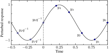
At each point we assume linear observability to state that the next point in the time evolution of the linearisation is determined entirely by the previous $n$ points alone. We assume that $n<m$ (increase the value of $m$ as appropriate) to obtain a banded matrix structure for $B(q^{-1})$ of

$$B(q^{-1})=\begin{bmatrix}1&b_{1,1}&\cdots&b_{1,n-1}&b_{1,n}&0&0&\cdots&0\\ 0&1&\cdots&b_{2,n-2}&b_{2,n-1}&b_{2,n}&0&\cdots&0\\ \ddots&\ddots&\ddots&\ddots&\ddots&\ddots&\ddots&\ddots&\ddots\\ b_{m,1}q^{-1}&b_{m,2}q^{-1}&\cdots&b_{m,n}q^{-1}&0&0&0&\cdots&1\end{bmatrix},$$ (16)

and for $A(q^{-1})$

$$A(q^{-1})=\begin{bmatrix}a_{1,0}&a_{1,1}&\cdots&a_{1,n-1}&a_{1,n}&0&0&\cdots&0\\ 0&a_{2,0}&\cdots&a_{2,n-2}&a_{2,n-1}&a_{2,n}&0&\cdots&0\\ \ddots&\ddots&\ddots&\ddots&\ddots&\ddots&\ddots&\ddots&\ddots\\ a_{m,1}q^{-1}&a_{m,2}q^{-1}&\cdots&a_{m,n}q^{-1}&0&0&0&\cdots&a_{m,0}\end{bmatrix}.$$ (17)

Thus the system identification procedure must identify the $m(2n+1)$ coefficients ($a_{i,j}$ and $b_{i,j}$) within these matrices to fully identify the linear model. The optimal values for $m$ and $n$ can be estimated using the Akaike information criterion (AIC) [24] or similar. Note that while increasing $n$ increases the data requirements for successful system identification, increasing $m$ does not since more information is taken from the existing time series.

Since the experiment is operating in closed loop, the number of available system identification methods is somewhat limited. In this paper we make use of the direct method for closed-loop identification due to its simplicity and so identify the unknown parameters of Eq. (15) with least squares, thus minimising the sum-of-squares of the model error $\mathbf{e}(T)$. However, other methods such as joint input-output identification can be used if required [22, 25]. In order to provide sufficiently informative results for system identification purposes, the random perturbation $\eta(t)$ should have a sufficiently broadband spectrum. However, to minimise extraneous noise (that is, random perturbations which are not captured by the discretisation) the bandwidth of the random perturbation should be less than the Nyquist frequency corresponding to the discretisation in Eq. (15). For the purposes of this paper, $\eta(t)$ is generated by passing Gaussian white noise through a 6th order Butterworth filter with a cut-off frequency of $10\,$Hz.

When there is a significant amount of measurement noise or unmeasurable random disturbances, a non-trivial noise model is required in Eq. (15), giving rise to a moving-average (MA) term. In this case the the unknown coefficients of the resulting ARMAX model must be estimated using a method such as the prediction error method (PEM) since the straightforward use of linear least-squares will result in bias [22, Chapter 10]. However, linear least-squares provides a quick and effective way of starting the iterative PEM optimisation.

Once a linearised model has been identified the Floquet multipliers of the periodic orbit can be determined from the matrix $B(q^{-1})$. Specifically, we seek to determine the monodromy matrix $M$ such that $\mathbf{y}(T)=Mq^{-1}\mathbf{y}(T)$ with $\mathbf{k}(T)\equiv 0$ and $\mathbf{e}(T)\equiv 0$, that is, we seek a linear mapping which takes one period of data points and returns the following period of data points subject to no disturbance to the system input. For the method described here $M$ corresponds to the first $n$ rows and $n$ columns of the matrix given by

$$B^{-1}(0)(B(1)-B(0)),$$ (18)

and the Floquet multipliers of the periodic orbit are the eigenvalues of $M$. In addition to the Floquet multipliers, the eigenvectors of $M$ correspond to the stable and unstable directions of the periodic orbit at a particular point in the oscillation.

4 Experimental apparatus

To test the effectiveness of this methodology outlined in this paper we apply control-based continuation to a nonlinear tuned mass damper (NTMD) similar to the one described in [26]. The NTMD consists of a mass able to move horizontally on a low friction bearing system while restrained by two springs that are mounted perpendicularly to the direction of motion, thus providing a geometric nonlinearity. The NTMD is then excited at the base. This configuration results in a hardening spring-type characteristic. A photograph of the experiment is shown in Fig. 2(a) along with a schematic of the experiment in Fig. 2(b).

Figure 2: Panel (a) shows photograph of the nonlinear tuned mass damper (NTMD) used to test the effectiveness of the methodology outlined in this paper. Panel (b) shows a schematic of the NTMD with the springs mounted perpendicular to the direction of motion which results in a geometric nonlinearity. Panel (c) shows a schematic of the overall experimental rig; the feedback-control loop and a limited amount of signal processing are implemented in real-time while the numerical continuation routines are implemented off-line (that is, there are no time constraints on the computations for the continuation; the experiment will simply continue running until new input parameters are available).

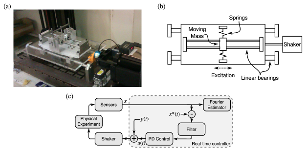
The details of the actuation and measurement equipment are as follows. The NTMD is excited using an APS-113 long-stroke electrodynamic shaker in current control mode using a Maxon ADS-50/10-4QDC motor controller. Typical base displacements are sinusoidal with a frequency ranging from $2.2$–$3.2\,\text{Hz}$ and an amplitude ranging from $0$–$25\,\text{mm}$. The peak response amplitude is limited to $\pm 80\,\text{mm}$; at resonance, this limitation restricts the amplitude of the base motion to approximately $\pm 7\,\text{mm}$. The motion of the base and the moving mass are measured using laser displacement sensors (an Omron ZX2-LD100 and an Omron ZX1-LD300 respectively). In addition to the displacement measurements, the force provided by the shaker is measured using an MCL-type load cell.

For the real-time control, a linear proportional-derivative (PD) controller is used with manually tuned gains. The methodology is relatively insensitive to the control gains used provided they are sufficient to stabilise any unstable orbits that are encountered. The controller is implemented on a BeagleBone Black fitted with a custom data acquisition board (hardware schematics and associated software are open source and freely available [27]). All measurements are made at $1\,\text{kHz}$ with no filtering.

A random perturbation signal is generated, when necessary, on the real-time control board using the Box-Muller transformation to generate Gaussian pseudo-random numbers which are then filtered using a sixth-order Butterworth filter with a cut-off arbitrarily set at $10\,\text{Hz}$ (below the Nyquist frequency of the discretisation used for Eq. (15)).

Estimations of the Fourier coefficients of the response and the control action are also calculated in real-time on the control board. However, this was for convenience rather than a necessity.

5 Experimental results

The basic control-based continuation algorithm described in Sec. 2 was used to do repeated continuations in the forcing amplitude (the amplitude of displacement of the shaking table) for fixed values of the forcing frequency. The forcing frequency, while fixed for individual continuation runs, was varied between $2.2\,\text{Hz}$ and $3.2\,\text{Hz}$ in steps of $0.025\,\text{Hz}$. At each data point, full time series measurements were made. These are shown as black dots in Fig. 3 where the forcing frequency and forcing amplitude (in mm) are plotted against the response amplitude, which we define as the magnitude of the first component in the Fourier series.

Figure 3: Measurements taken from $41$ continuation runs that vary the forcing amplitude for different fixed values of the forcing frequency. The forcing frequency is changed in steps between $2.2\,\text{Hz}$ and $3.2\,\text{Hz}$. The shaded surface is calculated using Gaussian process regression on the measured data points. The location of the unstable periodic orbits in this figure can be inferred from the geometry of the solution surface; the plotted curve (solid line) represents a 1D fold curve inside which are the unstable periodic orbits. This fold curve is calculated using the Gaussian process regressor.

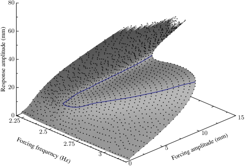
To aid visualisation, a continuous surface constructed from the individual data points is also plotted in Fig. 3. This continuous surface is created using Gaussian progress regression on the collected data points where the hyper-parameters for the Gaussian process are calculated by maximising the marginal likelihood of the hyper-parameters [28, Sec. 5.4].

The use of Gaussian process regression (or any other similar scheme for interpolating the multi-dimensional data) also allows for geometric features of the solution surface to be easily extracted. One pertinent feature is the fold in the solution surface which, from dynamical systems theory, indicates a change in stability of the periodic orbits. As such, the fold curve shown in Fig. 3 (blue curve) was extracted using numerical continuation with CoCo [20] directly on the regression surface defined by the Gaussian process.

Figure 4: A series of frequency response curves extracted from the data shown in Fig. 3 using Gaussian process regression. The forcing amplitudes of the base motion are $1.9$, $2$, $2.5$, $3$ and $3.5\,\text{mm}$ respectively. Fold points (limit points) which determine the hysteresis region are marked with black dots.

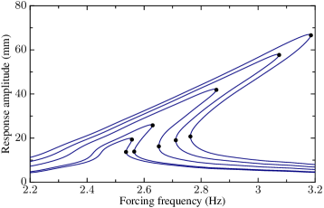
Other features of interest are frequency response curves which can also be obtained through numerical continuation on the regression surface by fixing the forcing amplitude to a prescribed value. Figure 4 shows such frequency response curves, including unstable periodic orbits, for fixed forcing amplitudes of $\Gamma=1.9$, $2$, $2.5$, $3$ and $3.5\,\text{mm}$. For high-amplitude forcing, there is little to distinguish the results to those obtained from a Duffing equation with hardening nonlinearity. However, for low-amplitude forcing there seems to be a significant influence from frictional nonlinearities in the bearing system suspending the mass.

Figure 5: Two separate time-series measurements in taken open-loop conditions starting from the same unstable periodic orbit. The measurements where synchronised using the periodic forcing as a reference signal. Noise in the experiment randomly perturbs the trajectory from the unstable periodic orbit to either the stable high-amplitude orbit (blue) or the stable low-amplitude orbit (red). This shows that the stable manifold of the unstable periodic orbit acts as a separatrix between the basins of attraction of the high- and low-amplitude orbits.

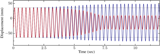
In order to verify that the unstable orbits found in the experiment are true unstable periodic orbits and not artefacts of the control scheme, we repeatedly drive the system to a particular unstable periodic orbit and then turn off the stabilising controller. As can be seen from the time series shown in Fig. 5, starting from the unstable periodic orbit both the stable low-amplitude and stable high-amplitude periodic orbits can be reached — the stable manifold of the unstable orbit acts as a separatrix between the two stable orbits as we would expect from dynamical systems theory. Out of $40$ separate time series recorded starting from the same unstable periodic orbit, $8$ end at the high-amplitude periodic orbit and the remaining end at the low-amplitude periodic orbit.

Figure 6: Panels (a) and (b) show 2D and 3D state-space projections of a single stable periodic orbit (red) and the randomly perturbed orbit (blue) used to calculate the stability of the periodic orbit. Time-delay coordinates are used as a proxy for the derivative of the position $x(t)$ to recreate the state space. The time coordinate in panel (b) is normalised such that a period of forcing takes one time unit.

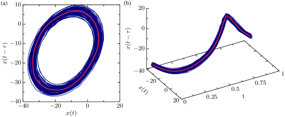
In order to apply the method outlined in Sec. 3, once an orbit has been obtained using control-based continuation it must be perturbed with a random input signal. One such example with a perturbation size of $0.5$ is shown in Fig. 6. (Strictly speaking, the perturbation size is measured in volts as it is an input to the shaker; however, the spectral content of the perturbation combined with the non-trivial frequency response of the shaker mean that it is not straightforward or useful to state the perturbation size in mm.) To avoid estimating the velocity of motion, a time-delay coordinate $x(t-\tau)$ is used to reconstruct the state-space of the experiment. Here the value of $\tau$ used is $T/5$ where $T$ is the period of the forcing.

Figure 7: The mean and $95\%$ confidence interval of the absolute values of the dominant Floquet multipliers estimated against the size of the perturbation applied. Each point represents $10$ separate measurements. The points marked (a) (red) are calculated for a stable periodic orbit in open-loop conditions; the points marked (b) (blue) are calculated for the same stable periodic orbit in closed-loop conditions; and the points marked (c) (green) are calculated for an unstable periodic orbit in closed-loop conditions. For the stable periodic orbits (a) and (b) the Floquet multipliers are complex; the estimated errors in the real and imaginary parts are approximately equal.

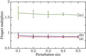
There is a single parameter in Sec. 3 for which there is no algorithmic way to determine an appropriate value, that is the amplitude of the perturbation applied to the periodic orbit. Thus in order to determine an appropriate amplitude we select two periodic orbits, one stable and one unstable and calculate the Floquet multipliers using the fitted linear time-varying model Eq. (15) for a variety of perturbation sizes and repeat the experiments $10$ times.

Throughout this paper we set $m=10$ and $n=4$ in Eq. (15).

The results of the Floquet multiplier estimations are shown in Fig. 7. The points marked (a) (in red) are the absolute values of the Floquet multipliers estimated for a stable periodic orbit while the experiment is running in open-loop; similarly, the points marked (b) (in blue) are the Floquet multipliers estimated for the same stable periodic orbit while the experiment is running in closed-loop. Finally, the points marked (c) (in green) are the Floquet multipliers estimated for an unstable periodic orbit while the experiment is running in closed-loop. Each Floquet multiplier is marked with the $95\%$ confidence range.

For both the stable and the unstable periodic orbits it can be seen that the $95\%$ confidence range narrows significantly for larger perturbation sizes; the larger perturbations allow the Floquet multipliers to be estimated more consistently. However, the consistency of the results does not imply accuracy — as with estimating derivatives from finite differences, taking a large step introduces errors caused by the nonlinearities in the system. Though, since the mean magnitude of the Floquet multipliers does not change significantly beyond a perturbation size of $0.2$, we can have reasonable confidence in the results and so a perturbation size of $0.5$ is used throughout the remainder of this paper.

Furthermore, Fig. 7 shows that running the system in closed-loop rather than open-loop does not have a significant affect on the estimation of the Floquet multipliers — the error bars of the points (a) and (b) overlap considerably.

Unfortunately no accurate independent estimations of the Floquet multipliers are available to check the results of the system identification. Convergence tests on the stable periodic orbit were performed, however the transient dynamics of the electrodynamic shaker as the experiment equilibrated rendered the results meaningless. Furthermore, escape tests from the unstable periodic orbit such as those seen in Fig. 5 produced estimates ranging from $1.2$ to $1.5$ depending on the measurement cut-offs used. As such, we consider the best way to judge the accuracy of the estimations is via comparison with geometric phenomena such as fold points where a Floquet multiplier should pass through $+1$ in the complex plane.

Figure 8: Panel (a) shows a single continuation with the response amplitude plotted against the forcing amplitude for a fixed fixed forcing frequency of $3.2\,\text{Hz}$. Stable periodic orbits are shown by solid blue dots and unstable orbits are shown by red circles. The maximum displacement of the experiment is limited to $\pm 80\,\text{mm}$. Panel (b) shows the absolute value of the estimated Floquet multipliers plotted against the response amplitude for three separate continuation runs (each shown with a different symbol). It can be seen that most of the stable periodic orbits have complex conjugate Floquet multipliers which then become real close to the saddle-node bifurcations; between the two saddle-node bifurcations, one of these Floquet multipliers lies outside the unit circle while the other lies inside the unit circle.

Subsequently, a continuation in the forcing amplitude was performed with Floquet multipliers estimated for each obtained solution; the results are shown in Fig. 8(a) with stable periodic orbits marked as solid blue dots and unstable periodic orbits marked as red circles. The results agree very well with what is expected from dynamical systems theory; the orbits between the two fold points are all unstable.

To ensure repeatability, the same continuation run was carried out three times and the absolute values of the corresponding Floquet multipliers are plotted in Fig. 8(b) with different symbols for the different runs. As can be seen from Fig. 8(b) the results are very consistent with all the runs showing good quantitative as well as qualitative agreement. As expected, a complex conjugate pair of Floquet multipliers becomes real close to the fold point after which a single real multiplier passes through the unit circle. This process reverses close to the second fold point.

Figure 9: State-space projections in 2D and 3D of the data shown in Fig. 5 using time-delay coordinates. The red curve represents the unstable periodic orbit and the two green curves represent the stable high- and low-amplitude periodic orbits. The blue curves show the transient dynamics between the unstable orbits and the stable orbits. The two different stable orbits are reached with approximately equal probability. The time coordinate in panel (b) is normalised such that a period of forcing takes one time unit.

As well as providing information about the Floquet multipliers of the periodic orbits, the monodromy matrix obtained from Eq. (15) also provides the stable and unstable eigendirections of the periodic orbit. Figure 9 shows the time series from Fig. 5 plotted in state-space, with the unstable periodic orbit (marked in red) lying between the two stable periodic orbits (marked in green). From Fig. 9(b) it can be seen that the escape from the unstable periodic orbit occurs along a two-dimensional unstable manifold.

Figure 10: A Poincaré section showing measurements from $40$ separate time series of the escape from the unstable periodic orbit shown in Fig. 5 and Fig. 9. Each dot (blue) corresponds to an intersection with the Poincaré section defined by $t\mod T=0$, where $T$ is the forcing period. The dots trace out the 1D unstable manifold of the unstable orbit. The positions of the stable high- and low-amplitude periodic orbits are marked with green crosses. The stable and unstable eigenspaces estimated using the methodology outlined in this paper are marked by red arrows. The unstable eigenspace shows good agreement with the dots from the time series measurements.

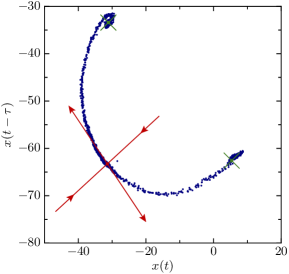
Figure 10 shows a Poincaré section at a fixed time in the forcing cycle that was created with the data from Fig. 9 combined with data from a further $38$ independent time series measurements; the blue dots denote intersections of the trajectories with the Poincaré section. The intersection of the two-dimensional unstable manifold with the Poincaré section results in a well defined one-dimensional curve showing how trajectories leave the unstable periodic orbit (marked with a red dot) and approach the two stable periodic orbits (marked with green crosses).

Superimposed on Fig. 10 is a set of red arrows which mark the unstable and stable eigendirections calculated from the monodromy matrix of the periodic orbit using only local perturbations (as previously described). The eigendirections represent the linearisation of the manifolds at the unstable periodic orbit and, as such, show remarkably good agreement with the measured unstable manifold which was calculated in open-loop conditions. This opens up the possibility for using eigendirection information in other calculations on the physical system, for example the estimation of basins of attraction.

6 Conclusions

This paper has proposed a new method for estimating Floquet multipliers and their associated eigendirections for periodic orbits that encountered when using control-based continuation on a physical experiment. A linear time-varying model in the form of an auto-regressive model with exogenous inputs (ARX) is fitted to each periodic orbit using small perturbations to the orbit to explore the nearby state-space.

The method was demonstrated on a nonlinear mass-spring-damper-type experiment that has a hardening spring characteristic. The nonlinearity is provided by placing springs perpendicular to the direction of motion, thus creating a geometric nonlinearity. The Floquet multiplier estimations were shown to agree with what is expected from dynamical systems theory and the associated eigendirections match well with open-loop measurements taken.

7 Data statement

All the experimental data used in this paper has been deposited into the University of Bristol Research Data Repository and is publicly available for download [29].

8 Acknowledgements

D.A.W.B. is supported by EPSRC First Grant EP/K032739/1. D.A.W.B also gratefully acknowledges discussions with and input from Ludovic Renson, Alicia Gonzalez-Buelga and Simon Neild.

9 References

References

- [1] K. Pyragas, Continuous control of chaos by self-controlling feedback, Physics Letters A 170 (6) (1992) 421–428. doi:10.1016/0375-9601(92)90745-8.
- [2] K. Pyragas, Control of chaos via an unstable delayed feedback controller, Physical Review Letters 86 (11) (2001) 2265–2268. doi:10.1103/PhysRevLett.86.2265.
- [3] K. Pyragas, Analytical properties and optimization of time-delayed feedback control, Physical Review E 66 (2) (2002) 026207. doi:10.1103/PhysRevE.66.026207.
- [4] J. Sieber, B. Krauskopf, Control based bifurcation analysis for experiments, Nonlinear Dynamics 51 (3) (2008) 365–377. doi:10.1007/s11071-007-9217-2.
- [5] E. Ott, C. Grebogi, J. A. Yorke, Controlling chaos, Physical Review Letters 64 (11) (1990) 1196–1199. doi:10.1103/PhysRevLett.64.1196.
- [6] S. Misra, H. Dankowicz, M. R. Paul, Event-driven feedback tracking and control of tapping-mode atomic force microscopy, Proceedings of the Royal Society A 464 (2096) (2008) 2113–2133. doi:10.1098/rspa.2007.0016.
- [7] C. I. Siettos, I. G. Kevrekidis, D. Maroudas, Coarse bifurcation diagrams via microscopic simulators: a state-feedback control-based approach, International Journal of Bifurcation and Chaos 14 (1) (2004) 207–220. doi:10.1142/S0218127404009193.
- [8] J. Sieber, A. Gonzalez-Buelga, S. A. Neild, D. J. Wagg, B. Krauskopf, Experimental continuation of periodic orbits through a fold, Physical Review Letters 100 (24) (2008) 244101. doi:10.1103/PhysRevLett.100.244101.
- [9] D. A. W. Barton, S. G. Burrow, Numerical continuation in a physical experiment: investigation of a nonlinear energy harvester, ASME Journal of Computational and Nonlinear Dynamics 6 (1) (2011) 011010. doi:10.1115/1.4002380.
- [10] D. A. W. Barton, B. P. Mann, S. G. Burrow, Control-based continuation for investigating nonlinear experiments, Journal of Vibration and Control 18 (4) (2012) 509–520. doi:10.1177/1077546310384004.
- [11] E. Bureau, F. Schilder, I. Ferreira Santos, J. Juel Thomsen, J. Starke, Experimental bifurcation analysis of an impact oscillator — tuning a non-invasive control scheme, Journal of Sound and Vibration 332 (22) (2013) 5883–5897. doi:10.1016/j.jsv.2013.05.033.
- [12] E. Bureau, F. Schilder, M. Elmegård, I. F. Santos, J. J. Thomsen, J. Starke, Experimental bifurcation analysis of an impact oscillator — determining stability, Journal of Sound and Vibration 333 (21) (2014) 5464–5474. doi:10.1016/j.jsv.2014.05.032.
- [13] D. A. W. Barton, J. Sieber, Systematic experimental exploration of bifurcations with noninvasive control, Physical Review E 87 (5) (2013) 052916. doi:10.1103/PhysRevE.87.052916.
- [14] L. Renson, A. Gonzalez-Buelga, D. A. W. Barton, S. A. Neild, Robust identification of backbone curves using control-based continuation, in press, Journal of Sound and Vibration (2015).
- [15] K. D. Murphy, P. V. Bayly, L. N. Virgin, J. A. Gottwald, Measuring the stability of periodic attractors using perturbation-induced transients: applications to two non-linear oscillators, Journal of Sound and Vibration 172 (1) (1994) 85–102. doi:10.1006/jsvi.1994.1160.
- [16] L. N. Virgin, M. D. Todd, C. J. Begley, S. T. Trickey, E. H. Dowell, Basins of attraction in experimental nonlinear oscillators, International Journal of Bifurcation and Chaos 8 (3) (1998) 521–533. doi:10.1142/S0218127498000334.
- [17] I. Kozinsky, H. W. C. Postma, O. Kogan, A. Husain, M. L. Roukes, Basins of attraction of a nonlinear nanomechanical resonator, Physical Review Letters 99 (20) (2007) 207201. doi:10.1103/physrevlett.99.207201.
- [18] R. Seydel, Practical bifurcation and stability analysis, 3rd Edition, Vol. 5 of Interdisciplinary Applied Mathematics, Springer, New York, 2010.
- [19] Y. A. Kuznetsov, Elements of applied bifurcation theory, 2nd Edition, Applied Mathematical Sciences, Springer, New York, 1998.
- [20] H. Dankowicz, F. Schilder, Recipes for continuation, SIAM, 2013. doi:10.1137/1.9781611972573.
-
[21]
E. J. Doedel, B. E. Oldeman,
AUTO-07p: continuation and
bifurcation software for ordinary differential equations, Tech. rep.,
Concordia University, Montreal (Canada 2012).
URL http://indy.cs.concordia.ca/auto/ - [22] T. Söderström, P. Stoica, System identification, Prentice Hall, 1989.
- [23] J. D. Hamilton, Time series analysis, Princeton University Press, 1994.
- [24] P. J. Brockwell, R. A. Davis, Time series: theory and methods, 2nd Edition, Springer, New York, 1991.
- [25] L. Ljung, System identification: theory for the user, 2nd Edition, Prentice Hall, 1999.
- [26] N. A. Alexander, F. Schilder, Exploring the performance of a nonlinear tuned mass damper, Journal of Sound and Vibration 319 (1–2) (2009) 445–462. doi:10.1016/j.jsv.2008.05.018.
[27]
D. A. W. Barton, Real-time control
hardware/software based on the BeagleBone Black, available online (2015).
URL http://github.com/~db9052/rtc - [28] C. E. Rasmussen, C. K. I. Williams, Gaussian processes for machine learning, MIT Press, 2006.
- [29] D. A. W. Barton, Experimental data for “Control-based continuation: bifurcation and stability analysis for physical experiments”, available online (2015). doi:10.5523/bris.1esk6h8klq0bg1gdcr78a2ypyz.