Towards Benchmarking
Scene Background Initialization

Abstract

Given a set of images of a scene taken at different times, the availability of an initial background model that describes the scene without foreground objects is the prerequisite for a wide range of applications, ranging from video surveillance to computational photography. Even though several methods have been proposed for scene background initialization, the lack of a common groundtruthed dataset and of a common set of metrics makes it difficult to compare their performance. To move first steps towards an easy and fair comparison of these methods, we assembled a dataset of sequences frequently adopted for background initialization, selected or created ground truths for quantitative evaluation through a selected suite of metrics, and compared results obtained by some existing methods, making all the material publicly available.

I Introduction

The scene background modeling process is characterized by three main tasks: 1) model representation, that describes the kind of model used to represent the background; 2) model initialization, that regards the initialization of this model; and 3) model update, that concerns the mechanism used for adapting the model to background changes along the sequence. These tasks have been addressed by several methods, as acknowledged by several surveys (e.g., [1, 2]). However, most of these methods focus on the representation and the update issues, whereas limited attention is given to the model initialization. The problem of scene background initialization is of interest for a very vast audience, due to its wide range of application areas. Indeed, the availability of an initial background model that describes the scene without foreground objects is the prerequisite, or at least can be of help, for many applications, including video surveillance, video segmentation, video compression, video inpainting, privacy protection for videos, and computational photography (see [3]).

We state the general problem of background initialization, also known as bootstrapping, background estimation, background reconstruction, initial background extraction, or background generation, as follows:

Given a set of images of a scene taken at different times, in which the background is occluded by any number of foreground objects, the aim is to determine a model describing the scene background with no foreground objects.

Depending on the application, the set of images can consist of a subset of initial sequence frames adopted for background training (e.g., for video surveillance), a set of non-time sequence photographs (e.g., for computational photography), or the entire available sequence. In the following, this set of images will be generally referred to as the bootstrap sequence.

In order to move first steps towards an easy and fair comparison of existing and future background initialization methods, we assembled and made publicly available the SBI dataset, a set of sequences frequently adopted for background initialization, including ground truths for quantitative evaluation through a selected suite of metrics, and compared results obtained by some existing methods.

II Sequences

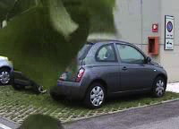
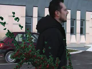
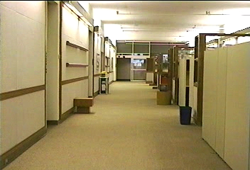
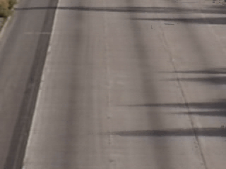
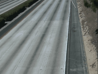
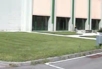
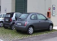
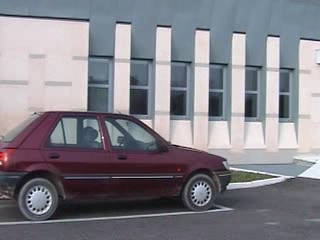
The SBI dataset includes seven bootstrap sequences extracted by original publicly available sequences that are frequently used in the literature to evaluate background initialization algorithms; example frames are shown in Fig. 1. They belong to the datasets COST 211 (sequence Hall&Monitor can be found at http://www.ics.forth.gr/cvrl/demos/NEMESIS/hall_monitor.mpg), ATON (dataset available at http://cvrr.ucsd.edu/aton/shadow/index.html), and PBI (dataset available at http://www.diegm.uniud.it/fusiello/demo/bkg/).

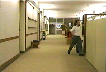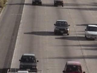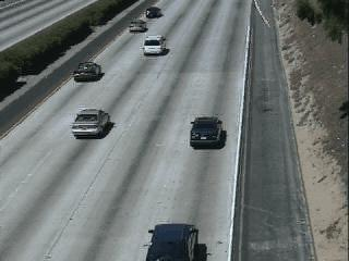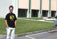frame 295	frame 0	frame 0	frame 0	frame 261	frame 10	frame 0
Hall&Monitor	HighwayI	HighwayII	CaVignal	Foliage	People&Foliage	Snellen

Figure 1: Example frames from the seven sequences of the SBI dataset (first row) and corresponding GT (second row).

In Table I we report, for each sequence, the name, the dataset it belongs to, the number of available frames, the subset of the frames adopted for testing, the original and the final resolution. The subsets have been selected in order to avoid the inclusion into the testing sequences of empty frames (frames not including foreground objects), while the final resolution has been chosen in order to avoid problems in the computation of boundary patches for block-based methods. The ground truths (GT) have been manually obtained by either choosing one of the sequence frames free of foreground objects (not included into the subsets of used frames) or by stitching together empty background regions from different sequence frames. Both the complete SBI dataset and the ground truth reference background images were made publicly available through the SBMI2015 website at http://sbmi2015.na.icar.cnr.it.

TABLE I: Information on sequences adopted for evaluation.

		Original	Used	Original	Final
Name	Dataset	frames	frames	Resolution	Resolution
Hall&Monitor	COST 211	0-299	4-299	352x240	352x240
HighwayI	ATON	0-439	0-439	320x240	320x240
HighwayII	ATON	0-499	0-499	320x240	320x240
CaVignal	PBI	0-257	0-257	200x136	200x136
Foliage	PBI	0-399	6-399	200x148	200x144
People&Foliage	PBI	0-349	0-340	320x240	320x240
Snellen	PBI	0-333	0-320	146x150	144x144

III Metrics

The metrics adopted to evaluate the accuracy of the estimated background models have been chosen among those used in the literature for background estimation. Denoting with $GT$ (Ground Truth) an image containing the true background and with $CB$ (Computed Background) the estimated background image computed with one of the background initialization methods, the eight adopted metrics are:

1. Average Gray-level Error (AGE): It is the average of the gray-level absolute difference between $GT$ and $CB$ images. Its values range in [0, $L$-1], where $L$ is the maximum number of grey levels; the lower the AGE value, the better is the background estimate.

2. Total number of Error Pixels (EPs): An error pixel is a pixel of $CB$ whose value differs from the value of the corresponding pixel in $GT$ by more than some threshold $\tau$ (in the experiments the suggested value $\tau$=20 has been adopted). EPs assume values in [$0,N$], where $N$ is the number of image pixels; the lower the EPs value, the better is the background estimate.

3. Percentage of Error Pixels (pEPs): It is the ratio between the EPs and the number $N$ of image pixels. Its values range in [0, 1]; the lower the pEPs value, the better is the background estimate.

4. Total number of Clustered Error Pixels (CEPs): A clustered error pixel is defined as any error pixel whose 4-connected neighbors are also error pixels. CEPs values range in [0, $N$]; the lower the CEPs value, the better is the background estimate.

5. Percentage of Clustered Error Pixels (pCEPs): It is the ratio between the CEPs and the number $N$ of image pixels. Its values range in [0,1]; the lower the pCEPs value, the better is the background estimate.

6. Peak-Signal-to-Noise-Ratio (PSNR): It is defined as $PSNR=10\cdot\log_{10}\left((L-1)^{2}/MSE\right),$ where $L$ is the maximum number of grey levels and MSE is the Mean Squared Error between $GT$ and $CB$ images. This frequently adopted metric assumes values in decibels (db); the higher the PSNR value, the better is the background estimate.

7. MultiScale Structural Similarity Index (MS-SSIM): This is the metric defined in [4], that uses structural distortion as an estimate of the perceived visual distortion. It assumes values in $[0,1]$; the higher the value of $MS-SSIM$, the better is the estimated background.

8. Color image Quality Measure (CQM): It is a recently proposed metric [5], based on a reversible transformation of the YUV color space and on the PSNR computed in the single YUV bands. It assumes values in db and the higher the CQM value, the better is the background estimate.

While the last metric is defined only for color images, metrics 1) through 7) are expressly defined for gray-scale images. In the case of color images, they are generally applied to either the gray-scale converted image or the luminance component Y of a color space such as YCbCr. The latter approach has been chosen for measurements reported in §IV.

Matlab scripts for computing the chosen metrics were made publicly available through the SBMI2015 website at http://sbmi2015.na.icar.cnr.it.

IV Experimental Results and Comparisons

IV-A Compared Methods

Several background initialization methods have been proposed in the literature, as recently reviewed in [3]. In this study, we compared five of them, based on different methodological schemes.

The method considered here as the baseline method is the temporal Median, that computes the value of each background pixel as the median of pixel values at the same location throughout the whole bootstrap sequence (e.g., [6, 7]). In the reported experiments on color bootstrap sequences, the temporal median is computed for each pixel as the one that minimizes the sum of $L_{\infty}$ distances of the pixel from all the other pixels.

The Self-Organizing Background Subtraction (SOBS) algorithm [8] and its spatially coherent extension SC-SOBS [9] implement an approach to moving object detection based on the neural background model automatically generated by a self-organizing method without prior knowledge about the involved patterns. For each pixel, the neuronal map consists of $n\times n$ weight vectors, each initialized with the pixel value. The whole set of weight vectors for all pixels is organized as a 2D neuronal map topologically organized such that adjacent blocks of $n\times n$ weight vectors model corresponding adjacent pixels in the image. Even though not explicitly devoted to background initialization, the method has been chosen as an example of method based on temporal statistics. Indeed, the first learning phase (usually followed by an on-line phase for moving object detection), provides an initial estimate of the background, obtained through a selective update procedure over the bootstrap sequence, taking into account spatial coherence. In the experiments, the background estimate is obtained as the result of the initial training of the software SC-SOBS (publicly available in the download section of the CVPRLab at http://cvprlab.uniparthenope.it) using for all the sequences the same default parameter values. Once the neural background model is computed, the background estimate is extracted for each pixel by choosing, among the $n^{2}$ modeling weight vectors, the one that is closest to the ground truth. Indeed, this method provides the best representation of the background that can be achieved by SC-SOBS, even though it is only applicable for comparison purposes, being based on the existence of a ground truth to compare with.

The pixel-level, non-recursive method based on subsequences of stable intensity proposed in [10] (in the following denoted as WS2006) employs a two-phase approach. Relying on the assumption that a background value always has the longest stable value, for each pixel (or image block) different non-overlapping temporal subsequences with similar intensity values (“stable subsequences”) are first selected. The most reliable subsequence, which is more likely to arise from the background, is thenchosen based on the RANSAC method. The temporal mean of the selected subsequence provides the estimated background model. For the reported experiments, WS2006 has been implemented based on [10], and parameter values have been chosen among those suggested by the authors and providing the best overall results.

In the block-level, recursive, iterative model completion technique proposed in [11] (in the following denoted as RSL2011), for each block location of the bootstrap sequence, a representative set of distinct blocks is maintained along its temporal line. The background estimation is carried out in a Markov Random Field framework, where the clique potentials are computed based on the combined frequency response of the candidate block and its neighborhood. Spatial continuity of structures within a scene is enforced by the assumption that the most appropriate block provides the smoothest response. The reported experimental results have been obtained through the related software publicly available at http://arma.sourceforge.net/background_est/.

Photomontage provides an example of method for background initialization approached as optimal labeling [12]. It is an unified framework for interactive image composition, based on energy minimization, under which various image editing tasks can be done by choosing appropriate energy functions. The cost function, minimized through graph cuts, consists of an interaction term, that penalizes perceivable seams in the composite image, and a data term, that reflects various objectives of different image editing tasks. For the specific task of background estimation, the data term adopted for achieving visual smoothness is the maximum likelihood image objective. The reported experimental results have been obtained through the related software publicly available at http://grail.cs.washington.edu/projects/photomontage/.

IV-B Qualitative and Quantitative Evaluation

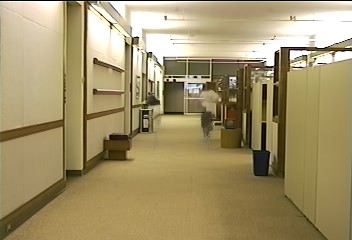
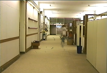
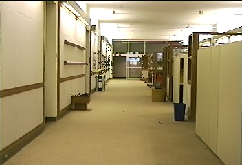
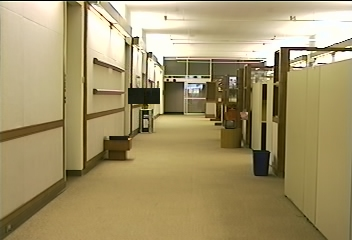
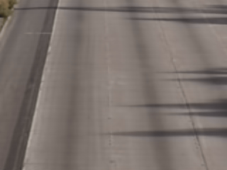
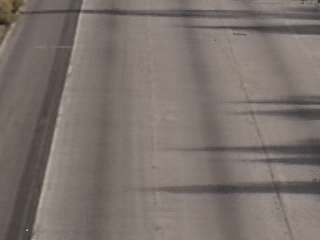
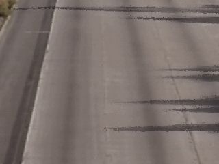
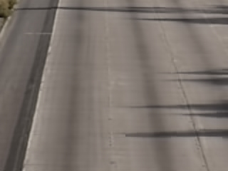
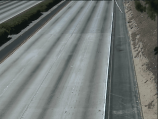
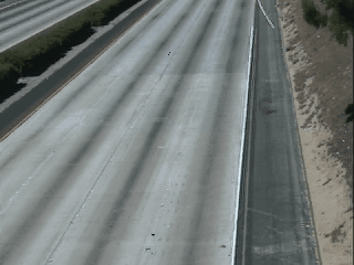
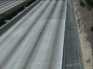
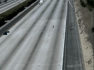
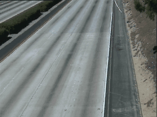
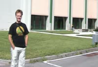
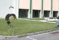
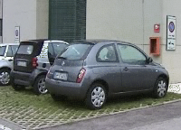
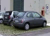
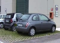
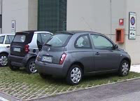
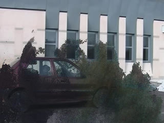
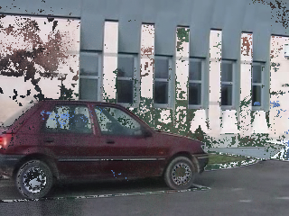
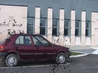
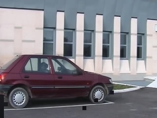
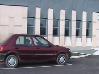
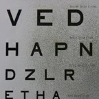
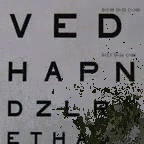
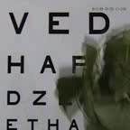
In Fig. 2 we show the background images obtained by the compared methods on the SBI dataset, while in Table II we report accuracy results according to the metrics described in §III.

For sequence Hall&Monitor, we observe few differences in initializing the background in image regions where foreground objects are more persistent during the sequence. A man walking straight down the corridor occupies the same image region for more than 65% of the sequence frames, while the briefcase is left on the small table for the last 60% of sequence frames. Only WS2006, RSL2011, and Photomontage well handle the walking man, but they include the abandoned briefcase into the background. This qualitative analysis is confirmed by accuracy results in terms of EPs and CEPs values reported in Table II. Moreover, AGE values are quite low for all the compared methods, due to the reduced size of foreground objects as compared to the image size. However, the worst AGE values are achieved by RSL2011 and Photomontage, despite their quite good qualitative results. Finally, all the compared methods achieve similar values of PSNR, MS-SSIM, and CQM, as overall, apart from reduced sized defects related to foreground objects, they all succeed in providing a sufficiently faithful representation of the empty background.

Hall&Monitor
HighwayI
HighwayII
CaVignal
Foliage
People&Foliage
Snellen
	(a)	(b)	(c)	(d)	(e)	(f)

Figure 2: Comparison of background initialization results on the SBI dataset obtained by: (a) GT, (b) Median, (c) SC-SOBS, (d) WS2006, (e) RSL2011, and (f) Photomontage

For both HighwayI and HighwayII sequences, all the compared methods succeed in providing a faithful representation of the background model. This is due to the fact that, even though the highway is always fairly crowded by passing cars, the background is revealed for at least 50% of the entire bootstrap sequence length and no cars remain stationary during the sequence. The above qualitative considerations are only partially confirmed by performance results reported in Table II. Indeed, different AGE and EPs values are achieved by qualitatively similar estimated backgrounds, while similar low CEPs values and high MS-SSIM, PSNR, and CQM values are achieved by all the compared methods.

TABLE II: Accuracy results of the compared methods on the SBI dataset.

Hall&Monitor
Method	AGE	EPs	pEPs	CEPs	pCEPs	MS-SSIM	PSNR	CQM
Median	2.7105	839	0.9931%	451	0.5339%	0.9640	30.4656	42.6705
SC-SOBS	2.4493	828	0.9801%	272	0.3220%	0.9653	30.4384	43.1867
WS2006	2.6644	470	0.5563%	26	0.0308%	0.9821	30.9313	40.0949
RSL2011	3.2687	703	0.8321%	398	0.4711%	0.9584	28.4428	37.9971
Photomontage	2.7986	305	0.3610%	69	0.0817%	0.9819	33.3715	41.7323
HighwayI
Median	1.4275	120	0.1563%	11	0.0143%	0.9924	40.1432	62.5723
SC-SOBS	1.2286	3	0.0039%	0	0.0000%	0.9949	42.6868	65.5755
WS2006	2.5185	526	0.6849%	19	0.0247%	0.9816	35.6885	56.9113
RSL2011	2.8139	267	0.3477%	33	0.0430%	0.9830	36.0290	51.9835
Photomontage	2.1745	313	0.4076%	37	0.0482%	0.9830	37.1250	59.0270
HighwayII
Median	1.7278	245	0.3190%	1	0.0013%	0.9961	34.6639	42.3162
SC-SOBS	0.6536	7	0.0091%	0	0.0000%	0.9982	44.6312	54.3785
WS2006	2.4906	375	0.4883%	10	0.0130%	0.9927	33.9515	40.5088
RSL2011	5.6807	956	1.2448%	316	0.4115%	0.9766	28.6703	35.0821
Photomontage	2.4306	452	0.5885%	4	0.0052%	0.9909	34.3975	41.7656
CaVignal
Median	10.3082	2846	10.4632%	2205	8.1066%	0.7984	18.1355	33.1438
SC-SOBS	4.0941	869	3.1949%	436	1.6029%	0.8779	21.8507	42.2652
WS2006	2.5403	408	1.5000%	129	0.4743%	0.9289	27.1089	37.0609
RSL2011	1.6132	4	0.0147%	0	0.0000%	0.9967	41.3795	52.5856
Photomontage	11.2665	3052	11.2206%	2408	8.8529%	0.7919	17.6257	32.0570
Foliage
Median	27.0135	13626	47.3125%	8772	30.4583%	0.6444	16.7842	28.7321
SC-SOBS	3.8215	160	0.5556%	0	0.0000%	0.9900	31.7713	39.1387
WS2006	6.8649	821	2.8507%	2	0.0069%	0.9754	27.2438	34.9776
RSL2011	2.2773	43	0.1493%	11	0.0382%	0.9951	36.7450	43.1208
Photomontage	1.8592	0	0.0000%	0	0.0000%	0.9974	39.1779	45.6052
People&Foliage
Median	24.4211	24760	32.2396%	19446	25.3203%	0.6114	15.1870	27.4979
SC-SOBS	15.1031	10770	14.0234%	3849	5.0117%	0.7561	16.6189	35.3667
WS2006	5.4243	2743	3.5716%	71	0.0924%	0.9269	22.6952	31.3847
RSL2011	2.0980	612	0.7969%	434	0.5651%	0.9905	32.5550	37.0598
Photomontage	1.4103	3	0.0039%	0	0.0000%	0.9973	41.0866	47.1517
Snellen
Median	42.3981	12898	62.2010%	11814	56.9734%	0.6932	13.6573	36.0691
SC-SOBS	16.8898	7746	37.3553%	5055	24.3779%	0.9303	21.2571	44.7498
WS2006	23.0010	4804	23.1674%	2544	12.2685%	0.7481	15.6158	24.9930
RSL2011	1.8095	133	0.6414%	99	0.4774%	0.9979	38.0295	50.2600
Photomontage	29.9797	6946	33.4973%	6318	30.4688%	0.5926	14.1466	26.9210

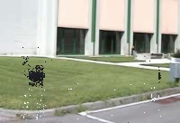
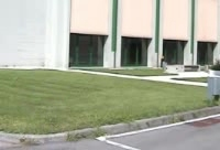
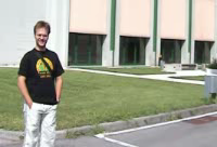
Sequence CaVignal represents a major burden for most of the compared methods. Indeed, the only man appearing in the sequence stands still on the left of the scene for the first 60% of sequence frames; then starts walking and rests on the right of the scene for the last 10% of sequence frames. The persistent clutter at the beginning of the scene leads most of the compared methods to include the man on the left into the estimated background, while the persistent clutter at the end of the scene leads only WS2006 to partially include the man on the right into the background. Only RSL2011 perfectly handles the persistent clutter, accordingly achieving the best accuracy results for all the metrics.

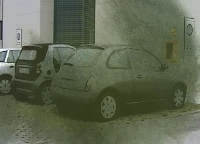
For sequence Foliage, even though moving leaves occupy most of the background area for most of the time, many of the compared methods achieve a quite good representation of the scene background. Indeed, only Median produces a greenish halo due to the foreground leaves over almost the entire scene area, and accordingly achieves the worst accuracy results for all the metrics.

Also sequence People&Foliage is problematic for most of the compared methods. Indeed, the artificially added leaves and men occupy almost all the scene area in almost all the sequence frames. Only Photomontage and RSL2011 appear to well handle the wide clutter, also achieving the best accuracy results for all the metrics.

In sequence Snellen, the foreground leaves occupy almost all the scene area in almost all the sequence frames. This leads most of the methods to include the contribution of leaves into the final background model. The best qualitative result can be attributed to RSL2011, as confirmed by the quantitative analysis in terms of all the adopted metrics.

Overall, we can observe that most of the best performing background initialization methods are region-based or hybrid, confirming the importance of taking into account spatio-temporal inter-pixel relations. Also selectivity in choosing the best candidate pixels, shared by all the best performing methods, appears to be important for achieving accurate results. Instead, all the common methodological schemes shared by the compared methods can lead to accurate results, showing no preferred scheme, and the same can be said concerning recursivity.

In order to assess the challenge that each sequence poses for the tested methods, we further computed the median values of all metrics obtained by the compared methods for each sequence, and ranked the sequences according to these median values, as shown in Table III. Here, HighwayI and HighwayII sequences reveal as those that are best handled by all methods (in the sense of median), while Snellen is the worst handled. Bearing in mind the kind of foreground objects included into the sequences, we can observe that their size is not a major burden; e.g., Foliage sequence is better handled than Hall&Monitor, even though the size of the foreground objects is much larger. Instead, their speed (or their steadiness) has much greater influence on the results. As instance, CaVignal sequence is worse handled than Foliage, since it includes almost static foreground objects that are frequently misinterpreted as background. It can also be observed that the median values of pEPs and MS-SSIM metrics perfectly vary according to the difficulty in handling the sequences; these two metrics confirm to be strongly indicative of the performance of background initialization methods.

TABLE III: Median values of all metrics obtained by the compared methods for each sequence and average rank of the sequences according to these median values.

Sequence	Av.	Median	Median	Median	Median	Median	Median	Median	Median
	rank	AGE	EPs	pEPs	CEPs	pCEPs	MS-SSIM	PSNR	CQM
HighwayI	1,63	2,17	267	0,35%	19	0,02%	0,97	37,13	59,03
HighwayII	2,00	2,43	375	0,49%	4	0,01%	0,95	34,40	41,77
Foliage	2,50	3,82	160	0,56%	2	0,01%	0,95	31,77	39,14
Hall&Monitor	3,75	2,71	703	0,83%	272	0,32%	0,95	30,47	41,73
CaVignal	5,63	4,09	956	3,19%	435	1,60%	0,89	21,85	35,08
People&Foliage	5,63	5,42	2743	3,57%	434	0,57%	0,78	22,70	35,37
Snellen	6,75	23,00	6946	33,50%	5055	24,38%	0,76	15,62	36,07

V Concluding Remarks

We proposed a benchmarking study for scene background initialization, moving the first steps towards a fair and easy comparison of existing and future methods, on a common dataset of groundtruthed sequences, with a common set of metrics, and based on reproducible results. The assembled SBI dataset, the ground truths, and a tool to compute the suite of metrics were made publicly available.

Based on the benchmarking study, first considerations have been drawn.

Concerning main issues in background initialization, low speed (or steadiness), rather than great size, of foreground objects included into the bootstrap sequence is a major burden for most of the methods.

All the common methodologies shared by the compared methods can lead to accurate results, showing no preferred scheme, and the same can be said concerning recursivity. Anyway, the best results are generally achieved by methods that are region-based or hybrid, and selective; thus, these are the methods to be preferred.

Another conclusion can be drawn, concerning the evaluation of background initialization methods. Among the eight selected metrics frequently adopted in the literature, pEPs and MS-SSIM confirm to be strongly indicative of the performance of background initialization methods. This can be of peculiar interest for evaluating future background initialization methods.

References

- [1] T. Bouwmans, “Traditional and recent approaches in background modeling for foreground detection: An overview,” Computer Science Review, vol. 11–12, pp. 31–66, 2014.
- [2] S. Elhabian, K. El Sayed, and S. Ahmed, “Moving object detection in spatial domain using background removal techniques: State-of-art,” Recent Patents on Computer Science, vol. 1, no. 1, pp. 32–54, Jan. 2008.
- [3] L. Maddalena and A. Petrosino, “Background model initialization for static cameras,” in Background Modeling and Foreground Detection for Video Surveillance, T. Bouwmans, F. Porikli, B. H ferlin, and A. Vacavant, Eds. Chapman & Hall/CRC, 2014, pp. 3–1–3–16.
- [4] Z. Wang, E. Simoncelli, and A. Bovik, “Multiscale structural similarity for image quality assessment,” in Signals, Systems and Computers, 2004. Conference Record of the Thirty-Seventh Asilomar Conference on, vol. 2, 2003, pp. 1398–1402 Vol.2.
- [5] Y. Yalman and I. Erturk, “A new color image quality measure based on YUV transformation and PSNR for human vision system,” Turkish J. of Electrical Eng. & Comput. Sci., vol. 21, pp. 603–612, 2013.
- [6] B. Gloyer, H. K. Aghajan, K.-Y. Siu, and T. Kailath, “Video-based freeway-monitoring system using recursive vehicle tracking,” pp. 173–180, 1995.
- [7] L. Maddalena and A. Petrosino, “The 3dSOBS+ algorithm for moving object detection,” Comput. Vis. Image Underst., vol. 122, pp. 65–73, 2014.
- [8] ——, “A self-organizing approach to background subtraction for visual surveillance applications,” IEEE Trans. Image Process., vol. 17, no. 7, pp. 1168–1177, July 2008.
- [9] ——, “The SOBS algorithm: What are the limits?” in Proc. CVPR Workshops, June 2012, pp. 21–26.
- [10] H. Wang and D. Suter, “A novel robust statistical method for background initialization and visual surveillance,” in Proc. ACCV’06. Berlin, Heidelberg: Springer-Verlag, 2006, pp. 328–337.
- [11] V. Reddy, C. Sanderson, and B. C. Lovell, “A low-complexity algorithm for static background estimation from cluttered image sequences in surveillance contexts,” EURASIP J. Image Video Process., vol. 2011, pp. 1:1–1:14, Jan. 2011.
- [12] A. Agarwala, M. Dontcheva, M. Agrawala, S. Drucker, A. Colburn, B. Curless, D. Salesin, and M. Cohen, “Interactive digital photomontage,” ACM Trans. Graph., vol. 23, no. 3, pp. 294–302, Aug. 2004.