The growth rate of the tunnel number of m-small knots

Abstract.

In [12] the authors defined the growth rate of the tunnel number of knots, an invariant that measures that asymptotic behavior of the tunnel number under connected sum. In this paper we calculate the growth rate of the tunnel number of m-small knots in terms of their bridge indices.

Part I Introduction and background material

1. Introduction

Let $M$ be a compact connected orientable 3-manifold and $K\subset M$ a knot. $K$ is called admissible if $g(E(K))>g(M)$ and inadmissible otherwise (throughout this paper $E(\cdot)$ denotes knot exterior and $g(\cdot)$ denotes the Heegaard genus; see Section 2 for these and other basic definitions). Let $nK$ denote the connected sum of $n$ copies of $K$. In [12] the authors defined the growth rate of the tunnel number of $K$ to be:

$$\mbox{gr}_{t}(K)=\limsup_{n\to\infty}\frac{g(E(nK))-ng(E(K))+n-1}{n-1}$$

The main result of [12] shows that if $K$ is admissible then $\mbox{gr}_{t}(K)<1$, and $\mbox{gr}_{t}(K)=1$ otherwise. This concept was the key to constructing a counterexample to Morimoto’s Conjecture [15] and [14]. Unless explicitly stated otherwise, all knots considered are assumed to be admissible (note that this is always the case for knots in the three sphere $S^{3}$).

In this paper we continue our investigation of the growth rate of the tunnel number. In Part 2 we give an upper bound on the growth rate of admissible knots (this is an improvement of the bound given in [12]), and in Part 3 we obtain a lower bound on the growth rate of admissible m-small knots (a knot is called m-small if its meridian is not a boundary slope of an essential surface). With this we obtain an exact calculation of the growth rate of m-small knots. Before stating this result we define the following notation that will be used extensively throughout the paper:

Notation 1.1.

Let $K\subset M$ be an admissible knot. We denote $g(E(K))-g(M)$ by $g$ and for $i=1,\dots,g$ we denote the bridge index of $K$ with respect to Heegaard surfaces of genus $g(E(K))-i$ by $b_{i}^{*}$. That is, $b_{i}^{*}$ is the minimal integer so that $K$ admits a $b_{i}^{*}$ bridge position with respect to some Heegaard surface of $M$ of genus $g(E(K))-i$; we call such a decomposition a $(g(E(K))-i,b^{*}_{i})$ decomposition. Note that for a knot $K\subset S^{3}$ we have that $g=g(E(K))$, $b_{g}^{*}(K)$ is the bridge index of $K$, and $b_{g-1}^{*}(K)$ is the torus bridge index of $K$. We note that, for any knot $K\subset M$, $b_{i}^{*}$ forms an increasing sequence of positive integers: $0<b_{1}^{*}<\cdots<b_{g}^{*}$. To see this, fix $i\geq 1$ and let $\Sigma$ be a Heegaard surface that realizes the bridge index $b_{i}^{*}$, that is, $\Sigma$ is a genus $g(E(K))-i$ Heegaard surface for $M$ with respect to which $K$ has bridge index $b_{i}^{*}$. By tubing $\Sigma$ once (see Definition 5.3) we obtain a Heegaard surface of genus $g(E(K))-(i-1)$ that realizes a $(g(E(K))-(i-1),b_{i}^{*}-1)$ decomposition for $K$. This shows that $b_{i-1}^{*}\leq b_{i}^{*}-1$.

We are now ready to state:

Theorem 1.2.

Let $M$ be a compact connected orientable 3-manifold and $K\subset M$ be an admissible knot. Then $\mbox{gr}_{t}(K)\leq\min_{i=1,\dots,g}\big{\{}1-\frac{i}{b_{i}^{*}}\big{\}}$. If, in addition, $K$ is m-small then equality holds:

$$\mbox{gr}_{t}(K)=\min_{i=1,\dots,g}\bigg{\{}1-\frac{i}{b_{i}^{*}}\bigg{\}}$$

Moreover, for m-small knots the limit of  $\frac{g(E(nK))-ng(E(K))+n-1}{n-1}$ exists.

As noted in Notation 1.1, the indices $b_{i}^{*}$ form an increasing series of positive integers. It follows that $b_{i}^{*}\geq i$; moreover, $b_{i}^{*}=i$ implies that $b_{1}^{*}=1$. Applying this to an index $i$ that realizes that the equality $\mbox{gr}_{t}(K)=1-\frac{i}{b_{i}^{*}}$ we obtain the following simple and useful consequence of Theorem 1.2 that strengthens the main result of [12] in the case of m-small knots:

Corollary 1.3.

If $K\subset M$ is an admissible m-small knot, then

$$0\leq\mbox{gr}(K)<1$$

Moreover, $\mbox{gr}(K)=0$ if and only if $b_{1}^{*}=1$.

There are several results about the spectrum of the growth rate and we summarize them here. It is well known that there exist manifolds $M$ that admit minimal genus Heegaard splittings $\Sigma$ of genus at least 2 and of Hempel distance at least 3. We fix such $M$ and $\Sigma$ and for simplicity we assume that $M$ is closed. Let $C$ be a handlebody obtained by cutting $M$ along $\Sigma$ and $K$ a core of $C$, that is, $K$ is a core of a solid torus obtained by cutting $C$ along appropriately chosen meridian disks. Then $\Sigma$ is a Heegaard surface for $E(K)$; it follows that $K$ is inadmissible. Clearly, the Hempel distance does not go down after drilling $K$. Hence the Hempel distance of $\Sigma\subset E(K)$ is at least 3. It is a well known consequence of Thurston-Perelman’s Geometrization Theorem that manifolds that admit a Heegaard surface of genus at least 2 and Hempel distance at least 3 are hyperbolic. Thus $K\subset M$ is a hypebolic knot in a hyperbolic manifold. As mentioned above, the growth rate of inadmissible knots is 1. This proves existence of hyperbolic knots in hyperbolic manifolds with growth rate 1. It was shown in [12] that torus knots and 2-bridge knots have growth rate 0. Kobayashi and Saito [16] constructed knots with growth rate $-1/2$. Theorem 1.2 enables us to calculate the growth rate of the knots constructed by Morimoto, Sakuma and Yokota in [20] (perhaps with finitely many exceptions), which we denote by $K_{MSY}$. We explain this here. The knots $K_{MSY}$ enjoy the following properties:

1. $K_{MSY}$ are hyperbolic and m-small: this was announced by by Morimoto in a preprint available at [19].

2. $g(E(K_{MSY}))=2$: this was proved by Morimoto, Sakuma, and Yokota [20].

3. $b_{1}^{*}(K_{MSY})=2$ (in other words, the torus bridge index of $K_{MSY}$ is 2): it was shown in [20] that $b_{1}^{*}>1$, and it is easy to observe that $b_{1}^{*}\leq 2$ (see, for example, [12]).

4. $b_{2}^{*}(K_{MSY})\geq 4$ (in other words, the bridge index of $K_{MSY}$ is at least 4): since $b_{2}^{*}(K_{MSY})>b_{1}^{*}(K_{MSY})$, we only need to exclude the possibility $b_{2}^{*}(K_{MSY})=3$. Assume for a contradiction that $b_{2}^{*}(K_{MSY})=3$. Then $K_{MSY}$ is a tunnel number 1, 3-bridge knot. Kim [10] proved that every tunnel number 1, 3-bridge knot has torus bridge index 1, contradicting the previous point. Recently R Bowman, S Taylor and A Zupan [2] showed that $b_{2}^{*}(K_{MSY})=7$ for all but finitely many of the knots $K_{MSY}$ (see Remak 1.6).

Using these facts, Theorem 1.2 implies that $\mbox{gr}_{t}(K_{MSY})=1/2$. This is the first example of knots with growth rate in the open interval $(0,1)$ and provides partial answer to questions posed in [12]. In summary we have the following; we emphasize that only (4) is new:

Corollary 1.4.

The following holds:

1. There exist hyperbolic knots in hyperbolic manifolds with growth rate 1.

2. There exist hyperbolic knots in $S^{3}$ with growth rate 0.

3. There exist knots in $S^{3}$ with growth rate -1/2.

4. There exist hyperbolic knots in $S^{3}$ with growth rate 1/2.

Remark 1.5.

In [1] K Baker and the authors use Theorem 1.2 to show that for any $\epsilon>0$ there exists a hyperbolic knot $K\subset S^{3}$ with $1-\epsilon<\mbox{gr}_{t}(K)<1$. This implies, in particular, that the spectrum of the growth rate is infinite.

Remark 1.6.

We take this opportunity to mention a few recent results about $b_{i}^{*}$ that appeared since we first started writing this paper; for precise statements see references.

1. In [6], given positive integers $g_{M}<i\leq g_{K}$ and $n$, K Ichihara and T Saito constructed manifolds $M$ and knots $K\subset M$ so that $g(M)=g_{M}$, $g(E(K))=g_{K}$, and $b_{i}^{*}(K)-b_{i-1}^{*}(K)\geq 2$ (see [6, Corolloar 2]; the notation there is different from ours); their arguments can easily be applied to construct knots such that $b_{i}^{*}(K)-b_{i-1}^{*}(K)\geq n$ (informally, we may phrase this as an arbitrarily large gap).

2. In [28] Zupan studies the bridge indices of iterated torus knots showing, in particular, that there exist iterated torus knots realizing arbitrarily large gaps between $b_{i-1}^{*}$ and $b_{i}^{*}$ for any $i$ in the range where both indices are defined. An easy argument shows that iterated torus knots are m-small; every knot $K$ considered by Zupan fulfils $b_{1}^{*}(K)=1$, and so has $\mbox{gr}(K)=0$ by Corollary 1.3.

3. In [2] Bowman, Taylor, and Zupan calculate the bridge indices of generic iterated torus knots (see [2] for definitions). They give conditions on the parameters that imply that $b_{g}^{*}=p$, where here the knot considered is obtained by twisting the torus knot $T_{p,q}$, $p<q$. (We note that for twisted torus knot $g=2$). Applying this to $K_{MSY}$ we see that all but finitely many of these knots have $b_{2}^{*}=7$, improving on our estimate $b_{2}^{*}\geq 4$. We remark that in [2] linear lower bound on $b_{1}^{*}$ was also obtained, showing that many twisted torus knots have a gap between $b_{1}^{*}$ and $b_{2}^{*}$; since $b_{2}^{*}$ can be made arbitrarily large, this can be seen as a second gap.

Before describing the structure and contents of this paper in more detail we introduce some necessary concepts. Let $\Sigma$ be a Heegaard surface of a compact 3-manifold $M$, and $A$ an essential annulus properly embedded in $M$. The annulus $A$ is called a Haken annulus for $\Sigma$ (Definition 4.1) if it intersects $\Sigma$ in a single simple closed curve that is essential in $A$. For an integer $c\geq 0$, the manifold obtained by drilling $c$ curves simultaneously parallel to meridians of $K$ out of $E(K)$ is denoted by $E(K)^{(c)}$ (note that $E(K)^{(0)}=E(K)$). The $c$ tori $\partial E(K)^{(c)}\setminus\partial E(K)$ are denoted by $T_{1},\dots,T_{c}$. There are $c$ annuli properly embedded disjointly in $E(K)^{(c)}$, denoted by $A_{1},\dots,A_{c}$, so that one component of $\partial A_{i}$ is a meridian on $\partial E(K)$ and the other is a longitude of $T_{i}$ ($i=1,\dots,c$). (We note that in general these annuli are not uniquely determined up to isotopy.) Annuli with these properties are called a complete system of Hopf annuli (Definition 5.1). Let $\Sigma$ be a Heegaard surface for $E(K)^{(c)}$. The Hopf annuli $A_{1},\dots,A_{c}$ are called a complete system of Hopf–Haken Annuli for $\Sigma$ (Definition 5.2) if $\Sigma\cap A_{i}$ is a single simple closed curve that is essential in $A_{i}$ ($i=1,\dots,c$).

Part 2 starts with Section 4 where we describe basic behavior of Haken annuli under amalgamation. In Section 5 we consider $(g^{\prime},b)$ decomposition of $K$ (that is, $b$-bridge decomposition of $K$ with respect to a genus $g^{\prime}$ Heegaard surface) and relate it to existence of Hopf Haken Annuli. Specifically, we prove that $K$ admits a $(g(E(K))-c,c)$ decomposition if and only if $E(K)^{(c)}$ admits a complete system of Hopf Haken Annuli for some Heegaard surface of genus $g(E(K))$ (Theorem 5.4).

In Section 6 we prove that given knots $K_{1},\dots,K_{n}$ and integers $c_{1},\dots,c_{n}\geq 0$ with $\sum_{i=1}^{n}c_{i}=n-1$, $E(K_{1}\#\cdots\#K_{n})$ admits a system of $n-1$ essential tori $\mathcal{T}$ (called swallow follow tori) so that the components of $E(K_{1}\#\cdots\#K_{n})$ cut open along $\mathcal{T}$ are homeomorphic to $E(K_{1})^{(c_{1})},\dots,E(K_{n})^{(c_{n})}$. By amalgamating Heegaard surfaces of $E(K_{1})^{(c_{1})},\dots,E(K_{n})^{(c_{n})}$ along the tori of $\mathcal{T}$ we obtain a Heegaard surface for $E(K_{1}\#\cdots\#K_{n})$; this implies the following special case of Corollary 6.4:

$$g(E(K_{1}\#\cdots\#K_{n}))\leq\sum_{i=1}^{n}g(E(K_{i})^{(c_{i})})-(n-1)$$

In the final section of Part 2, Section 7, we combine these facts to prove that for each $i$ we have:

$$\mbox{gr}_{t}(K)\leq 1-i/b_{i}^{*}$$

Thus we obtain the upper bound stated in Theorem 1.2.

To some degree, Part 3 complements Part 2. We begin with Section 8 that complements Sections 4 and 5. As mentioned above, in Sections 4 and 5 we prove that $K$ admits a $(g(E(K))-c,c)$ decomposition if and only if $E(K)^{(c)}$ admits a complete system of Hopf Haken Annuli for some Heegaard surface of genus $g(E(K))$. We are now ready to state the Strong Hopf Haken Annulus Theorem, which generalise the Hopf Haken Annulus Theorem (Theorem 6.3 of [13]) is one of the highlights of this work. The proof is given in Section 8. For the definition of a Heegaard splitting of $(N;F_{1},F_{2})$ (where $N$ is a manifold and $F_{1}$, $F_{2}$ are partitions of some of the components of $\partial N$), see Section 2 .

Theorem 1.7 (Strong Hopf-Haken Annulus Theorem).

For $i=1,\dots,n$, let $M_{i}$ be a compact connected orinetable 3-manifold and $K_{i}\subset M_{i}$ a knot. Suppose $E(K_{i})\not\cong T^{2}\times I$, $E(K_{i})$ is irreducible, and $\partial N(K_{i})$ is incompressible in $E(K_{i})$. Let $F_{1}$, $F_{2}$ be a partition of some of the components of $\partial M$, where $M=\#_{i=1}^{n}M_{i}$. Let $c\geq 0$ be an integer. Then one of the following holds:

1. There exist a minimal genus Heegaard surface for $(E(\#_{i=1}^{n}K_{i})^{(c)};F_{1},F_{2})$ admitting a complete system of Hopf–Haken annuli.

2. For some $1\leq i\leq n$, $E(K_{i})$ admits an essential meridional surface $S$ with $\chi(S)\geq 6-2g(E(\#_{i=1}^{n}K_{i})^{(c)};F_{1},F_{2})$.

One curious consequence of Theorem 1.7 (which is proved in Section 8) is the following, where $b_{g}^{*}$ is as in Notation 1.1:

Corollary 1.8.

Let $K\subset S^{3}$ be a connected sum of m-small knots. Then for $c\geq b_{g}^{*}$,

$$g(E(K)^{(c)})=c$$

Section 9 complements Section 6. Recall that in Section 6 we used swallow follow tori to show that given any collection of integers $c_{1},\dots,c_{n}\geq 0$ whose sum is $n-1$ we have that $g(E(K_{1}\#\cdots\#K_{n}))\leq\sum_{i=1}^{n}g(E(K_{i})^{(c_{i})})-(n-1)$. In Section 9 we prove that if $K_{i}$ is m-small for each $i$, then any Heegaard splitting for $E(K_{1}\#\cdots\#K_{n})$ admits an iterated weak reduction to $n-1$ swallow follow tori. This implies that any minimal genus Heegaard splitting admits an iterated weak reduction to some $n-1$ swallow follow tori that decompose $E(K_{1}\#\cdots\#K_{n})$ as $E(K_{1})^{(c_{1})},\dots,E(K_{n})^{(c_{n})}$, giving some integers $c_{1},\dots,c_{n}\geq 0$ whose sum is $n-1$. The integers $c_{1},\dots,c_{n}$ are very special (see Example 9.3).

In Section 10, which complements Section 7, we combine these results to give a lower bound on the growth rate of the tunnel number of m-small knots. Given $K$, we “expect” that $g(E(K)^{(c)})=g(E(K))+c$; we define the function ${f_{K}}$ that measures to what extent $g(E(K)^{(c)})$ fails to behave “as expected”:

$${f_{K}}(c)=g(E(K))+c-g(E(K)^{(c)})$$

For any knot $K$ and any integer $c\geq 0$, we show that ${f_{K}}$ fulfills:

$${f_{K}}(0)=0\mbox{ and }{f_{K}}(c)\leq{f_{K}}(c+1)\leq{f_{K}}(c)+1$$

We study ${f_{K}}$ for m-small knots, calculating it exactly in terms of the bridge indices of $K$ (Proposition 10.4). In particular, for m-small knots ${f_{K}}$ is bounded. In fact, for large enough $c$ Proposition 10.4 implies:

$${f_{K}}(c)=g(E(K))-g(M)$$

We do not know much about the behavior of ${f_{K}}$ in general; for example, we do not know if there exists a knot for which ${f_{K}}$ is unbounded (see Question 10.5).

We express the growth rate of tunnel number of $m$-small knots in terms of ${f_{K}}$ by showing (Corollary 10.3) that:

$$\frac{g(E(nK))-ng(E(K))+n-1}{n-1}=1-\frac{\max\{\sum_{i=1}^{n}{f_{K}}(c_{i})\}}{n-1}$$

where the maximum is taken over all collections of integers $c_{1},\dots,c_{n}\geq 0$ whose sum is $n-1$. The growth rate is then the limit superior of this sequence. We combine this interpretation of the growth rate with the calculation of ${f_{K}}$ to obtain the exact calculation of the growth rate of m-small knots stated in Theorem 1.2.

Acknowledgements. We thank Mark Arnold and Jennifer Schultens for helpful correspondence.

2. Preliminaries

By manifold we mean a smooth 3 dimensional manifold. All manifolds considered are assumed to be connected orientable and compact. We assume the reader is familiar with the basic terms of 3-manifold topology (see for example [5] or [7]). Thus we assume the reader is familiar with terms such as compression, boundary compression, boundary parallel, and essential surface.

We use the notation $\partial$, cl, and int denote boundary, closure, and interior, respectively. For a submanifold $H$ of a manifold $M$, $N(H,M)$ denotes a closed regular neighborhood of $H$ in $M$. When $M$ is understood from context we often abbreviate $N(H,M)$ to $N(H)$.

By a knot $K$ in a 3-manifold $M$ we mean a smooth embedding of $S^{1}$ into $M$, taken up to ambient isotopy. The exterior of $K$, $E(K)$, is $\mbox{cl}(M\setminus N(K))$. The slope on the torus $\partial E(K)\setminus\partial M=\partial N(K)$ that bounds a disk in $N(K)$ is called the meridian of $K$. A knot $K$ is called m-small if there is no essential meridional surface in $E(K)$, that is, there is no essential surface $S\subset E(K)$ with non empty boundary so that $\partial S$ consists of meridians of $K$.

We assume the reader is familiar with the basic terms regarding Heegaard splittings, such as handlebody, compression body, meridian disk, etc. Recall that a compression body $C$ is a connected 3-manifold obtained from $F\times[0,1]$ (where here $F$ is a possibly empty disjoint union of closed surfaces) and a (possibly empty) collection of 3-balls by attaching 1-handles to $F\times\{1\}$ and the boundary of the balls. Following standard conventions, we refer to $F\times\{0\}$ as $\partial_{-}C$ and $\partial C\setminus\partial_{-}C$ as $\partial_{+}C$. We use the notation $C_{1}\cup_{\Sigma}C_{2}$ for the Heegaard splitting given by the compression bodies $C_{1}$ and $C_{2}$. The basic concepts of reductions of a Heegaard splitting are summarized here:

Definitions 2.1.

1. A Heegaard splitting $C_{1}\cup_{\Sigma}C_{2}$ is called stabilized if there exist meridian disks $D_{1}\subset C_{1}$ and $D_{2}\subset C_{2}$ such that $\partial D_{1}$ intersects $\partial D_{2}$ transversely (as submanifolds of $\Sigma$) in one point. Otherwise, the Heegaard splitting is called non-stabilized.

2. A Heegaard splitting $C_{1}\cup_{\Sigma}C_{2}$ is called reducible if there exist meridian disks $D_{1}\subset C_{1}$ and $D_{2}\subset C_{2}$ such that $\partial D_{1}=\partial D_{2}$. Otherwise, the Heegaard splitting is called irreducible.

3. A Heegaard splitting $C_{1}\cup_{\Sigma}C_{2}$ is called weakly reducible if there exist meridian disks $D_{1}\subset C_{1}$ and $D_{2}\subset C_{2}$ such that $\partial D_{1}\cap\partial D_{2}=\emptyset$. Otherwise the splitting is called strongly irreducible.

4. A Heegaard splitting $C_{1}\cup_{\Sigma}C_{2}$ is called trivial if $C_{1}$ or $C_{2}$ is a trivial compression body, that is, a compression body with no 1-handles. Otherwise the Heegaard splitting is called non-trivial.

Let $C_{1}\cup_{\Sigma}C_{2}$ be a weakly reducible Heegaard splitting of a manifold $M$. Let $\Delta_{i}\subset C_{i}$ be a non empty set of disjoint meridian disks so that $\Delta_{1}\cap\Delta_{2}=\emptyset$. By waek reduction along $\Delta_{1}\cup\Delta_{2}$ we mean the (possibly disconnected) surface obtained by first compressing $\Sigma$ along $\Delta_{1}\cup\Delta_{2}$, and then removing any component that is contained in $C_{1}$ or $C_{2}$. Casson and Gordon [3] showed that if an irreducible Heegaard splitting is weakly reducible, then an appropriately chosen weak reduction yields a (possibly disconnected) essential surface, say $F$.

With $F$ as in the previous paragraph, let $M_{1},\dots,M_{k}$ be the components of $M$ cut open along $F$. It is well known that $\Sigma$ induces a Heegaard surface on each $M_{i}$, say $\Sigma_{i}$. We say that $\Sigma$ is obtained by amalgamating $\Sigma_{1},\dots,\Sigma_{k}$. This is a special case of amalgamation; the general definition will be given below as the converse of iterated weak reduction. The genus after amalgamation is given in the following lemma; see Remark 2.7 of [26] for the case $m=1$ (we leave the proof of the general case to the reader):

Lemma 2.2.

Let $C_{1}\cup_{\Sigma}C_{2}$ be a weakly reducible Heegaard splitting and suppose that after weak reduction we obtain $F$ (as above). Suppose that $M$ cut open along $F$ consists of two components, and denote the induced Heegaard splittings by $C_{1}^{(1)}\cup_{\Sigma_{1}}C_{2}^{(1)}$ and $C_{1}^{(2)}\cup_{\Sigma_{2}}C_{2}^{(2)}$. Let $F_{1},\dots,F_{m}$ be the components of $F$. Then

$$g(\Sigma)=g(\Sigma_{1})+g(\Sigma_{2})-\sum_{i=1}^{m}g(F_{i})+(m-1)$$

In particular, if $F$ is connected then $g(\Sigma)=g(\Sigma_{1})+g(\Sigma_{2})-g(F)$.

It is distinctly possible that not all the Heegaard splittings induced by weak reduction are strongly irreducible. When that happens we may weakly reduce some (possibly all) of the induced Heegaard splitting, and repeat this process. We refer to this as repeated or iterated weak reduction. The converse is called amalgamation. Scharlemann and Thompson [25] proved that any Heegaard splitting admits a repeated weak reduction so that the induced Heegaard splittings are all strongly irreducible; we refer to this as untelescoping.

Let $N$ be a manifold and $\{F_{1},F_{2}\}$ a partition of some components of $\partial N$. Note that we do not require every component of $\partial N$ to be in $F_{1}$ or $F_{2}$. We say that $C_{1}\cup_{\Sigma}C_{2}$ is a Heegaard splitting of $(N;F_{1},F_{2})$ if $F_{1}\subset\partial_{-}C_{1}$ and $F_{2}\subset\partial_{-}C_{2}$. We extend the terminology of Heegaard splittings to this context, so, for example, $g(N;F_{1},F_{2})$ is the genus of a minimal genus Heegaard splitting of $(N;F_{1},F_{2})$.

The following proposition allows us, in some cases, to consider weak reduction instead of iterated weak reduction. The proof is simple and left to the reader.

Proposition 2.3.

Let $F$ be a component of the surface obtained by repeated weak reduction of $C_{1}\cup_{\Sigma_{1}}C_{2}$. If $F$ is separating, then some weak reduction of $C_{1}\cup_{\Sigma_{1}}C_{2}$ yields exactly $F$.

3. Relative Heegaard Surfaces

In this section we study relative Heegaard surfaces. The results of this section will be used in Section 8 and the reader may postpone reading it until that section. Let $b\geq 1$ be an integer and $T$ be a torus. For $1\leq i\leq 2b$, let $A_{i}\subset T$ be an annulus. We say that $\{A_{1},\dots,A_{2b}\}$ gives a decomposition of $T$ into annuli (or simply a decomposition of $T$) if the following two conditions hold:

1. $\cup_{i=1}^{2b}A_{i}=T$, and

2. 1. If $b>1$, then $A_{i}\cap A_{j}=\emptyset$ whenever $i\neq j$ are non consecutive integers (modulo $2b$), and $A_{i}\cap A_{i+1}=\partial A_{i}\cap\partial A_{i+1}$ is a single simple closed curve.

   2. If $b=1$, then $A_{1}\cap A_{2}=\partial A_{1}=\partial A_{2}$.

We begin by defining a relative Heegaard surface; note that the definition can be made more general by considering an arbitrary collection of boundary components (below we only consider a single torus) and a decomposition into arbitrary subsurfaces (below we only consider annuli); however the definition below suffices for our purposes:

Definition 3.1 (relative Heegaard surface).

Let $M$ be a compact connected orientable 3-manifold and $T$ a torus component of $\partial M$. Let $\{A_{1},\dots,A_{2b}\}$ be a decomposition of $T$ into annuli. A compact surface $S\subset M$ is called a Heegaard surface for $M$ relative to $\{A_{1},\dots,A_{2b}\}$ (or simply a relative Heegaard surface, when no confusion may arise) if the following conditions hold:

1. $\partial S=\cup_{i=1}^{2b}\partial A_{i}$,

2. $M$ cut open along $S$ consists of two components (say $C_{1}$ and $C_{2}$),

3. For $i=1,2$, $C_{i}$ admits a set of compressing disks $\Delta_{i}$ with $\partial\Delta_{i}\subset S$, so that $C_{i}$ compressed along $\Delta_{i}$ consists of:

   1. exactly $b$ solid tori, each containing exactly one $A_{i}$ as a longitudinal annulus;

   2. a (possibly empty) collection of collar neighborhoods of components of $\partial M\setminus T$;

   3. a (possibly empty) collection of balls.

The genus of a minimal genus relative Heegaard surface is called the relative genus.

For an integer $c\geq 1$, let $Q^{(c)}$ be (annulus with $c$ holes) $\times S^{1}$. (To avoid confusion we remark that $Q^{(c)}$ can be described as (sphere with $c+2$ holes) $\times S^{1}$, but in the context of this paper an annulus is more natural.) Note that $Q^{(c)}$ admits a unique Seifert fiberation. Our goal is to calculate the genus of $Q^{(c)}$ relative to a given decomposition of a component of $\partial Q^{(c)}$ into annuli. We say that slopes $\beta$ and $\gamma$ of a torus are complimentary if they are represented by simple closed curves that intersect each other transversely once.

Proposition 3.2.

Let $\{A_{1},\dots,A_{2b}\}$ be a decomposition of a component of $\partial Q^{(c)}$ (say $T$) into annuli, and denote that the slope defined by these annuli by $\beta$. Denote the slope defined by the Seifert fibers on $T$ by $\gamma$. Then we have:

• When $\beta$ and $\gamma$ are complimentary slopes, the genus of $Q^{(c)}$ relative to $\{A_{1},\dots,A_{2b}\}$ is $c$.

• When $\beta$ and $\gamma$ are not complimentary slopes, the genus of $Q^{(c)}$ relative to $\{A_{1},\dots,A_{2b}\}$ is $c+1$.

We immediately obtain:

Corollary 3.3.

The surfaces in Figure 1 are minimal genus Heegaard splitting for $Q^{(c)}$ relative to $\{A_{1},\dots,A_{2b}\}$; the left figure is complimentary slopes and the right figure is non-complimentary slopes.

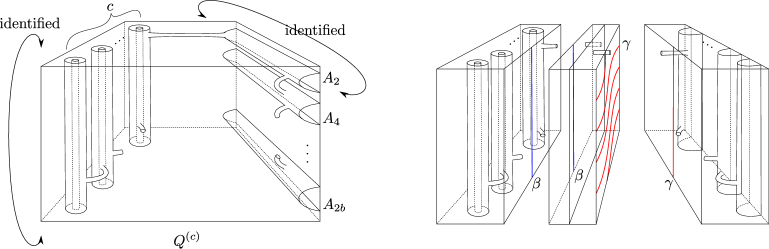
Figure 1. Relative Heegaard surfaces

We postpone the proof of Proposition 3.2 to the end of this section, as it will be an application of the next proposition which is of independent interest. We fix the following notation: glue $Q^{(b)}$ to $Q^{(c)}$ along a single boundary component and denote the slope of the Seifert fiber of $Q^{(b)}$ on the torus $Q^{(b)}\cap Q^{(c)}$ by $\beta$ and the slope of the Seifert fiber of $Q^{(c)}$ by $\gamma$. The manifold obtained is denoted $Q^{(b,c)}_{\beta,\gamma}$.

Proposition 3.4.

The genus of $Q^{(b,c)}_{\beta,\gamma}$ fulfils:

• If $\beta$ and $\gamma$ are complimentary slopes, then $g\big{(}Q^{(b,c)}_{\beta,\gamma}\big{)}=b+c$.

• If $\beta$ and $\gamma$ are not complimentary slopes, then $g\big{(}Q^{(b,c)}_{\beta,\gamma}\big{)}=b+c+1$.

We immediately obtain:

Corollary 3.5.

The surfaces in Figure 2 are minimal genus Heegaard splitting for $Q^{(b,c)}_{\beta,\gamma}$.

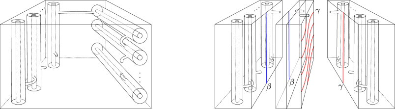
Figure 2. Heegaard surfaces for $Q^{(b,c)}_{\beta,\gamma}$

A surface in a Seifert fibered space is called vertical if it is everywhere tangent to the fibers and horizontal if it is everywhere transverse to the fibers. It is well known that given an essential surface in a Seifert fibered space we may assume it is vertical or horizontal; see for example, [7].

Proof of Proposition 3.4.

The surfaces in Figure 2 are Heegaard surfaces for $Q^{(b,c)}_{\beta,\gamma}$, showing the following, which we record here for future reference:

Remark 3.6.

When $\beta$ and $\gamma$ are complimentary, $g\big{(}Q^{(b,c)}_{\beta,\gamma}\big{)}\leq b+c$. When $\beta$ and $\gamma$ are not complimentary, $g\big{(}Q^{(b,c)}_{\beta,\gamma}\big{)}\leq b+c+1$.

Hence we only need to show that when $\beta$ and $\gamma$ are complimentary, $g\big{(}Q^{(b,c)}_{\beta,\gamma}\big{)}\geq b+c$ and when $\beta$ and $\gamma$ are not complimentary, $g\big{(}Q^{(b,c)}_{\beta,\gamma}\big{)}\geq b+c+1$.

If $\beta=\gamma$ then $Q^{(b,c)}_{\beta,\gamma}$ is a $b+c$ times punctured annulus cross $S^{1}$ and the result was proved by Schultens in [26]. For the remainder of the proof we assume that $\beta\neq\gamma$. Then $Q^{(b,c)}_{\beta,\gamma}$ is a graph manifold whose underlying graph consists of two vertices connected by a single edge. We apply Theorem 1.1 of Schultens [27] and refer the reader to that paper for notation and details. To conform to its noation, following [27], we decompose $Q^{(b,c)}_{\beta,\gamma}$ along two parallel copies of $Q^{(b)}\cap Q^{(c)}$ as $Q^{(b,c)}_{\beta,\gamma}=Q_{b}\cup M_{e}\cup Q_{c}$. $Q_{b}$ and $Q_{c}$ are called the vertex manifolds and $M_{e}$ is the edge manifold. Note that $Q_{b}\cong Q^{(b)}$, $M_{e}\cong T^{2}\times[0,1]$, and $Q_{c}\cong Q^{(c)}$.

Let $S$ be a minimal genus Heegaard splitting for $Q^{(b,c)}_{\beta,\gamma}$. In the following claim we analyze completely what happens when $g(S)=2$ or when $S$ is strongly irreducible:

Claim 3.7.

The following three conditions are equivalent:

1. $S$ is strongly irreducible.

2. The following conditions hold:

   • $\beta$ and $\gamma$ are complimentary.

   • $g(S)=2$.

   • $b=c=1$.

3. $g(S)=2$.

Proof of Claim 3.7.

(1) implies (2). Suppose that $S$ is strongly irreducible. By [27] we may assume that $S$ is standard. In particular, $S\cap Q_{b}$ (respectively $S\cap Q_{c}$) is either horizontal, pseudohorizontal, vertical, or pseudovertical. However, the first two cases are impossible as they require $S$ to meet every boundary component of $Q_{b}$ (respectively $Q_{c}$). Hence $S\cap Q_{b}$ and $S\cap Q_{c}$ consist of vertical or pseudovertical components. In particular, the intersection of $S$ with the torus $Q_{b}\cap M_{e}$ (respectively $Q_{c}\cap M_{e}$) is a Seifert fiber of $Q_{b}$ (respectively $Q_{c}$).

Assume first that $S\cap M_{e}$ is as in Case (1) of [27, Theorem 1.1], that is, $S\cap M_{e}$ is obtained from a collection incompressible annuli, say $\mathcal{A}$, by tubing along at most one boundary parallel arc (in [27], tubings are referred to as 1-surgary). Suppose that $\mathcal{A}$ consists of boundary parallel annuli. Since the tubing is performed, if at all, along a boundary parallel arc, we see that no component of $S\cap M_{e}$ connects the components of $\partial M_{e}$. This contradicts the fact that $S$ is connected and must meet both $Q_{b}$ and $Q_{c}$. Hence some component of $\mathcal{A}$ meets both components of $\partial M_{e}$, showing that $\beta=\gamma$, contradicting our assumption.

Hence Case (2) of [27, Theorem 1.1] holds, and $S\cap M_{e}$ consists of a single component that is obtained by tubing together two boundary parallel annuli, one at each boundary component of $M_{e}$; moreover, [27, Theorem 1.1] shows that these annuli define complementary slopes. See the left side of Figure 3. As argued above, the slopes defined by these annuli are $\beta$ and $\gamma$. This gives the first condition of (2).

Figure 3. Heegaard surface in $M_{e}$

On the right side of Figure 3 we see two surfaces. One is $S\cap M_{e}$, and in its center we marked the boundary of the obvious compressing disk. It is easy to see that the other surfce is isotopic to $S\cap M_{e}$. On it we marked the boundary of four disks, each shaped like $90^{o}$ sector. After gluing of opposite sides of the cube to obtained $M_{e}$, these sectors form a compressing disk on the opposite side of the obvious disk. This demonstrates that $S\cap M_{e}$ compresses into both sides. If $S\cap Q_{b}$ is pseudovertical then it compresses, and together with one of the compressing disks for $S\cap M_{e}$ we obtain a weak reduction, contradicting our assumption. Hence $S\cap Q_{b}$ consists of annuli; similarly, $S\cap Q_{c}$ consists of annuli. Hence $\chi(S)=\chi(S\cap M_{e})=-2$. The second condition of (2) follows.

Since $g(S)=2$, $\partial Q^{(b,c)}_{\beta,\gamma}$ consists of at most four tori. On the other hand, $\partial Q^{(b,c)}_{\beta,\gamma}$ consists of $b+c+2$ tori, for $b,c\geq 1$. Hence $b=c=1$, fulfilling the third and final condition of (2). This completes the proof that (1) implies (2).

It is trivial that (2) implies (3).

To see that (3) implies (1), assume that $S$ weakly reduces. Since $S$ is a minimal genus Heegaard surface and $g(S)=2$, an appropriate weak reduction yields an essential sphere, contradicting the fact that $Q^{(b,c)}_{\beta,\gamma}$ is irreducible.

This completes the proof of Claim 3.7. ∎

If $S$ is strongly irreducible, Proposition 3.4 follows from Claim 3.7. For the reminder of the proof we assume as we may that $S$ weakly reduces to a (possibly disconnected) essential surface, say $F$. By the construction of $Q^{(b,c)}_{\beta,\gamma}$ we see that every component of $F$ separates; hence by Proposition 2.3 we may assume that $F$ is connected. Recall that we assumed that $\beta\neq\gamma$. This clearly implies that we may suppose that (after isotopy if necessary) $F$ is disjoint from the torus $Q^{(b)}\cap Q^{(c)}$; without loss of generality we assume that $F\subset Q^{(b)}$.

We induct on $b+c$.

Base case: $b+c=2$. Note that in the base case $b=c=1$. It is easy to see that the only connected essential surface in $Q^{(1,1)}_{\beta,\gamma}$ is the torus $Q^{(b)}\cap Q^{(c)}$. Hence $F$ is isotopic to this surface and the weak reduction induces Heegaard splittings $\Sigma_{b}$ and $\Sigma_{c}$ on $Q^{(b)}$ and $Q^{(c)}$, respectively; note that both $Q^{(b)}$ and $Q^{(c)}$ are homeomorphic to $Q^{(1)}$. By Schultens [26], $g(Q^{(1)})=2$. by Lemma 2.2 amalgamation gives:

$$g(Q^{(1,1)}_{\beta,\gamma})=g(S)=g(\Sigma_{b})+g(\Sigma_{c})-g(F)\geq g(Q^{(1)})+g(Q^{(1)})-g(F)=2+2-1=3$$

By Remark 3.6, if $\beta$ and $\gamma$ are complimentary slopes then $g(Q^{(1,1)}_{\beta,\gamma})\leq 2$; hence $\beta$ and $\gamma$ are not complimentary slopes and together with Remark 3.6 the proposition follows in this case.

Inductive case: $b+c>2$. Assume, by induction, that the proposition holds for any integers $b^{\prime},c^{\prime}>0$, with $b^{\prime}+c^{\prime}<b+c$.

Case One: $F$ is isotopic to $Q^{(b)}\cap Q^{(c)}$. Then weak reduction induces Heegaard splittings on $Q^{(b)}$ and $Q^{(c)}$. Similar to the argument above (using that $g(Q^{(b)})=b+1$ and $g(Q^{(c)})=c+1$ by [26]) we have,

$$g(Q^{(b,c)}_{\beta,\gamma})\geq g(Q^{(b)})+g(Q^{(c)})-g(F)=b+c+1$$

As in the base case it follows from Remark 3.6 that $\beta$ and $\gamma$ are not complimentary slopes. Together with Remark 3.6, the proposition follows in this case.

Case Two: $F$ is not isotopic to $Q^{(b)}\cap Q^{(c)}$. Then $F$ is essential in $Q^{(b)}$ and is therefore isotopic to a vertical or horizontal surface. Since $F$ is closed and $\partial Q^{(b)}\neq\emptyset$, we have that $F$ cannot be horizontal. We conclude that $F$ is a vertical torus and decomposes $Q^{(b)}$ as $Q^{(b^{\prime})}$ (for some $b^{\prime}<b$) and a disk with $b-b^{\prime}+1$ holes cross $S^{1}$. By induction, the genus of $Q^{(b^{\prime},c)}_{\beta,\gamma}$ fulfills the conclusion of Proposition 3.4; by [26], the genus of disk with $b-b^{\prime}+1$ holes cross $S^{1}$ is $b-b^{\prime}+1$; similar to the argument above we get

$$g(Q^{(b,c)}_{\beta,\gamma})\geq g(Q^{(b^{\prime},c)}_{\beta,\gamma})+(b-b^{\prime}+1)-1=g(Q^{(b^{\prime},c)}_{\beta,\gamma})+b-b^{\prime}$$

Together with Remark 3.6, this completes the proof of Proposition 3.4. ∎

We are now ready to prove Proposition 3.2:

Proof of Proposition 3.2.

The surfaces in Figure 1 are relative Heegaard surfaces realizing the values given in Proposition 3.2. To complete the proof we only need to show that these surfaces realize the minimal relative genus.

Let $\Sigma$ be a minimal genus Heegaard surface for $Q^{(c)}$ relative to $\{A_{1},\dots,A_{2b}\}$. By tubing $\partial\Sigma$ along the annuli $A_{2i}$ and drilling a curve parallel to the core of $A_{2i}$ ($i=1,\dots,b$; recall Figure 1) we obtain a Heegaard surface for $Q^{(b,c)}_{\beta,\gamma}$ of genus $g(S)+b$. Thus $g(\Sigma)\geq g(Q^{(b,c)}_{\beta,\gamma})-b$. By Proposition 3.4, when $\beta$ and $\gamma$ are complimentary $g(Q^{(b,c)}_{\beta,\gamma})=b+c$ and when $\beta$ and $\gamma$ are not complimentary $g(Q^{(b,c)}_{\beta,\gamma})=b+c+1$. Thus we see that $g(\Sigma)\geq c$ (when the $\beta$ and $\gamma$ are complimentary) and $g(\Sigma)\geq c+1$ (otherwise).

This completes the proof of Proposition 3.2. ∎

Part II An upper bound on the growth rate of the tunnel number of knots

4. Haken Annuli

A primary tool in our study are Haken annuli. Haken annuli were first defined in [13], where only a single annulus was considered. We generalize the definition to a collection of annuli below. Note the similarity between a Haken annulus and a Haken sphere or Haken disk (by a Haken sphere we mean a sphere that meets a Heegaard surface in a single simple closed curve that is essential in the Heegaard surface, see [4] or [7, Chapter 2], and by a Haken disk we mean a disk that meets a Heegaard surface in a single simple closed curve that is essential in the Heegaard surface [3]).

Definition 4.1.

Let $C_{1}\cup_{\Sigma}C_{2}$ be a Heegaard splitting of a manifold $M$. A collection of essential annuli $\mathcal{A}\subset M$ are called Haken annuli for $C_{1}\cup_{\Sigma}C_{2}$ (or simply Haken annuli, when no confusion may arise) if for every annulus $A\in\mathcal{A}$ we have that $A\cap\Sigma$ consists of a single simple closed curve that is essential in $A$.

Remark 4.2.

For an integer $n\geq 2$, let $D(n)$ be a (disk with $n$ holes)$\times S^{1}$ and denote the components of $\partial D(n)$ by $T_{0},T_{1},\dots,T_{n}$. By the construction of minimal genus Heegaard splittings given in the proof of Proposition 2.14 of [13], we see that for each positive integers $p$ with $1\leq p\leq n$ there is a genus $n$ Heegaard surface of $(D(n);\cup_{i=0}^{p-1}T_{i},\cup_{i=p}^{n}T_{i})$ which admits a collection $\{A_{1},\dots,A_{p}\}$ of Haken annuli connecting $T_{i}$ to $T_{n}$ ($i=0,\dots,p-1$). By Schultens [26], we see that this is a minimal genus Heegaard splitting of $D(n)$. See Figure 4.

Figure 4. Heegaard surface in $D(n)$

In Propositions 3.5 and 3.6 of [13] we studied the behavior of Haken annuli under amalgamation. We generalise these propositions as Proposition 4.3 below. We first explain the construction that is used in Proposition 4.3. Let $C_{1}\cup_{\Sigma}C_{2}$ be a Heegaard splitting for a manifold $M$ that weakly reduces to a (possibly disconnected) essential surface $F$. Suppose that $M$ cut open along $F$ consists of two components, say $M^{(i)}$ $(i=1,2)$. We denote the image of $F$ in $M^{(i)}$ by $F^{(i)}$ and the Heegaard splitting induced on $M^{(i)}$ by $C_{1}^{(i)}\cup_{\Sigma^{(i)}}C_{2}^{(i)}$. Suppose that there are Haken annuli for $C_{1}^{(i)}\cup_{\Sigma^{(i)}}C_{2}^{(i)}$, say $\mathcal{A}^{(i)}$, satisfying the following two conditions:

• there exists a unique component of $\mathcal{A}^{(1)}$, say $A^{(1)}$, which intersects $F^{(1)}$ in a single simple closed curve, other components are disjoint from $F^{(1)}$, and

• each component of $\mathcal{A}^{(2)}$ intersects $F^{(2)}$ in a single simple closed curve isotopic in $F$ to $A^{(1)}\cap F^{(1)}$.

Then let $\widetilde{\mathcal{A}}^{(1)}$ be a collection of mutually disjoint annuli obtained from $\mathcal{A}^{(1)}$ by substituting $A^{(1)}$ with $|\mathcal{A}^{(2)}|$ parallel copies of $A^{(1)}$ whose boundaries are identified with $\mathcal{A}^{(2)}\cap F^{(2)}$. Finally let $\widetilde{\mathcal{A}}=\widetilde{\mathcal{A}}^{(1)}\cup\mathcal{A}^{(2)}$. Note that $\widetilde{\mathcal{A}}$ is a system of mutually disjoint annuli properly embedded in $M$. It is easy to adopt the proofs of Propositions 3.5 and 3.6 of [13] and obtain:

Proposition 4.3.

Let $M$, $C_{1}\cup_{\Sigma}C_{2}$, and $\widetilde{\mathcal{A}}$ be as above. Then the components of $\widetilde{\mathcal{A}}$ form Haken annuli for $C_{1}\cup_{\Sigma}C_{2}$.

5. Various decompositions of knot exteriors

In this section we compare two structures: Hopf-Haken annuli and $(h,b)$ decompositions. After defining the two we prove (Theorem 5.4) that they are equivalent.

Let $K$ be a knot in a 3-manifold $M$ and $h\geq 0$, $b\geq 1$ integers. We say that $K$ admits a $(h,b)$ decomposition (some authors use the term genus $h$, $b$ bridge position) if there exists a genus $h$ Heegaard splitting $C_{1}\cup_{\Sigma}C_{2}$ of $M$ such that $K\cap C_{i}$ is a collection of $b$ simultaneously boundary parallel arcs ($i=1,2$; note that in this paper we do not consider $(h,0)$ decomposition).

Let $K$ be a knot in a compact manifold $M$. Recall that $E(K)^{(c)}$ is obtained from $E(K)$ by removing $c$ curves that are simultaneously isotopic to meridians of $K$. The trace of the isotopy forms $c$ annuli which motivates the definition below (Definitions 5.1 and 5.2 generalize Definition 6.1 of [13]):

Definition 5.1 (a complete system of Hopf annuli).

Let $K\subset M$ be a knot in a compact manifold and $c>0$ an integer. Let $A_{1},\dots,A_{c}$ be annuli disjointly embedded in $E(K)^{(c)}$ so that for each $i$, one component of $\partial A_{i}$ is a meridian of $\partial N(K)$ and the other is a longitude of $T_{i}$ (recall $T_{1},\dots,T_{c}$ denote the components of $\partial E(K)^{(c)}\setminus\partial E(K)$). Then $\{A_{1},\dots,A_{c}\}$ is called a complete system of Hopf annuli. We emphasize that the complete system of Haken annuli for $E(K)^{(c)}$ is not unique up-to isotopy.

Definition 5.2 (a complete system of Hopf-Haken annuli).

Let $K\subset M$ be a knot in a compact manifold, $c>0$ an integer, $\Sigma$ a Heegaard surface for $E(K)^{(c)}$, and $\{A_{1},\dots,A_{c}\}$ a complete system of Hopf annuli. $\{A_{1},\dots,A_{c}\}$ is called a complete system of Hopf-Haken annuli for $\Sigma$ if for each $i$, $\Sigma\cap A_{i}$ is a single simple closed curve that is essential in $A_{i}$.

Definition 5.3 (Tubing bridge decomposition).

Let $K\subset M$ be a knot in a compact manifold, $\Sigma$ a Heegaard surface for $E(K)$, and $c>0$ an integer. Suppose that there exists a genus $h-c$ Heegaard surface for $M$ (say $S$) so that $K$ is $c$ bridge with respect to $S$, and the surface obtained by tubing $S$ along $c$ arcs of $K$ cut along $S$ on one side of $S$ is isotopic to $\Sigma$. Then we say that $\Sigma$ is obtained by tubing $S$ to one side (along $K$). See Figure 5.

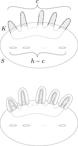
Figure 5. Tubing a $(h-c,c)$-decomposition

Theorem 5.4.

Let $M$ be a compact manifold and $K\subset M$ a knot and suppose the meridian of $K$ does not bound a disk in $E(K)$. Let $c,\ h$ be positive integers. Then the following two conditions are equivalent:

1. $K$ admits an $(h-c,c)$ decomposition.

2. $E(K)^{(c)}$ admits a genus $h$ Heegaard splitting that admits a complete system of Hopf-Haken annuli.

Proof.

$(1)\implies(2)$: Let $S\subset M$ be a surface defining a ($h-c$, $c$) decomposition. Then $S$ separates $M$ into two sides, say “above” and “below”; pick one, say above. Since the arcs of $K$ above $S$ form $c$ boundary parallel arcs (say $\alpha_{1},\dots,\alpha_{c}$), there are $c$ disjointly embedded disks above $K$ (say $D_{1},\dots,D_{c}$) so that $\partial D_{i}$ consists of two arcs, one $\alpha_{i}$ and the other along $S$ (for this proof, see Figure 5). Tubing $S$ $c$ times along $\alpha_{1},\dots,\alpha_{c}$ we obtain a Heegaard surface for $E(K)$ (say $\Sigma$). We may assume that the tubes are small enough, so that they intersect each $D_{i}$ in a single spanning arc. Denote the compression bodies obtained by cutting $E(K)$ along $\Sigma$ by $C_{1}$ and $C_{2}$ with $\partial N(K)\subset\partial_{-}C_{1}$. Then each $D_{i}\cap C_{2}$ is a meridional disk. Let $A_{1},\dots,A_{c}$ be $c$ meridional annuli properly embedded in $C_{1}$ near the maxima of $K$. Then $(\cup_{i}A_{i})\cap\partial N(K)$ consists of $c$ meridians, say $\alpha^{\prime}_{1},\dots,\alpha^{\prime}_{c}$. For each $i$, we isotope $\alpha^{\prime}_{i}$ along the annulus $A_{i}$ to the curve $A_{i}\cap\Sigma$ and then push it slightly into $C_{2}$, obtaining $c$ curves, say $\beta_{1},\dots,\beta_{c}$, parallel to meridians. Drilling $\cup_{i}\beta_{i}$ out of $E(K)$ gives $E(K)^{(c)}$. Using the disks $D_{i}\cap C_{2}$ it is easy to see that $\Sigma$ is a Heegaard surface for $E(K)^{(c)}$. Clearly, the trace of the isotopy from $\cup_{i=1}^{n}\alpha^{\prime}_{i}$ to $\cup_{i=1}^{n}\beta_{i}$ forms a complete system of Hopf annuli, and by construction every one of these annuli intersects $\Sigma$ in a single curve that is essential in the annulus. This completes the proof of $(1)\implies(2)$.

$(2)\implies(1)$: Assume that $E(K)^{(c)}$ admits a Heegaard surface of genus $h$, say $\Sigma$, with a complete system of Hopf-Haken annuli, say $\{A_{1},\dots,A_{c}\}$. Let $E(K)^{\prime}=\mbox{cl}(E(K)^{(c)}\setminus\cup_{i}N(A_{i}))$. Note that $E(K)^{\prime}$ is homeomorphic to $E(K)$. Let $S^{\prime}$ be the meridional surface $\Sigma\cap E(K)^{\prime}$. We may consider $M$ as obtained from $E(K)^{\prime}$ by meridional Dehn filling and $K$ as the core of the attached solid torus. By capping off $S^{\prime}$ we obtain a closed surface $S\subset M$. The following claim completes the proof of $(2)\implies(1)$:

Claim 5.5.

$S$ defines a ($h-c$, $c$) decomposition for $K$.

Proof of claim.

Recall that the components of $\partial E(K)^{(c)}\setminus\partial E(K)$ were denoted by $T_{1},\dots,T_{c}$, as in Definition 5.2, so that $A_{i}\cap T_{i}\neq\emptyset$ and $A_{i}\cap T_{j}=\emptyset$ (for $i\neq j$). Let $C_{1}$, $C_{2}$ be the compression bodies obtained from $E(K)^{(c)}$ by cutting along $\Sigma$, where $\partial N(K)\subset\partial_{-}C_{1}$. Since $\Sigma\cap A_{i}$ is a single simple closed curve which is essential in $A_{i}$ we have $T_{i}\subset\partial_{-}C_{2}$ ($i=1,\dots,c$). Denote the annulus $A_{j}\cap C_{i}$ by $A_{i,j}$ ($i=1,2$, $j=1,\dots,c$).

Let $C_{i}^{\prime}=C_{i}\cap E(K)^{\prime}$ $(i=1,2)$. It is clear that $S^{\prime}$ cuts $E(K)^{\prime}$ into $C_{1}^{\prime}$ and $C_{2}^{\prime}$. Since $A_{i}\cap\partial N(K)$ is a meridian of $K$, and by assumption the meridian of $K$ does not bound a disk in $E(K)$, we have that $A_{i,j}$ is incompressible in $C_{i}$. Hence a standard innermost disk, outermost arc argument shows that there is a system of meridian disks $\mathcal{D}_{i}$ of $C_{i}$ which cuts $C_{i}$ into $\partial_{-}C_{i}\times[0,1]$ such that $\mathcal{D}_{i}\cap(\cup A_{i,j})=\emptyset$.

Now we consider $C_{2}$ cut along $\cup A_{2,j}$. Since $\mathcal{D}_{2}\cap(\cup A_{2,j})=\emptyset$, there are components $T_{1}\times[0,1],\dots,T_{c}\times[0,1]$ of $C_{2}$ cut along $\mathcal{D}_{2}$, where $A_{2,j}\subset T_{j}\times[0,1]$ $(j=1,\dots,c)$. Here we note that $T_{j}\times[0,1]$ cut along $A_{2,j}$ is a solid torus in which the image of $T_{j}\times\{0\}$ is a longitudinal annulus (note that the image of $T_{j}\times\{0\}$ is exactly $T_{j}\cap C_{2}^{\prime}$). This shows that $\{T_{1}\cap C_{2}^{\prime},\dots,T_{c}\cap C_{2}^{\prime}\}$ is a primitive system of annuli in $C_{2}^{\prime}$, that is, there is a system of meridian disks $D_{2,1},\dots,D_{2,c}$ in $C_{2}^{\prime}$ such that $D_{2,j}\cap(T_{j}\cap C_{2}^{\prime})$ consists of a spanning arc of $T_{j}\cap C_{2}^{\prime}$, and $D_{2,j}\cap(T_{k}\cap C_{2}^{\prime})=\emptyset$ $(j\neq k)$. Let $C_{2}^{\prime\prime}$ be the manifold obtained from $C_{2}^{\prime}$ by adding $c$ 2-handles along $T_{1}\cap C_{2}^{\prime},\dots,T_{c}\cap C_{2}^{\prime}$. Since $\{T_{1}\cap C_{2}^{\prime},\dots,T_{c}\cap C_{2}^{\prime}\}$ is primitive, $C_{2}^{\prime\prime}$ is a genus $(h-c)$ compression body, and the union of the co-cores of the attached 2-handles, which can be regarded as $K\cap C_{2}^{\prime\prime}$, are simultaneously isotopic (through the disks $\cup D_{2,j})$ into $\partial_{+}C_{2}^{\prime\prime}$.

Analogously since $\mathcal{D}_{1}\cap(\cup A_{1,j})=\emptyset$, there are $c$ components of $C_{1}$ cut by $\mathcal{D}_{1}\cup(\cup A_{1,j})$ which are solid tori such that $\partial N(K)$ intersects each solid torus in a longitudinal annulus. Then the arguments in the last paragraph show that $K\cap C_{1}^{\prime\prime}$ consists of $c$ arcs which are simultaneously parallel to $S$.

These show that $S$ gives a $(h-c,c)$ decomposition for $K$, completing the proof of the claim. ∎

This completes the proof of Theorem 5.4. ∎

Corollary 5.6.

Let $K$ be a knot in a compact manifold $M$, and suppose that for some positive integers $h$ and $c$, $K$ admits a ($h-c$, $c$) decomposition. Then

$$g(E(K)^{(c)})\leq h$$

Proof.

This follows immediately from (1) $\implies$ (2) of Theorem 5.4. ∎

6. Existence of swallow follow tori and bounding $g(E(K_{1}\#\cdots\#K_{n})^{(c)})$ above

Definition 6.1 (Swallow Follow Torus).

Let $K\subset M$ be a knot and $c\geq 0$ an integer. An essential separating torus $T\subset E(K)^{(c)}$ is called a swallow follow torus if there exists an embedded annulus $A\subset E(K)^{(c)}$ with one component of $\partial A$ a meridian of $E(K)^{(c)}$ and the other an essential curve of $T$, so that $\mbox{int}(A)\cap T=\emptyset$.

In this definition (and throughout this paper) we allow $K$ to be the unknot in $S^{3}$, in which case $E(K)^{(c)}$ is homeomorphic to a disc with $c$ holes cross $S^{1}$, and it admits swallow follow tori whenever $c\geq 3$.

Given a swallow follow torus $T$ and an annulus $A$ as above, we can surger $T$ along $A$ to obtain a separating meridional annulus. It is easy to see that since $T$ is an essential torus, the annulus obtained is essential as well. Conversely, given an essential separating meridional annulus we can tube the annulus to itself along the boundary obtaining a swallow follow torus (this can be done in two distinct ways).

How does a swallow follow torus decompose a knot exterior? We first consider the case $c=0$. Let $K=K_{1}\#K_{2}$ be a composite knot (here we are not assuming that $K_{1}$ or $K_{2}$ is prime). Let $\mathcal{A}$ be a decomposing annulus corresponding to the decomposition of $K$ as $K_{1}\#K_{2}$. Thus $E(K)=E(K_{1})\cup_{\mathcal{A}}E(K_{2})$. Tubing $\mathcal{A}$ along the boundary (say into $E(K_{2})$) we obtain a swallow follow torus, say $T$. Clearly, one component of $E(K)$ cut open along $T$ is homeomorphic to $E(K_{2})$. The other component is homeomorphic to $E(K_{1})$ with two meridional annuli identified, and hence homeomorphic to $E(K_{1})^{(1)}$. Thus we see that a swallow follow torus $T\subset E(K)$ decomposes $E(K)$ as $E(K_{1})^{(1)}\cup_{T}E(K_{2})$. More generally, given $K,\ K_{1},\ K_{2}$ as above and integers $c,\ c_{1},\ c_{2}\geq 0$ with $c_{1}+c_{2}=c$, let $\mathcal{A}$ be a decomposing annulus for $E(K)^{(c)}$, so that $E(K)^{(c)}=E(K_{1})^{(c_{1})}\cup_{\mathcal{A}}E(K_{2})^{(c_{2})}$. The swallow follow torus obtained by tubing $\mathcal{A}$ into $E(K_{2})^{(c_{2})}$ decomposes $E(K)^{(c)}$ as $E(K_{1})^{(c_{1}+1)}\cup_{T}E(K_{2})^{(c_{2})}$. Since the components of $E(K)^{(c)}$ cut open along a swallow follow torus are themselves of the form $E(K_{1})^{(c_{1}+1)}$ and $E(K_{2})^{(c_{2})}$, we may now extend Definition 6.1 inductively:

Definition 6.2 (Swallow Follow Tori).

Let $K$ and $c$ be as in the previous paragraph. Let $T_{1},\dots,T_{r}$ (for some $r$) be disjointly embedded tori in $E(K)^{(c)}$. Then $T_{1},\dots,T_{r}$ are called swallow follow tori if the following two conditions hold, perhaps after reordering the indices:

1. $T_{1}$ is a swallow follow torus for $E(K)^{(c)}$.

2. For each $i\geq 2$, $T_{i}$ is a swallow follow torus for some component of $E(K)^{(c)}$ cut open along $\cup_{j=1}^{i-1}T_{j}$.

We are now ready to state and prove:

Proposition 6.3 (Existence of Swallow Follow Tori).

For $i=1,\dots,n$, let $K_{i}$ be a (not necessarily prime) knot in a compact manifold and let $c\geq 0$ be an integer. Suppose that $E(K_{i})\not\cong T^{2}\times[0,1]$ and $\partial N(K_{i})$ is incompressible in $E(K_{i})$.

Then given any integers $c_{1},\dots,c_{n}\geq 0$ whose sum is $c+n-1$, there exist $n-1$ swallow follow tori, denoted $\mathcal{T}$, that decompose $E(\#_{i=1}^{n}K_{i})^{(c)}$ as:

$$E(\#_{i=1}^{n}K_{i})^{(c)}=\cup_{\mathcal{T}}E(K_{i})^{(c_{i})}$$

Proof.

We use the notation as in the statement of the proposition and induct on $n$. If $n=1$ there is nothing to prove. We assume as we may that $n>1$.

We first claim that for some $i$ we have that $c_{i}\leq c$. Assume, for a contradiction, that $c_{i}>c$ for every $1\leq i\leq n$. Since $c_{i}$ and $c$ are integers, $c_{i}\geq c+1$. Then we have:

$$c+n-1=\sum_{i=1}^{n}c_{i}\geq n(c+1)=nc+n$$

Moving all term to the right we get that

$$0\geq(n-1)c+1$$

which is absurd, since $n\geq 1$ and $c\geq 0$. By reordering the indices if necessary we may assume that $c_{n}\leq c$.

Let $A$ be an annulus in $E(\#_{i=1}^{n}K_{i})$ so that the components of $E(\#_{i=1}^{n}K_{i})$ cut open along $A$ are identified with $E(K_{1}\#\cdots\#K_{n-1})$ and $E(K_{n})$. Since the tori $\partial N(K_{i})$ are incompressible, $A$ is essential in $E(\#_{i=1}^{n}K_{i})$. Recall that $E(\#_{i=1}^{n}K_{i})^{(c)}$ is obtained from $E(\#_{i=1}^{n}K_{i})$ by drilling $c$ curves that are parallel to the meridian; since $c_{n}\leq c$ we may choose the curves so that exactly $c_{n}$ components are contained in $E(K_{n})$. After drilling, the components of $E(\#_{i=1}^{n}K)^{(c)}$ cut open along $A$ are identified with $E(K_{1}\#\cdots\#K_{n-1})^{(c-c_{n})}$ and $E(K_{n})^{(c_{n})}$. Let $T$ be the torus obtained by tubing $A$ into $E(K)^{(c_{n})}$; clearly the components of $E(\#_{i=1}^{n}K)^{(c)}$ cut open along $T$ are identified with $E(K_{1}\#\cdots\#K_{n-1})^{(c-c_{n}+1)}$ and $E(K_{n})^{(c_{n})}$. Since $A$ is essential and $E(K_{i})\not\cong T^{2}\times[0,1]$, we have the $T$ is essential in $E(\#_{i=1}^{n}K_{i})^{(c)}$. By construction, there is an essential curve on $T$ that cobounds an annulus with a meridian of $E(\#_{i=1}^{n}K_{i})^{(c)}$ and we conclude that $T$ is a swallow follow torus.

We induct on $K_{1},\dots,K_{n}$. Let $c^{\prime}=c-c_{n}+1$. Then we have

$$\sum_{i=1}^{n-1}c_{i}=\sum_{i=1}^{n}c_{i}-c_{n}=c+n-1-c_{n}=(c-c_{n}+1)+n-2=c^{\prime}+(n-1)-1$$

By induction, $E(K_{1}\#\cdots\#K_{n-1})^{(c^{\prime})}$ admits $n-2$ swallow follow tori, which we will denote by $\mathcal{T}^{\prime}$, so that $\mathcal{T}^{\prime}$ decomposes $E(K_{1}\#\cdots\#K_{n-1})^{(c^{\prime})}=E(K_{1}\#\cdots\#K_{n-1})^{(c-c_{n}+1)}$ as

$$\cup_{\mathcal{T}^{\prime}}E(K_{i})^{(c_{i})}$$

It follows that $\mathcal{T}=T\cup\mathcal{T}^{\prime}$ are swallow follow tori for $E(K)^{(c)}$, and the components of $E(K)^{(c)}$ cut open along $\mathcal{T}$ are homeomorphic to $E(K_{1})^{(c_{1})},\dots,E(K_{n})^{(c_{n})}$.

∎

By Proposition 6.3 and repeated application of Lemma 2.2 we obtain the following.

Corollary 6.4.

With notation as in the statement of Proposition 6.3 (and in particular for any integer $c\geq 0$, any integers $c_{1},\dots,c_{n}$ whose sum is $c+n-1$), we get:

$$g(E(K)^{(c)})\leq\Sigma_{i=1}^{n}g(E(K_{i})^{(c_{i})})-(n-1)$$

7. An upper bound for the growth rate

Using the results in the previous sections we can easily bound the growth rate:

Proposition 7.1.

Let $K$ be an admissible knot in a closed manifold $M$. Let $g=g(E(K))-g(M)$ and the bridge indices $\{b_{1}^{*},\dots,b_{g}^{*}\}$ be as in Notation 1.1 in the introduction.

Then

$$\mbox{gr}_{t}(K)\leq\min_{i=1,\dots,g}\bigg{\{}1-\frac{i}{b_{i}^{*}}\bigg{\}}$$

Proof.

Fix $1\leq i\leq g$ and a positive integer $n$. Let $k_{i}>0$ and $0\leq r<b_{i}^{*}$ be the quotient and remainder when deviding $(n-1)$ by $b_{i}^{*}$; that is:

$$k_{i}b^{*}_{i}+r=n-1$$

Consider the non-negative integers $b_{i}^{*},\dots,b^{*}_{i},r,0,\dots,0$ (where $b_{i}^{*}$ appears $k_{i}$ times and the symbol $0$ appears $n-(k_{i}+1)$ times). Applying Corollary 6.4 to $E(nK)^{(0)}$ we get (recall that $E(nK)^{(0)}=E(nK)$):

$$g(E(nK))\leq k_{i}g(E(K)^{(b_{i}^{*})})+g(E(K)^{(r)})+(n-(k_{i}+1))g(E(K))-(n-1)$$

By definition of $b_{i}^{*}$, $K$ admits a ($g(E(K))-i,b_{i}^{*}$) decomposition. Applying Corollary 5.6 with $h-c=g(E(K))-i$ and $c=b_{i}^{*}$ gives

$$g(E(K)^{(b_{i}^{*})})\leq g(E(K))-i+b_{i}^{*}$$

Thus we get:

$$g(E(nK)) \leq k_{i}(g(E(K))-i+b_{i}^{*})+g(E(K)^{(r)})+(n-(k_{i}+1))g(E(K))-(n-1)$$

$$= (n-1)g(E(K))+g(E(K)^{(r)})-k_{i}i+(k_{i}b_{i}^{*}-(n-1))$$

$$= (n-1)g(E(K))+g(E(K)^{(r)})-k_{i}i-r$$

By denoting the $n$-th element of the sequence in the definition of the growth rate by $S_{n}$, we get:

$$S_{n} = \frac{g(E(nK))-ng(E(K))+(n-1)}{n-1}$$

$$\leq \frac{1}{n-1}[(n-1)g(E(K))+g(E(K)^{(r)})-k_{i}i-r-ng(E(K))+(n-1)]$$

$$= \frac{1}{n-1}[g(E(K)^{(r)})-g(E(K))-r-k_{i}i+(n-1)]$$

$$= \frac{g(E(K)^{(r)})-g(E(K))-r}{n-1}+1-\frac{k_{i}i}{k_{i}b_{i}^{*}+r}$$

In the last equality we used $k_{i}b^{*}_{i}+r=n-1$. Recall that $E(K)^{(r)}$ is obtained by drilling $r$ curve parallel to $\partial E(K)$ out of $E(K)$. Therefore by [22], $g(E(K)^{(r)})\leq g(E(K))+r$. Hence the first summand above is non-positive, and we may remove that term. Furthermore since $r<b_{i}^{*}$, $k_{i}b_{i}^{*}+r<(k_{i}+1)b_{i}^{*}$, which implies

(1) $$S_{n}<1-\frac{i}{b_{i}^{*}}\frac{k_{i}}{k_{i}+1}$$

Since $\lim_{n\to\infty}k_{i}=\infty$ we have:

$$\mbox{gr}_{t}(K)=\limsup_{n\to\infty}S_{n}\leq\lim_{k_{i}\to\infty}\biggl{(}1-\frac{i}{b_{i}^{*}}\frac{k_{i}}{k_{i}+1}\biggr{)}=1-\frac{i}{b_{i}^{*}}$$

As $i$ was arbitrary, we get that

$$\mbox{gr}_{t}(K)\leq\min_{i=1,\dots,g}\bigg{\{}1-\frac{i}{b_{i}^{*}}\bigg{\}}$$

This completes the proof of Proposition 7.1. ∎

Part III The growth rate of m-small knots

This part is devoted to calculating the growth rate of m-small knots, completing the proof of Theorem 1.2. Section 8 contains the main technical result of this paper, the Strong Hopf Haken Annulus Theorem (Theorem 1.7). This result guarantees the existence of Hopf–Haken annuli, and complements Sections 4 and  5. In Section 9 we prove existence of “special” swallow follow tori; this section complements Section 6. Finally, in Section 10 we calculate the growth rate of m-small knots by finding a lower bound that equals exactly the upper bound found in Section 7.

8. The Strong Hopf-Haken Annulus Theorem

Given a knot $K$ in a compact manifold $M$ and an integer $c>0$; recall that the exterior of $K$ is denoted by $E(K)$, the manifold obtained by drilling out $c$ curves simultaneously parallel to the meridian of $E(K)$ is denoted by $E(K)^{(c)}$, and the components of $\partial E(K)^{(c)}\setminus\partial E(K)$ are denoted by $T_{1},\dots,T_{c}$. Recall also the definitions of Haken annuli for a given Heegaard splitting (4.1), a complete system of Hopf annuli (5.1), and a complete system of Hopf-Haken annuli for a given Heegaard splitting (5.2).

In this section we prove the Strong Hopf Haken Annulus Theorem (Theorem 1.7), stated in the introduction. Before proving Theorem 1.7 we prove three of its main corollaries:

Corollary 8.1.

Suppose that the assumptions of Theorem 1.7 are satisfied with $F_{1}=F_{2}=\emptyset$ and in addition, for each $i$, $E(K_{i})$ does not admit an essential meridional surface $S$ with $\chi(S)\geq 6-2g(E(K)^{(c)})$. Let $h\geq 0$ be an integer. Then $K$ admits an $(h-c,c)$ decomposition if and only if $g(E(K)^{(c)})\leq h$.

Proof of Corollary 8.1.

Assume first that $K$ admits an $(h-c,c)$ decomposition. Then by Corollary 5.6, we have $g(E(K)^{(c)})\leq h$. Note that this direction holds in general and does not require the assumption about meridional surfaces.

Next assume that $g(E(K)^{(c)})\leq h$ and let $\Sigma\subset E(K)^{(c)}$ be a genus $h$ Heegaard surface. By the assumptions of the corollary, Conclusion (2) of Theorem 1.7 does not hold. Hence by that theorem $E(K)^{(c)}$ admits a genus $h$ Heegaard surface that admits a complete system of Hopf-Haken annuli. By $(2)\Rightarrow(1)$ of Theorem 5.4, $K$ admits an $(h-c,c)$ decomposition. ∎

Corollary 8.2.

We use the notation of Theorem 1.7. Suppose that the assumptions of Theorem 1.7 hold and in addition, that each $K_{i}$ is m-small. Then for any $c$ and any choice of $F_{1}$ and $F_{2}$, there is a minimal genus Heegaard splitting of $(E(\#_{i=1}^{n}K_{i})^{(c)};F_{1},F_{2})$ that admits a complete system of Hopf-Haken annuli.

Proof of Corollary 8.2.

This follows immediately from Theorem 1.7. ∎

Next we prove Corollary 1.8 which was stated in the introduction:

Proof of Corollary 1.8.

We fix the notation in the statement of the corollary. First we show that for any knot $K$ (not necessarily the connected sum of m-small knots) if $c\geq b_{g}^{*}$, then the inequality $g(E(K)^{(c)})\leq c$ holds: by definition of $b_{g}^{*}$, $K$ admits a $(0,b_{g}^{*})$ decomposition (recall that $K\subset S^{3}$ and hence $b_{g}^{*}$ is the bridge index of $K$ with respect to $S^{2}$). Thus for $c\geq b_{g}^{*}$, $K$ admits a $(0,c)$ decomposition. By viewing this as a $(c-c,c)$ decomposition, Corollary 5.6 implies that $g(E(K)^{(c)})\leq c$.

Next we note that the inequality $g(E(K)^{(c)})\geq c$ holds for $K$ that is a connected sum of m-small knots, and any $c\geq 0$: by Corollary 8.2, $E(K)^{(c)}$ admits a minimal genus Heegaard surface (say $\Sigma$) admitting a complete system of Hopf–Haken annuli. Hence the $c$ tori, $T_{1},\dots,T_{c}$, are on the same side of $\Sigma$, which implies $g(\Sigma)\geq c$; hence $g(E(K)^{(c)})=g(\Sigma)\geq c$.

∎

Proof of Theorem 1.7.

We first fix the notation that will be used in the proof (in addition to the notation in the statement of the theorem). Let $K$ denote $\#_{i=1}^{n}K_{i}$. For $c>0$, $E(K)^{(c)}$ admits an essential torus $T$ that decomposes $E(K)^{(c)}$ as:

$$E(K)^{(c)}=X\cup_{T}Q^{(c)},$$

where $X\cong E(K)$ and $Q^{(c)}\cong\mbox{ (annulus with }c\mbox{ holes)}\times S^{1}$. Note that $Q^{(c)}$ fibers over $S^{1}$ in a unique way, and the fibers in $T$ are meridian curves in $X\cap Q^{(c)}$. Since $Q^{(c)}$ is Seifert fibered it is contained in a unique component $J$ of the characteristic submanifold [7], [8], [9]. Since $\partial N(K_{i})$ is incompressible in $E(K_{i})$, using Miyazaki’s result [17] it was shown in [13, Claim 1] that $K$ admits a unique prime decomposition. Therefore the number of prime factors of $K$ is well-defined. We suppose as we may that each knot $K_{i}$ is prime; consequently, the integer $n$ appearing in the statement of the theorem is the number of prime factors of $K$.

Figure 6.

The structure of the Proof. The proof is an induction on $(n,c)$ ordered lexicographically. We begin with two preliminary special cases. In Case One we consider strongly irreducible Heegaard splittings. In Case Two we consider weakly reducible Heegaard splittings so that no component of the essential surface obtained by untelescoping is contained in $J$. In both cases we prove the theorem directly and without reference to the complexity $(n,c)$. We then proceed to the inductive step assuming the theorem for $(n^{\prime},c^{\prime})<(n,c)$ in the lexicographic order. By Cases One and Two we may assume that a minimal genus Heegaard surface for $E(K)^{(c)}$ is weakly reducible and some component of the essential surface obtained by untelescoping it is contained in $J$; this component allows us to induct.

Case One. $(E(K)^{(c)};F_{1},F_{2})$ admits a strongly irreducible minimal genus Heegaard splitting. Let $C_{1}\cup_{\Sigma}C_{2}$ be a minimal genus strongly irreducible Heegaard splitting of $(E(K)^{(c)};F_{1},F_{2})$. The Swallow Follow Torus Theorem [13, Theorem 4.1] implies that f $n>1$, either $\Sigma$ weakly reduces to a swallow follow torus (which contradicts the assumption of Case One) or Conclusion 2 of Theorem 1.7 holds. We assume as we may that $n=1$ in the remainder of the proof of Case One.

Recall the notation $E(K)^{(c)}=X\cup_{T}Q^{(c)}$. Since $T\subset E(K)^{(c)}$ is essential and $\Sigma\subset E(K)^{(c)}$ is strongly irreducible, we may isotope $\Sigma$ so that $\Sigma\cap T$ is transverse and every curve of $\Sigma\cap T$ is essential in $T$. Minimize $|\Sigma\cap T|$ subject to this constraint. If $\Sigma\cap T=\emptyset$ then $T$ is contained in a compression body $C_{1}$ or $C_{2}$, and hence $T$ is parallel to a component of $\partial_{-}C_{1}$ or $\partial_{-}C_{2}$. But then $T$ is parallel to a component of $\partial E(K)^{(c)}$, a contradiction. Thus $\Sigma\cap T\neq\emptyset$.

Let $F$ be a component of $\Sigma$ cut open along $T$. Minimality of $|\Sigma\cap T|$ implies that $F$ is not boundary parallel. Then $\partial F\subset T$; since $T$ is a torus, boundary compression of $F$ implies compression into the same side; this will be used extensively below. A surface in a Seifert fibered manifold is called vertical if it is everywhere tangent to the fibers and horizontal if it is everywhere transverse to the fibers (see, for example, [7] for a discussion). We first reduce Theorem 1.7 as follows:

Assertion 1.

One of the following holds:

1. $\Sigma\cap X$ is connected and compresses into both sides, and $\Sigma\cap Q^{(c)}$ is a collection of essential vertical annuli.

2. Theorem 1.7 holds.

Proof.

A standard argument shows that one component of $\Sigma$ cut open along $T$ compresses into both sides (in $X$ or $Q^{(c)}$) and all other components are essential (in $X$ or $Q^{(c)}$); for the convenience of the reader we sketch it here: let $D_{1}$ be a compressing disk for $C_{1}$. After minimizing $|D_{1}\cap T|$ either $D_{1}\cap T=\emptyset$ (and hence some component of $\Sigma$ cut open along $T$ compresses into $C_{1}$) or an outermost disk of $D_{1}$ provides a boundary compression for some component of $\Sigma$ cut open along $T$; since boundary compression implies compression into the same side, we see that in this case too some component of $\Sigma$ cut open along $T$ compresses into $C_{1}$. Similarly, some component of $\Sigma$ cut open along $T$ compresses into $C_{2}$. Strong irreducibility of $\Sigma$ implies that the same component compresses into both sides and all other components are incompressible and boundary incompressible. Minimality of $|\Sigma\cap T|$ implies that no component is boundary parallel, and hence the incompressible and boundary incompressible components are essential.

The proof of Assertion 1 breaks up into three subcases:

Subcase 1: no component of $\Sigma\cap X$ is essential. Then $\Sigma\cap X$ is connected and compresses into both sides, and therefore $\Sigma\cap Q^{(c)}$ consists of essential surfaces. Since $Q^{(c)}$ is Seifert fibered, every component of $\Sigma\cap Q^{(c)}$ is either horizontal of vertical (see, for example, [7, VI.34]). Any horizontal surface in $Q^{(c)}$ must meet every component of $\partial Q^{(c)}$; by construction $\Sigma\cap\partial N(K)=\emptyset$; thus every component of $\Sigma\cap Q^{(c)}$ is vertical (we will use this argument below without reference). This gives Conclusion (1) of the assertion.

Subcase 2.a: some component of $\Sigma\cap X$ is essential and some component of $\Sigma\cap Q^{(c)}$ is essential. Let $F$ denote an essential component of $\Sigma\cap X$. Since $T$ is incompressible and the components of $\Sigma\cap T$ are essential in $T$, no component of $\Sigma$ cut open along $T$ is a disk; hence $\chi(F)\geq\chi(\Sigma)$. Let $S$ denote an essential component of $\Sigma\cap Q^{(c)}$. Then $S$ is a vertical annulus. In particular, $S\cap T$ consists of fibers in the Seifert fiberation of $Q^{(c)}$. By construction, the fibers on $T$ are meridians of $X$. We see that $F$ is meridional, giving Conclusion (2) of Theorem 1.7.

Subcase 2.b: some component of $\Sigma\cap X$ is essential and no component of $\Sigma\cap Q^{(c)}$ is essential. As above let $F$ be an essential component of $\Sigma\cap X$. By assumption, no component of $\Sigma\cap Q^{(c)}$ is essential. Hence $\Sigma\cap Q^{(c)}$ is connected and compresses into both sides. Let $\Delta_{1}$ be a maximal collection of compressing disks for $\Sigma\cap Q^{(c)}$ into $Q^{(c)}\cap C_{1}$ and $S_{1}$ the surface obtained by compressing $S$ along $\Delta_{1}$. Since $\Delta_{1}\neq\emptyset$, maximality of $\Delta_{1}$ and the no nesting lemma [23] imply that $S_{1}$ is incompressible. Suppose first that some non-closed component of $S_{1}$, say $S_{1}^{\prime}$, is not boundary parallel (this is similar to Subcase 2.a). Then $S_{1}^{\prime}$ is an essential and hence vertical annulus and we see that $F$ is meridional, giving Conclusion (2) of Theorem 1.7 and the assertion follows. We assume from now on that $S_{1}$ consists of boundary parallel annuli and, perhaps, closed boundary parallel surfaces and ball-bounding spheres. Furthermore, we see that:

1. No two closed components of $S_{1}$ are parallel to the same component of $\partial Q^{(c)}$: this follows from connectivity of $\Sigma\cap Q^{(c)}$ and strong irreducibility of $\Sigma$.

2. No two boundary parallel annuli of $S_{1}$ are nested: otherwise, it follows from connectivity of $\Sigma\cap Q^{(c)}$ and strong irreducibility of $\Sigma$ that $\Sigma$ can be isotoped out of $Q^{(c)}$; for more details see [11, Page 249].

We assume as we may that the analogous conditions hold after compressing $\Sigma\cap Q^{(c)}$ into $Q^{(c)}\cap C_{2}$. Hence $\Sigma\cap Q^{(c)}$ is a Haagaard surface for $Q^{(c)}$ relative to the annuli $\{C_{1}\cap T,C_{2}\cap T\}$ (relative Heegaard surfaces were defined in 3.1). We may replace $\Sigma\cap Q^{(c)}$ with the minimal genus relative Heegaard surface for $Q^{(c)}$ relative to $\{C_{1}\cap T$, $C_{2}\cap T\}$ given in Corollary 3.3. By pasting this surface to $\Sigma\cap X$ we obtain a closed surface, say $\Sigma^{\prime}$, fulfilling for following conditions:

1. $\Sigma^{\prime}$ is a Heegaard surface for $E(K)^{(c)}$: the components of $X$ cut open along $\Sigma\cap X$ are the same as the components of $C_{1}$ and $C_{2}$ cut open along $\{C_{1}\cap T,C_{2}\cap T\}$. Since $T$ is essential, the annuli $C_{i}\cap T$ are incompressible in $C_{i}$. It is well known that cutting a compression body along incompressible surfaces yields compression bodies; we conclude that the components of $X$ cut open along $\Sigma\cap X$ are compression bodies. By definition of relative Heegaard surface, the annuli of $\{C_{1}\cap T,C_{2}\cap T\}$ are primitive in the compression bodies obtained by cutting $Q^{(c)}$ open along any relative Heegaard surface; it follows that $E(K)^{(c)}$ cut open alone $\Sigma^{\prime}$ consists of two compression bodies.

2. $\Sigma^{\prime}$ is a Heegaard surface for $(E(K)^{(c)};F_{1},F_{2})$: in addition to (1) above, we need to show that $\Sigma^{\prime}$ respects the same partition of $\partial E(K)^{(c)}\setminus(\partial N(K),T_{1},\dots,T_{c})$ as $\Sigma$. This follows immediately from the facts that the changes we made are contained in $Q^{(c)}$, every component of $F_{1}$ is contained in $C_{1}\cap X$, and every component of $F_{2}$ is contained in $C_{2}\cap X$. Note that (1) and (2) hold for any relative Heegaard surface for $Q^{(c)}$ relative to $\{C_{1}\cap T$, $C_{2}\cap T\}$.

3. $g(\Sigma^{\prime})=g(\Sigma)$: minimality of the genus of the relative Heegaard splitting used implies that $g(\Sigma^{\prime})\leq g(\Sigma)$; as $\Sigma$ was a minimal genus Heegaard surface for $(E(K)^{(c)};F_{1},F_{2})$, $g(\Sigma^{\prime})=g(\Sigma)$. Note that (3) hold for any minimal genus relative Heegaard surface for $Q^{(c)}$ relative to $\{C_{1}\cap T$, $C_{2}\cap T\}$.

4. $\Sigma^{\prime}$ admits a completes system of Hopf-Haken annuli: By Figure 1 we see directly $\Sigma^{\prime}$ admits a complete system of Hopf Haken annuli.

Remark 8.3.

As noted, in the construction above (3) holds for any minimal genus relative Heegaard surface. This is quite different in (4), when considering Hopf-Haken annuli: it is not hard to construct relative Heegaard surfaces that result in a minimal genus Heegaard surface for $(E(K)^{(c)};F_{1},F_{2})$ so that all the tori $T_{1}.\dots,T_{c}$ are in the compression body containing $\partial N(K)$, and hence cannot admit even one Hopf-Haken annulus. This shows that in the course of the proof of Theorem 1.7 the given Heegaard surface must be replaced.

The Heegaard surface $\Sigma^{\prime}$ fulfils the conditions of Conclusion (1) of Theorem 1.7. This completes that proof of Assertion 1. ∎

Before proceeding we fix the following notation and conventions: denote $\Sigma\cap X$ by $\Sigma_{X}$. By Assertion 1 we may assume that $\Sigma_{X}$ is connected and compresses into both sides and every component of $\Sigma\cap Q^{(c)}$ is an essential vertical annulus. Note that $X$ cut open along $\Sigma_{X}$ consists of exactly two components, denoted by $C_{i,X}$, where $C_{i,X}=C_{i}\cap X$ ($i=1,2$). Denote the collection of annuli $T\cap C_{i,X}$ by $\mathcal{A}_{i}$, and the annuli in $\mathcal{A}_{i}$ by $A_{i,1},\dots,A_{i,b}$, where $b$ denotes the number of annuli in $\mathcal{A}_{i}$. We assume from now on that Conclusion (2) of Theorem 1.7 does not hold.

Assertion 2.

The number $b$ fulfils $c\leq b\leq g(\Sigma)$.

Proof.

Assume for a contradiction that $b<c$. Since $\Sigma\cap Q^{(c)}$ consists of $b$ annuli, $Q^{(c)}$ cut open along $\Sigma\cap Q^{(c)}$ consists of $b+1<c+1$ components. Hence some component of $Q^{(c)}$ cut open along $\Sigma\cap Q^{(c)}$ contains two of the components of $\partial Q^{(c)}\setminus T$. Hence there is a vatical annulus connecting these components which is disjoint from $\Sigma$. Since this annulus is disjoint from $\Sigma$ it is contained in a compression body $C_{i}$ and connects two components of $\partial_{-}C_{i}$, which is impossible.

Since $\Sigma_{X}$ is obtained by removing the $b$ annuli $\Sigma\cap Q^{(c)}$ and is connected, $b\leq g(\Sigma)$.

This completes the proof of Assertion 2. ∎

Assertion 3.

The surface $\Sigma_{X}$ defines a $(g(\Sigma)-b,b)$ decomposition of $K$.

Proof.

For $i=1,2$, let $\Delta_{i}$ be a maximal collection of compressing disks for $\Sigma_{X}$ into $C_{i,X}$; by assumption, $\Delta_{i}\neq\emptyset$. Let $S_{i}$ be the surface obtained by compressing $\Sigma_{X}$ along $\Delta_{i}$. By maximality and the no nesting lemma [23] $S_{i}$ is incompressible. Since the components of $\Sigma\cap Q^{(c)}$ are vertical annuli, the boundary components of $S_{i}$ are meridians. Hence, if some non-closed component of $S_{i}$ is essential, we obtain Conclusion (2) of Theorem 1.7, contradicting our assumption. Thus $S_{i}$ consists of boundary parallel annuli and, perhaps, closed boundary parallel surfaces and ball-bounding spheres. As above, strong irreducibility of $\Sigma$ and connectivity of $\Sigma_{X}$ imply that these annuli are not nested. We see that $C_{i,X}$ is a compression body and $T\cap C_{i,X}$ consists of $b$ mutually primitive annuli. In fact, we see that $\Sigma_{X}$ is a relative Heegaard surface. By the argument of Claim 5.5, on Page 5.5, $\Sigma_{X}$ gives a $(g(\Sigma)-b,b)$ decomposition. ∎

By Assertion 3 and Theorem 5.4, $E(K)^{(b)}$ admits a genus $g(\Sigma)$ Heegaard surface admitting a complete system of Hopf-Haken annuli, say $\Sigma^{\prime}$. By Assertion 2, $c\leq b$. Hence $E(K)^{(c)}$ is obtained from $E(K)^{(b)}$ by filling the tori $T_{c+1},\dots,T_{b}$. Clearly, $\Sigma^{\prime}$ is a Heegaard surface for $E(K)^{(c)}$, admitting a complete system of Hopf-Haken annuli. This completes the proof of Theorem 1.7 in Case One.

Before proceeding to Case Two we introduce notation that will be used in that case. Recall that since $Q^{(c)}$ is Seifert fibered, it is contained in a component of the characteristic submanifold of $E(K)^{(c)}$ denoted by $J$. Since $X\cong E(K)$ and $K=\#_{i=1}^{n}K_{i}$, $X$ admits $n-1$ decomposing annuli which we will denote by $A_{1},\dots,A_{n-1}$ ($A_{1},\dots,A_{n-1}$ are not uniquely defined). The components of $X$ cut open along $\cup_{i=1}^{n-1}A_{i}$ are homeomorphic to $E(K_{1}),\dots,E(K_{n})$. Let $V=Q^{(c)}\cup N(A_{1})\cup\cdots\cup N(A_{n-1})$. Then $V$ is Seifert fibered and contains $Q^{(c)}$, and hence after isotopy $V\subset J$. Note that $V\cap\mbox{cl}(E(K)^{(c)}\setminus V)$ consists of $n$ tori, say $T_{1}^{\prime},\dots,T_{n}^{\prime}$. Finally note that $X^{(c)}$ cut open along $\cup_{i=1}^{n}{T_{i}}^{\prime}$ consists of $n+1$ components, one is $V$, and the remaining homeomorphic to $E(K_{1}),\dots,E(K_{n})$. We denote the component that corresponds to $E(K_{i})$ by $X_{i}$. After renumbering if necessary we may assume that $T_{i}^{\prime}$ is a component of $\partial X_{i}$. By construction $T_{i}^{\prime}$ corresponds to $\partial N(K_{i})$.

The proof of the next assertion is a simple argument using essential arcs in base orbifolds, and we leave it to the reader.

Assertion 4.

If $V$ is not isotopic to $J$ then some $E(K_{i})$ contains a meridional essential annulus.

For future reference we remark:

Remark 8.4.

By Assertion 4, either we have conclusion 2 of Theorem 1.7, or $J=V$. Hence, in the following, we may assume that $J=V$; we will use the notation $J$ from here on. By construction, $J$ is homeomorphic to ($(c+n)$-times punctured disk)$\times S^{1}$ and hence admits no closed non-separating surfaces.

Case Two. $(E(K)^{(c)};F_{1},F_{2})$ admits a weakly reducible minimal genus Heegaard surface $\Sigma$, and no component of the essential surface obtained by untelescoping $\Sigma$ is isotopic into $J$.

Let $F$ be the (not necessarily connected) essential surface obtained by untelescoping $\Sigma$. The assumptions of Theorem 1.7 imply that $E(K)^{(c)}$ does not admit a nonseparating sphere; hence the Euler characteristic of every component of $F$ is bounded below by $\chi(\Sigma)+4$. After an isotopy that minimizes $|F\cap\partial J|$, every component of $F\cap J$ is essential in $J$ and every component of $F\cap\mbox{cl}(E(K)^{(c)}\setminus J)$ is essential in $\mbox{cl}(E(K)^{(c)}\setminus J)$. By the assumption of Case Two, if some component $F^{\prime}$ of $F$ meets $J$, then $F^{\prime}\not\subset J$ and hence each component of $F^{\prime}\cap J$ is a vertical annulus and each component of $F^{\prime}\cap\mbox{cl}(E(K)^{(c)}\setminus J)$, say $S$, is a meridional essential surface with $\chi(S)\geq\chi(F^{\prime}\cap E(K)^{(c)})=\chi(F^{\prime})\geq\chi(F)\geq 6-2g(\Sigma)$, giving Conclusion 2 of Theorem 1.7. Thus we may assume $F\cap J=\emptyset$.

Let $M_{J}$ be the component of $E(K)^{(c)}$ cut open along $F$ containing $J$, and let $\Sigma_{J}$ be the strongly irreducible Heegaard surface induced on $M_{J}$ by untelescoping. Then $\Sigma_{J}$ defines a partition of $\partial M_{J}\setminus(T_{1}\cup\cdots\cup T_{c}\cup\partial N(K))$, say $F_{J,1}$, $F_{J,2}$. Since $\Sigma$ is minimal genus, $\Sigma_{J}$ is a minimal genus splitting of $(M_{J};F_{J,1},F_{J,2})$.

For $i=1,\dots,n$, denote $X_{i}\cap M_{J}$ by $X_{i}^{\prime}$. Note that $X_{i}^{\prime}\cap J=T_{i}^{\prime}$; the meridian of $X_{i}$ defines a slope of $T_{i}^{\prime}$, denoted by $\mu_{i}^{\prime}$. By filling $X_{i}^{\prime}$ along $\mu_{i}^{\prime}$ we obtain a manifold, say $M_{i}^{\prime}$, and the core of the attached solid torus is a knot, say $K_{i}^{\prime}\subset M_{i}^{\prime}$. Then $M_{J}$ is naturally identified with $E(\#_{i=1}^{n}K_{i}^{\prime})^{(c)}$, and $\Sigma_{J}$ is a strongly irreducible Heegaard surface for $(E(\#_{i=1}^{n}K_{i}^{\prime})^{(c)};F_{J,1},F_{J,2})$. It is easy to see that $K_{i}^{\prime}$ fulfill the assumptions of Theore 1.7; in particular, the assumptions of Case Two imply that $E(K_{i}^{\prime})\not\cong T^{2}\times I$. Therefore, by Case One, one of the following holds:

1. Conclusion (2) of Theorem 1.7: for some $i$, $X_{i}^{\prime}$ admits a meridional essential surface $F_{i}^{\prime}$ with $\chi(F_{i}^{\prime})\geq{6-2g(\Sigma_{J})}\geq{6-2g(\Sigma)}$.

2. Conclusion (1) of Theorem 1.7: there exists a Heegaard surface $\Sigma_{J}^{\prime}$ for $M_{J}$ so that the following three conditions hold:

   1. $g(\Sigma_{J}^{\prime})=g(\Sigma_{J})$,

   2. $\Sigma_{J}^{\prime}$ is a Heegaard splitting for $(E(\#_{i=1}^{n}K_{i}^{\prime})^{(c)};F_{J,1},F_{J,2})$,

   3. $\Sigma_{J}^{\prime}$ admits a complete system of Hopf–Haken annuli.

Assume first that (1) holds. Since $X_{i}^{\prime}$ is a component of $X_{i}$ cut open along the (possibly empty) surface $F\cap X_{i}$, and every component of $F\cap X_{i}$ is incompressible, we have that $F_{i}^{\prime}$ is essential in $X_{i}$. By construction, the meridians of $X_{i}$ and $X_{i}^{\prime}$ are the same. Finally, $\chi(F_{i}^{\prime})\geq 6-2g(\Sigma)=6-2g(E(K)^{(c)};F_{1},F_{2})$. This gives Conclusion 2 of Theorem 1.7.

Assume next that (2) happens. By condition (2)(b), $\Sigma_{J}^{\prime}$ induces the same partition on the components of $\partial M_{j}\setminus\{T_{1},\dots,T_{c},\partial N(K)\}$ as $\Sigma_{J}$. Thus we may amalgamate the Heegaard surfaces induced on the components of $\mbox{cl}(E(K)^{(c)}\setminus M_{J})$ with $\Sigma_{J}^{\prime}$, obtaining a Heegaard surface for $(E(K)^{(c)};F_{1},F_{2})$, say $\Sigma^{\prime\prime}$. By Proposition 4.3, $\Sigma^{\prime\prime}$ admits a complete system of Hopf–Haken annuli. Since $g(\Sigma_{J}^{\prime})=g(\Sigma_{J})$, we have that $g(\Sigma^{\prime\prime})=g(\Sigma)$; hence $\Sigma^{\prime\prime}$ is a minimal genus Heegaard surface for $(E(K)^{(c)};F_{1},F_{2})$. This gives Conclusion 1 of Theorem 1.7, completing the proof of Theorem 1.7 in Case Two.

With these two preliminary cases in hand we are now ready for the inductive step. For the remainder of the proof we assume that Conclusion 2 of Theorem 1.7 does not hold. Fix $K_{1},\dots,K_{n}$ and $c\geq 0$ and assume, by induction, that Theorem 1.7 holds for any example with complexity $(n^{\prime},c^{\prime})<(n,c)$ ordered lexicographically. Let $\Sigma$ be a minimal genus Heegaard surface for $E(\#_{i=1}^{n}K_{i})^{(c)}$. By Case One, we may assume that $\Sigma$ is not strongly irreducible; hence $\Sigma$ admits an untelescoping. By Case Two, we may assume that some component $F^{\prime}$ of the essential surface $F$ obtained by untelescoping $\Sigma$ is isotopic into $J$. By Remark 8.4, $J$ is a Seifert fibered space over a punctured disk and the components of $E(\#K_{i})^{(c)}\setminus J$ are identified with $E(K_{1}),\dots,E(K_{n})$. After isotopy we may assume that $F^{\prime}$ is horizontal or vertical (see, for example, [7, VI.34]; recall that a surface in a Seifert fibered space is horizontal if it is everywhere transverse to the fibers and vertical if it is everywhere tangent to the fibers). However $\partial J\neq\emptyset$ and $\partial F^{\prime}=\emptyset$, and therefore $F^{\prime}$ cannot be horizontal. We conclude that $F^{\prime}$ is a vertical torus that separates $J$ and hence $E(\#_{i=1}^{n}K_{i})^{(c)}$. Thus $F^{\prime}$ decomposes $E(\#_{i=1}^{n}K_{i})^{(c)}$ as:

$$E(\#_{i=1}^{n}K_{i})^{(c)}=E(\#_{i\in I}K_{i})^{(c_{1})}\cup_{F^{\prime}}E(\#_{i\not\in I}K_{i})^{(c_{2})},$$

where $c_{1}+c_{2}=c+1$ and $I\subset\{1,\dots,n\}$. Since $F^{\prime}$ is connected and separating, by Proposition 2.3 $\Sigma$ weakly reduces to $F^{\prime}$ and the weak reduction induces (not necessarily strongly irreducible) Heegaard splittings on $E(\#_{i\in I}K_{i})^{(c_{1})}$ and $E(\#_{i\not\in I}K_{i})^{(c_{2})}$. We divide the proof into Cases 1 and 2 below:

Case 1: $I=\emptyset$ or $I=\{1,\dots,n\}$. By symmetry we may assume that $I=\{1,\dots,n\}$. Then $F^{\prime}$ decomposes $E(\#_{i=1}^{n}K_{i})^{(c)}$ as $E(\#_{i=1}^{n}K_{i})^{(c_{1})}\cup_{F^{\prime}}D(c_{2})$ where $D(c_{2})$ is a $c_{2}$ times punctured disk cross $S^{1}$. There are two possibilities: $\partial N(K)\subset E(\#_{i=1}^{n}K_{i})^{(c_{1})}$ (Subcases 1.a) and $\partial N(K)\subset D(c_{2})$ (Subcases 1.b).

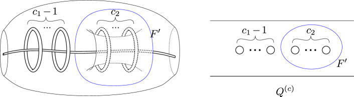
Figure 7. Case 1.a

Subcase 1.a: $I=\{1,\dots,n\}$ and $\partial N(K)\subset E(\#_{i=1}^{n}K_{i})^{(c_{1})}$. For this subcase, see Figure 7. Recall that $E(\#_{i=1}^{n}K_{i})^{(c)}=E(\#_{i=1}^{n}K_{i})^{(c_{1})}\cup_{F^{\prime}}D(c_{2})$ with $c_{1}+c_{2}=c+1$; by reordering $T_{1},\dots,T_{c}$ if necessary we may assume that $T_{1},\dots,T_{c_{1}-1}\subset\partial E(\#_{i=1}^{n}K_{i})^{(c_{1})}$ and $T_{c_{1}},\dots,T_{c}\subset\partial D(c_{2})$. Since $F^{\prime}$ is not boundary parallel $c_{2}\geq 2$; thus $c_{1}<c$. Thus $(n,c_{1})<(n,c)$ (in the lexicographic order) and hence we may apply induction to $E(\#_{i=1}^{n}K_{i})^{(c_{1})}$. Let $\Sigma_{1}^{\prime}$ be the Heegaard surface induced on $E(\#_{i=1}^{n}K_{i})^{(c_{1})}$ by the weak reduction of $\Sigma$. By assumption Conclusion 2 of Theorem 1.7 does not hold; it is easy to see that $E(\#_{i=1}^{n}K_{i})^{(c_{1})}$ fulfills the assumptions of Theorem 1.7, and since $g(\Sigma_{1}^{\prime})<g(\Sigma)$, Conclusion (2) does not hold for $E(\#_{i=1}^{n}K_{i})^{(c_{1})}$. Therefore the inductive hypothesis shows that $E(\#_{i=1}^{n}K_{i})^{(c_{1})}$ admits a Heegaard surface $\Sigma_{1}$ fulfilling the following three conditions:

1. $g(\Sigma_{1})=g(\Sigma_{1}^{\prime})$;

2. $\Sigma_{1}$ and $\Sigma_{1}^{\prime}$ induces the same partition of the components of

   $\partial E(\#_{i=1}^{n}K_{i})^{(c_{1})}\setminus\{T_{1},\dots,T_{c_{1}-1},F^{\prime},\partial N(K)\}$;

3. $\Sigma_{1}$ admits a complete system of Hopf–Haken annuli.

Denote the union of the $c_{1}-1$ Hopf–Haken annuli connecting $\partial N(\#_{i=1}^{n}K_{i})$ to $T_{1},\dots,T_{c_{1}-1}$ by $\mathcal{A}_{1}$ and the Hopf–Haken annulus connecting $\partial N(\#_{i=1}^{n}K_{i})$ to $F^{\prime}$ by $A$ (note that $c_{1}-1=0$ is possible; in that case $\mathcal{A}_{1}=\emptyset$). There exists a minimal genus Heegaard surface $\Sigma_{2}$ for $D(c_{2})$ that admits $c_{2}$ Haken annuli $A_{c_{1}},\dots,A_{c}$ so that one component of $\partial A_{i}$ is a longitude of $T_{i}$ and the other is on $F^{\prime}$ and parallel to $A\cap F^{\prime}$ there (recall Remark 4.2). We denote $\cup_{i=c_{1}}^{c}A_{i}$ by $\mathcal{A}_{2}$. As shown in Proposition 4.3, the annuli obtained by attaching a parallel copy of $A$ to each annulus of $\mathcal{A}_{2}$ union $\mathcal{A}_{1}$ are Haken annuli for the Heegaard surface obtained by amalgamating $\Sigma_{1}$ and $\Sigma_{2}$; we will denote this surface by $\hat{\Sigma}$. By construction, these annuli form a complete system of Hopf-Haken annuli for $\hat{\Sigma}$. Since $g(\hat{\Sigma})=g(\Sigma_{1})+g(\Sigma_{2})-1$ and $g(\Sigma)=g(\Sigma_{1}^{\prime})+g(\Sigma_{2})-1$, by Condition (1) above we have $g(\hat{\Sigma})=g(\Sigma)$. By construction $\Sigma$ and $\Sigma^{\prime}$ induce the same partition of the components of $\partial E(K)^{(c)}\setminus\{T_{1},\dots,T_{c},\partial N(K)\}$. Theorem 1.7 follows in Subcase 1.a.

Subcase 1.b: $I=\{1,\dots,n\}$ and $\partial N(K)\subset D(c_{2})$.

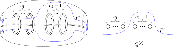
Figure 8. Subcase 1.b

For this subcase see Figure 8. Since Subcase 1.b is similar to Subcase 1.a we omit some of the easier details of the proof. As in Subcase 1.a, $F^{\prime}$ decomposes $E(\#_{i=1}^{n}K_{i})^{(c)}$ as $E(\#_{i=1}^{n}K_{i})^{(c_{1})}\cup_{F^{\prime}}D(c_{2})$ with $c_{1}+c_{2}=c+1$; we reorder $T_{1},\dots,T_{c}$ so that $T_{1},\dots,T_{c_{1}}\subset\partial E(\#_{i=1}^{n}K_{i})^{(c_{1})}$ and $T_{c_{1}+1},\dots,T_{c}\subset\partial D(c_{2})$. By induction there exists a minimal genus Heegaard surface $\Sigma_{1}$ for $E(\#_{i=1}^{n}K_{i})^{(c_{1})}$ fulfilling conditions analogous to (1)–(3) listed in Subcase 1.a. In particular, $\Sigma_{1}$ admits a complete system of $c_{1}$ Hopf–Hakn annuli, say $\mathcal{A}_{1}$, so that one boundary component of each annulus of $\mathcal{A}_{1}$ is a longitude of $T_{i}$ ($i=1,\dots,c_{1}$) and the other is a curve of $F^{\prime}$. As in Subcase 1.a, there exists a minimal genus Heegaard surface $\Sigma_{2}$ for $D(c_{2})$ admitting a system of $c_{2}$ Haken annuli (recall Remark 4.2), denoted by $\mathcal{A}_{2}\cup A$, so that $\mathcal{A}_{2}$ consists of $c_{2}-1$ annuli connecting meridians of $\partial N(\#K_{i})$ to the longitudes of $T_{c_{1}+1},\dots,T_{c}$, and $A$ connects a meridian of $\partial N(\#K_{i})$ to a curve of $F^{\prime}$; by construction, this curve is parallel to the curves of $\mathcal{A}_{1}\cap F^{\prime}$. As shown in Proposition 4.3, the annuli obtained by attaching a parallel copy of $A$ to each annulus of $\mathcal{A}_{1}$ union $\mathcal{A}_{2}$ are Haken annuli for the Heegaard surface obtained by amalgamating $\Sigma_{1}$ and $\Sigma_{2}$; we will denote this surface by $\hat{\Sigma}$. By construction, these annuli form a complete system of Hopf-Haken annuli for $\hat{\Sigma}$. As in Case 1.a, $g(\hat{\Sigma})=g(\Sigma)$ and $\hat{\Sigma}$ induces the same partition on the components of $\partial E(K)^{(c)}\setminus\{T_{1},\dots,T_{c},\partial N(K)\}$ as $\Sigma$. Theorem 1.7 follows in Subcase 1.b.

Case 2: $\emptyset\neq I\not=\{1,\dots,n\}$. See Figure 9 for this case.

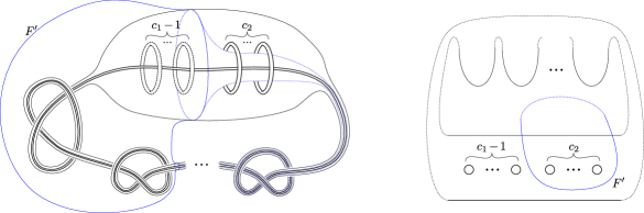
Figure 9. Case 2

Since Case 2 is similar to Subcase 1.a we omit some of the easier details of the proof. By symmetry we may assume that $\partial N(K)\subset\partial E(\#_{i\in I}K_{i})^{(c_{1})}$. Let $\Sigma_{1}^{\prime}$ and $\Sigma_{2}^{\prime}$ be the Heegaard surfaces induced on $E(\#_{i\in I}K_{i})^{(c_{1})}$ and $E(\#_{i\not\in I}K_{i})^{(c_{2})}$ (respectively) by $\Sigma$. Since both $|I|$ and $n-|I|$ are strictly less than $n$, we may apply induction to both $E(\#_{i\in I}K_{i})^{(c_{1})}$ and $E(\#_{i\not\in I}K_{i})^{(c_{2})}$. By induction, there exists a minimal genus Heegaard surfaces $\Sigma_{1}$ and $\Sigma_{2}$ for $E(\#_{i\in I}K_{i})^{(c_{1})}$ and $E(\#_{i\not\in I}K_{i})^{(c_{2})}$ (respectively) fulfilling the following three conditions:

1. $g(\Sigma_{1})=g(\Sigma_{1}^{\prime})$ and $g(\Sigma_{2})=g(\Sigma_{2}^{\prime})$;

2. $\Sigma_{1}$ induces the same partition of the components of
   $\partial E(\#_{i\in I}K_{i})^{(c_{1})}\setminus\{\partial N(K),T_{1},\dots,T_{c_{1}-1}\}$ as $\Sigma_{1}^{\prime}$; similarly, $\Sigma_{2}$ induces the same partition of the components of $\partial E(\#_{i\not\in I}K_{i})^{(c_{2})}\setminus\{T_{c_{1}},\dots,T_{c}\}$ as $\Sigma_{2}^{\prime}$.

3. $\Sigma_{1}$ admits a complete system of Hopf-Haken annuli, say $A\cup\mathcal{A}_{1}$, where $A$ connects $\partial N(K)$ to $F^{\prime}$ and the components of $\mathcal{A}_{1}$ connect $\partial N(K)$ to $T_{1},\dots,T_{c_{1}-1}$; similary $\Sigma_{2}$ admit complete systems of Hopf–Haken annuli $\mathcal{A}_{2}$ whose components connect $F^{\prime}$ to $T_{c_{1}},\dots,T_{c}$.

As shown in Proposition 4.3, the annuli obtained by attaching a parallel copy of $A$ to each annulus of $\mathcal{A}_{2}$ union $\mathcal{A}_{1}$ are Haken annuli for the Heegaard surface obtained by amalgamating $\Sigma_{1}$ and $\Sigma_{2}$; we will denote this surface by $\hat{\Sigma}$. By construction, these annuli form a complete system of Hopf-Haken annuli for $\hat{\Sigma}$. As above $g(\hat{\Sigma})=g(\Sigma)$ and $\hat{\Sigma}$ induces the same partition of the components of $\partial E(K)^{(c)}\setminus\{T_{1},\dots,T_{c},\partial N(K)\}$ as $\Sigma$. Theorem 1.7 follows in Case 2.

This completes the proof of Theorem 1.7. ∎

9. Weak reduction to swallow follow tori and calculating $g(E(K)^{(c)})$

Let $K_{1}\subset M_{1},\dots,K_{n}\subset M_{n}$ be knots in compact manifolds and $c>0$ an integer. When convenient, we will denote $\#_{i=1}^{n}K_{i}$ by $K$. Let $c_{1},\dots,c_{n}\geq 0$ be integers such that $\sum_{i=1}^{n}c_{i}=c+n-1$. By Proposition 6.3 there exist $n-1$ swallow follow tori $\mathcal{T}\subset E(K)^{(c)}$ that decompose it as $E(K)^{(c)}=\cup_{\mathcal{T}}E(K_{i})^{(c_{i})}$. By amalgamating minimal genus Heegaard surfaces for $E(K_{i})^{(c_{i})}$ we obtain a Heegaard surface for $E(K)^{(c)}$; however, it is distinctly possible that the surface obtained is not of minimal genus. This motivates the following definition:

Definition 9.1 (natural swallow follow tori).

Let $K_{1}\subset M_{1},\dots,K_{n}\subset M_{n}$ be prime knots in compact manifolds and $c\geq 0$ an integer. Let $\mathcal{T}\subset E(\#_{i=1}^{n}K_{i})^{(c)}$ be a collection of $n-1$ swallow follow tori giving the decomposition $E(\#_{i=1}^{n}K_{i})^{(c)}=\cup_{\mathcal{T}}E(K_{i})^{(c_{i})}$, for some integers $c_{i}\geq 0$. We say that $\mathcal{T}$ is natural if it is obtained from a minimal genus Heegaard surface for $E(\#_{i=1}^{n}K_{i})^{(c)}$ by iterated weak reduction; equivalently, $\mathcal{T}$ is called natural if

$$g(E(\#_{i=1}^{n}K_{i})^{(c)})=\sum_{i=1}^{n}g(E(K_{i})^{(c_{i})})-(n-1)$$

Remark.

As explained in Section 6, given any collection of $n-1$ swallow follow tori $\mathcal{T}\subset E(\#_{i=1}^{n}K_{i})^{(c)}$ that give the decomposition $E(\#_{i=1}^{n}K_{i})^{(c)}=\cup_{\mathcal{T}}E(K_{i})^{(c_{i})}$, the integers $c_{1},\dots,c_{n}$ satisfy the equation $\sum_{i=1}^{n}c_{i}=c+n-1$. We will often use this fact without reference; compare this to Proposition 6.3 where the converse was established.

Example 9.2 (Knots with no natural swallow follow tori).

In Theorem 9.4 below we prove existence of natural swallow follow tori under certain assumptions. The following example shows that this is not always the case. We first analyze basic properties of knots that admit natural swallow follow tori: let $K_{1},K_{2}\subset S^{3}$ be prime knots and $T\subset E(K_{1}\#K_{2})$ a natural swallow follow torus. By exchanging the subscripts if necessary we may assume that $T$ decomposes $E(K_{1}\#K_{2})$ as $E(K_{1})^{(1)}\cup_{T}E(K_{2})$. By definition of naturallity,

$$g(E(K_{1}\#K_{2}))=g(E(K_{1})^{(1)})+g(E(K_{2}))-1$$

It is easy to see that $g(E(K_{1})^{(1)})\geq g(E(K_{1}))$. Combining these, we see that $g(E(K_{1}\#K_{2}))\geq g(E(K_{1}))+g(E(K_{2}))-1$. Morimoto [18] constructed examples of prime knots $K_{1}$, $K_{2}$ for which $g(E(K_{1}\#K_{2}))=g(E(K_{1}))+g(E(K_{2}))-2$. We conclude that for these knots, $E(K_{1}\#K_{2})$ does not admit a natural swallow follow torus.

Example 9.3 (knots where only certain swallow follow tori are natural).

The following example is of a more subtle phenomenon. It shows that even when $E(K_{1}\#K_{2})$ does admit a natural swallow follow torus, not every swallow follow torus is natural. In this sense, the weak reduction found in Theorem 9.4 is special as it finds natural swallow follow tori.

Let $K_{MSY}\subset S^{3}$ be the knot constructed by Morimoto Sakuma and Yokota in [20] and recall the notation $2K_{MSY}=K_{MSY}\#K_{MSY}$. It was shown in [20] that $g(E(K_{MSY}))=2$ and $g(E(2K_{MSY}))=4$.

We claim that $g(E(K_{MSY})^{(1)})=3$. By [22], either $g(E(K_{MSY})^{(1)})=2$ or $g(E(K_{MSY})^{(1)})=3$. Assume for a contradiction that $g(E(K_{MSY})^{(1)})=2$. By Corollary 6.4 (with $c=0$, $c_{1}=1$, and $c_{2}=0$) we have

$$g(E(2K_{MSY}))\leq g(E(K_{MSY})^{(1)})+g(E(K_{MSY}))-1=2+2-1=3$$

a contradiction. Hence $g(E(K_{MSY})^{(1)})=3$.

Let $K$ be any non-trivial 2-bridge knot. It is well known that $g(E(K))=2$. We claim that $g(E(K_{MSY}\#K))=3$. Since tunnel number one knots are prime [21], $g(E(K_{MSY}\#K))\geq 3$. On the other hand, since $K$ admits a $(1,1)$ decomposition, by Theorem 5.4 we have that $g(E(K)^{(1)})=2$. As above, Corollary 6.4 gives

$$g(E(K_{MSY}\#K))\leq g(E(K_{MSY}))+g(E(K)^{(1)})-1=2+2-1=3$$

Hence $g(E(K_{MSY}\#K))=3$.

$E(K_{MSY}\#K)$ admits two swallow follow tori, say $T_{1}$ and $T_{2}$, that decompose it as follows:

1. $g(E(K_{MSY}\#K))=E(K_{MSY})^{(1)}\cup_{T_{1}}E(K)$, and

2. $g(E(K_{MSY}\#K))=E(K_{MSY})\cup_{T_{2}}E(K)^{(1)}$.

In each case, amalgamating minimal genus Heegaard surfaces for the manifolds appearing on the right hand side yields a Heegaard surface for $E(K_{MSY}\#K)$ whose genus fulfills (Lemma 2.2):

1. $g(E(K_{MSY})^{(1)})+g(E(K))-g(T_{1})=3+2-1=4,$ and

2. $g(E(K_{MSY}))+g(E(K)^{(1)})-g(T_{2})=2+2-1=3.$

We conclude that $T_{2}$ is a natural swallow follow torus but $T_{1}$ is not.

In this section we show that if $K_{i}$ is m-small for all $i$, then any minimal genus Heegaard surface for $E(\#_{i=1}^{n}K_{i})^{(c)}$ weakly reduces to a natural collection of swallow follow tori. The statement of Theorem 9.4 is more general and allows for non-minimal genus Heegaard surfaces.

Theorem 9.4.

Let $K_{i}\subset M_{i}$ be prime knots in compact manifolds so that $E(K_{i})$ not homeomorphic to $T^{2}\times I$, $E(K_{i})$ is irreducible, and $\partial N(K_{i})$ is incompressible in $E(K_{i})$. Let $\Sigma$ be a (not necessarily minimal genus) Heegaard surface for $E(\#_{i=1}^{n}K_{i})^{(c)}$. Then one of the following holds:

1. $\Sigma$ admits iterated weak reductions that yield a collection of $n-1$ swallow follow tori, say $\mathcal{T}$, giving the decomposition

   $$E(\#_{i=1}^{n}K_{i})^{(c)}=\cup_{\mathcal{T}}E(K_{i})^{(c_{i})}$$

   where $c_{1},\dots,c_{n}$ are integers such that $\Sigma_{i=1}^{n}c_{i}=c+n-1$.

2. For some $i$, $K_{i}$ admits an essential meridional surface $S$ with $\chi(S)\geq 6-2g(\Sigma)$.

The main corollary of Theorem 9.4 allows us to calculate $g(E(\#_{i=1}^{n}K_{i})^{(c)})$ in terms of $g(E(K_{i})^{(c_{i})})$.

Corollary 9.5.

In addition to the assumptions of Theorem 9.4, suppose that no $K_{i}$ admits an essential meridional surface $S$ with $\chi(S)\geq 6-2g(E(\#_{i=1}^{n}K_{i})^{(c)})$. Then $E(\#_{i=1}^{n}K_{i})^{(c)}$ admits a natural collection of $n-1$ swallow follow tori; equivalently, there exist integers $c_{1},\dots,c_{n}\geq 0$ so that $\sum_{i=1}^{n}c_{i}=c+n-1$ and

$$g(E(\#_{i=1}^{n}K_{i})^{(c)})=\Sigma_{i=1}^{n}g(E(K_{i})^{(c_{i})})-(n-1)$$

Proof.

Apply Theorem 9.4 to a minimal genus Heegaard splitting of $E(\#_{i=1}^{n}K_{i})^{(c)}$ and apply Lemma 2.2. ∎

We get:

Corollary 9.6.

In addition to the assumptions of Theorem 9.4, suppose that no $K_{i}$ admits an essential meridional surface $S$ with $\chi(S)\geq 6-2g(E(\#_{i=1}^{n}K_{i})^{(c)})$. Then

$$g(E(\#_{i=1}^{n}K_{i})^{(c)})=\min\Big{\{}\sum_{i=1}^{n}g(E(K_{i})^{(c_{i})})-(n-1)\Big{\}}$$

where the minimum is taken over all integers $c_{1},\dots,c_{n}\geq 0$ with $\Sigma c_{i}=c+n-1$.

Proof.

By Corollary 6.4, for any collection of integers $c_{1},\dots,c_{n}$ such that $\sum_{i=1}^{n}c_{i}=c+n-1$ we have that

$$g(E(\#_{i=1}^{n}K_{i})^{(c)})\leq\sum_{i=1}^{n}g(E(K_{i})^{(c_{i})})-(n-1)$$

and by Corollary 9.5, there exist integers $c_{1},\dots,c_{n}$ for which equality holds. The corollary follows. ∎

Proof of Theorem 9.4.

We induct on $(n,c)$ ordered lexicographically. Recall that in the beginning of the proof of Theorem 1.7 we showed that $(n,c)$ is well defined. If $n=1$ there is nothing to prove; assume from now on $n>1$.

Assume Conclusion (2) of Theorem 9.4 does not hold, that is, for each $i$, $E(K_{i})$ does not admit an essential meridional surface $S$ with $\chi(S)\geq 6-2g(\Sigma)$. Then by the Swallow Follow Torus Theorem [13, Theorem 4.1] $\Sigma$ weakly reduces to a swallow follow torus, say $T$. $T$ decomposes $E(\#_{i=1}^{n}K_{i})^{(c)}$ as $E(K_{I})^{(c_{I})}\cup_{T}E(K_{J})^{(c_{J})}$, where $I\subseteq\{1,\dots,n\}$ (possibly empty), $c_{I}+c_{J}=c+1$, $K_{I}=\#_{i\in I}K_{i}$, and $K_{J}=\#_{i\not\in I}K_{i}$. Denote the Heegaard surfaces induced on $E(K_{I})^{(c_{I})}$ and $E(K_{J})^{(c_{J})}$ by $\Sigma_{I}$ and $\Sigma_{J}$, respectively.

Case One: $\emptyset\neq I\neq\{1,\dots,n\}$: In this case both $E(K_{I})^{(c_{I})}$ and $E(K_{J})^{(c_{J})}$ are exteriors of knots with strictly less than $n$ prime factors and hence we may apply induction to both. Since $g(\Sigma_{I})<g(\Sigma)$, conclusion (2) of Theorem 9.4 does not hold for $E(K_{I})^{(c_{I})}$. Hence, by induction, $\Sigma_{I}$ admits iterated weak reduction that yields a collection of $|I|-1$ swallow follow tori (say $\mathcal{T}_{I}\subset E(K_{I})^{(c_{I})}$) so that the following conditions hold:

1. $\mathcal{T}_{I}$ decompose $E(K_{I})^{(c_{I})}$ as $\cup_{\mathcal{T}_{I}}E(K_{i})^{(c_{i})}$ (for $i\in I$),

2. $\sum_{i\in I}c_{i}=c_{I}+|I|-1$.

Similarly, $\Sigma_{J}$ admits iterated weak reduction that yields a collection of $(n-|I|)-1$ swallow follow tori (say $\mathcal{T}_{J}\subset E(K_{J})^{(c_{J})}$) so that the following conditions hold:

1. $\mathcal{T}_{J}$ decompose $E(K_{J})^{(c_{J})}$ as $\cup_{\mathcal{T}_{J}}E_{i}^{(c_{i})}$ (for $i\not\in I$),

2. $\sum_{i\not\in I}c_{i}=c_{J}+(n-|I|)-1$.

Thus after iterated weak reduction of $\Sigma$ we obtain $\mathcal{T}=T\cup\mathcal{T}_{I}\cup\mathcal{T}_{J}$. By the above, $\mathcal{T}$ decomposes $E(\#_{i=1}^{n}K_{i})^{(c)}$ as $\cup_{\mathcal{T}}E(K_{i})^{(c_{i})}$, so that $\sum_{i=1}^{n}c_{i}=\sum_{i\in I}c_{i}+\sum_{i\not\in I}c_{i}=c_{I}+|I|-1+c_{J}+(n-|I|)-1=c+n-1$ (recall that $c_{I}+c_{J}=c+1$). This proves Theorem 9.4 in Case One.

Case Two: $I=\emptyset$ or $I=\{1,\dots,n\}$. By symmetry we may assume that $I=\{1,\dots,n\}$. In that case $E(K_{J})^{(c_{J})}\cong D(c_{J})$, a disk with $c_{J}$ holes cross $S^{1}$, and $T$ gives the decomposition:

$$E(\#_{i=1}^{n}K_{i})^{(c)}=E(\#_{i=1}^{n}K_{i})^{(c_{I})}\cup_{T}D(c_{J})$$

Since $T$ is essential (and in particular, not boundary parallel) $c_{J}\geq 2$. Since $c_{I}+c_{J}=c+1$, we have that $c_{I}<c$. Thus the complexity of $E(\#_{i=1}^{n}K_{i})^{(c_{I})}$ is $(n,c_{I})<(n,c)$ and we may apply induction to $E(\#_{i=1}^{n}K_{i})^{(c_{I})}$. Let $\Sigma_{I}$ be the Heegaard surface for $E(\#_{i=1}^{n}K_{i})^{(c_{I})}$ induced by weak reduction. By induction, $\Sigma_{I}$ admits a repeated weak reduction that yields a system of $n-1$ swallow follow tori, say $\mathcal{T}_{I}$, that decomposes $E(\#_{i=1}^{n}K_{i})^{(c_{I})}$ as

$$E(\#_{i=1}^{n}K_{i})^{(c_{I})}=\cup_{\mathcal{T}_{I}}E(K_{i})^{(c_{i})}$$

with $\sum_{i=1}^{n}c_{i}=c_{I}+n-1$. Let $T^{\prime}$ be a component of $\mathcal{T}_{I}$. Then $T^{\prime}$ decomposes $E(\#_{i=1}^{n}K_{i})^{(c_{I})}$ as $E(\#_{i=1}^{n}K_{i})^{(c_{I})}=E(\#_{i\in I^{\prime}}K_{i})^{(b_{1})}\cup_{T^{\prime}}E(\#_{i\not\in I^{\prime}}K_{i})^{(b_{2})}$, for some $I^{\prime}\subseteq\{1,\dots,n\}$ and some integers $b_{1},b_{2}\geq 0$ with $b_{1}+b_{2}=c_{I}+1$. Since $T^{\prime}\subset\mathcal{T}_{I}$, we have that $\emptyset\neq I^{\prime}\neq\{1,\dots,n\}$. By Proposition 2.3, we see that $\Sigma$ weakly reduce to $T^{\prime}$. This reduces Case Two to Case One, completing the proof of Theorem 9.4. ∎

10. Calculating the growth rate of m-small knots

In this final section we complete the proof of Theorem 1.2. Let $K\subset M$ be an m-small admissible knot in a compact manifold. Recall the notation $nK$ and $E(K)^{(c)}$.

The difference between $g(E(K)^{(c)})$ and $g(E(K))+c$ is measured by a function denoted ${f_{K}}$ that plays a key role our work:

Definition 10.1.

Given a knot $K$, we define the function ${f_{K}}:\mathbb{Z}_{\geq 0}\to\mathbb{Z}$ to be

$${f_{K}}(c)=g(E(K))+c-g(E(K)^{(c)})$$

We immediately see that ${f_{K}}$ has the following properties, which we will often use without reference:

1. ${f_{K}}(0)=0$.

2. For $c\geq 0$, ${f_{K}}(c)\leq{f_{K}}(c+1)\leq{f_{K}}(c)+1$: this follows from the fact (proved in [22]) that for all $c\geq 0$, $g(E(K)^{(c)})\leq g(E(K)^{(c+1)})\leq g(E(K)^{(c)})+1$

3. For $c\geq 0$, $0\leq{f_{K}}(c)\leq c$ (follows easily from (2)).

Before proceeding, we rephrase Corollaries 9.5 and 9.6 in terms of ${f_{K}}$:

Corollary 10.2.

Let $K\subset M$ be a knot in a compact manifold and let $n$ be a positive integer. Suppose that $E(K)$ does not admit a meridional essential surface $S$ with $\chi(S)\geq 6-2g(E(nK))$. Then there exist integers $c_{1}\dots,c_{n}\geq 0$ with $\Sigma c_{i}=n-1$ so that:

$$g(E(nK))=ng(E(K))-\sum_{i=1}^{n}{f_{K}}(c_{i})$$

Proof.

By Corollary 9.5 (with $c=0$) there exist $c_{1},\dots,c_{n}\geq 0$ with $\Sigma c_{i}=n-1$, so that $g(E(nK))=\sum_{i=1}^{n}g(E(K)^{(c_{i})})-(n-1)$. We get:

$$g(E(nK)) = \Big{[}\sum_{i=1}^{n}g(E(K)^{(c_{i})})\Big{]}-(n-1)$$

$$= \Big{[}\sum_{i=1}^{n}g(E(K))+c_{i}-{f_{K}}(c_{i})\Big{]}-(n-1)$$

$$= ng(E(K))+\Big{[}\sum_{i=1}^{n}c_{i}\Big{]}-\Big{[}\sum_{i=1}^{n}{f_{K}}(c_{i})\Big{]}-(n-1)$$

$$= ng(E(K))+(n-1)-\Big{[}\sum_{i=1}^{n}{f_{K}}(c_{i})\Big{]}-(n-1)$$

$$= ng(E(K))-\sum_{i=1}^{n}{f_{K}}(c_{i})$$

∎

A similar argument shows that Corollary 9.6 gives:

Corollary 10.3.

Let $K\subset M$ be a knot in a compact manifold and let $n$ be a positive integer. Suppose that $E(K)$ does not admit a meridional essential surface $S$ with $\chi(S)\geq 6-2g(E(nK))$. Then we have:

$$g(E(nK)) = \min\big{\{}ng(E(K))-\Sigma_{i=1}^{n}{f_{K}}(c_{i})\big{\}}$$

$$= ng(E(K))-\max\big{\{}\Sigma_{i=1}^{n}{f_{K}}(c_{i})\big{\}}$$

where the minimum and maximum are taken over all integers $c_{1},\dots,c_{n}\geq 0$ with $\sum_{i=1}^{n}c_{i}=n-1$.

Recall (Notation 1.1) that we denote $g(E(K))-g(M)$ by $g$ and the bridge indices of $K$ with respect to Heegaard surfaces of genus $g(E(K))-i$ by $b_{i}^{*}$ ($=1,\dots,g$), so that $0<b^{*}_{1}<\dots<b^{*}_{i}<\dots<b^{*}_{g}$. We formally set $b_{0}^{*}=0$ and $b_{g+1}^{*}=\infty$. Note that these properties imply that for every $c\geq 0$ there is a unique index $i$ ($0\leq i\leq g$), depending on $c$, so that $b^{*}_{i}\leq c<b^{*}_{i+1}$; we will use this fact below without reference.

In the following proposition we calculate ${f_{K}}(c)$ when $E(K)$ does not admit an essential meridional surface $S$ with $\chi(S)\geq 6-2g(E(K)^{(c)})$.

Proposition 10.4.

Let $K$ be a knot and $c\geq 0$ an integer. Let $0\leq i\leq g$ be the unique index for which $b^{*}_{i}\leq c<b^{*}_{i+1}$. Then ${f_{K}}(c)\geq i$. If in addition $E(K)$ does not admit an essential meridional surface $S$ with $\chi(S)\geq 6-2g(E(K)^{(c)})$ then equality holds:

$${f_{K}}(c)=i$$

Proof of Proposition 10.4.

We first prove that ${f_{K}}(c)\geq i$ holds for any knot. Since ${f_{K}}$ is a non-negative function we may assume $i\geq 1$. By the definition of $b^{*}_{i}$, $K$ admits a ($g(E(K))-i$, $b^{*}_{i}$) decomposition. Since $c\geq b^{*}_{i}$, $K$ admits a $(g(E(K))-i,c)$ decomposition. By Corollary 5.6 we have that $g(E(K)^{(c)})\leq g(E(K))-i+c$. Therefore, ${f_{K}}(c)=g(E(K))+c-g(E(K)^{(c)})\geq g(E(K))+c-(g(E(K))-i+c)=i$.

Next we assume, in addition, that $E(K)$ does not admit an essential meridional surface $S$ with $\chi(S)\geq 6-2g(E(K)^{(c)})$. We will complete the proof of the proposition by showing that ${f_{K}}(c)<i+1$; suppose for a contradiction that ${f_{K}}(c)\geq i+1$. Thus $g(E(K)^{(c)})=g(E(K))+c-{f_{K}}(c)\leq g(E(K))+c-(i+1)$.

Assume first that $i=g$. Then by Corollary 8.1 (with $g(E(K))+c-(g+1)$ corresponding to $h$) we see that $k$ admits a $(g(E(K))+c-(g+1)-c,c)$ decomposition. In particular, $M$ admits a Heegaard surface of genus $(g(E(K)))+c-(g+1)-c$. Hence we see:

$$g(M) \leq (g(E(K))+c-(g+1)-c$$

$$= g(E(K))-g-1$$

$$= g(E(K))-(g(E(K))-g(M))-1$$

$$= g(M)-1$$

This contradiction completes the proof when $i=g$.

Next assume that $0\leq i<g$. Applying Corollary 8.1 again (with $g(E(K))+c-(i+1)$ corresponding to $h$ in Corollary 8.1) we see that $K$ admits a $(g(E(K))-(i+1),c)$ decomposition. By definition, $b^{*}_{i+1}$ is the smallest integer so that $K$ admits a $(g(E(K))-(i+1),b^{*}_{i+1})$ decomposition; hence $c\geq b^{*}_{i+1}$. This contradicts our choice of $i$ in the statement of the proposition, showing that ${f_{K}}(c)<i+1$. This completes the proof of Proposition 10.4. ∎

As an illustration of Proposition 10.4, let $K$ be an m-small knot in $S^{3}$. Suppose that $g=3$, $b^{*}_{1}=5$, $b^{*}_{2}=7$, and $b^{*}_{3}=23$. (We do not know if a knot with these properties exists.) Then:

$${f_{K}}(c)=\left\{\begin{array}[]{l}0\hskip 72.26999pt0\leq c\leq 4\\ 1\hskip 72.26999pt5\leq c\leq 6\\ 2\hskip 72.26999pt7\leq c\leq 22\\ 3\hskip 72.26999pt23\leq c\\ \end{array}\right.$$

Not much is known about ${f_{K}}$ for knots that are not m-small:

Question 10.5.

Does there exist a knot $K$ in a manifold $M$ with unbounded ${f_{K}}$? Does there exist a knot $K$ with ${f_{K}}(c)>g(E(K))-g(M)$ (for sufficiently large $c$)? What can be said about the behavior of the function ${f_{K}}$?

With the preparation complete, we are now ready to prove Theorem 1.2.

Proof of Theorem 1.2.

Fix the notation of Theorem 1.2. Since the upper bound was obtained in Proposition 7.1, we assume from now on that $K$ is m-small. By Corollary 10.3, $g(E(nK))=ng(E(K))-\max\{\Sigma_{i=1}^{n}{f_{K}}(c_{i})\}$, where the maximum is taken over all integers $c_{1},\dots,c_{n}\geq 0$ with $\sum_{i=1}^{n}c_{i}=n-1$.

Fix $n$ and let $c_{1},\dots,c_{n}\geq 0$ be integers with $\sum_{i=1}^{n}c_{i}=n-1$ that maximize $\Sigma_{i=1}^{n}{f_{K}}(c_{i})$.

Lemma 10.6.

We may assume that the sequence $c_{1},\dots,c_{n}$ fulfills the following conditions for some $1\leq l\leq n$:

1. $c_{i}\geq c_{i+1}$ ($i=1,\dots,n-1$).

2. For $i\leq l$, $c_{i}\in\{b_{1}^{*},\dots,b_{g}^{*}\}$.

3. $c_{l+1}<b_{1}^{*}$.

4. For $i>l+1$, $c_{i}=0$.

Proof.

By reordering the indices if necessary we may assume (1) holds.

Let $l$ be the largest index for which ${f_{K}}(c_{l})\neq 0$. For $i=1,\dots,l$, let $0\leq j(i)\leq g$ be the unique index for which $b^{*}_{j(i)}\leq c_{i}<b^{*}_{j(i)+1}$ (recall that we set $b^{*}_{0}=0$ and $b_{g+1}^{*}=\infty$). Define $c^{\prime}_{1},\dots,c^{\prime}_{n}$ as follows:

1. For $i\leq l$, set $c^{\prime}_{i}=b^{*}_{j(i)}$ (in other words, $c_{i}^{\prime}$ is the largest $b_{j}^{*}$ that does not exceed $c_{i}$).

2. Set $c^{\prime}_{l+1}=n-1-(\sum_{i=1}^{l}c^{\prime}_{i})$.

3. For $i>l+1$ set $c^{\prime}_{i}=0$.

By Proposition 10.4, for $i\leq l$, ${f_{K}}(c_{i})={f_{K}}(b^{*}_{j(i)})={f_{K}}(c_{i}^{\prime})$. We get :

$$\sum_{i=1}^{n}{f_{K}}(c^{\prime}_{i}) = \sum_{i=1}^{l}{f_{K}}(c^{\prime}_{i})+\sum_{i=l+1}^{n}{f_{K}}(c^{\prime}_{i})$$

$$= \sum_{i=1}^{l}{f_{K}}(c_{i})+\sum_{i=l+1}^{n}{f_{K}}(c^{\prime}_{i})$$

$$\geq \sum_{i=1}^{l}{f_{K}}(c_{i})$$

$$= \sum_{i=1}^{n}{f_{K}}(c_{i}).$$

(For the last equality, recall that ${f_{K}}(c_{i})=0$ for $i>l$.)

Since $c_{1},\dots,c_{n}$ maximizes $\sum_{i=1}^{n}{f_{K}}(c_{i})$, we conclude that $\sum_{i=1}^{n}{f_{K}}(c_{i})=\sum_{i=1}^{n}{f_{K}}(c_{i}^{\prime})$ and hence ${f_{K}}(c^{\prime}_{l+1})=0$; thus $c_{l+1}^{\prime}<b_{1}^{*}$. Thus $c^{\prime}_{1},\dots,c^{\prime}_{n}$ is a maximizing sequence; it is easy to see that it fulfills conditions (1)–(4). ∎

We will denote the $n^{\rm th}$ term of the defining sequence of the growth rate by $S_{n}$, that is:

$$S_{n}=\frac{g(E(nK))-ng(E(K))+n-1}{n-1}$$

By Corollary 10.3 the following holds:

(2) $$S_{n}=1-\frac{\max\{\Sigma_{i=1}^{n}{f_{K}}(c_{i})\}}{n-1}$$

In order to bound $S_{n}$ below we need to understand the following optimization problem, where here we are assuming that the maximizing sequence fulfills the conditions listed in Lemma 10.6, and in particular, ${f_{K}}(c_{i})=0$ for $i>l$.

Problem 10.7.

Find non negative integers $l$ and $c_{1},\dots,c_{l}$ that maximize $\sum_{i=1}^{l}{f_{K}}(c_{i})$ subject to the constraints:

1. $\sum_{i=1}^{l}c_{i}\leq n-1$

2. $c_{i}\in\{b^{*}_{1},\dots,b^{*}_{g}\}$ (for $1\leq i\leq l$).

For $i=1,\dots,g$, let $k_{i}$ be the number of times that $b^{*}_{i}$ appears in $c_{1},\dots,c_{l}$. By Proposition 10.4, ${f_{K}}(b^{*}_{i})=i$; thus Problem 10.7 can be rephrased as follows:

Problem 10.8.

Maximize $\sum_{i=1}^{g}k_{i}i$ subject to the constraints:

1. $\sum_{i=1}^{g}k_{i}b^{*}_{i}\leq n-1$

2. $k_{i}$ is a non-negative integer

We first solve this optimization problem over $\mathbb{R}$; we use the variables $x_{1},\dots,x_{g}$ instead of $k_{1},\dots,k_{g}$.

Problem 10.9.

Given $n\in\mathbb{R}$, $n>1$, maximize $\sum_{i=1}^{g}x_{i}i$ subject to the constraints

1. $\sum_{i=1}^{g}x_{i}b^{*}_{i}\leq n-1$

2. $x_{1}\geq 0,\dots,x_{g}\geq 0$

It is easy to see that for any sequence $x_{1},\dots,x_{g}$ that realizes maximum we have that $\sum_{i=1}^{g}x_{i}b^{*}_{i}=n-1$, for otherwise we can increase the value of $x_{1}$, thus increasing $\sum_{i=1}^{g}x_{i}i$ and contradicting maximality. Problem 10.9 is an elementary linear programming problem (known as the standard maximum problem) and is solved using the simplex method which gives:

Lemma 10.10.

There is a (not necessarily unique) index $i_{0}$, which is independent of $n$, such that a solution of Problem 10.9 is given by

$$x_{i_{0}}=\frac{n-1}{b_{i_{0}}^{*}},\ \ \ \ x_{i}=0(i\neq i_{0})$$

Hence the maximum is

$$\frac{(n-1)i_{0}}{b_{i_{0}}^{*}}$$

Proof of Lemma 10.10.

The notation used in this proof was chosen to be consistent with notation often used in linear programming texts. Let ${\bf\overrightarrow{N}},{\bf\overrightarrow{F}}$ and $\vec{x}\in\mathbb{R}^{g}$ denote the following vectors

$${\bf\overrightarrow{N}}=(b_{1}^{*},\dots,b_{g}^{*}),\ \ \ {\bf\overrightarrow{F}}=(1,\dots,g),\ \mbox{ and }\ \vec{x}=(x_{1},\dots,x_{g})$$

For $n\in\mathbb{R}$, $n>1$, let $\Delta_{n}$ be

$$\Delta_{n}=\{\vec{x}\in\mathbb{R}^{g}\ |{\bf\overrightarrow{N}}\cdot\vec{x}=n-1,x_{1}\geq 0,\dots,x_{g}\geq 0\}$$

Note that $\Delta_{n}$ is a simplex and its codimension $k$ faces are obtained by setting $k$ variables to zero. Problem 10.9 can be stated as:

$$\mbox{maximize }\ \ {\bf\overrightarrow{F}}\cdot\vec{x},\ \ \mbox{ subject to }\ \ \vec{x}\in\Delta_{n}$$

Since the gradient of ${\bf\overrightarrow{F}}\cdot\vec{x}$ is ${\bf\overrightarrow{F}}$ and the normal to $\Delta_{n}$ is ${\bf\overrightarrow{N}}$, the gradient of the restriction of ${\bf\overrightarrow{F}}\cdot\vec{x}$ to ${\Delta_{n}}$ is the projection

$${\bf\overrightarrow{P}}={\bf\overrightarrow{F}}-\frac{{\bf\overrightarrow{F}}\cdot{\bf\overrightarrow{N}}}{|{\bf\overrightarrow{N}}|^{2}}{\bf\overrightarrow{N}}$$

Note that ${\bf\overrightarrow{P}}$ is independent of $n$. The maximum of ${\bf\overrightarrow{N}}\cdot\vec{x}$ on ${\Delta_{n}}$ is found by moving along $\Delta_{n}$ in the direction of ${\bf\overrightarrow{P}}$. This shows that the maximum is obtained along a face defined by setting some of the variables to zero, and the variables set to zero are independent of $n$. Lemma 10.10 follows by picking $i_{0}$ to be one of the variables not set to zero. ∎

Fix an index $i_{0}$ as in Lemma 10.10. If $b^{*}_{i_{0}}|n-1$ then the maximum (over $\mathbb{R}$) found in Lemma 10.10 is in fact an integer and hence is also the maximum for Problem 10.7. This allows us to calculate $S_{n}$ in this case:

Lemma 10.11.

If $b^{*}_{i_{0}}|n-1$ then $S_{n}=1-{i_{0}}/{b^{*}_{i_{0}}}$.

Proof.

$$S_{n}=1-\frac{\max\{\Sigma_{i=1}^{n}{f_{K}}(c_{i})\}}{n-1}=1-\frac{(n-1)i_{0}}{(n-1)b_{i_{0}}^{*}}=1-\frac{i_{0}}{b_{i_{0}}^{*}}$$

∎

We now turn our attention to the general case, where $b^{*}_{i_{0}}$ may not divide $n-1$. We will only consider values of $n$ for which $n>b_{i_{0}}^{*}$. As in Section 7, let $k_{i_{0}}$ and $r$ be the quotient and remainder when dividing $n-1$ by $b_{i_{0}}^{*}$, so that

(3) $$n-1=k_{i_{0}}b_{i_{0}}^{*}+r,\ \ \ \\ \ 0\leq r<b_{i_{0}}^{*}$$

Let $c_{j}\geq 0$ ($1\leq j\leq n$) be integers with $\sum_{j=1}^{n}c_{j}=n-1$ that maximize $\sum_{j=1}^{n}{f_{K}}(c_{j})$. We will denote $n-r$ by $n^{\prime}$. Let $c_{j}^{\prime}\geq 0$ ($1\leq j\leq n^{\prime}$) be integers with $\sum_{j=1}^{n^{\prime}}c^{\prime}_{j}=n^{\prime}-1$ that maximize $\sum_{j=1}^{n^{\prime}}{f_{K}}(c^{\prime}_{j})$.

Claim 10.12.

$\sum_{j=1}^{n}{f_{K}}(c_{j})\leq\sum_{j=1}^{n^{\prime}}{f_{K}}(c^{\prime}_{j})+r$.

Proof.

Starting with the sequence $c_{1},\dots,c_{n}$, we obtain a new sequence by subtracting one from exactly one $c_{j}$ (with $c_{j}>0$). Let $c_{j}^{\prime\prime\prime}$ be a sequence of non negative integers obtained by repeating this process $r$ times. Then $\sum_{j=1}^{n}c_{j}^{\prime\prime\prime}=n-1-r=n^{\prime}-1$. Let $c_{j}^{\prime\prime}$ be the sequence obtained from $c_{j}^{\prime\prime\prime}$ by removing $r$ zeros (note that this is possible as there indeed are at least $r$ zeros). We get:

$$\sum_{j=1}^{n^{\prime}}{f_{K}}(c^{\prime}_{j})+r \geq\sum_{j=1}^{n^{\prime}}{f_{K}}(c^{\prime\prime}_{j})+r \mbox{ since }c_{j}^{\prime}\mbox{ maximizes}$$

$$=\sum_{j=1}^{n}{f_{K}}(c^{\prime\prime\prime}_{j})+r \mbox{ since }{f_{K}}(0)=0$$

$$\geq\sum_{j=1}^{n}{f_{K}}(c_{j}) \mbox{ since }{f_{K}}(c)+1\geq{f_{K}}(c+1)$$

This proves Claim 10.12. ∎

Note that $b_{i_{0}}^{*}|n^{\prime}-1$ and so we may apply Lemma 10.11 to calculate $S_{n^{\prime}}$. We get (in the first line we use Equation (2) from Page 2):

$$S_{n} =1-\frac{\max\{\Sigma_{i=1}^{n}f(c_{i})\}}{n-1} \mbox{Equation}~{}(\ref{eq:S_n})\mbox{ for }S_{n}$$

$$\geq 1-\frac{\max\{\Sigma_{j=1}^{n^{\prime}}f(c^{\prime}_{j})+r\}}{n-1}$$ Claim 10.12

$$=1-\frac{n^{\prime}-1}{n-1}\frac{\max\{\Sigma_{j=1}^{n^{\prime}}f(c^{\prime}_{j})\}}{n^{\prime}-1}-\frac{r}{n-1}$$

$$=\frac{n^{\prime}-1}{n-1}\Big{(}1-\frac{\max\{\Sigma_{j=1}^{n^{\prime}}f(c^{\prime}_{j})\}}{n^{\prime}-1}\Big{)}+\Big{(}1-\frac{n^{\prime}-1}{n-1}\Big{)}-\frac{r}{n-1}$$

$$=\frac{n^{\prime}-1}{n-1}S_{n^{\prime}}+\Big{(}1-\frac{n^{\prime}-1}{n-1}\Big{)}-\frac{r}{n-1} \mbox{Equation}~{}(\ref{eq:S_n})\mbox{ for }S_{n^{\prime}}$$

$$=\frac{n^{\prime}-1}{n-1}\Big{(}1-\frac{i_{0}}{b^{*}_{i_{0}}}\Big{)}+\Big{(}1-\frac{n^{\prime}-1}{n-1}\Big{)}-\frac{r}{n-1}$$ Lemma10.11

$$=\frac{n^{\prime}-1}{n-1}\Big{(}1-\frac{i_{0}}{b^{*}_{i_{0}}}\Big{)}+\Big{(}1-\frac{n^{\prime}+r-1}{n-1}\Big{)}$$

$$=\frac{n-r-1}{n-1}\Big{(}1-\frac{i_{0}}{b^{*}_{i_{0}}}\Big{)} \mbox{Substituting }n^{\prime}=n-r$$

Recall that in the proof of Proposition 7.1 (see Page 1) we proved Equation (1) which says (recall that $k_{i_{0}}$ was defined in Equation (3) above):

$$S_{n}<1-\frac{i_{0}}{b_{i_{0}}^{*}}\frac{k_{i_{0}}}{k_{i_{0}}+1}$$

Combining these facts we obtain:

$$\frac{n-r-1}{n-1}\Big{(}1-\frac{i_{0}}{b^{*}_{i_{0}}}\Big{)}\leq S_{n}<1-\frac{i_{0}}{b_{i_{0}}^{*}}\frac{k_{i_{0}}}{k_{i_{0}}+1}$$

By Equation (3) above, $r<b^{*}_{i_{0}}$ and $\lim_{n\to\infty}k_{i_{0}}=\infty$. We conclude that as $n\to\infty$ both bounds limit on $1-i_{0}/b^{*}_{i_{0}}$, and thus $\lim_{n\to\infty}S_{n}$ exists and equals $1-i_{0}/b^{*}_{i_{0}}$.

This completes the proof of Theorem 1.2. ∎

References

- [1] Kenneth L Baker, Tsuyoshi Kobayashi, and Yo’av Rieck The spectrum of the growth rate of the tunnel number is infinite. Preprint, 2015.
- [2] R. Sean Bowman, Scott A. Taylor, and A. Zupan. Bridge spectra of twisted torus knots. Int. Math. Res. Notices, doi: 10.1093/imrn/rnu162, 2014.
- [3] A. J. Casson and C. McA. Gordon. Reducing Heegaard splittings. Topology Appl., 27(3):275–283, 1987.
- [4] Wolfgang Haken. Some results on surfaces in -manifolds. In Studies in Modern Topology, pages 39–98. Math. Assoc. Amer. (distributed by Prentice-Hall, Englewood Cliffs, N.J.), 1968.
- [5] John Hempel. -Manifolds. Princeton University Press, Princeton, N. J., 1976. Ann. of Math. Studies, No. 86.
- [6] Ichihara, Kazuhiro and Saito, Toshio. Knots with arbitrarily high distance bridge decompositions. Bull. Korean Math. Soc., 50 (2013), no. 6, 1989–2000.
- [7] William Jaco. Lectures on three-manifold topology, volume 43 of CBMS Regional Conference Series in Mathematics American Mathematical Society, Providence, R.I., 1980.
- [8] W. Jaco, and P.Shalen. Seifert fibered spaces in 3-manifolds, Mem. Amer. Math. Soc., 21 (1979), no.220
- [9] K. Johannson, Homotopy equivalences of 3-manifolds, Lecture Notes in Mathematics 761. Springer, (1979).
- [10] Kim, Soo Hwan. The tunnel number one knot with bridge number three is a -knot. Kyungpook Math. J., 45(1):67–71, 2005.
- [11] Tsuyoshi Kobayashi and Yo’av Rieck. Local detection of strongly irreducible Heegaard splittings via knot exteriors. Topology Appl., 138(1-3):239–251, 2004.
- [12] Tsuyoshi Kobayashi and Yo’av Rieck. On the growth rate of tunnel number of knots, Journal für die reine und angewandte Mathematik 592 (2006) 63–78.
- [13] Tsuyoshi Kobayashi and Yo’av Rieck. Heegaard genus of the connected sum of -small knots, Comm. Anal. Geom. 5 (2006) 1037–1077.
- [14] Tsuyoshi Kobayashi and Yo’av Rieck. Knots with and and Morimoto’s Conjecture, Topology and its Appl. , 156(2009) 1114–1117.
- [15] Tsuyoshi Kobayashi and Yo’av Rieck. Knot exteriors with additive Heegaard genus and Morimoto’s conjecture. Algebr. Geom. Topol. , 8 (2008), no. 2, 953–969.
- [16] T.Kobayashi, T.Saito. Destabilizing Heegaard splittings of knot exteriors Topology and its Appl. , 157(1):202–212, 2010.
- [17] Katura Miyazaki. Conjugation and the prime decomposition of knots in closed, oriented -manifolds. Trans. Amer. Math. Soc., 313(2):785–804, 1989.
- [18] Kanji Morimoto. There are knots whose tunnel numbers go down under connected sum. Proc. Amer. Math. Soc., 123(11):3527–3532, 1995.
- [19] Kanji Morimoto. Essential surfaces in the exteriors of torus knots with twists on 2-strands. Available at http://morimoto.ii-konan.jp/TKSML.pdf.
- [20] Kanji Morimoto, Makoto Sakuma, and Yoshiyuki Yokota. Examples of tunnel number one knots which have the property “”. Math. Proc. Cambridge Philos. Soc., 119(1):113–118, 1996.
- [21] Norwood, F. H. Every two-generator knot is prime. Proc. Amer. Math. Soc., 86(1):143–147, 1982.
- [22] Yo’av Rieck. Heegaard structures of manifolds in the Dehn filling space. Topology, 39(3):619–641, 2000.
- [23] Martin Scharlemann. Local detection of strongly irreducible Heegaard splittings. Topology Appl., 90(1-3):135–147, 1998.
- [24] Martin Scharlemann. Heegaard splittings of compact 3-manifolds. In Handbook of geometric topology, pages 921–953. North-Holland, Amsterdam, 2002.
- [25] Martin Scharlemann and Abigail Thompson. Thin position for -manifolds. In Geometric topology (Haifa, 1992), volume 164 of Contemp. Math., pages 231–238. Amer. Math. Soc., Providence, RI, 1994.
- [26] Jennifer Schultens. The classification of Heegaard splittings for (compact orientable surface). Proc. London Math. Soc. (3), 67(2):425–448, 1993.
- [27] Jennifer Schultens. Heegaard splittings of graph manifolds. Geom. Topol. 8, 831–876 (electronic), 2004.
- [28] A. Zupan. Bridge spectra of iterated torus knots. Comm. Anal. Geom. 22 (2014), no. 5, 931–963