Spatial Effects of Delay-induced Stochastic Oscillations in a Multi-Cellular System

Abstract

We explore the joint effect of the intrinsic noise and time delay on the spatial pattern formation within a multi-scale mobile lattice model of the epithelium. The protein fluctuations are driven by transcription/translation processes in epithelial cells exchanging chemical and mechanical signals and are described by a single-gene auto-repressor model with constant delay. Both deterministic and stochastic descriptions are given. We found that time delay, noise and spatial signaling can result in the protein pattern formation even when deterministic description exhibits no patterns.

The small number of reactant molecules involved in gene regulation can lead to significant fluctuations in protein concentrations, and there have been numerous studies devoted to the influence of such noise at the regulatory level since pioneering works in the early 2000s elston1 ; elston2 ; elow . For a good review of recent developments, see wil ; tsi .

The transcription-translation processes are compound multistage reactions involving the sequential assembly of long molecules. It can provoke a time lag in gene regulation processes. Until delays are small compared with other significant time scales characterizing the genetic system, one can safely ignore them in simulations. However, if the lags become longer than other processes, the system has to be considered as non-Markovian, and one should account for it in both deterministic and stochastic descriptions. The joint effect of the intrinsic noise and time delay on the temporal behavior during gene regulation have been studied first in bratsun1 ; bratsun2 . We have suggested a generalization of the Gillespie algorithm doob ; gil widely used to simulate statistically correct trajectories of the state of a chemical reaction network that accounts for delay bratsun1 . Based on this technique, we showed that quasi-regular fluctuations can arise in the stochastic system with delay even when its deterministic counterpart exhibits no oscillations bratsun2 . Since that papers, there have been a lot of works developing this line of research (see hig ; pahle ; tsi ; bur1 for recent reviews). They mainly focus on further improving the algorithm and on studying the temporal dynamics of the different gene systems with delays.

Several years ago, Lemerle et al. lem have noticed that “space is the final frontier in stochastic simulations of biological systems”. The problem is that the massive amount of spatio-temporal experimental data has been accumulating, but stochastic models of biochemical processes are focusing mostly on the temporal dynamics. If in the past years spatial stochastic simulations of Markovian processes have made considerable progress tsi ; lem ; chen ; bur ; bur2 , the examples of studies of non-Markovian stochastic systems are very rare. For instance, Marquez-Lago et al. bur3 discussed how the spatial displacement of molecules can be incorporated into purely temporal models through distributed delays. Danino et al. dan have given the remarkable experimental data with the pattern formation of delay-induced rhythms in a population of E. Coli, but did not provide the stochastic modeling. The theoretical difficulties seems to be clear: the generalization of the Gillespie algorithm to the case of the spatial dynamics of time-delayed processes is still waiting for its author.

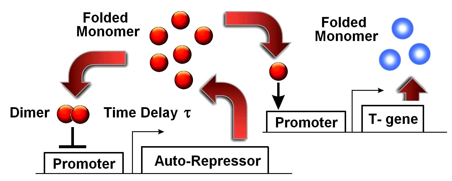
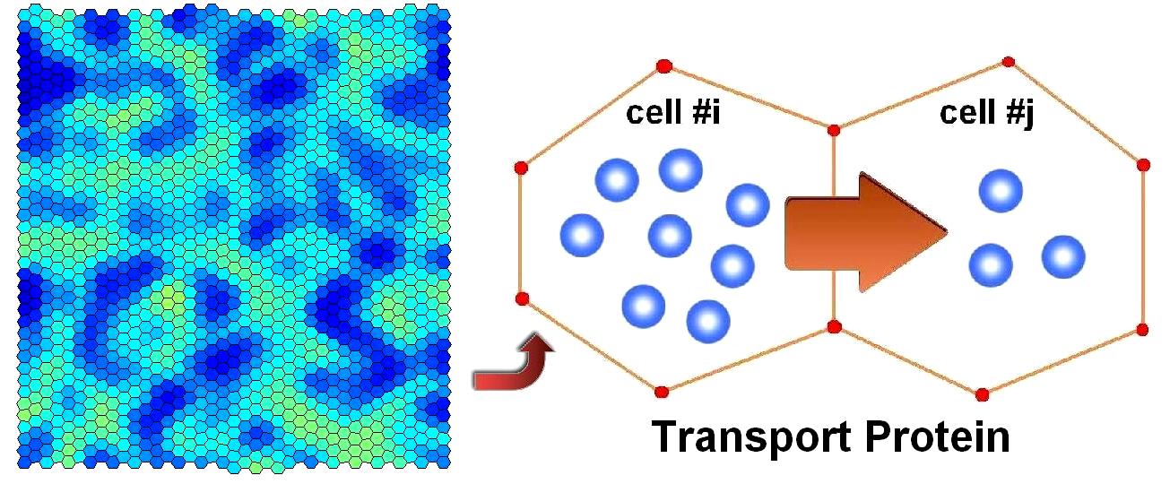
Figure 1: A single-gene autorepressor oscillator with a time-delayed negative feedback. Its protein (red circles) acts as a positive regulator of the transport protein (blue circles) by activating its transcription. The signaling species is diffused from one cell to the other within the lattice governed by the chemo-mechanical epithelium model described in pismen2 ; bratsun3 .

In this Letter, we explore the spatial effects produced by the combined action of the intrinsic noise and time delay within a multi-cellular system. It is based on the multi-scale chemo-mechanical model of the epithelial tissue which first was developed in pismen2 and then was applied to simulate the carcinoma growth bratsun3 . Using the lattice approach allows to avoid the problem of the lack of a reliable Gillespie-like algorithm for spatial non-Markovian processes and to apply the algorithm from bratsun1 . We use a single-gene auto-repressor model with constant delay at a single-cell level complemented by the dynamics of the transport species penetrating cell membranes (Fig. 1).

Epithelial tissue is a two-dimensional layer of cells covering the surface of an organ or body. The chemo-mechanical model includes the calculation of the dynamics of separate cells adapting to environmental stresses. The initial hexagonal lattice representing cells becomes distorted due to proliferation/intercalation and eventually incorporates also polygons with a different number of vertices. The epithelium is evolved by moving the cell nodes. The mechanical force acting on any $i$th node is defined via the elastic potential energy of the tissue pismen2 ; bratsun3 :

$${\bf F}_{i}=-\frac{1}{2}\frac{\partial}{\partial{\bf R}_{i}}\displaystyle\sum_{cells}\left(\kappa L^{2}+\eta(S-S_{0})^{2}\right)+{\bf F}^{st}_{i},$$ (1)

where ${\bf R}_{i}$ is the radious vector of $i$th node, $L$ and $S$ stand for the perimeter and area of a cell respectively. ${\bf F}^{st}_{i}$ is an uncorrelated zero mean stochastic input. The coefficient $\kappa$ defines the action of contractile forces within the cell cortex, $\eta$ reflects the cell resistance to any changes with respect to the reference area $S_{0}$.

Since the motion is strongly overdamped, the governing equation for the displacement should be written as

$$\frac{d{\bf R}_{i}}{dt}={\bf F}_{i}H\left(|{\bf F}_{i}|-F_{0}\right),$$ (2)

where $H$ is a Heaviside function, $F_{0}$ is the threshold force below which the node remains immobile. Altogether, Eqs. (1-2) define the mechanics of the tissue.

We consider a single-gene protein synthesis with negative auto-regulation (Fig. 1). This is a popular motif in genetic regulatory circuits, and its temporal dynamics has been analyzed within both deterministic and stochastic framework elston1 . This model is relatively simple yet but still maintains a high degree of biological relevance. Its generalized version accounting for the effect of time delay $\tau$ has been suggested in bratsun1 ; bratsun2 . Suppose that protein can exist both in the form of monomers X and dimers X_D. The transitions between them with the rates $k_{\pm d}$ are

$$\ce{X+X->[k_{+d}]X_{D}},\qquad\ce{X_{D}->[k_{-d}]X+X}.$$ (3)

We assume that the protein may be degraded with the rate $B$ and be produced with the rate $A$ respectively:

$$\ce{X->[B]\emptyset},\qquad\ce{D_{0}^{t}->[A]D_{0}^{t+\tau}+X^{t+\tau}}.$$ (4)

The synthesis occurs at time $t+\tau$ if the chemical state of the promoter site of the X gene at time $t$ is unoccupied (D₀). Otherwise (D₁), the production is blocked. The transitions between the states occur with rates $k_{\pm 1}$ during binding and unbinding of some dimer respectively

$$\ce{D_{0}+X_{D}->[k_{+1}]D_{1}},\qquad\ce{D_{1}->[k_{-1}]D_{0}+X_{D}}.$$ (5)

In order to describe the intercellular signaling, we introduce the transport species T positively regulated by the X protein (Fig. 1). If the operator site of the T gene is occupied (D${}_{1}^{T}$) then the T protein may be produced immediately with a certain probability $A_{T}$:

$$\ce{{\emptyset}->[A_{T}D^{T}_{1}(t)]T}.$$ (6)

If the site is unoccupied, the production of the T protein is blocked. Thus, the X monomers act as a positive regulator of T by activating its transcription, because the transitions between the states with the rates $k_{\pm 2}$ are

$$\ce{D_{0}^{T}+X->[k_{+2}]D_{1}^{T}},\qquad\ce{D_{1}^{T}->[k_{-2}]D_{0}^{T}+X}.$$ (7)

We assume also that once a signal has come in a certain cell, it is converted into the X monomers with the rate $B_{T}$ and the copy number $N$:

$$\ce{T->[B_{T}]X}.$$ (8)

Altogether, Eqs. (3-8) define the kinetics of gene regulation both at a single cell level and a whole tissue.

Figure 2: (a) Neutral curve of the Hopf bifurcation obtained within a single-cell deterministic description for $\varepsilon=0.1$, $\delta=0.2$. (b) Power spectrum obtained in a single-cell stochastic simulation below the Hopf bifurcation for $A=20$, $B=5$, $\tau=6$, $k_{+1}=100$, $k_{+d}=200$, $k_{-1}=1000$, $k_{-d}=1000$.

Deterministic description. The main approximation is that the reactions of dimerization (3) and binding/ unbinding (5,7) are fast in comparison with production/ degradation of proteins (4,6,8). Thus, their dynamics has to enter quickly into a local equilibrium and we arrive to

$$(1+4\varepsilon x_{i}){dx_{i}\over dt}=\frac{A}{1+\varepsilon\delta x_{i}^{2}(t-\tau)}+B_{T}\theta_{i}-Bx_{i},$$ (9)

$$\frac{d\theta_{i}}{dt}=\frac{NA_{T}\sigma x_{i}}{1+\sigma x_{i}}-B_{T}\theta_{i}+\displaystyle\sum_{j\in adj(i)}\alpha L_{ij}(\theta_{j}-\theta_{i}),$$ (10)

where the subscripts refer to cells, $x$ and $\theta$ stand for the concentrations of the X and T proteins respectively, $\alpha$ is the transfer coefficient, $\delta=k_{+d}/k_{-d}$, $\varepsilon=k_{+1}/k_{-1}$, $\sigma=k_{+2}/k_{-2}$ and $adj(i)$ stands for “adjacent to $i$-cell”. It is assumed that the T protein is transported diffusively from one cell to the other, whereas its flux does not depend on the distance between the two cells $i$ and $j$ but is proportional to the boundary length $L_{ij}$. This implies that the transport is limited by the transfer though cell membranes. The link between sub-cellular and macroscopic scales is established through the Eq. (10), since the $\theta$ field is global for the whole tissue (for more details, see Supplementary materials).

The neutral curve for the Hopf bifurcation derived within the deterministic approach (9-10) at a single-cell level is plotted in Fig. 2a in the plane of dimensionless parameters $\tau A$ and $\tau B$. The numerical study reveals the common dynamics below and above the bifurcation.

In order to study the spatial effects, the set of delay differential equations (9-10) has been solved using the explicit Euler method, whose stability was warranted by a sufficiently small time step. This procedure was synchronized with the simulation of the mechanical evolution governed by Eqs. (1-2). The initial configuration of the system is a hexagonal lattice comprising $1560$ cells with random phase distribution. The tissue as a whole has the form of a stripe. The typical values of the parameters governing the tissue mechanics hereinafter are as follows: $\kappa=1.0$, $\eta=1.0$, $S_{0}=3\sqrt{3}/2$, $F_{0}=0.02$. Fig. 3a presents the results of numerical simulation with parameters taken above the Hopf bifurcation curve (the upper black square in Fig. 2a). The X protein patterns are shown for two consecutive moments of time. The nonlinear dynamics includes the slow development of spiral traveling wave pattern which arises against the synchronized field oscillating in the background. The oscillation period is approximately equal to the triple delay time.

Stochastic description. In order to describe the spatial stochastic effects, we use a hybrid model, which is constructed as follows. The dynamics of the proteins in each cell has been obtained by performing direct stochastic simulations of the reactions (3-8) using the modified version of the Gillespie algorithm bratsun1 . The signaling between cells is still organized as diffusive transport from one cell to the other according to finite-difference formula:

$$T_{i}^{t+\triangle t}=T_{i}^{t}+\left[\triangle t\displaystyle\sum_{j\in adj(i)}\alpha L_{ij}(T_{j}^{t}-T_{i}^{t})\right],$$ (11)

where $[...]$ stands for the integer part of the expression. The time step in (11) is equal to the time step for the integration of (1-2): $\triangle t=0.05$. Since the typical time step stochastic system is much less ($\triangle t_{st}=0.00001-0.001$), one needs to dock the numerical schemes for the mechanical evolution of the tissue and stochastic fluctuations of the protein (see Supplementary materials).

(a)
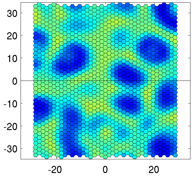
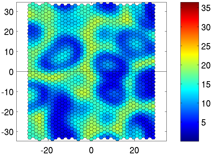
(b)

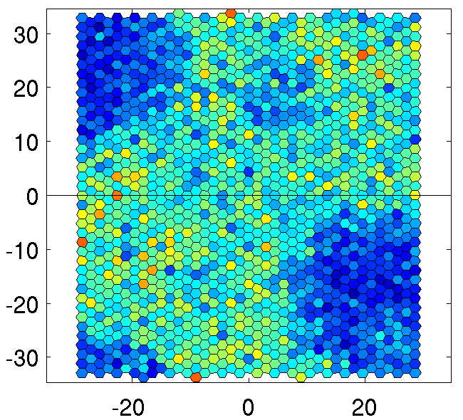
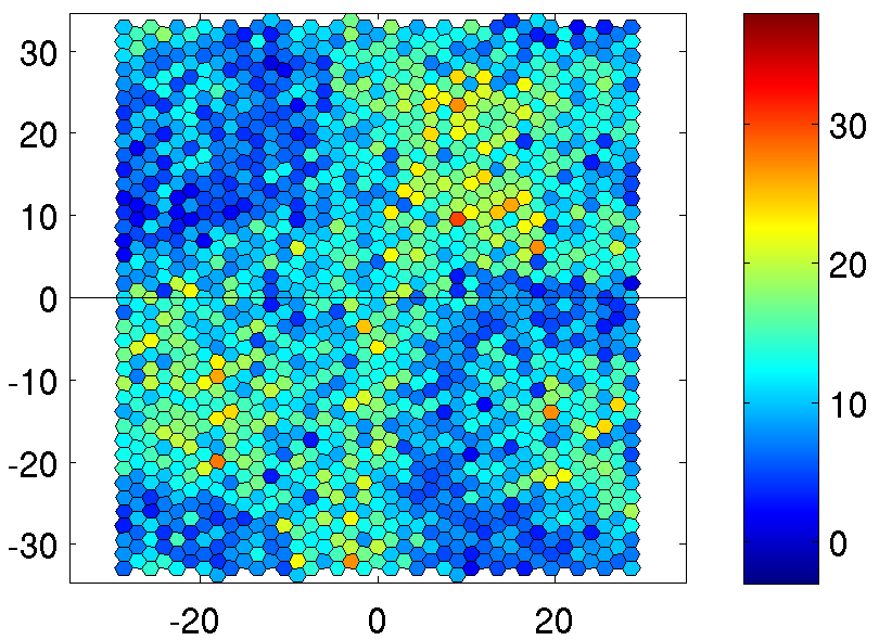
Figure 3: Evolution of the X protein pattern in the epithelium formed of more than 1500 cells within (a) deterministic and (b) stochastic description, with parameters $A=500$, $A_{T}=500$, $B=5$, $\tau=6$, $N=1$, $\alpha=0.05$, $k_{d}=200$, $k_{-i}=1000$, $k_{1,2}=100$ taken above deterministic Hopf bifurcation curve (see Fig. 2a). The frames correspond to times $t=260$, $340$.

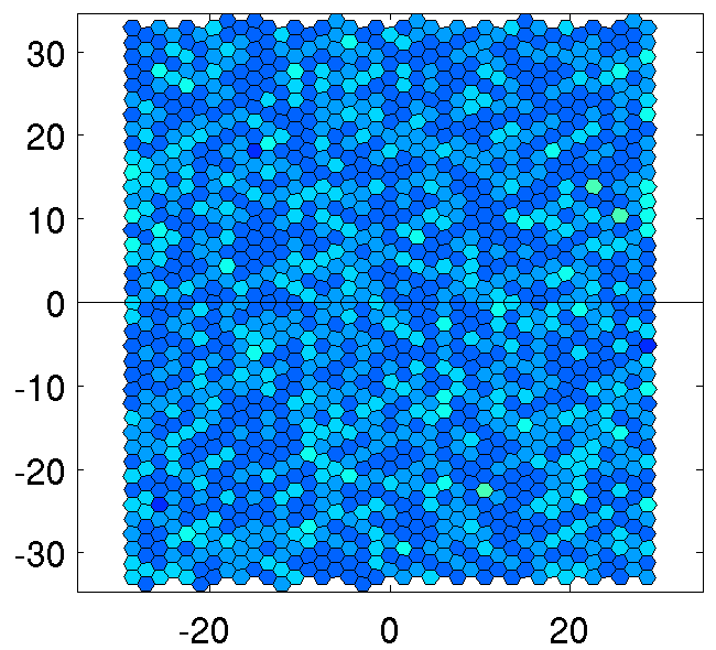
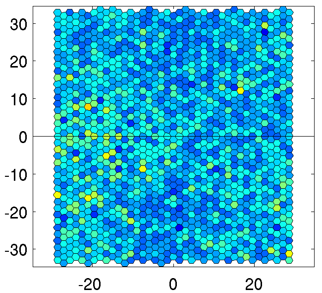
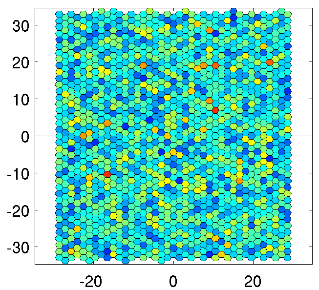
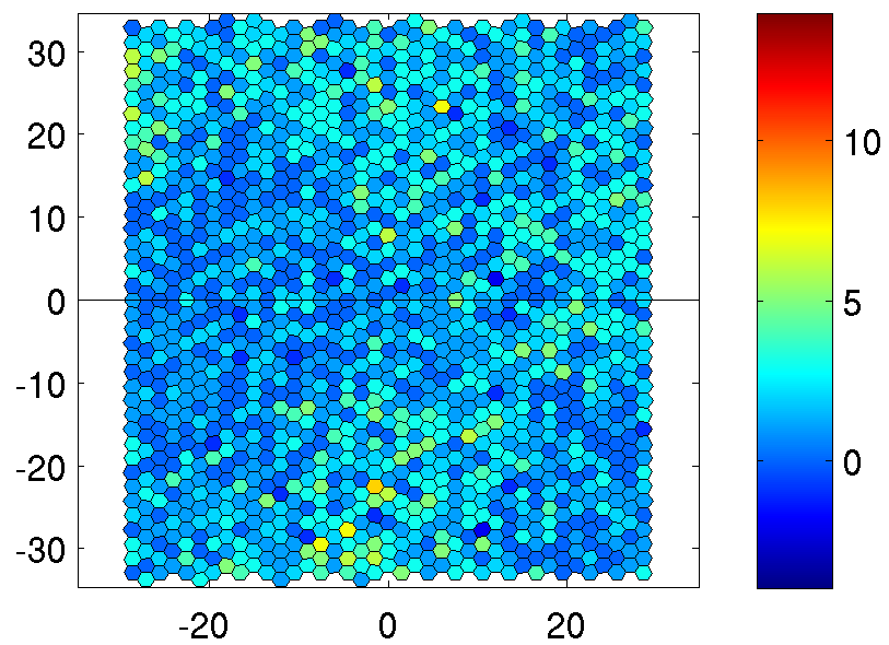
Figure 4: Stochastic pattern formation of the X protein in the epithelium far below the Hopf bifurcation (see Fig. 2a). The frames correspond to times within one oscillatory period $2\tau$. The parameters are the same as in Fig. 3, except $A=20$, $N=8$.

The power spectrum of time-delayed stochastic signal generated on a single-cell level far below the Hopf bifurcation is shown in Fig. 2b. It has a remarkable row of peaks indicating that some periodicity in the signal should exist. The first peak corresponds to the frequency $\omega^{*}=\pi/\tau\approx 0.524$ ($\tau=6$). One can observe also the strong harmonics of the fundamental frequency given by $\omega_{n}=(2n-1)\omega^{*}$. Thus, the time delay coupled with the noise can cause a system to be oscillatory even when its deterministic description predicts no oscillations.

Let us consider now two examples of spatial stochastic simulations. Fig. 3b presents the stochastic pattern formed by the X monomers in the tissue with the same parameter values as in Fig. 3a. We found that nonlinear dynamics of spatially extended system consists of two distinct oscillatory modes, just like it was in the deterministic case. One is a quasi-standing wave pattern oscillating with $\omega^{*}$. The second oscillatory mode consists of traveling waves which arise from selected initial disturbances. In fact, the stochastic pattern looks very similar to its deterministic counterpart obtained for the same parameters (compare with the upper row in the same figure). The wavelength of the structure is found to depend on the copy number $N$ whose growth enhances fluctuations and diffusive fluxes between cells.

Consider now the parameters taken far below the Hopf bifurcation curve (Fig. 2a). We found that starting with random initial conditions, the system fairly quickly falls into a fully synchronized mode of oscillations with a common frequency $\omega\approx\omega^{*}$ (Fig. 4, 5). We found also that the increase of the copy number $N$ can result in the clustering when the cells form two approximately equal communities, which oscillate in anti-phase. For instance, the numerical simulation with copy number $N=4$ has showed that the clustering is not observed. In contrast to that, this effect manifests itself clearly at $N=8$ after a sufficiently long integration (Fig. 4). In fact, the clustering in the system with a large amount of elements exchanging chemical signals has become at the center of attention of many scientists recently (see, for example, kos ). It is believed that the clustering is likely to be the reason of further cells differentiation in organs.

Closing remarks. It is known that the noise during gene expression comes about in two ways. The inherent stochasticity of transcription/translation generates intrinsic noise. The extrinsic noise refers to variation in identically-regulated quantities between different cells. In this paper, we have focused on spatial effects of intrinsic noise. A reliable Gillespie-like algorithm for the spatial non-Markovian systems still has not been developed, but perhaps, this algorithm is not very necessary. Since any living matter consists of cells, it is more practical to use numerical methods based on a computational mesh which represents a cellular compartment, such as a membrane or the interior of some part of a cell. In this paper, we have applied such lattice approach suggesting the model which includes both mechanical interactions and chemical signal exchanges between cells.

An important new result of this study is giving insight into how the excitation of quasi-regular delay-induced fluctuations found in bratsun1 , manifests itself in space. We show that above the Hopf bifurcation it is observed the traveling wave pattern which is similar to that in the deterministic case. But more interesting result is found below the Hopf bifurcation where the deterministic system is stable: there may be observed both a spatial synchronization of oscillations and clustering of cell community.

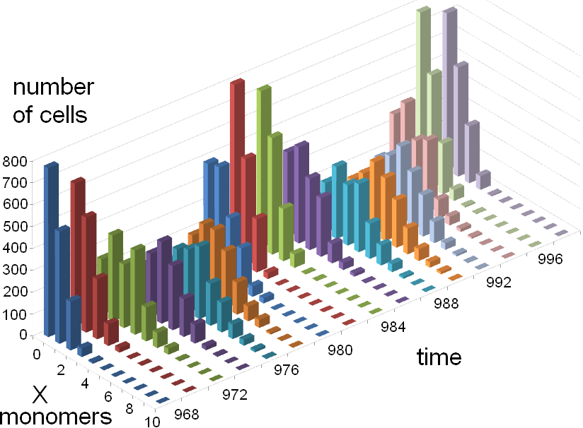
Figure 5: Time evolution of the distribution of stochastic oscillation phases in cells obtained far below deterministic Hopf bifurcation. Two periods of spatially synchronized oscillations are shown. The parameters are the same as in Fig. 4.

We wish to thank L.M. Pismen for stimulating discussions. The work was supported by the Perm Ministry of Education and RFBR (grant 14-01-96022r_ural_a).

References

- (1) T. B. Kepler, T. C. Elston, Biophys. J. 81, 3116 (2001).
- (2) M. Kaern, T. C. Elston, W. J. Blake and J. J. Collins, Nat. Rev. Genet. 6, 451 (2005).
- (3) N. Rosenfeld, J. W. Young, U. Alon, P. S. Swain and M. B. Elowitz, Science. 307, 1962 (2005).
- (4) D. J. Wilkinson, Nat. Rev. Genet. 10, 122 (2009).
- (5) L. S. Tsimring, Rep. Prog. Phys. 77, 026601 (2014).
- (6) D. Bratsun, D. Volfson, J. Hasty, and L. Tsimring, Proc. SPIE 5845, 210 (2005).
- (7) D. Bratsun, D. Volfson, J. Hasty and L.S. Tsimring, Proc. Natl. Acad. Sci. U.S.A. 102, 14593 (2005).
- (8) J. L. Doob, Trans. Amer. Math. Soc. 52, 37 (1942).
- (9) D. T. Gillespie, J. Phys. Chem. 81, 2340 (1977).
- (10) D. J. Higham, SIAM Rev. 50, 347 (2008).
- (11) J. Pahle, Brief Bioinform 10, 53 (2009).
- (12) T. Székely and K. Burrage, Comput. Struct. Biotechnol. J. 12, 14 (2014).
- (13) C. Lemerle, B. di Ventura and L. Serrano, FEBS Letters. 579, 1789 (2005).
- (14) C.-W. Li and B.-S. Chen, Gene Regulation and Systems Biology. 3, 191 (2009).
- (15) K. Burrage, P. M. Burrage, A. Leier, T. Marquez-Lago and D. V. Nicolau, in Design and Analysis of Biomolecular Circuits: Engineering Approaches to Systems and Synthetic Biology edited by H. Koeppl et al., Stochastic Simulation for Spatial Modelling of Dynamic Processes in a Living Cell, 43 (Springer, Heidelberg, 2011).
- (16) D. V. Nicolau and K. Burrage, Comput. Math. Appl. 55, 1007 (2008)
- (17) T. T. Marquez-Lago, A. Leier and K. Burrage, BMC Syst. Biol. 4, 19 (2010).
- (18) T. Danino, O. Mondragon-Palomino, L. Tsimring and J. Hasty, Nature 423, 326 (2010).
- (19) M. Salm and L.M. Pismen, Phys. Biol. 9, 026009 (2012).
- (20) D. Bratsun, A. Zakharov and L. Pismen, in Emergence, Complexity and Computation, edited by A. Sanayei et al., Modeling of Tumour Growth Induced by Circadian Rhythm Disruption in Epithelial Tissue, Vol. 14, 295 (Springer, Heidelberg, 2015).
- (21) A. Koseska, E. Ullner, E. Volkov, J. Kurths, J. Garcia-Ojalvo, J. Theor. Biol. 263, 189 (2010).