Effects of a dressed quark-gluon vertex in pseudoscalar heavy-light mesons

Abstract

Using a simple model in the context of the Dyson-Schwinger-Bethe-Salpeter approach, we investigate the effects of a dressed-quark-gluon vertex on pseudoscalar meson masses. In particular, we focus on the unequal-mass case and investigate heavy-light meson masses; in addition, we study the premise of the effective treatment of heavy quarks in our approach.

I Introduction

The realm of heavy-light mesons is topical and promising for a number of reasons. In the light of quantum chromodynamics (QCD), one faces the challenge of a multi-scale problem, where many successful theoretical Ansätze can be tested, compared, and brought together. With the chiral limit on one and the heavy-quark regime on the other end of the quark mass range, an ideal approach should respect the symmetries apparent in QCD at both of these ends together with the other basic properties of the theory, e. g., its perturbative limit, and a realization of confinement. Overall, a nonperturbative technique is necessary and has the benefits of wide applicability, if used properly and with a model tailored to this task.

In particular, it has been shown in Hilger and Kämpfer (2009); Hilger et al. (2010, 2012a, 2011, 2012b); Buchheim et al. (2014) that the spectral difference of parity partners in the sector of mesons with a heavy and a light valence quark is driven by a subtle balance between a suppressed interaction with the QCD ground state and an enhanced impact of light-quark chiral-symmetry breaking effects by the heavy-quark mass. The mass splitting of these parity partners is comparable to the ones in the sector of mesons with light valence quarks only, making them a suitable object for related investigations of dynamical chiral-symmetry breaking.

The Dyson-Schwinger-Bethe-Salpeter-equation (DSBSE) approach, a modern nonperturbative tool for quantum field theory Roberts et al. (2007); Fischer (2006); Alkofer and von Smekal (2001); Sanchis-Alepuz and Williams (2015a) complementary to the well-known lattice-regularized approach Dudek et al. (2008); Liu et al. (2012); Thomas (2013); Flynn et al. (2015), is an excellent candidate for such a study, since all requirements are met. In this work we build on an earlier investigation of a systematic approach to dressing the quark-gluon vertex (QGV) and thus, consistently the quark Dyson-Schwinger-equation (DSE) and meson Bethe-Salpeter-equation (BSE) integration-equation kernels Bhagwat et al. (2004); Gomez-Rocha et al. (2014), which are the necessary prerequisites for a meson study. Vertex dressing affects the BSE kernel in the various mesonic $J^{PC}$ channels differently, which is in accord with expectations from the quark model, where different terms in the potential also show varying importance in different channels, see, e. g., Godfrey and Isgur (1985).

In modern DSBSE studies with sophisticated effective interactions, a simple truncation offers the possibilities of comprehensive investigations, see Maris and Tandy (1999); Holl et al. (2004, 2005a); Krassnigg (2009); Krassnigg and Blank (2011); Dorkin et al. (2011); Mader et al. (2011); Hilger (2012); Popovici et al. (2014); Hilger et al. (2015a); Fischer et al. (2014, 2015); Hilger et al. (2015b) and references therein. Beyond the most popular rainbow-ladder (RL) truncation, there have also been sophisticated studies, following systematic schemata based on the structure of the DSE tower. However, the numerical effort Bhagwat et al. (2007a); Krassnigg (2008); Blank and Krassnigg (2011a, b); Blank (2011) quickly increases Watson and Cassing (2004); Watson et al. (2004); Fischer et al. (2005); Fischer and Williams (2008, 2009); Williams (2010, 2015); Sanchis-Alepuz et al. (2014); Chang and Roberts (2009); Heupel et al. (2014); Sanchis-Alepuz and Williams (2015b) and so there have been a number of investigations, like our present one, which make use of a very simple effective interaction Munczek and Nemirovsky (1983) in order to be able to highlight particular schemes or effects, if one is able to sum up certain classes of diagrams or study a certain scheme in as great detail as possible Bender et al. (1996); Alkofer and von Smekal (2001); Bender et al. (2002); Krassnigg and Roberts (2004); Bhagwat et al. (2004); Holl et al. (2005b); Matevosyan et al. (2007a, b); Jinno et al. (2015). Apart from elucidating effects of high-order dressing terms or fully summed subclasses of diagrams, such studies provide a guide as to how far a systematic truncation scheme with a sophisticated effective interaction would have to go in order to achieve reliable results for various hadron properties.

Our focus on heavy-light meson systems can help to study the importance of QGV correction terms by testing those in a multiply unbalanced system of one light (and at the same time very strongly-dressed) antiquark together with one heavy (and only mildly-dressed) quark in a relativistic bound state. Note that investigations of heavy-quark propagators have shown that dressing can have sizeable effects even for the case of b-quarks Nguyen et al. (2009); Souchlas and Stratakis (2010); Nguyen et al. (2011). In contrast to earlier DSBSE studies making use of particular assumptions about heavy-quark propagators Ivanov et al. (1998a, b, 1999); Blaschke et al. (2000); Bhagwat et al. (2007b); Ivanov et al. (2007); El-Bennich et al. (2010, 2011) we would like to motivate or justify these assumptions rather than start out from them. Ultimately, we aim at a direct check of heavy-quark symmetry predictions Neubert (1994) like the ones performed recently, e. g., in relativistic Hamiltonian dynamics Gomez-Rocha and Schweiger (2012).

The article is organized as follows: In Sec. II we present the setup used for the quark DSE, the QGV, and the meson BSE. Results are collected and discussed in Sec. III for both the quark propagator dressing functions and the meson masses. After the conclusions in Sec. IV we have collected more technical details and explanations as well as a complete set of results in terms of tables and figures together with an analysis of heavy-quark effective quark propagators and their comparison to the ones computed here in several appendices.

II Setup

Since this work is an extension of Bender et al. (2002); Bhagwat et al. (2004), we focus on essentials and differences instead of repeating every detail here. Our calculations are performed in Euclidean space.

II.1 Quark DSE

For the purpose of investigating hadrons as bound states of (anti)quarks interacting via gluons, the DSE for the quark propagator is an adequate starting point, because it contains two main ingredients of such a study, namely the renormalized dressed gluon propagator $D_{\mu\nu}$ and the renormalized dressed QGV $\Gamma^{a}_{\nu}$ with the color index ^a. Its solution is the renomalized dressed quark propagator $S$ for a particular quark flavor, which has the general structure

$$S(p)^{-1} = i\gamma\cdot pA(p^{2})+B(p^{2})$$ (1)

$$= A(p^{2})\left(i\gamma\cdot p+M(p^{2})\right)\;.$$ (2)

In this and the following, we omit dependences on renormalization and regularization parameters and details due to the particular ultraviolet-finite model interaction we are using herein: the corresponding renormalization constants are $=1$.

The dressing functions $A$ and $B$ characterize $S$ completely. Alternatively, one can use $A$ and $M$, all of which are functions of the quark momentum $p$ squared, and implicitly also of the current-quark mass $m_{q}$ and thus the quark’s flavor. We write $s:=p^{2}$ and choose to investigate $A(s)$ and $M(s)$ below.

The quark DSE reads

$$S^{-1}(p) = S^{-1}_{0}+\Sigma(p)=i\gamma\cdot p+m_{q}+\Sigma(p)$$ (3)

$$= S^{-1}_{0}+\int_{q}\!\!g^{2}D_{\mu\nu}(p-q)\frac{\lambda^{a}}{2}\gamma_{\mu}S(q)\Gamma^{a}_{\nu}(q;p)$$ (4)

with $\int_{q}:=\int\frac{d^{4}q}{(2\pi)^{4}}$, $\Sigma$ the quark self energy, $p$ the quark momentum, and $g$ the strong coupling constant. The subscript ₀ denotes a bare quantity. With the specification of the effective interaction with constant strength $\mathcal{G}$ to be used herein Munczek and Nemirovsky (1983) via

$$g^{2}\,D_{\mu\nu}(k):=\left(\delta_{\mu\nu}-\frac{k_{\mu}k_{\nu}}{k^{2}}\right)(2\pi)^{4}\,\mathcal{G}^{2}\,\delta^{4}(k)\,,$$ (5)

one arrives at an algebraic equation for $S$; the same is also true for the other equations of relevance herein, namely the DSE for the QGV and the meson BSE. More precisely, with the explicit color prescription $\Gamma_{\mu}^{a}(p)=\frac{\lambda^{a}}{2}\Gamma_{\mu}(p)$ and setting $\mathcal{G}=1$, thereby obtaining all dimensioned quantities in appropriate units of $\mathcal{G}$ one obtains

$$S^{-1}(p)=i\gamma\cdot p+m_{q}+\gamma_{\mu}S(p)\Gamma_{\nu}^{\mathcal{C}}(p)\;,$$ (6)

where the model parameter $\mathcal{C}$ introduced at this point is defined below. At this point the quark DSE can be solved for any explicit form of the QGV, and results in physical units are obtained by providing the necessary input, i. e., a value for the model strength parameter $\mathcal{G}$ and a quark mass $m_{q}$ for any given quark flavor.

To proceed, one can make use of the DSE for the QGV in order to define a model for $\Gamma_{\nu}^{\mathcal{C}}(p)$. In particular, again following Bhagwat et al. (2004), the QGV DSE is used to obtain the effective equation

$$\Gamma_{\mu}^{\mathcal{C}}(p)=\gamma_{\mu}-\mathcal{C}\,\gamma_{\rho}\,S(p)\,\Gamma_{\mu}^{\mathcal{C}}(p)\,S(p)\,\gamma_{\rho}\;,$$ (7)

whose dependence on $\mathcal{C}$ stems from the effective combination of the abelian and non-abelian correction terms in the QGV DSE such that: i) any differences in strength or momentum dependence of these two terms is taken to be proportional to the simple and herein accessible structure of the abelian term; ii) the sign is that of the non-abelian correction due to its dominant role; and iii) $\mathcal{C}$ is chosen in accordance with either lattice QCD, phenomenology, or another reasonable point of comparison.

From a general point of view, the following values are of interest: $\mathcal{C}=-1/8$ corresponds to the case with abelian-only dressing as, e. g., used in Bender et al. (2002). $\mathcal{C}=0$ corresponds to the popular RL truncation, which is also the zeroth order in the systematic schemes of the kind considered here. Finally, $\mathcal{C}=0.51$ was used in Bhagwat et al. (2004) as a result from fitting to lattice quark propagators, with good phenomenological success. We fix $\mathcal{C}=0.51$ throughout herein in order to avoid the overwhelming amounts of data that would result from a thorough investigation of variation in all available parameters. For our purposes it is best to continue from Bhagwat et al. (2004) for clarity of the resulting effects, easy comparison, and direct applicability.

Equation (7) is the immediate basis for an iterative prescription, where the bare QGV serves as a starting value: $\Gamma_{\mu,0}^{\mathcal{C}}(p)=\gamma_{\mu}$. The recursion relation is

$$\Gamma_{\mu,i}^{\mathcal{C}}(p)=-\mathcal{C}\,\gamma_{\rho}\,S(p)\,\Gamma_{\mu,i-1}^{\mathcal{C}}(p)\,S(p)\,\gamma_{\rho}$$ (8)

so that at a given order $n$ in this scheme one has for the QGV

$$\Gamma_{\mu}^{\mathcal{C}}(p)=\sum_{i=0}^{n}\Gamma_{\mu,i}^{\mathcal{C}}(p).$$ (9)

and the final result for the QGV is obtained by $n\rightarrow\infty$.

At this point it is also important to note that, like the solution of the quark DSE, also the corresponding result for the QGV implicitly depends on the flavor (and $m_{q}$) of the quark it is associated with, i. e., the details and properties of the factors $S(p)$ in Eqs. (7) and (8). Note also that, since the quark-gluon interaction is not flavor changing, both factors $S(p)$ in each of these equations must correspond to the same flavor and value of $m_{q}$.

II.2 Meson BSE

The meson BSE reads

$$[\Gamma(P;k)]_{EF}=\int_{q}[K(P;k;q)]_{EF}^{GH}[S(q_{+})\,\Gamma(P;q)\,S(q_{-})]_{GH}$$ (10)

where the four-vector arguments $P$ and $k$, $q$ are the quark-antiquark pair’s total and relative momenta, respectively. $E,F,G,H$ stand for color, flavor and spinor indices, $\Gamma(P;q)$ is the meson’s Bethe-Salpeter amplitude (BSA), and $K$ the fully-amputated dressed-quark-antiquark scattering kernel. The combination of quark propagators and the BSA is often combined to the so-called Bethe-Salpeter wave function $\chi$ and one writes

$$\chi(P;q):=S(q_{+})\,\Gamma(P;q)\,S(q_{-})\;,$$ (11)

where the meson flavor is determined by the combination of quark flavors from the two factors of $S$. The quark and antiquark momenta are defined as $q_{+}=q+\eta P$ and $q_{-}=q-(1-\eta)P$. $\eta$ is called the momentum partitioning parameter, and its arbitrariness in any computation is equivalent to the freedom in the definition of the quark-antiquark relative momentum. In a covariant setup, any observable should be independent of $\eta$; still, numerical approximations, truncations, or other model defects can destroy this independence, as is the case here, where the BSA is incomplete due to the particular form of the model interaction in Eq. (5). As a result, any study using this particular interaction should investigate also the $\eta$-dependence of numerical results; such an analysis was also performed in Ref. Munczek and Nemirovsky (1983) where this particular form of effective interaction was introduced in RL truncation. Still, such a model artifact does not destroy the model’s capacity to elucidate our targeted meson properties and can be easily quantified; thus it is well under control.

Provided one has solutions of the quark DSE for a given form of the quark self-energy $\Sigma$, taking into account a particular form $\Gamma_{\nu}$ of the QGV, one can construct a BSE interaction kernel consistent with the quark propagator dressing functions via the axial-vector Ward-Takahashi identity (AVWTI) Munczek (1995); Maris and Roberts (1997). It was shown in Bender et al. (1996, 2002); Bhagwat et al. (2004) that the BSE kernel corresponding to our particular setup when omitting contributions from gluon-unquenching Watson and Cassing (2004); Fischer et al. (2005) for equal-mass constituents in the BSE reads

$$\Gamma^{M}(P;k) = -\frac{4}{3}\int_{q}D_{\mu\nu}(k-q)\left[\gamma_{\mu}\chi^{M}(P;q)\,\Gamma_{\nu}(q_{-},k_{-})\right.$$ (12)

$$+ \left.\gamma_{\mu}S(q_{+})\,\Lambda^{M}_{\nu}(P;k;q)\right]\;.$$

The color trace has been carried out at this point, since the mesonic case is straight-forward in this regard; in the following, we always give results with evaluated color traces. The superscript label ^M denotes applicability to a particular meson, e. g., a pseudoscalar, which we investigate herein. This is important, because the structure of the correction term $\Lambda^{M}_{\nu}$ crucially depends on the structure of the corresponding BSA. We will detail this point below for the pseudoscalar case.

While the first term on the r.h.s. of Eq. (12) is constructed immediately from the given QGV, the construction of the second term is again based on a recursion relation analogous to the one for the QGV. One sums up the correction terms up to a particular order $n$ to get $\Lambda^{M}$:

$$\Lambda^{M}_{\nu}(P;k;q)=\sum_{i=0}^{n}\Lambda_{\nu,i}^{M}(P;k;q)\,.$$ (13)

The full result is then obtained by $n\rightarrow\infty$.

Generalizing to the unequal-mass case, we symmetrize Eq. (12) to get

$$\Gamma^{M}(P;k) = -\frac{1}{2}\frac{4}{3}\int_{q}D_{\mu\nu}(k-q)\left[\gamma_{\mu}\chi^{M}(P;q)\,\Gamma_{\nu}(q_{-},k_{-})\right.$$ (14)

$$+ \gamma_{\mu}S(q_{+})\,\Lambda^{M}_{\nu}(P;k;q)+\Gamma_{\mu}(q_{+},k_{+})\chi^{M}(P;q)\gamma_{\nu}$$

$$+ \left.\Lambda^{M}_{\mu}(P;k;q)S(q_{-})\gamma_{\nu}\right]\;.$$

The flavor content of this equation is encoded via the quark propagators and, more precisely, their arguments, the quark momenta $k_{\pm},q_{\pm}$: any factor of $S$ or $\Gamma_{\nu}$ with (an) argument(s) with subscript ₊ corresponds to the quark $1$ with flavor $1$ and those with (an) argument(s) with subscript _- corresponds to the antiquark $2$ with flavor $2$. We note here also that in our setup for unequal quark masses, the heavier one is associated with the subscript ₊.

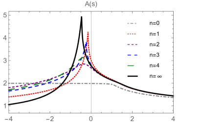
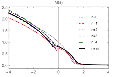
Figure 1: Dressing functions $A(s)$ and $M(s)$ for different values of $n$, corresponding to a quark mass $m_{u}=0.01$GeV.

The situation becomes clearer, when we employ the effective interaction from Eq. (5) to get the algebraic form

$$\Gamma^{M}(P;k) = -\frac{1}{2}\left[\gamma_{\mu}\chi^{M}(P;k)\,\Gamma_{\nu}^{\mathcal{C}}(k_{-})\right.$$ (15)

$$+ \gamma_{\mu}S(k_{+})\,\Lambda^{M}_{\nu}(P;k)+\Gamma_{\mu}^{\mathcal{C}}(k_{+})\chi^{M}(P;k)\gamma_{\nu}$$

$$+ \left.\Lambda^{M}_{\mu}(P;k)S(k_{-})\gamma_{\nu}\right]\;,$$

where we have written $\Lambda^{M}_{\nu}(P;k):=\Lambda^{M}_{\nu}(P;k;k)$ and denote the dependence on the parameter $\mathcal{C}$ explicitly.

One thus finds Bender et al. (2002); Bhagwat et al. (2004):

$$\frac{1}{\mathcal{C}}\Lambda_{\nu,n}^{M}(P;k) = -\gamma_{\rho}\chi^{M}(P;k)\Gamma_{\nu,n-1}^{\mathcal{C}}(k_{-})S(k_{-})\gamma_{\rho}$$ (16)

$$- \gamma_{\rho}S(k_{+})\Gamma_{\nu,n-1}^{\mathcal{C}}(k_{+})\chi^{M}(P;k)\gamma_{\rho}$$

$$- \gamma_{\rho}S(k_{+})\Lambda_{\nu,n-1}^{M}(P;k)S(k_{-})\gamma_{\rho}\;,$$

where one has to take care of attributing the correct quark flavors and factors of $S$ and $\Gamma_{\nu}$ according to their arguments with respect to the subscripts _±, as described above. This expression can be computed, the recursive terms for $\Lambda_{\nu,i}^{M}(P;k)$ summed up to any desired order, and the resulting algebraic equations can be solved. It is helpful to note here that also for $n\rightarrow\infty$ the equations can be solved explicitly via geometric summation.

The initial condition for this recursion relation is Bender et al. (2002)

$$\Lambda_{\nu,0}^{M}(P;k)=0\;,$$ (17)

which (only) in the pseudoscalar case for equal-mass quarks and $\eta=1/2$ implies Bender et al. (2002)

$$\Lambda_{\nu,0}^{PS}(P;k)=0\quad\Rightarrow\quad\Lambda_{\nu}^{PS}(P;k)\equiv 0\;,$$ (18)

which is an excellent testing case for our general setup. Further details on this construction are rather technical and are thus collected in App. D.

III Results and Discussion

In the present investigation we ask the question how important corrections to the popular RL truncation are in the case of mesons with unequal-mass constituents. While our results allow not only qualitative, but also quantitative statements, caveats are due to the simplicity of the interaction and the resulting oversimplification of structures related to relative quark-antiquark momentum, as well as the resulting artificial dependence on the momentum-partitioning parameter $\eta$. As a result, we not only attempt to study and quantify effects related to the number of recursion steps used for the QGV and the BSE kernel, which is our main objective, but also investigate the dependence of relevant quantities on $\eta$. The subsection on the quark DSE results, however, is independent of $\eta$.

Our model parameters are fixed to: $\mathcal{C}=0.51$ sets the amount and quality of dressing in the DSE of the QGV, and is fixed throughout this paper, as mentioned above. Investigations of the effect of using different values of $\mathcal{C}$ have been performed in Bhagwat et al. (2004) for equal-mass constituents to some extent, but mainly concerning the change from the abelian value of $\mathcal{C}=-1/8$ to a non-abelian-dominated version, which is phenomenologically reasonable and extendable. A detailed investigation of the $\mathcal{C}$-dependence of our results is beyond the present study and thus deferred to subsequent publications.

The effective coupling is set to $\mathcal{G}=0.69$, a value compatible and preadjusted to fit vector-meson masses throughout entire quark-mass range. This fact also explains why our results for pseudoscalar mesons as they are presented below in Fig. 5 do not appear completely satisfactorily on the level of a pure theory-experiment comparison. This is, however, not the main point of our study and serves mainly to keep all masses and quantities under investigation on their respective domains of reasonable values.

Finally, we also take the current-quark masses directly from Bhagwat et al. (2004) and set $m_{u}=0.01$GeV, $m_{s}=0.166$GeV, $m_{c}=1.33$GeV, $m_{b}=4.62$GeV. For the pion we assume isospin symmetry and the equality of the current-quark masses of the $u$ and $d$ quarks.

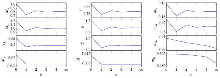
Figure 2: $n$-dependence of various quantities: dressing functions $M(s)$ and meson masses, all in GeV. Left panel: $M(s=0)$ for all four quark masses; center panel: Calculated mass function $M(s)$ at $s=-m_{H}^{2}/4$. For the unequal-mass case the mass function of the heavier quark is presented. The experimental values are used for the meson masses $m_{H}$ (see text). The labels $H$ of the subplots denote $\pi$, $K$, $D$, $B$; right panel: Pseudoscalar bound-state masses for the equal-mass case calculated from the BSE for different quark flavors.

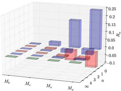
Figure 3: Relative differences $R_{n}$ of dressing functions $M(0)$ for $n$ loops compared to the case $n\rightarrow\infty$, for all four quark masses.

III.1 Quark DSE

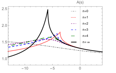
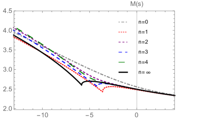
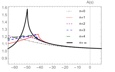
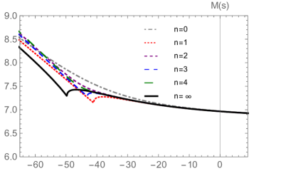
Figure 6: Quark propagator dressing functions $A(s)$ and $M(s)$ as functions of $n$, where $n=0$ and $n=\infty$ are represented by the dashed and thick solid lines, respectively. Upper left and right panels: $A(s)$ and $M(s)$ for $m_{s}=0.166$GeV; middle left and right panels: $A(s)$ and $M(s)$ for $m_{c}=1.33$GeV; lower left and right panels: $A(s)$ and $M(s)$ for $m_{b}=4.62$GeV.

The equations resulting from the general setup described in Sec. II, after applying the effective interaction defined in Eq. (5), are algebraic and can be tackled via standard root-finding techniques. We note here that the solutions from equations involving polynomials can be defined piecewise, as is also the case in our investigation and visible in Figs. 1 and 6.

A typical set of solutions for the dressing functions $A(s)$ and $M(s)$ is plotted in Fig. 1 for the light quark mass and different

Table 1: Calculated mass function $M(s)$ at $s=0$ for light and heavy quarks, in GeV.

	$M_{u}(s=0)$	$M_{s}(s=0)$	$M_{c}(s=0)$	$M_{b}(s=0)$
$n=0$	1.011	1.182	2.556	6.972
$n=1$	0.731	0.941	2.481	6.966
$n=2$	0.837	1.027	2.497	6.966
$n=3$	0.798	0.998	2.494	6.966
$n=4$	0.814	1.009	2.494	6.966
$n=\infty$	0.810	1.006	2.494	6.966

steps in the recursion, starting from $n=0$, which corresponds to RL truncation, and including the fully dressed vertex represented by $n=\infty$. Analogous plots for the strange, charm, and bottom masses can be found in Fig. 6 in App. A.

It is notable, how the simple behaviour of $A$ and $M$ are changed from the RL result (dashed lines) with the QGV dressing switched on. The change is more drastic for $A$, where one can find qualitatively different trends on the timelike domain at the scales relevant for the respective bound states, i. e., $s=-m_{M}^{2}/4$, where $m_{M}$ is the bound state’s mass. For $M$ the changes are less pronounced; however they are certainly quantitatively relevant. In addition, $M$ appears together with $A$ in the denominator of the dressed propagators, where their effects are combined.

To illustrate this further, we present both tabulated concrete values as well as plots. First of all, we tabulate the mass function $M(s)$ at $s=0$, which is one possible definition of a constituent-quark mass, in Tab. 1. The same information is plotted in the left panel of Fig. 2. One observes two main features: First, the results seem to alternate in the sign of the effect relative to the fully dressed result with respect to $n$: odd $n$ yields a lower result than $n\rightarrow\infty$, even $n$ a higher one. Secondly, as expected, dressing effects are weaker in the heavy-quark domain. While the changes are pronounced in the light-quark case, a result identical to the one for $n\rightarrow\infty$ is reached already for $n=3$ for the charm quark, and $n=1$ for the bottom quark, respectively. Defining the relative changes from RL truncation ($n=0$) to the fully dressed result ($n\rightarrow\infty$) as

$$R_{n}:=\frac{M_{n}(s=0)-M_{\infty}(s=0)}{M_{\infty}(s=0)}\;,$$ (19)

we obtain $R_{0}$-values of $0.25$ for the $u$ quark, $0.17$ for the $s$ quark, $0.025$ for the $c$ quark, and $0.00086$ for the $b$ quark. This comparison, together with values of $R_{n}$ for all $n$ and quark masses are plotted in Fig. 3.

Table 2: Calculated mass function $M(s)$ at $s=-m_{H}^{2}/4$, in GeV. For the unequal-mass case the mass function of the heavier quark is presented. The experimental values are used for the meson masses $m_{H}$ (see text).

$H$	$\pi$	$K$	$D$	$B$	$\eta_{c}$	$\eta_{b}$
$n=0$	1.014	1.204	2.620	7.013	2.733	7.157
$n=1$	0.731	0.943	2.516	7.004	2.559	7.123
$n=2$	0.839	1.041	2.540	7.004	2.613	7.126
$n=3$	0.799	1.005	2.535	7.004	2.598	7.126
$n=4$	0.815	1.019	2.536	7.004	2.603	7.126
$n=\infty$	0.811	1.015	2.536	7.004	2.602	7.126

In a similar fashion, we present values for the mass functions for different quarks at that value of $s$ which appears as the argument of the dressing functions of $S$ in the solution of the BSE. For the case of the effective interaction (5) used herein this is proportional to $\eta^{2}$ and the pseudoscalar bound-state mass-squared. While we investigate the entire range of values of $\eta$ from $0$ to $1$ below, we use $\eta=0.5$ for the purpose of this argument and set $s=-m_{H}^{2}/4$. The corresponding numbers are collected in Tab. 2 and the first four columns are also plotted in the center panel of Fig. 2. For the unequal-quark-mass case we give/plot values of the mass function corresponding to the heavier quark flavor. In order to avoid additional uncertainty, the experimental values are used for the meson masses $m_{H}$ for each meson as given in the column labels: $m_{\pi}=0.140$ GeV, $m_{K}=0.494$ GeV, $m_{D}=1.870$ GeV, $m_{B}=5.279$ GeV, $m_{\eta_{c}}=2.984$ GeV, and $m_{\eta_{b}}=9.398$ GeV. It should be noted here that in the heavy-light case with values of $\eta$ ranging from $0$ to $1$ one potentially covers the whole range $s=-m_{H}^{2}$ to $s=0$, corresponding to $\eta=1$ and $\eta=0$, respectively. This is particularly interesting regarding the behavior of the dressing functions with $n$ as discussed in more detail in App. A

The pattern in Tabs. 1 and 2 are similar, which confirms a consistent picture of the dressing effects on the functions $A(s)$ and $M(s)$ on the entire relevant parts of the timelike $s$ domain. This remark remains also valid if one uses a more sophisticated effective interaction than the one of Eq. (5): in such a case, the integral-equation character of the BSE remains intact and the domain on which $A(s)$ and $M(s)$ are sampled most prominently in the complex $s$ plane is the one surrounding the negative real axis, reaching out to a scale of $s=-m_{H}^{2}/4$; for more details, see the appendices of Krassnigg and Blank (2011); Blank and Krassnigg (2011c); Dorkin et al. (2014); Hilger et al. (2015a); Dorkin et al. (2015).

It is illustrative to note here that the alternating convergence pattern between even and odd $n$ can be attributed to the negative sign of the r.h.s. of Eq. (8), the recursion relation for the QGV.

III.2 BSE

Table 3: Pseudoscalar bound-state masses for equal quark masses calculated from the BSE for different quark masses, in GeV.

	$\pi$	$0^{-+}_{\bar{s}s}$	$\eta_{c}$	$\eta_{b}$
$n=0$	0.149	0.669	3.033	9.505
$n=1$	0.132	0.604	…	…
$n=2$	0.140	0.639	3.012	9.504
$n=3$	0.137	0.626	…	…
$n=4$	0.138	0.632	2.998	9.500
$n=\infty$	0.138	0.631	2.985	9.489

With the details of the solutions of the quark DSE laid out and the solutions obtained for the four relevant quark flavors, we proceed to the corresponding results of the pseudoscalar meson BSE. As a first test and for easy comparison and anchoring, we set $\eta=1/2$ and recompute the equal-quark-mass results of Ref. Bhagwat et al. (2004), which we have collected in Tab. 3 and plotted in the right panel of Fig. 2. While the emerging convergence pattern is qualitatively similar to the ones observed above for the quark mass function, we also encounter cases where the BSE does not yield a solution for particular values of $n$, e. g., $n=1,3$ for the $\eta_{c}$ and $\eta_{b}$ masses.

To understand this, a few remarks are in order. First of all, the homogeneous BSE is an equation, which in principle does not need to have a solution in all possible cases or for all given configurations in a certain situation or setup. Depending on truncation setup, model features or defects and also ranges of parameters, one can encounter cases where there is no solution. In such a case, we denote the missing solution by three dots in the corresponding spot in the table and curves in figures go across such a point. In Fig. 5, for missing results in a particular case, no calculated data point is generated.

Table 4: Bound-state mass for the kaon as a function of $n$ and $\eta$, given in GeV.

$\eta$	$0$	$0.2$	$0.4$	$0.5$	$0.6$	$0.8$	1
$n=0$	0.455	0.455	0.458	0.461	0.464	0.472	0.483
$n=1$	…	…	0.399	0.409	0.416	0.417	…
$n=2$	0.421	0.426	0.433	0.436	0.440	0.447	0.453
$n=3$	…	0.399	0.420	0.426	0.431	0.431	0.427
$n=4$	0.407	0.416	0.426	0.431	0.435	0.441	0.443
$n=\infty$	0.392	0.411	0.425	0.430	0.434	0.439	0.438

Figure 4: Bound-state mass for the kaon as a function of $n$ and $\eta$, given in GeV. Even $n$ are depicted by dashed lines, odd ones by dotted lines, and the fully summed result by a solid line.

That said, we proceed to the case of unequal (anti)quark masses in the meson and present results for the various combinations of quark flavors. We start with the kaon, for which the results are presented in Tab. 4. At this point a comment about the $\eta$ dependence of the results is necessary. Eq. (5) leads to the model artifact that the relative momentum in all parts of the calculation of the meson mass vanishes. This not just simplifies the structure of the equations but also the structures of the pseudoscalar (and other) BSAs, the QGV, and the correction terms $\Lambda$. One of the results of these simplifications is the artificial $\eta$ dependence of the results already mentioned above. To remain in control of our results and the corresponding discussion, we thus have to analyze and quantify the $\eta$ dependence of the observables under consideration. We do this by providing a complete set of results as well as encoding the $\eta$ dependence in the form of a systematic error in our results in Fig. 5: the error bars are plotted from the lowest to the largest value of the mass result for a given $n$. As a result, they are asymmetric and the value of $\eta$ chosen for the data point, as defined below, may on occasion be also either the smallest or the largest value available at this $n$.

Figure 5: Bound-state masses for $\pi$ meson, $\eta_{c}$, and flavored pseudoscalar ground states as a function of $n$, given in GeV. The dependence on $\eta$ is illustrated via the error bars. Calculated results are given by blue dots; experimental data are represented by horizontal lines.

To illustrate the extent of this effect, we present a concrete example, namely the kaon mass as a function of both $n$ and $\eta$ tabulated in Tab. 4. As a further illustration, we present the same numbers plotted in Fig. 4. One observes: convergence with $n$; an alternating convergence pattern with respect to odd and even $n$ analogous to the ones observed above; and a moderate dependence on $\eta$ in the sense that the effect across the entire $\eta$ range is comparable in relative size to the effect of the dressing from RL truncation to the fully summed result for a fixed value of $\eta$. Concretely, we observe changes of the order of 10%, which is in agreement with the analysis in Munczek and Nemirovsky (1983), where the authors quote changes smaller than 15%. Judging from the particular behavior of the curves in Fig. 4 at the outer boundary of the $\eta\in[0,1]$ interval, one can see that these extreme values of $\eta$ also seem to lead to correspondingly extreme values of $m_{K}$. While it is certainly correct to state that the error bars in Fig. 5 should represent the entire range of $\eta$, it is also fair to remark that in practice the extreme $\eta$ values may not be representative to an amount that actually justifies the size of these error bars and we in general regard them as overestimates of more suitably defined systematic errors.

Tables and figures analogous to Tab. 4 and Fig. 4 are collected—for all mesons considered here and whose masses are presented below in Fig. 5—in App. C in Tab. 6 and Fig. 10. There, we have several rows completely filled with dots indicating that no solutions exist for a given $n$. However, there may still be small domains in between the values of $\eta$ listed in the figures. While we did not include those in Tab. 6 and Fig. 10 to remain at a comprehensible set of results, we have done a finer search and included them in the results presented in Fig. 5. These cases are easily recognized by their small error bars, which we chose not to rescale or blow up artificially; a prominent example is the $n\rightarrow\infty$ value for the $\eta_{c}$ mass in the lower right corner of the figure.

Finally, in Fig. 5 we collect all our results in a compact fashion and compare them to experimental data. As already mentioned above, the aspect of comparison to experiment is not central in our argumentation and serves merely to put our results into perspective. What we focus on here are the effects of the dressing introduced in the QGV for the unequal-mass case as compared to the analysis already provided in Bhagwat et al. (2004). In Fig. 5 we present pseudoscalar ground-state masses for the pion as a reference and all flavored pseudoscalar mesons up to and including $b$ quarks. The respective experimental values are marked by the horizontal lines in each of the subplots, while our calculated results are given as filled circles with error bars as discussed above. In particular, the filled circles are obtained via the following $\eta$ values: $0.5$ for the $\pi$, $K$, $\eta_{c}$, and $\eta_{b}$, $0.82$ for the $D$, $0.91$ for the $B$, $0.8$ for the $D_{s}$, $0.89$ for the $B_{s}$, and $0.79$ for the $B_{c}$.

Clouded to some extent by the systematic errors, we can still observe dressing effects in any given $\eta$ slice of our data. Using the values plotted as the filled circles in our figure, we calculate absolute and relative changes from the dressing effects in a comparison of the fully dressed result to RL truncation as follows: the absolute difference in mass $m_{H}$ for a given meson $H$ is obtained between fully dressed and RL result and denoted by $\Delta m_{H}$. The corresponding results for our set of states depicted in Fig. 5 is tabulated in the first data column of Tab. 5 and given in units of GeV. The second column lists the corresponding relative difference

Table 5: Absolute and relative mass differences for the pion and the unequal-mass pseudoscalar mesons with all possible flavor combinations. $\Delta m_{H}$ is given in GeV, the other quantities are dimensionless (see text).

$H$	$\Delta m_{H}$	$\Delta m_{H}^{\mathrm{rel}}$
$\pi$	0.011	0.078
$\eta_{c}$	0.048	0.016
$\eta_{b}$	0.016	0.002
$K$	0.031	0.072
$D$	0.059	0.034
$B$	0.124	0.025
$D_{s}$	0.074	0.039
$B_{s}$	0.099	0.019
$B_{c}$	0.150	0.024

$$\Delta m_{H}^{\mathrm{rel}}:=\frac{m_{H}^{n=0}-m_{H}^{n\rightarrow\infty}}{m_{H}^{n\rightarrow\infty}}\;,$$ (20)

which is dimensionless and a better point of comparison to, e. g., our estimates of the systematic error from our model artifacts. While we compare the difference to the fully dressed result here, one may also divide by the RL result instead, which can be uniquely related to Eq. (20). Since the differences are small, however, the effect of such a change does not affect our discussion.

The absolute difference is largest in the unequal-mass case involving a $b$ quark, topped by the $B_{c}$ mass, which changes by $150$ MeV from RL truncation to the fully-dressed case in sharp contrast to pseudoscalar bottomonium. While the corresponding relative differences of $\approx 2$ % make this effect look small again, one must not forget that this is still much larger than relevant spectroscopic properties like, e. g., the hyperfine splittings between the $0^{-+}$ and $1^{--}$ ground states. In order to concretely investigate the dressing effects on splittings, we need a similar result like the one presented here for pseudo scalars in addition also for the vector case. While this is beyond the scope of the present study, it will be investigated and presented in future publications.

Regarding the relative differences, we observe that for our data points their size is similar to the equal-mass case and of the same order of magnitude throughout. The $\eta_{c}$ and $\eta_{b}$ relative mass differences are at the lower end of the set of results presented here. In fact, this is also true if one considers the absolute mass differences, where the effect tor $\eta_{b}$ is comparable to the $\pi$ and for $\eta_{c}$ is comparable to the $K$.

It is important to note at this point that the pion results are somewhat influenced by the pion mass’ chiral-limit behavior. In particular, the AVWTI is satisfied at every recursive step $n$ in our setup and thus in each case the pion mass is zero. Therefore, the variation of the pion mass with $n$ is expected to be small from the very beginning. The typical size of the mass difference of $\approx 10$ MeV confirms this expectation.

Overall, we see that the effects are not negligible, warranting further systematic exploration of effects on beyond-RL treatment of meson (and baryon) properties in the DSBSE approach. At the same time, our results provide no reason to disregard careful and comprehensive studies in RL truncation from the outset, which opens the door for straight-forward and large-scale phenomenological studies in an RL setup.

IV Conclusions

We have extended a previously and phenomenologically successfully applied systematic DSBSE truncation scheme and setup for pseudoscalar mesons from the equal to the unequal-mass case for the first time. Constructing and reviewing the necessary pieces in the pseudoscalar quark-antiquark BSE, we have studied and quantified effects arising from simplification artifacts in the model used. Still, justification for using such a simple model comes from the fact that it makes involved investigations of truncations and/or other features within the DSBSE approach feasible. Our results are presented in a comprehensive manner in both tables and figures for easy comparability and straight-forward discussion. Under the assumption that the $\eta$ dependence apparent in our results can be quantified and treated as a systematic error, we have presented meson masses for RL truncation as well as for several steps in the truncation scheme, including the fully summed case.

The results show clear and understandable patterns and confirm important and central expectations according to the symmetries at both the chiral and the heavy-quark ends of the quark-mass range available from experimental data. Dressing effects compared to RL truncation are sizeable, but not overwhelming, which provides support for both RL studies targeted at phenomenology as well as investigations of hadron properties beyond RL truncation.

Our tests of the validity of an effective Ansatz for the quark propagator using constant dressing functions adds to the consensus about the bottom quark being essentially heavy, while the charm quark is not.

Appendix A Quark propagator dressing functions

In this appendix we present figures of the dressing functions $A(s)$ and $M(s)$ for the $s$, $c$, and $b$ quarks, analogous to Fig. 1 presented in the main text. This serves to provide a complete set of results together with the corresponding illustrations. All dimensioned quantities are given in GeV.

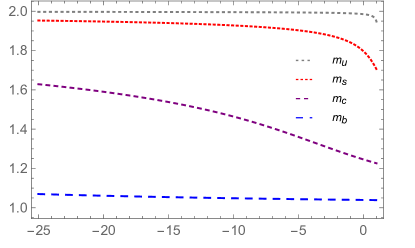
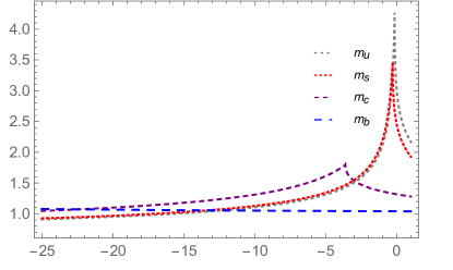
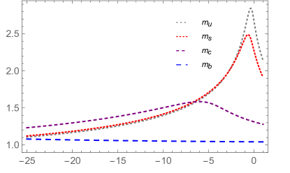
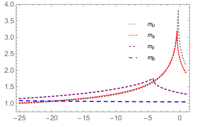
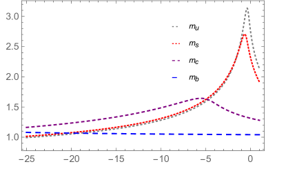
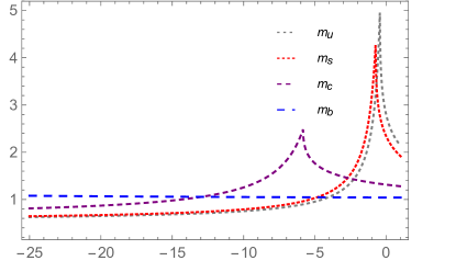
Figure 7: Comparison of $A(s)$ for the four quark masses, plotted on the same domain for each $n$. Left upper panel: $n=0$; right upper panel: $n=1$; Left middle panel: $n=2$; right middle panel: $n=3$; Left lower panel: $n=4$; right lower panel: $n=\infty$.

One observes easily how the distinctive features of the curves move further into the timelike domain with increasing quark mass. In particular, a scale relevant to the computation of meson properties via the BSE in our setup is the value $s=-m_{H}^{2}/4$ for which $M(s)$ is also tabulated in Tab. 2. While for the light mesons the meson mass range up to $2$ GeV implies values of $s\approx-1$ and higher as the region of interest, the corresponding range for bottomonium would be $s\approx-25$ and higher. Apparently, said features in $A$ and $M$ as well as the regions where the differences among the curves resulting from the various values of $n$ are most pronounced are relevant regarding the BSE for light quarks and become unimportant for heavier quarks. To elucidate this further, we provide a detailed comparison to effective free model-quark propagators in App. B.

At this point it is also interesting to note that, as already indicated in Sec. III, depending on the value of $\eta$ one potentially covers the whole range of arguments $s=-m_{H}^{2}$ (for $\eta=1$) to $s=0$ (for $\eta=0$) in the quark propagators as they appear in the BSE. In practice this means that one can attempt to choose $\eta$ such that the distinct structures in the respective dressing functions are avoided by the interplay of $s_{+}=-\eta^{2}m_{H}^{2}$ vs. $s_{-}=-(1-\eta)^{2}m_{H}^{2}$, thus, e. g., minimizing dressing effects in the resulting meson properties.

Appendix B Heavy-quark propagator

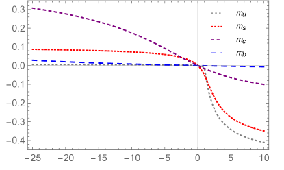
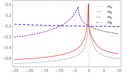
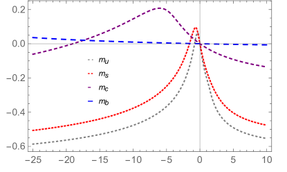
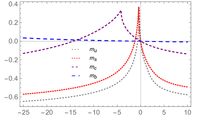
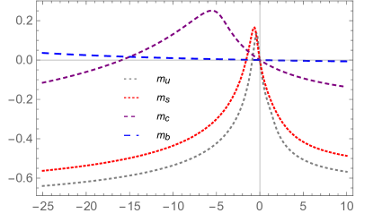
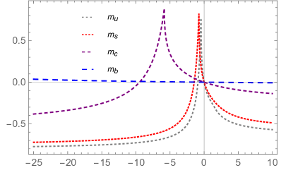
Figure 8: Comparison of the relative difference of our calculated $A(s)$ to an Ansatz $A(s)=1$ for the four quark masses, plotted on the same domain for each $n$. In particular, we plot $A(s)-1$. Left upper panel: $n=0$; right upper panel: $n=1$; Left middle panel: $n=2$; right middle panel: $n=3$; Left lower panel: $n=4$; right lower panel: $n=\infty$.

In this appendix we investigate and illustrate the properties of the quark-propagator dressing functions $A$ and $M$ for heavy quarks. This allows us to provide support for Ansätze used for the quark propagator in the heavy-quark case, where $A(s)$ is approximated by $1$ and $M(s)$ is approximated by a suitable value $M_{q}$, both of which are assumed constant.

To check this approximation we compare our calculated propagator dressing functions to the assumed effective version with $A(s)=1$ and $M(s)=M(0)$. As a first illustration we present $A(s)$ for all four quark flavors under consideration on the same domain, namely from the relevant timelike point in bottomonium to the spacelike region. In Fig. 7 we plot the four curves corresponding to the four quark masses separately for each $n$ and find qualitatively interesting features: First of all, on the considered domain, for all $n$, the behavior of $A(s)$ resembles that of a constant only for the $b$ quark; the $c$-quark propagator is still considerably dressed. Secondly, while one has to be aware of relevant domains for the lighter quarks regarding their respective bound-state-mass defined scales, the first point remains valid also if one only looks at an appropriately rescaled smaller portion of the timelike domain.

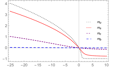
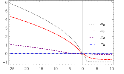
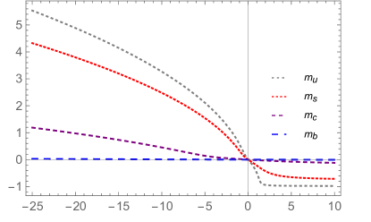
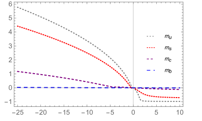
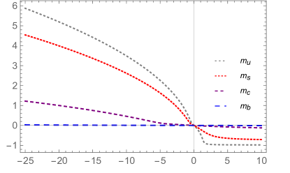
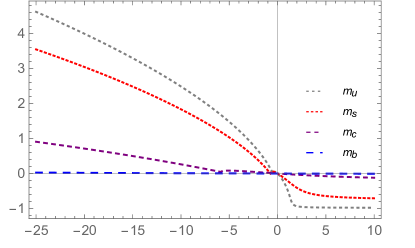
Figure 9: Comparison of the relative difference of our calculated $M(s)$ to an Ansatz $M(s)=\mbox{const.}=M(s=0)$ for the four quark masses, plotted on the same domain for each $n$. In particular, we plot $[M(s)-M(0)]/M(0)$. Left upper panel: $n=0$; right upper panel: $n=1$; Left middle panel: $n=2$; right middle panel: $n=3$; Left lower panel: $n=4$; right lower panel: $n=\infty$.

As a next step, we compare both calculated dressing functions $A$ and $M$ to their effective constant counterparts by plotting the relative difference between dressed and constant versions. The results for $A(s)$ are shown in Fig. 8, again each group of the four quark mass versions separately for the usual values of $n$. The same is shown in Fig. 9 for $M(s)$. For the constant effective value of $M_{q}$ we choose $M(s=0)$, wich is one possible definition and for our purposes is as good as any other choice on that domain of $s$ on which dynamical chiral symmetry breaking is clearly visible.

Apparently, our figures suggest that the transition from dressed to effective quark propagator happens somewhere between the $c$ and $b$ quark masses, which is not entirely unexpected: charm quarks are in general not regarded as heavy in the sense that effective theories work there without trouble; bottom quarks, on the other hand, are usually regarded as well-approximated by an effective form of the quark propagator, which we find as well. The key in Figs. 8 and 9 in order to decide whether or not one is close to the form of a free propagator is the proximity of the relative difference to zero and a constant type of behavior on the relevant domain. The only case in our computed results where this is clearly visible, is the case of the $b$ quark.

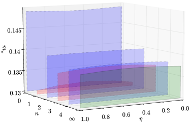
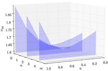
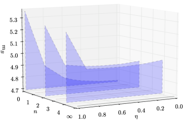
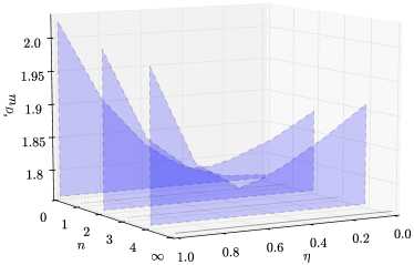
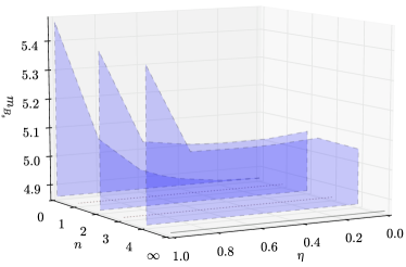
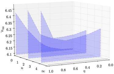
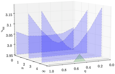
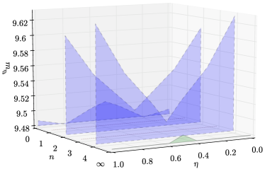
Figure 10: Meson bound-state masses as functions of $n$ and $\eta$, given in GeV. Even $n$ are depicted by dashed lines, odd ones by dotted lines, and the fully summed result by a solid line. If no solution is found, no surface is plotted at the corresponding $n$. Left upper panel: pion; right upper panel: $D$; Left upper center panel: $B$; right upper center panel: $D_{s}$; Left lower center panel: $B_{s}$; right lower center panel: $B_{c}$ Left lower panel: $\eta_{c}$; right lower panel: $\eta_{b}$.

Appendix C $\eta$-dependence of meson masses

In this appendix we collect data and plots about the details of the dependence of the meson masses on the momentum-partitioning parameter $\eta$ as a function of the order $n$ in our scheme in analogy to Tab. 4 and Fig. 4 in the main text of the paper. The data is collected in Tab. 6; the corresponding plots are shown in the various panels of Fig. 10. As a reference and excellent example for the kind of behavior to expect, we present the pion, $\eta_{c}$, and $\eta_{b}$ cases in addition to the unequal-mass collection of data and plots. For the pion the alternating pattern of convergence of the odd and even $n$ numbers described above in connection with the kaon case is reobserved. For the other cases, the situation is somewhat obscured by the lack of solutions for odd $n$ on our main $\eta$ grid points. Still, one can see convergence with $n$ as well as a pronounced $\eta$ asymmetry for the heavy-light case, which is the source of the large error bars plotted in Fig. 5. Notwithstanding this, the results clearly corroborate the systematic character of both the approach and the truncation scheme presented here as well as the validity of qualitative as well as quantitative statements made above.

Table 6: Bound-state masses for various mesons the as functions of $n$ and $\eta$, given in GeV.

$\pi$
$\eta$	0	$0.2$	$0.4$	$0.5$	$0.6$	$0.8$	1
$n=0$	0.1490	0.1488	0.1486	0.1486	0.1486	0.1488	0.1490
$n=1$	0.1309	0.1316	0.1319	0.1320	0.1319	0.1316	0.1309
$n=2$	0.1397	0.1398	0.1398	0.1398	0.1398	0.1398	0.1397
$n=3$	0.1364	0.1368	0.1370	0.1370	0.1370	0.1368	0.1364
$n=4$	0.1378	0.1381	0.1382	0.1382	0.1382	0.1381	0.1378
$n=\infty$	0.1374	0.1377	0.1379	0.1379	0.1379	0.1377	0.1374

$D$
$\eta$	$0$	$0.2$	$0.4$	$0.5$	$0.6$	$0.8$	1
$n=0$	1.645	1.651	1.673	1.691	1.716	1.797	1.946
$n=1$	…	…	…	…	…	…	…
$n=2$	1.763	1.731	1.709	1.702	1.701	1.749	1.900
$n=3$	…	…	…	…	…	….	…
$n=4$	1.795	1.752	1.718	1.705	1.696	1.731	1.881
$n=\infty$	…	…	…	…	…	…	…

$B$
$\eta$	$0$	$0.2$	$0.4$	$0.5$	$0.6$	$0.8$	1
$n=0$	4.801	4.807	4.825	4.842	4.868	4.983	5.456
$n=1$	…	…	…	…	…	…	…
$n=2$	5.017	5.004	5.003	5.006	5.012	5.034	5.370
$n=3$	…	…	…	…	…	….	…
$n=4$	5.069	5.050	5.041	5.040	5.041	5.046	5.350
$n=\infty$	…	…	…	…	…	…	…

$D_{s}$
$\eta$	0	$0.2$	$0.4$	$0.5$	$0.6$	$0.8$	1
$n=0$	1.815	1.819	1.839	1.857	1.881	1.954	2.076
$n=1$	…	…	…	…	…	…	…
$n=2$	1.933	1.896	1.870	1.862	1.861	1.911	2.047
$n=3$	…	…	…	…	…	….	…
$n=4$	1.960	1.915	1.877	1.862	1.852	1.894	2.036
$n=\infty$	…	…	…	…	…	1.880	…

$B_{s}$
$\eta$	0	$0.2$	$0.4$	$0.5$	$0.6$	$0.8$	1
$n=0$	4.960	4.965	4.984	5.002	5.029	5.150	5.567
$n=1$	…	…	…	…	…	…	…
$n=2$	5.171	5.156	5.154	5.156	5.161	5.181	5.497
$n=3$	…	…	…	…	…	….	…
$n=4$	5.150	5.199	5.189	5.187	5.187	5.189	5.483
$n=\infty$	…	…	…	…	…	…	…

$B_{c}$
$\eta$	0	$0.2$	$0.4$	$0.5$	$0.6$	$0.8$	1
$n=0$	6.147	6.150	6.172	6.193	6.226	6.329	6.471
$n=1$	…	…	…	…	…	…	…
$n=2$	6.325	6.299	6.286	6.283	6.281	6.319	6.507
$n=3$	…	…	…	…	…	….	…
$n=4$	6.361	6.327	6.306	6.298	6.290	6.312	6.521
$n=\infty$	…	…	…	…	…	…	…

$\eta_{c}$
$\eta$	0	$0.2$	$0.4$	$0.5$	$0.6$	$0.8$	1
$n=0$	3.062	3.037	3.033	3.033	3.033	3.037	3.062
$n=1$	…	…	…	…	…	…	…
$n=2$	3.161	3.082	3.024	3.012	3.024	3.082	3.161
$n=3$	…	…	…	…	…	…	…
$n=4$	3.185	3.090	3.018	2.998	3.018	3.090	3.185
$n=\infty$	…	…	…	2.985	…	…	…

$\eta_{b}$
$\eta$	0	$0.2$	$0.4$	$0.5$	$0.6$	$0.8$	1
$n=0$	9.487	9.479	9.498	9.505	9.498	9.479	9.487
$n=1$	…	…	…	…	…	…	…
$n=2$	9.607	9.555	9.521	9.504	9.521	9.555	9.607
$n=3$	…	…	…	…	…	…	…
$n=4$	9.629	9.566	9.524	9.500	9.524	9.566	9.629
$n=\infty$	…	…	…	9.489	…	…	…

Appendix D pseudoscalar kernel details

Following Refs. Bender et al. (2002); Bhagwat et al. (2004) we start from the recursion relations for the QGV $\Gamma_{\mu}$, Eq. (8) and the BSE correction term $\Lambda_{M\mu}$, Eq. (16). The first step in our construction is the decomposition of each of these quantities in terms of Dirac covariants.

The full QGV has 12 covariant structures built from $\gamma_{\mu}$ and the two independent four-vectors of the quark and antiquark lines. After the effective interaction, Eq. (5) has been employed, only three of those are nonzero and one obtains

$$\Gamma_{\mu}(p)=\alpha_{1}(p^{2})\gamma_{\mu}+\alpha_{2}(p^{2})\gamma\cdot p\;p_{\mu}-i\alpha_{3}(p^{2})p_{\mu}\;.$$ (21)

With this structure and the initial condition that the QGV be bare

$$\Gamma_{\mu}(p)^{0}=\gamma_{\mu}$$ (22)

one can express the QGV via its recursion relation to any desired order in terms of the covariants given in Eq. (21) and the quark propagator $S(p)$. The result, in turn, can be inserted in the quark DSE and yields algebraic equations for $A(s)$ and $M(s)$ via Dirac-trace projections onto the two covariant quark propagator structures.

A similar strategy is used to compute $\Lambda_{M\mu}(P)$. One starts off with finding a suitable decomposition in terms of Dirac covariants for the quantum numbers appropriate for the meson $M$ under consideration, in our case pseudoscalar. In our setup the pseudoscalar BSA has 2 nonzero components from the general four:

$$\Gamma_{PS}(P)=f_{1}(P^{2})\,i\;\gamma_{5}+f_{2}(P^{2})\,\gamma_{5}\;\gamma\cdot\hat{P}$$ (23)

with the unit vector $\hat{P}:=P/\sqrt{P^{2}}$.

The corresponding $\Lambda_{0^{-}\nu}$ has in general 12 covariant structures, four of which are nonzero in our particular setup. We have, omitting the subscript denoting the pseudoscalar case

$$\Lambda_{\mu}(P) = \beta_{1}(P^{2})\,\gamma_{5}\gamma_{\mu}+\beta_{2}(P^{2})\,\gamma_{5}\;\gamma\cdot\hat{P}\;\hat{P}_{\mu}$$ (24)

$$+ \beta_{3}(P^{2})\,\gamma_{5}\hat{P}_{\mu}+\beta_{4}(P^{2})\,\gamma_{5}\;\gamma_{\mu}\;\gamma\cdot\hat{P}\;.$$

One can obtain the scalar functions $\vec{\beta}:=\{\beta_{j}\}$, $j=1,2,3,4$, from a recursion relation extracted from the recursion relations for the QGV and $\Lambda$ via defining the projection operators

$$\mathcal{P}_{\mu,1} := \frac{1}{16}\gamma_{\mu}\;\gamma_{5}$$ (25)

$$\mathcal{P}_{\mu,2} := \frac{1}{4}\hat{P}_{\mu}\;\gamma\cdot\hat{P}\;\gamma_{5}$$ (26)

$$\mathcal{P}_{\mu,3} := \frac{1}{4}\hat{P}_{\mu}\;\gamma_{5}$$ (27)

$$\mathcal{P}_{\mu,4} := \frac{1}{16}\cdot\hat{P}\;\gamma_{\mu}\;\gamma_{5}\;.$$ (28)

Then at every $i$ one has

$$\beta_{j}^{i}=(\mathcal{M}_{\text{ps}})_{jk}\mathrm{Tr}\left[\mathcal{P}_{\mu,k}\Lambda^{i}_{\mu,\text{ps}}\right]\;,$$ (29)

where the matrix $\mathcal{M}_{\text{ps}}$ is given by

$$\mathcal{M}_{\text{ps}}=\left(\begin{array}[]{cccc}\frac{4}{3}&-\frac{1}{3}&0&0\\ -\frac{4}{3}&\frac{4}{3}&0&0\\ 0&0&\frac{4}{3}&-\frac{4}{3}\\ 0&0&-\frac{1}{3}&\frac{4}{3}\\ \end{array}\right)$$ (30)

and one can write (see also Ref. Bender et al. (2002) for more details)

$$\vec{\beta}^{i}=\mathcal{M}_{\text{ps}}\vec{\mathcal{T}}^{i}\;.$$ (31)

The vector $\vec{\mathcal{T}}^{i}$, in turn is obtained, writing $\vec{\alpha}:=\{\alpha_{j}\}$, $j=1,2,3$, from

$$\vec{\mathcal{T}}^{i}=\mathbf{G}_{-}\,\vec{\alpha}_{-}^{\,i-1}+\mathbf{G}_{+}\,\vec{\alpha}_{+}^{\,i-1}+\mathbf{L}\,\vec{\beta}^{\,i-1},$$ (32)

which can be calculated when the matrices $\mathbf{G}$ and $\mathbf{L}$ are known. $\vec{\alpha}_{+}$ and $\vec{\alpha}_{-}$ denote the coefficients of the QGV decomposition corresponding to the ₊ and _- arguments appearing in their defining quark propagators as given above. Similarly, we define

$$B_{-} := M(p_{-}^{2})A(p_{-}^{2})$$ (33)

$$B_{+} := M(p_{+}^{2})A(p_{+}^{2})$$ (34)

$$A_{-} := (\eta-1)\,\sqrt{P^{2}}A(p_{-}^{2})$$ (35)

$$A_{+} := \eta\,\sqrt{P^{2}}A(p_{+}^{2})$$ (36)

and

$$\Delta_{-} := B^{2}(p_{-}^{2})+P^{2}A^{2}(p_{-}^{2})$$ (37)

$$\Delta_{+} := B^{2}(p_{+}^{2})+P^{2}A^{2}(p_{+}^{2})$$ (38)

and obtain

$$\mathbf{L}=\frac{-\mathcal{C}}{\Delta_{-}\,\Delta_{+}}\left(\begin{array}[]{cccc}2B_{-}B_{+}-A_{-}A_{+}&\frac{1}{2}\left(B_{-}B_{+}+A_{-}A_{+}\right)&-\frac{1}{2}i\left(A_{-}B_{+}-A_{+}B_{-}\right)&-i\left(2A_{-}B_{+}+A_{+}B_{-}\right)\\ 2\left(B_{-}B_{+}+A_{-}A_{+}\right)&2\left(B_{-}B_{+}+A_{-}A_{+}\right)&-2i\left(A_{-}B_{+}-A_{+}B_{-}\right)&-2i\left(A_{-}B_{+}-A_{+}B_{-}\right)\\ 4i\left(A_{-}B_{+}-A_{+}B_{-}\right)&4i\left(A_{-}B_{+}-A_{+}B_{-}\right)&-4\left(B_{-}B_{+}+A_{-}A_{+}\right)&-4\left(B_{-}B_{+}+A_{-}A_{+}\right)\\ i\left(A_{-}B_{+}-A_{+}B_{-}\right)&i\left(A_{-}B_{+}-A_{+}B_{-}\right)&-(B_{-}B_{+}+A_{-}A_{+})&-(B_{-}B_{+}+A_{-}A_{+})\end{array}\right)\;.$$ (39)

The two matrices $\mathbf{G}_{-}$ and $\mathbf{G}_{+}$ are associated with the corresponding quark propagators with the ₊ and _- arguments as defined above:

$$\mathbf{G}_{-} = \frac{-\mathcal{C}}{\Delta_{-}^{2}\Delta_{+}}\left(\begin{array}[]{c}i\left(B_{+}A_{-}^{2}+B_{-}A_{+}A_{-}+2B_{-}^{2}B_{+}\right)f_{1}+i\left(A_{+}A_{-}^{2}-B_{-}B_{+}A_{-}+2B_{-}^{2}A_{+}\right)f_{2}\\ 2i\left(-B_{+}A_{-}^{2}+2B_{-}A_{+}A_{-}+B_{-}^{2}B_{+}\right)f_{1}+2i\left(-A_{+}A_{-}^{2}-2B_{-}B_{+}A_{-}+B_{-}^{2}A_{+}\right)f_{2}\\ -4\left(A_{+}A_{-}^{2}+2B_{-}B_{+}A_{-}-B_{-}^{2}A_{+}\right)f_{1}-4\left(-B_{+}A_{-}^{2}+2B_{-}A_{+}A_{-}+B_{-}^{2}B_{+}\right)f_{2}\\ \left(-A_{+}A_{-}^{2}-2B_{-}B_{+}A_{-}+B_{-}^{2}A_{+}\right)f_{1}+\left(B_{+}A_{-}^{2}-2B_{-}A_{+}A_{-}-B_{-}^{2}B_{+}\right)f_{2}\end{array}\right.$$ (54)

$$\begin{array}[]{c}-\frac{1}{2}iP^{2}\left(B_{+}A_{-}^{2}-2B_{-}A_{+}A_{-}-B_{-}^{2}B_{+}\right)f_{1}(\eta-1)^{2}-\frac{1}{2}iP^{2}\left(A_{+}A_{-}^{2}+2B_{-}B_{+}A_{-}-B_{-}^{2}A_{+}\right)f_{2}(\eta-1)^{2}\\ -2iP^{2}\left(B_{+}A_{-}^{2}-2B_{-}A_{+}A_{-}-B_{-}^{2}B_{+}\right)f_{1}(\eta-1)^{2}-2iP^{2}\left(A_{+}A_{-}^{2}+2B_{-}B_{+}A_{-}-B_{-}^{2}A_{+}\right)f_{2}(\eta-1)^{2}\\ -4P^{2}\left(A_{+}A_{-}^{2}+2B_{-}B_{+}A_{-}-B_{-}^{2}A_{+}\right)f_{1}(\eta-1)^{2}-4P^{2}\left(-B_{+}A_{-}^{2}+2B_{-}A_{+}A_{-}+B_{-}^{2}B_{+}\right)f_{2}(\eta-1)^{2}\\ -P^{2}\left(A_{+}A_{-}^{2}+2B_{-}B_{+}A_{-}-B_{-}^{2}A_{+}\right)f_{1}(\eta-1)^{2}-P^{2}\left(-B_{+}A_{-}^{2}+2B_{-}A_{+}A_{-}+B_{-}^{2}B_{+}\right)f_{2}(\eta-1)^{2}\end{array}$$

$$\left.\begin{array}[]{c}-\frac{1}{2}i\sqrt{P^{2}}(\eta-1)\left(A_{+}A_{-}^{2}+2B_{-}B_{+}A_{-}-B_{-}^{2}A_{+}\right)f_{1}-\frac{1}{2}i\sqrt{P^{2}}(\eta-1)\left(-B_{+}A_{-}^{2}+2B_{-}A_{+}A_{-}+B_{-}^{2}B_{+}\right)f_{2}\\ -2i\sqrt{P^{2}}(\eta-1)\left(A_{+}A_{-}^{2}+2B_{-}B_{+}A_{-}-B_{-}^{2}A_{+}\right)f_{1}-2i\sqrt{P^{2}}(\eta-1)\left(-B_{+}A_{-}^{2}+2B_{-}A_{+}A_{-}+B_{-}^{2}B_{+}\right)f_{2}\\ 4\sqrt{P^{2}}(\eta-1)\left(B_{+}A_{-}^{2}-2B_{-}A_{+}A_{-}-B_{-}^{2}B_{+}\right)f_{1}+4\sqrt{P^{2}}(\eta-1)\left(A_{+}A_{-}^{2}+2B_{-}B_{+}A_{-}-B_{-}^{2}A_{+}\right)f_{2}\\ \sqrt{P^{2}}(\eta-1)\left(B_{+}A_{-}^{2}-2B_{-}A_{+}A_{-}-B_{-}^{2}B_{+}\right)f_{1}+\sqrt{P^{2}}(\eta-1)\left(A_{+}A_{-}^{2}+2B_{-}B_{+}A_{-}-B_{-}^{2}A_{+}\right)f_{2}\end{array}\right)$$

which is to be understood as a $4\times 3$ matrix, and its corresponding analog.

References

- Hilger and Kämpfer (2009) T. Hilger and B. Kämpfer, 0904.3491 [nucl-th] .
- Hilger et al. (2010) T. Hilger, R. Schulze, and B. Kämpfer, J.Phys. G37, 094054 (2010).
- Hilger et al. (2012a) T. Hilger, R. Thomas, B. Kämpfer, and S. Leupold, Phys.Lett. B709, 200 (2012a).
- Hilger et al. (2011) T. Hilger, B. Kämpfer, and S. Leupold, Phys. Rev. C 84, 045202 (2011).
- Hilger et al. (2012b) T. Hilger, T. Buchheim, B. Kämpfer, and S. Leupold, Prog.Part.Nucl.Phys. 67, 188 (2012b).
- Buchheim et al. (2014) T. Buchheim, T. Hilger, and B. Kämpfer, 1411.7863 [nucl-th] .
- Roberts et al. (2007) C. D. Roberts, M. S. Bhagwat, A. Holl, and S. V. Wright, Eur. Phys. J. Special Topics 140, 53 (2007).
- Fischer (2006) C. S. Fischer, J. Phys. G 32, R253 (2006).
- Alkofer and von Smekal (2001) R. Alkofer and L. von Smekal, Phys. Rept. 353, 281 (2001).
- Sanchis-Alepuz and Williams (2015a) H. Sanchis-Alepuz and R. Williams, 1503.05896 [hep-ph] .
- Dudek et al. (2008) J. J. Dudek, R. G. Edwards, N. Mathur, and D. G. Richards, Phys. Rev. D 77, 034501 (2008).
- Liu et al. (2012) L. Liu, G. Moir, M. Peardon, S. M. Ryan, C. E. Thomas, P. Vilaseca, J. J. Dudek, R. G. Edwards, B. Joo, and D. G. Richards (Hadron Spectrum Collaboration), J. High Energy Phys. 07, 126 (2012).
- Thomas (2013) C. Thomas, Proc. Sci. LATTICE2013, 003 (2013).
- Flynn et al. (2015) J. Flynn, T. Izubuchi, T. Kawanai, C. Lehner, A. Soni, et al., 1501.05373 [hep-lat] .
- Bhagwat et al. (2004) M. S. Bhagwat, A. Holl, A. Krassnigg, C. D. Roberts, and P. C. Tandy, Phys. Rev. C 70, 035205 (2004).
- Gomez-Rocha et al. (2014) M. Gomez-Rocha, T. Hilger, and A. Krassnigg, 10.1007/s00601-014-0938-8, 1408.1077 [hep-ph] .
- Godfrey and Isgur (1985) S. Godfrey and N. Isgur, Phys. Rev. D 32, 189 (1985).
- Maris and Tandy (1999) P. Maris and P. C. Tandy, Phys. Rev. C 60, 055214 (1999).
- Holl et al. (2004) A. Holl, A. Krassnigg, and C. D. Roberts, Phys. Rev. C 70, 042203(R) (2004).
- Holl et al. (2005a) A. Holl, A. Krassnigg, P. Maris, C. D. Roberts, and S. V. Wright, Phys. Rev. C 71, 065204 (2005a).
- Krassnigg (2009) A. Krassnigg, Phys. Rev. D 80, 114010 (2009).
- Krassnigg and Blank (2011) A. Krassnigg and M. Blank, Phys. Rev. D 83, 096006 (2011).
- Dorkin et al. (2011) S. M. Dorkin, T. Hilger, L. P. Kaptari, and B. Kämpfer, Few Body Syst. 49, 247 (2011).
- Mader et al. (2011) V. Mader, G. Eichmann, M. Blank, and A. Krassnigg, Phys. Rev. D 84, 034012 (2011).
- Hilger (2012) T. U. Hilger, Medium Modifications of Mesons, Ph.D. thesis, TU Dresden (2012).
- Popovici et al. (2014) C. Popovici, T. Hilger, M. Gomez-Rocha, and A. Krassnigg, 10.1007/s00601-014-0934-z, 1407.7970 [hep-ph] .
- Hilger et al. (2015a) T. Hilger, C. Popovici, M. Gomez-Rocha, and A. Krassnigg, Phys. Rev. D 91, 034013 (2015a).
- Fischer et al. (2014) C. S. Fischer, S. Kubrak, and R. Williams, Eur. Phys. J. A 50, 126 (2014).
- Fischer et al. (2015) C. S. Fischer, S. Kubrak, and R. Williams, Eur.Phys.J. A51, 10 (2015).
- Hilger et al. (2015b) T. Hilger, M. Gomez-Rocha, and A. Krassnigg, Phys. Rev. D 91, 114004 (2015b).
- Bhagwat et al. (2007a) M. S. Bhagwat, A. Hoell, A. Krassnigg, C. D. Roberts, and S. V. Wright, Few-Body Syst. 40, 209 (2007a).
- Krassnigg (2008) A. Krassnigg, Proc. Sci. Confinement8, 075 (2008).
- Blank and Krassnigg (2011a) M. Blank and A. Krassnigg, Comput. Phys. Commun. 182, 1391 (2011a).
- Blank and Krassnigg (2011b) M. Blank and A. Krassnigg, AIP Conf. Proc. 1343, 349 (2011b).
- Blank (2011) M. Blank, Properties of quarks and mesons in the Dyson-Schwinger/Bethe-Salpeter approach, Ph.D. thesis, University of Graz (2011), 1106.4843 [hep-ph] .
- Watson and Cassing (2004) P. Watson and W. Cassing, Few-Body Syst. 35, 99 (2004).
- Watson et al. (2004) P. Watson, W. Cassing, and P. C. Tandy, Few-Body Syst. 35, 129 (2004).
- Fischer et al. (2005) C. S. Fischer, P. Watson, and W. Cassing, Phys. Rev. D 72, 094025 (2005).
- Fischer and Williams (2008) C. S. Fischer and R. Williams, Phys. Rev. D 78, 074006 (2008).
- Fischer and Williams (2009) C. S. Fischer and R. Williams, Phys. Rev. Lett. 103, 122001 (2009).
- Williams (2010) R. Williams, EPJ Web Conf. 3, 03005 (2010).
- Williams (2015) R. Williams, Eur.Phys.J. A51, 57 (2015).
- Sanchis-Alepuz et al. (2014) H. Sanchis-Alepuz, C. S. Fischer, and S. Kubrak, Phys. Lett. B 733, 151 (2014).
- Chang and Roberts (2009) L. Chang and C. D. Roberts, Phys. Rev. Lett. 103, 081601 (2009).
- Heupel et al. (2014) W. Heupel, T. Goecke, and C. S. Fischer, Eur. Phys. J. A 50, 85 (2014).
- Sanchis-Alepuz and Williams (2015b) H. Sanchis-Alepuz and R. Williams, 1504.07776 [hep-ph] .
- Munczek and Nemirovsky (1983) H. J. Munczek and A. M. Nemirovsky, Phys. Rev. D 28, 181 (1983).
- Bender et al. (1996) A. Bender, C. D. Roberts, and L. Von Smekal, Phys. Lett. B 380, 7 (1996).
- Bender et al. (2002) A. Bender, W. Detmold, C. D. Roberts, and A. W. Thomas, Phys. Rev. C 65, 065203 (2002).
- Krassnigg and Roberts (2004) A. Krassnigg and C. D. Roberts, Nucl. Phys. A 737, 7 (2004).
- Holl et al. (2005b) A. Holl, A. Krassnigg, and C. D. Roberts, Nucl. Phys. Proc. Suppl. 141, 47 (2005b).
- Matevosyan et al. (2007a) H. H. Matevosyan, A. W. Thomas, and P. C. Tandy, Phys. Rev. C 75, 045201 (2007a).
- Matevosyan et al. (2007b) H. H. Matevosyan, A. W. Thomas, and P. C. Tandy, J. Phys. G 34, 2153 (2007b).
- Jinno et al. (2015) R. Jinno, T. Kitahara, and G. Mishima, Phys. Rev. D 91, 076011 (2015).
- Nguyen et al. (2009) T. Nguyen, N. A. Souchlas, and P. C. Tandy, AIP Conf. Proc. 1116, 327 (2009).
- Souchlas and Stratakis (2010) N. Souchlas and D. Stratakis, Phys. Rev. D 81, 114019 (2010).
- Nguyen et al. (2011) T. Nguyen, N. A. Souchlas, and P. C. Tandy, AIP Conf.Proc. 1361, 142 (2011).
- Ivanov et al. (1998a) M. A. Ivanov, Y. L. Kalinovsky, P. Maris, and C. D. Roberts, Phys. Rev. C 57, 1991 (1998a).
- Ivanov et al. (1998b) M. A. Ivanov, Y. L. Kalinovsky, P. Maris, and C. D. Roberts, Phys. Lett. B 416, 29 (1998b).
- Ivanov et al. (1999) M. A. Ivanov, Y. L. Kalinovsky, and C. D. Roberts, Phys. Rev. D 60, 034018 (1999).
- Blaschke et al. (2000) D. B. Blaschke, G. R. G. Burau, M. A. Ivanov, Y. L. Kalinovsky, and P. C. Tandy, hep-ph/0002047 .
- Bhagwat et al. (2007b) M. S. Bhagwat, A. Krassnigg, P. Maris, and C. D. Roberts, Eur. Phys. J. A31, 630 (2007b).
- Ivanov et al. (2007) M. A. Ivanov, J. G. Korner, S. G. Kovalenko, and C. D. Roberts, Phys. Rev. D 76, 034018 (2007).
- El-Bennich et al. (2010) B. El-Bennich, M. A. Ivanov, and C. D. Roberts, Nucl.Phys.Proc.Suppl. 199, 184 (2010).
- El-Bennich et al. (2011) B. El-Bennich, M. A. Ivanov, and C. D. Roberts, Phys. Rev. C 83, 025205 (2011).
- Neubert (1994) M. Neubert, Phys.Rept. 245, 259 (1994).
- Gomez-Rocha and Schweiger (2012) M. Gomez-Rocha and W. Schweiger, Phys.Rev. D86, 053010 (2012).
- Munczek (1995) H. J. Munczek, Phys. Rev. D 52, 4736 (1995).
- Maris and Roberts (1997) P. Maris and C. D. Roberts, Phys. Rev. C 56, 3369 (1997).
- Blank and Krassnigg (2011c) M. Blank and A. Krassnigg, Phys. Rev. D 84, 096014 (2011c).
- Dorkin et al. (2014) S. M. Dorkin, L. P. Kaptari, T. Hilger, and B. Kämpfer, Phys. Rev. C 89, 034005 (2014).
- Dorkin et al. (2015) S. Dorkin, L. Kaptari, and B. Kämpfer, Phys. Rev. C 91, 055201 (2015).