Holographic Calculation for Large Interval Rényi Entropy at High Temperature

Abstract

In this paper, we study the holographic Rényi entropy of a large interval on a circle at high temperature for the two-dimensional CFT dual to pure AdS₃ gravity. In the field theory, the Rényi entropy is encoded in the CFT partition function on $n$-sheeted torus connected with each other by a large branch cut. As proposed in [7], the effective way to read the entropy in the large interval limit is to insert a complete set of state bases of the twist sector at the branch cut. Then the calculation transforms into an expansion of four-point functions in the twist sector with respect to $e^{-\frac{2\pi TR}{n}}$. By using the operator product expansion of the twist operators at the branch points, we read the first few terms of the Rényi entropy, including the leading and next-to-leading contributions in the large central charge limit. Moreover, we show that the leading contribution is actually captured by the twist vacuum module. In this case by the Ward identity the four-point functions can be derived from the correlation function of four twist operators, which is related to double interval entanglement entropy. Holographically, we apply the recipe in [20] and [26] to compute the classical Rényi entropy and its 1-loop quantum correction, after imposing a new set of monodromy conditions. The holographic classical result matches exactly with the leading contribution in the field theory up to $e^{-4\pi TR}$ and $l^{6}$, while the holographical 1-loop contribution is in exact agreement with next-to-leading results in field theory up to $e^{-\frac{6\pi TR}{n}}$ and $l^{4}$ as well.

¹Department of Physics and State Key Laboratory of Nuclear Physics and Technology, Peking University, Beijing 100871, P.R.​ China
²Collaborative Innovation Center of Quantum Matter,
Beijing 100871, P. R. China
³Center for High Energy Physics, Peking University,
Beijing 100871, P. R. China

1 Introduction

The entanglement entropy is an important notion in a quantum many-body system [1, 2]. Not only could it be used to measure the effective degrees of freedom in the system, but it could also be taken as a quantum order parameter, among its various applications. It is defined as follows. Let $A$ be a subsystem, and then the reduced density matrix of $A$ is obtained by tracing out the degrees of freedom of its complement$A^{c}$

$$\rho_{A}={\textrm{Tr}}_{A^{c}}\rho,$$ (1.1)

where $\rho$ is the density matrix of the whole system. Then the entanglement entropy is defined to be the von Neumann entropy of the reduced density matrix

$$S_{A}=-{\textrm{Tr}}\rho_{A}\log\rho_{A}.$$ (1.2)

Furthermore for pure state $\rho=\mid\psi\rangle\langle\psi\mid$, the entanglement entropy of the subsystem is equal to the one of its complementary part

$$S_{A}=S_{A^{c}},$$ (1.3)

but for a thermal state the equality breaks down,

$$S_{A}\neq S_{A^{c}}$$ (1.4)

because of the thermal effect. It is convenient to calculate the entanglement entropy from the Rényi entropy, which is defined to be

$$S_{n}=-\frac{1}{n-1}\log{\textrm{Tr}}\rho_{A}^{n}.$$ (1.5)

The entanglement entropy can be read from

$$S_{EE}=\lim_{n\rightarrow 1}S_{n},$$ (1.6)

if the limit $n\rightarrow 1$ is well defined.

In quantum field theory, the entanglement entropy and Rényi entropy are hard to compute because there are an infinite number of degrees of freedom. In this case, the entanglement entropy is defined with respect to a spatial submanifold at a fixed time. By using the replica trick[3] the Rényi entropy can be transformed into the partition function of $n$ copies of field theory with the fields being identified at the submanifold. It is usually a formidable task to compute this partition function for a general field theory. Even for two-dimensional (2D) conformal field theory (CFT), which is expected to give more analytic results due to the existence of infinite dimensional symmetries, the exact results are limited. For 2D CFT, the Rényi entropy is generally related to the partition function on a higher genus Riemann surface. Besides a few universal results determined by the conformal symmetries[4], only the partition functions of a free boson and fermion on a higher genus Riemann surface have been known [5] [6] [7] [8][9] [10].

However, it is possible to expand the partition function with respect to some modular parameters for a general CFT in some cases. The two simplest nontrivial examples are the case of two intervals on a complex plane and the case of one interval on a torus. Generally, to calculate the partition function, one can cut the Riemann surface at some cycles and insert a complete set of state bases such that the full Riemann surface changes into a surface without handle and hole and the computation transforms into a summation of multipoint correlation functions on a full complex plane. The key point is to find the nice way to cut open the Riemann surface such that the expansion series is well behaved. For a general genus-$g$ Riemann surface, we can always choose $g$ couples of $A$ cycles and $B$ cycles with a proper intersection [11] and cut the Riemann surface at certain cycles. Different choices on the cutting correspond to different ways of expanding the partition function. Even though by the modular invariance the different expansions should be equal to each other, their convergent rates are different.

The simplest trivial example is the partition function on a torus. One may quantize the theory along the thermal direction or the spatial direction, which corresponds to inserting the complete bases along the spatial cycle or thermal cycle, and the partition function could be written as

$$Z=\sum_{i}e^{-\frac{2\pi\beta}{R}(L_{i}+\bar{L}_{i}-\frac{c}{12})},\hskip 12.91663pt\mbox{or}\hskip 8.61108ptZ=\sum_{i}e^{-\frac{2\pi R}{\beta}(L_{i}+\bar{L}_{i}-\frac{c}{12})}.$$ (1.7)

Because of the modular invariance, the two different calculations give the same answer. At a low temperature the quantization along the thermal direction leads to a better convergent series while at a high temperature the spatial quantization works better.

For the double-interval case, if the intervals are short, one may take the operator product expansion(OPE) of the twist operators to compute the Rényi and entanglement entropy order by order with respect to a small cross ratio[13, 12]. Actually, taking OPE is equivalent to inserting a complete set of bases at the cycles around the two intervals on every sheet. In the Riemann surface for the $n$th Rényi entropy of the double-interval case, there are $n-1$ independent couples of cycles denoted by $A_{i}$ and $B_{i}$. As shown in Fig. 1 for the $n=3$ case, there are two couples of independent cycles $A_{i},B_{i},i=1,2$. In the small interval limit, we can take the OPE of the twist operators at the branch points of the first interval. This is equivalent to cutting and inserting a complete set of state bases at $A_{i}$ cycles enclosing the interval. This expansion is well convergent for a small cross ratio. On the contrary, for a large cross ratio which means the intervals are large and the branch points of two intervals are close to each other, we must take the OPE of the second and third twist operators, which is equivalent to cutting the Riemann surface along the $B_{i}$ cycles enclosing the branch points of separated intervals.

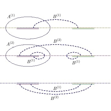
Figure 1: Canonical cycles for the double intervals

For the case of a single interval on a torus, the Riemann surface is obtained by connecting $n$ tori along the branch cut. When the interval is not very large, one may cut the spatial or thermal cycle and insert a complete set of bases to compute the partition function[6] [14], just as in the genus-1 case. Which cycles to cut depends on the temperature. But for a high temperature and a very large interval, the previous treatment is not good enough because the resulting expansion series is poorly behaved. Instead, it was proposed in [15] [7] that one should cut the cycle crossing the branch cut. This requires the insertion of a complete set of bases in the twist sector rather than the normal sector in the $n$-copied CFT. This proposal has been checked for the free compact and noncompact bosons, and it has been applied to prove the universal relation between the thermal entropy and the entanglement entropy.

The AdS/CFT correspondence provides another way to compute the entanglement entropy in a CFT. For the Einstein gravity, it was first proposed by Ryu and Takayanagi[16, 17] that the entanglement entropy could be holographically given by the area of a minimal surface in the bulk, which is homogeneous to $A$

$$S_{EE}=\frac{\mbox{Area}(\Sigma_{A})}{4G}.$$ (1.8)

The holographic entanglement entropy could be understood as a generalized gravitational entropy [18] [19]. In the higher dimension case, it is not clear if the holographic entanglement entropy gives precisely the entanglement entropy in the dual field theory. Nevertheless, for a 2D CFT holographically dual to AdS₃ gravity, it has been proved that the holographic computation is correct in the semiclassical regime[21, 20]. Therefore, the Rényi entropy provides a new window to study the AdS₃/CFT₂ correspondence.

The $AdS_{3}/CFT_{2}$ correspondence states that the quantum gravity in $AdS_{3}$ spacetime is dual to a 2D CFT with a central charge [22]

$$c=\frac{3l}{2G},$$ (1.9)

and a sparse light spectrum [21] [23], where $G$ is the three-dimensional (3D) gravity coupling constant. Though a precise definition of AdS₃ quantum gravity, possibly a string theory, has not been well established, its semiclassical limit has been much studied. As the classical configurations in the AdS₃ gravity could be obtained as the quotients of the global AdS₃ by the subgroup of the isometry group $SL(2,C)$, the path integral of semiclassical AdS₃ gravity could be defined in principle. On the other side, the explicit construction of dual CFT is not known. Nevertheless, the large central charge limit of the CFT, corresponding to the semiclassical gravity, is much simplified. Under this limit, only the vacuum module dominates the contribution to the CFT partition function[21]. As a result, the partition function is universal in the sense that it is very much restricted by the conformal symmetry, and is independent of the explicit construction of the CFT. In this work, we are interested in the large central charge limit of the Rényi entropy of 2D CFT. From the AdS₃/CFT₂ correspondence, the partition function of the Riemann surface in the CFT should be given by the partition function of the gravitational configuration ending on the Riemann surface. In the large central charge limit, the Rényi entropy can be decomposed into the terms proportional to $c$, $c^{0}$, $\frac{1}{c}$, …, which should correspond respectively to the classical, quantum 1-loop, 2-loop, etc. , parts of the gravitational partition function[13].

In the field theory side, for a genus-$g$ Riemann surface, we need to choose $g$ $A_{i}$ cycles to insert complete bases at each cycle such that the expansion converges fast. Under the large $c$ limit, the dominant contribution to the partition function comes from the light primary states [21] and their descendants. The heavy states give only nonperturbative corrections of order $O(e^{-c})$. Furthermore, among the light spectrums only the vacuum module gives the linear $c$ order result and the other modules give only higher order corrections with respect to $\frac{1}{c}$[21]. Moreover, it turns out that even for the next-to-leading correction with respect to $\frac{1}{c}$, the first few terms in the expansion are captured only by the vacuum module [24] [25] [14]. The vacuum Verma module consists of a primary identity operator and its descendants which could be constructed by the stress tensors $T(z)$ and $\bar{T}(\bar{z})$. In this work, we assume that for the field theory that is dual to the pure gravity, we only need to insert the vacuum module at each cycle.

Because of the replica symmetry, we always deal with a CFT on an $n$-sheeted surface, which can be regarded as one CFT with $n$ copies of the original field with the fields in different replicas being identified along the branch cut. When we combine the $n$-sheeted surface’s field into one CFT, we call it $n$-copied CFT with $nc$ central charge and denote it as CFT_n. The original CFT is denoted as CFT₁. If we do not consider the monodromy condition of the fields around the branch point, the $n$ copies of the fields are decoupled so that we have just a tensor product of $n$ copies of the fields. In this case, we call it the normal sector of CFT_n. In contrast, if we consider the twist monodromy condition of the fields around the branch point, we get the twist sector of CFT_n. In both cases, we can classify the states by the irreducible representations of its Virasoro algebra Vir^(t), defined by the stress tensor $T(z)=\displaystyle{\sum_{j=1}^{n}T^{(j)}(z)}$. Under Vir^(t), the twist (normal) sector states can be decomposed into more than one irreducible module, and the one with the lowest conformal dimension is called the twist (trivial) vacuum module. Note that the twist (trivial) vacuum module has a different meaning from the vacuum module in the original CFT. For the partition function of a CFT on an $n$-sheeted Riemann surface resulting from the replica trick, we have two pictures to compute it. One is to regard it as the one of CFT₁ on the $n$-sheeted surface, and the other one is to regard it as the correlator of twist operators in CFT_n.

On the bulk side, to calculate the partition function on a higher genus Riemann surface holographically, one needs to find the gravity configuration whose asymptotic boundary is exactly the Riemann surface. To find the gravity configuration, one can use the Schottky uniformization to get the Riemann surface and then extend the uniformization to the bulk. However for one Riemann surface, there may be more than one Schottky uniformization and different uniformizations give different gravity configurations. Among all of the gravity configurations the one with the least classical action dominates the partition function in the large $c$ limit[20]. The contributions from other configurations are suppressed as $O(e^{-c})$. Furthermore the 1-loop correction can be determined by the functional determinant of the fluctuations around the classical background [26] by using the heat kernel method developed in [28, 27]. Recently, by using the operator product expansion of the twist operators, the holographic computation of the double-interval Rényi entanglement entropy for the CFT has been checked beyond the classical level[25, 29, 31, 30, 32]. Furthermore, for the single interval on a circle at finite temperature, if the interval is not very large, the holographic computation has been confirmed to be in exact agreement with the field theory computation[14], in which the thermal density matrix is expanded level by level [33].

In this paper, we study the Rényi entropy of a large interval on a circle at high temperature in the context of AdS₃/CFT₂ correspondence, extending our previous study in [14]. In the large interval limit, the computations in both the field theory and the bulk need to be developed furthermore. On the field theory side, the study in [14] showed that the perturbative series in the partition function do not converge well. Actually, the classical part of the Rényi entropy is just

$$S_{n}\mid_{classical} = \frac{c}{6}\frac{1+n}{n}\log\sinh(2\pi TY)+\mbox{const.}-\left.\frac{c}{9}\frac{(n+1)(n^{2}-1)}{n^{3}}\right\{\sinh^{4}(2\pi Ty)e^{-4\pi TR}$$ (1.10)

$$+4\sinh^{4}(2\pi Ty)\cosh^{2}(2\pi Ty)e^{-6\pi TR}+\left(\frac{-11-2n^{2}+1309n^{4}}{11520n^{4}}\cosh(16\pi Ty)\right.$$

$$-\frac{-11+28n^{2}+199n^{4}}{1440n^{4}}\cosh(12\pi Ty)-\frac{77-346n^{2}+197n^{4}}{2880n^{4}}\cosh(8\pi Ty)$$

$$\left.\left.-\frac{-77+436n^{2}+433n^{4}}{1440n^{4}}\cosh(4\pi Ty)+\frac{-77+466n^{2}+907n^{4}}{2304n^{4}}\right)e^{-8\pi TR}\right\}$$

$$+O(e^{-10\pi TR}),$$

where $y$ is the length of the interval. When the length of the interval is comparable with the size of the circle $y\sim R$, the expansion converges very slowly and is not good anymore. This asks us to find another perturbative way to compute the partition function more effectively and reliably. In [7], we proposed to insert a complete twist sector states through the branch cut and expand the Rényi entropy with respect to $e^{-\frac{2\pi L}{n\beta}}$. In [15, 7], we tested this proposal and reconsidered the noncompact and compact free scalars and found good agreements with direct expansions of the partition functions. Now we are going to consider the CFT with a holographic gravity dual, in the large interval and high temperature limit. We only consider the vacuum module of CFT₁ and its correspondents in the twist sector of CFT_n. After cutting through the branch cut, the Riemann surface still have a nonzero genus and the four-point functions in the twist sector cannot be calculated directly. Furthermore, we use the OPE of the two twist operators at the branch points and compute the correlation functions on the unfolded cylinder of length $n\beta$ with the fields in the OPE at the different positions. We manage to expand the result with respect to complementary part of the interval length $l$. We calculate the Rényi entropy up to order $l^{4}$ and $e^{-\frac{8\pi L}{nR}}$, including the leading linear $c$, the $c$-independent, and $1/c$ parts. Moreover, we find that the leading contribution is actually captured by the twist vacuum module. We support this result not only by the argument using the large central charge limit of the conformal blocks but also by direct computation using the Ward identity. As a result, we obtain the exact formula for the entanglement entropy.

For the holographic calculation, we follow the treatments in [26] [20], but basing on a different monodromy condition. As shown in [34], the holographic entanglement entropy for the large interval case is not read from the bulk geodesic ending on the interval. Instead, it is the sum of the horizon length and the geodesic of the complementary interval. This fact suggests that there is a phase transition when the interval becomes large, and the bulk gravitational configuration for the large interval must be different. Instead of the cycles used in [14], we choose another $n$ cycles to be of trivial monodromy. Among them, there is one cycle crossing the branch cut $n$ times, and the other $n-1$ independent ones crossing the branch cut and enclosing the complementary part of the branch cut in different sheets. As shown in Fig. 2 for $n=3$, we set $\tilde{A}_{i}$’s to be of trivial monodromy. As a warm-up, we compute the classical holographic entanglement entropy by using the new monodromy conditions, and we obtain the result suggested in [34]. Furthermore, we compute the holographic Rényi entropy up to $l^{6}$ and $e^{-4\pi TR}$ for classical contribution, and up to $l^{4}$ and $e^{-\frac{6\pi TR}{n}}$ for 1-loop quantum contribution. The results are in perfect match with CFT’s computation.

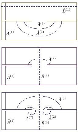
Figure 2: Canonical cycles for the large interval at high temperature: $n=3$ case

The remaining parts of the paper are organized as follows. In Sec. 2, we present the field theory computation. After a brief review on the twist sector of the CFT_n, we focus on the vacuum module and compute the Rényi entropy in the first few orders. In Sec. 3, we show how to do holographic computation with the new monodromy condition. We obtain both the classical and 1-loop quantum results perturbatively. Up to the orders we are interested in, we find good agreements with the field theory results. In Sec. 4, we end with conclusions and discussions. We collect some technical details in Appendices.

2 Field theory calculation

In this section, we present our computation on the large interval Rényi entropy on a circle at high temperature in the CFT which corresponds to pure $AdS_{3}$ gravity. By the replica trick the Rényi entropy can be transformed into calculating the partition function on a higher genus Riemann surface, which is obtained by pasting $n$ tori along a large branch cut. In Fig. 2, we cut open the torus and show the branch cut (interval). The horizontal line is the spatial direction of length $R$, and the vertical line is the thermal direction of a length $\beta$. The large interval is presented as double solid lines between ${\cal{T}}^{(+)}$ and ${\cal{T}}^{(-)}$. In Fig. 3b, we translate the interval, and in Fig. 3c, we unfold the branch cut and get a cylinder of thermal length $n\beta$, with $n$ cuts. We denote the coordinate in Fig. 3b as $u$ and the one in Fig. 3c as $y$, and set the two branch points to be at $\pm\frac{l}{2}$ in Fig. 3b.

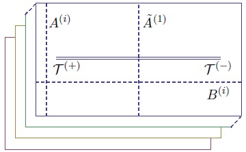
(a) $n$ sheeted Riemann surface

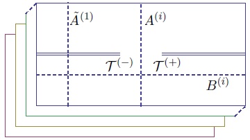
(b) translate the interval

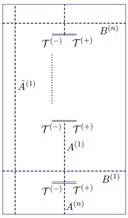
(c) unfold the twist

Figure 3: Riemann surface for finite temperature Rényi entropy. The horizontal line denotes the spatial direction of unit length, and the vertical line denotes the thermal direction of length $\beta$. (a) The Riemann surface for $n$ cylinders connected by a branch cut, which is denoted by a solid line ${\cal{T}}^{(+)}{\cal{T}}^{-}$. In each sheet, there is a cycle $A^{(i)}$ along the imaginary time direction. However there could also be a cycle marked by $\tilde{A}^{(1)}$, which crosses the branch cut and goes from one sheet to the next one $n$ times until it goes back to the original sheet. (b) The same as (a), just by shifting the branch cut to the boundary. ${\cal{T}}^{-}{\cal{T}}^{+}$ denotes the complement of the original interval. In (c) we unfold the twist. There are $n$ copies of ${\cal{T}}^{-}{\cal{T}}^{+}$ cuts in the unfolded picture.

As in our previous paper [7] [15], we would cut the Riemann surface through the branch cut, $\tilde{A}^{(1)}$ cycle in Fig. 3b, and insert complete bases in the twist sector of CFT_n at the cycle. The calculation transforms into a series of four-point functions with two twist operators and two operators in the twist sector. As the two branch points are actually very close to each other, we may take the OPE for the two twist operators, which amounts to an infinite summation of local operators in the $n$-copied CFT.

Alternatively, we may unfold the Riemann surface as in Fig. 3c and insert complete state bases of the normal sector in single sheet CFT to do the computation. Changing into the coordinate in Fig. 3c, we find that the localized operators in the $j$th copy in the OPE sit in the imaginary axis

$$y^{(j)}=i(j\beta).$$ (2.1)

In this way, each term in the expansion is a multipoint correlation function on an infinite cylinder, with two normal sector operators at the left and the right infinities of the cylinder and $n$ localized operators at $y^{(j)}$.

We calculate the leading terms for the Rényi entropy expanded with respect to both $e^{-\frac{2\pi R}{n\beta}}$ and $l$. The results in the large $c$ limit actually include the leading contribution, which is linear $c$, and the next-to-leading contribution, which is of order one, and even the next-to-next-to-leading contribution. We argue that only the descendants of the twist vacuum, the states generated by acting the Virasoro algebra Vir^(t) of CFT_n on the twist vacuum, contribute to the leading $c$ result. We confirm this fact by the analysis of the classical conformal block expansion in the large $c$ limit. We furthermore derive the first few leading linear $c$ terms from the descendants by using the Ward identity on the correlation functions of four twist operators, which could be related to the one in the double-interval case. In the $n\to 1$ limit, we find that only the twist vacuum module has a nonvanishing contribution. This leads to the entanglement entropy of the large interval, which is exactly the same as the one from the holographic computation. However, when we consider the next-to-leading contribution to the Rényi entropy, we have to take the contributions from other states in the twist sector into account.

2.1 Twist sector

In this subsection, let us give a brief review on the twist sector in the CFT_n. By the replica trick the Rényi entropy can be transformed into the partition function of a single copy CFT on an $n$-sheeted surface connected at the branch cut. From the path integral, it is easy to see that the partition function could be taken as the $n$ copies of field theory, one on each sheet, with fields on different sheets being related at the branch cut. In this $n$-copied theory, the locality requires us to introduce the twist field or antitwist field at the branch points[35, 4].

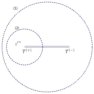
Figure 4: Branch cut

Let us show how the twist sector arises in a CFT_n with a branch cut, following the discussion in [36]. As the twist field is a local field, we consider simply the $n$-sheeted surface connected by a single branch cut. As in Fig.4, the ${\cal{T}^{\pm}}$ denote the branch point located at $z_{1},z_{2}$ and the double line denotes the branch cut. Now we study it as a CFT_n. Considering an operator $T^{(j_{1})}(z)$ , it will change to $T^{(j_{1}+1)}(z)$ when it moves once around the branch point ${\cal{T}^{+}}$ along the circle (2). The point $z=z_{1}$ is a branch singularity in the $n$-copied theory, which is a source of stress tensor [4]

$$<T(z)>=n<T^{(1)}(z)>\sim\frac{c}{24}(n-\frac{1}{n})\frac{1}{(z-z_{1})^{2}},$$ (2.2)

when $z$ is close to $z_{1}$. Independence on the branch cut implies a local operator at the branch point. This local operator is known as the twist operator, denoted as ${\cal{\hat{T}}^{+}}(z_{1})$. It is a primary field, with conformal dimension $h=\frac{c}{24}(n-\frac{1}{n})$. In a similar way, we can get the antitwist operators at the other branch point. Much information of the CFT_n is encoded in the twist operators. For example, the partition function of an $n$-sheeted complex plane with $N$ intervals is determined by the $2N$-point function of the twist and antitwist operators on a complex plane. Moreover, considering the operator-state correspondence, the twist operator corresponds to the ground state in the twisted sector of Hilbert space. Considering the OPE of the twist field with other basic fields in the theory, we will find other excited twist fields. Correspondingly, we find the excited states in the twist sector, as we will review soon.

Before our discussion of the twist sector and antitwist sector states in the $n$-copied field theory, we show that the OPE of a twist sector operator and an antitwist sector operator give trivial sector operators in the $n$-copied field theory. As argued above, the excited states in the twist sector could be obtained by considering the monodromy of the field moving around the branch point $z_{1}$ along the circle (2) in Fig.4 . However, when we consider the OPE of the operators in both the twist sector and antitwist sector, by the monodromy condition, the resulting states in the circle (1) in Fig.4 must be in the trivial sector. This fact has been applied in the discussion of the OPE of two twist operators in the short interval limit. In that case, the operators in the expansion are in the tensor product of the normal sector of the CFT in each sheet (which is just the trivial sector in the CFT_n picture), as shown in [12, 25]. More generally, for the excited states in the twist sector, their OPE should consist of the trivial sector states.

Now, let us give a review on the twist sector states [14] in the CFT_n arising from the replica trick in calculating the Rényi entropy. Let us work in the coordinate $u$ in Fig. 3b. To expand the partition function, we need to insert complete twist sector bases along the cycle $\tilde{A}^{(1)}$. We may temporarily forget about the geometric structure of the torus and only consider the geometry and the monodromy condition near the cycles $\tilde{A}^{(1)}$ . Moreover, as the vacuum module dominates in the large central charge limit, we focus on the twist sector from the vacuum module. For more complete discussion on other modules, please see [14] for more details. In the vacuum module, the fields are constructed from the stress tensor. The monodromy condition on the stress tensor is

$$T^{(j)}(u+i\beta)=T^{(j+1)}(u),\hskip 12.91663ptj=0,\cdots,n-1$$ (2.3)

in the $u$ coordinate, with $T^{(n)}(u)=T^{(0)}(u)$, and

$$T(y+in\beta)=T(y),$$ (2.4)

in the $y$ coordinate. In the $y$ coordinate, the $n$ copies of fields are unfolded as

$$T^{(j)}(u)=T(y)\mid_{y=u+ij\beta}.$$ (2.5)

Taking the conformal transformations

$$z=e^{\frac{2\pi u}{\beta}},$$ (2.6)

$$w=e^{\frac{2\pi y}{n\beta}},$$ (2.7)

the monodromies in the new coordinates $z,w$ are, respectively,

$$T^{(j)}(ze^{2\pi i})=T^{(j+1)}(z),$$ (2.8)

$$T(we^{2\pi i})=T(w).$$ (2.9)

The states inserted at the $\tilde{A}^{(1)}$ cycle in Figs. 3b and Fig. 3c can be described as the vertex operators being inserted at the origin of $z$ and $w$. As in [7], we can redefine the operators in the $z$ coordinate,

$$T^{(t,k)}(z)\equiv\sum_{j=1}^{n}T^{(j)}(z)e^{\frac{2\pi i}{n}kj},\hskip 12.91663ptk=0,1,\cdots,n-1$$ (2.10)

and expand it as

$$T^{(t,k)}(z)=\sum_{m\in{\cal Z}}\frac{L^{(k)}_{m}}{z^{m+2+\frac{k}{n}}}.$$ (2.11)

The operators $L^{(k)}_{m}$ satisfy a commutation relation similar to the Virasoro algebra. Among the operators $T^{(t,k)}(z)$, $T^{(t,0)}$ is of special importance. It is the total stress tensor for the whole $n$-copied theory, and $\{L^{(0)}_{m}\}$ are the generators of the corresponding Virasoro algebra Vir^(t).

We may study the spectrum of the theory with respect to Vir^(t). From the commutators between $L^{(k)}_{m}$ and $L_{0}^{(0)}$,

$$[L^{(0)}_{0},L^{(k)}_{m}]=-(m+\frac{k}{n})L^{k}_{m}.$$ (2.12)

we know that when the operators $L_{m}^{(k)}$ act on a state, those with

$$~{}m>0,~{}0\leq k<n,~{}~{}\mbox{or}~{}~{}~{}m=0,~{}0<k<n,$$ (2.13)

decrease conformal dimension, so they are annihilation operators; while those with

$$~{}m<0,~{}0\leq k<n,$$ (2.14)

increase the conformal dimension, so they are creation operators. Therefore we can define the vacuum for the twist sector to be

$$L^{(k)}_{m}\mid t\rangle=0~{}~{}~{}\mbox{for} m>0,~{}0\leq k<n,~{}~{}\mbox{or}~{}~{}~{}m=0,~{}0<k<n.$$ (2.15)

The twist vacuum has the lowest conformal dimension

$$h_{v}=\frac{c}{24}n(1-\frac{1}{n^{2}}).$$ (2.16)

Acting with the creation operators on the twist vacuum we can get all of the excited states in the twist sector.

There is a one-to-one correspondence between the twist sector states in the CFT_n and the normal sector states in the original one-sheet CFT. Actually the trivial monodromy condition in the $w$ coordinate suggests that the mode expansion in the $w$ coordinate for the field gives the normal sector of the CFT. The conformal dimensions between the twist sector states and the normal sector states are related by

$$h_{twist}=\frac{1}{n}h_{normal}+\frac{c}{24}n(1-\frac{1}{n^{2}}).$$ (2.17)

On the cylinder, the energy of the state could be written as

$$H = \frac{2\pi}{\beta}(L_{twist}+\bar{L}_{twist}-\frac{nc}{12})=\frac{2\pi}{n\beta}(L_{normal}+\bar{L}_{normal}-\frac{c}{12}).$$ (2.18)

The $\frac{1}{n}$ factor in the last equation is due to the fact that in the $y$ coordinate the length of the thermal cycle is $n\beta$. For convenience, we will denote the states in the twist sector as $\mid t,i\rangle$, corresponding to the state $\mid i\rangle$ in the original theory.

It turns out to be more useful to classify the states in the twist sector by using the conformal symmetry in the $n$-copied theory. The states should be decomposed into different irreducible modules of the Virasoro algebra Vir^(t). To show this decomposition we calculate the chiral partition function for the twist sector

$${\textrm{Tr}}q^{L_{0}}=q^{h_{v}}\prod_{s=2}^{\infty}\frac{1}{1-q^{\frac{s}{n}}}=\big{(}q^{h_{v}}\cdot\prod_{s\geq 2,\frac{s}{n}\notin\mathbb{N}}\frac{1}{1-q^{\frac{s}{n}}}\big{)}\cdot\prod_{r=1}^{\infty}\frac{1}{1-q^{r}}.$$ (2.19)

In the second equation, we have used the fact that there is a one-to-one correspondence between the twist sector states in the CFT_n and the normal sector states in the one-sheet CFT, with their the conformal dimensions being related by (2.17). For the vacuum module in the normal sector, the descendants are generated by the Virasoro algebra $L_{-s}$ with $s\geq 2$, so the product begins from $s=2$. For a primary operator with the conformal dimension $h$, if there is no null state in its descendants, its contribution to the chiral partition function is

$${\textrm{Tr}}q^{L_{0}}\mid_{h}=q^{h}\prod_{s=1}^{\infty}\frac{1}{1-q^{s}}.$$ (2.20)

Considering this fact, the quantity in the parentheses of (2.19) can be taken as a generating function for the primary operators with respect to the Virasoro algebra. As explained in [7], the operators $L^{(0)}_{-m}$ in the $z$ coordinate correspond to the generators $L_{-mn}$ in the unfolded $w$ coordinate with $mn>1$. As $L_{-mn}$ do not generate null states in the normal sector vacuum module, the operators $L^{(0)}_{-m}$ do not generate null states in the twist sector either. Therefore there is no null state in the descendants of each primary states in the twist sector. Expanding the function

$$\big{(}q^{h_{v}}\cdot\prod_{s\geq 2,\frac{s}{n}\notin\mathbb{N}}\frac{1}{1-q^{\frac{s}{n}}}\big{)},$$ (2.21)

with respect to $q$, the coefficient before $q^{h}$ is the number of the primary operator with conformal dimension $h$. It is clear that in the twist sector there are many new primary states and the number of the primary states increases exponentially with the conformal dimension. For example, acting with the operators $L^{(n-i)}_{-1}$ on the twist vacuum, the resulting states that have conformal dimensions $h=h_{v}+\frac{i}{n}$ are the primary states, since they can be annihilated by the operators $L_{m}^{(0)},m>0$ in Vir^(t). Among the modules in the twist sector, the vacuum module generated by $L_{m}^{(0)},m<0$ on the twist vacuum is the most important one in our following discussion. We call this module the twist vacuum module.

In the following discussion, we will meet another notion, the normal sector, in the $n$-copied field theory. It is defined with respect to the $n$-copied field theory without a branch cut, or the tensor product of the $n$ copies of Hilbert space of the normal sector of a single CFT. Moreover, as we only focus on the vacuum module of the CFT, we call the tensor product of $n$-copied vacuum module as the trivial sector in the $n$-copied field theory. Note that the stress tensor $T^{(t,0)}$ is still a well-defined quantity in the $n$-copied field theory without the branch cut. Therefore we may classify the states in the trivial sector by the Virasoro algebra Vir^(t). In this case, we find that there are exponentially increasing primary operators with respect to Vir^(t) in the trivial sector of the CFT_n as well. Considering the chiral partition function, we have

$${\textrm{Tr}}q^{L_{0}} = (\prod_{s=2}^{\infty}\frac{1}{1-q^{s}})^{n}$$ (2.22)

$$= \prod_{s=2}^{\infty}\frac{1}{1-q^{s}}+(1-q)\left(\prod_{r=2}^{\infty}\frac{1}{(1-q^{r})^{n-1}}-1\right)\prod_{s=1}^{\infty}\frac{1}{1-q^{s}}.$$

In the last equation, we decompose the whole partition function into the contribution from different modules with respect to Vir^(t). Each module is generated by $L_{-m}^{(0)},m>0$ acting on the highest weight state. The first term denotes the module generated from the vacuum state, with zero conformal dimension, so the product starts from $s=2$. For the other primary operators, there are no null states in their descendants. This is because the primary state has nonzero conformal dimension, and the states $L_{-1}^{m}\mid h\rangle$ have nonzero norm. Considering $[L_{r},L_{-r}]=\frac{c}{12}r(r^{2}-1)+2rL_{0}$, for $r>1$, the commutator has a linear $c$ term. In the large c limit, all of the states have nonzero norm. To read the number of other primary states, we just need to expand the quantity

$$(1-q)\left(\prod_{r=2}^{\infty}\frac{1}{(1-q^{r})^{n-1}}-1\right),$$ (2.23)

with respect to $q$, such that the coefficient before $q^{h}$ is just the number of the primary states with a conformal dimension $h$. We can easily see that the number of the primary states increases exponentially with their conformal weights. In the following, we call the module generated from the vacuum a trivial vacuum module, with respect to Vir^(t).

2.2 Rényi entropy

As discussed previously, we can expand the partition function by inserting complete twist sector bases in Fig. 3b or complete normal sector bases in Fig. 3c. The partition function can be expanded as

$$Z_{n} = \sum_{i}e^{-\frac{2\pi R}{\beta}(h_{t,i}+\bar{h}_{t,i}-n\frac{c}{12})}\langle t,i\mid{\cal{\hat{T}}}^{-}(u_{1}){\cal{\hat{T}}}^{+}(u_{2})\mid t,i\rangle\mid_{u}$$ (2.24)

$$= \sum_{i}e^{-\frac{2\pi R}{n\beta}(h_{i}+\bar{h}_{i}-\frac{c}{12})}\langle t,i\mid{\cal{\hat{T}}}^{-}(u_{1}){\cal{\hat{T}}}^{+}(u_{2})\mid t,i\rangle\mid_{u},$$

in the $u$ coordinate, and in the second line we use (2.17). And the thermal partition function reads

$$Z_{1}=\sum_{i}e^{-\frac{2\pi R}{\beta}(h_{i}+\bar{h}_{i}-\frac{c}{12})}.$$ (2.25)

In the large $c$ limit, we only need to consider the vacuum module, which captures the perturbative effect. We list the first few states in the vacuum module and their vertex operators at the origin and the infinity in Appendix A. Such states give the first few leading order contributions to the Rényi entropy.

Each term in (2.24) is a four-point function with two twist operators at the branch points and two operators in the twist sector at the left and the right infinities. For the CFT dual to pure gravity, we do not know exactly the analytic form of this correlation function. Nevertheless, when the twist operators are very close, we may take the OPE of two twist operators

$${\cal{\hat{T}}}^{-}(-\frac{l}{2}){\cal{\hat{T}}}^{+}(\frac{l}{2})\sim c_{n}l^{-\frac{c}{6}n(1-\frac{1}{n^{2}})}V(0)\bar{V}(0),$$ (2.26)

where

$$V(u) = 1+\sum_{i}\frac{1}{12}(1-\frac{1}{n^{2}})l^{2}T^{(i)}(u)+\sum_{i}\frac{1}{488}(1-\frac{1}{n^{2}})l^{4}\partial^{2}T^{(i)}(u)$$ (2.27)

$$+\sum_{i}\frac{1}{288}(1-\frac{1}{n^{2}})^{2}l^{4}(:T^{(i)}(u)^{2}:-\frac{3}{10}\partial^{2}T^{(i)}(u))$$

$$+\sum_{i_{1}<i_{2}}[\frac{1}{8c}\frac{1}{n^{4}}\frac{1}{\sin^{4}\frac{\pi}{n}(i_{1}-i_{2})}+\frac{1}{144}(1-\frac{1}{n^{2}})^{2}]l^{4}T^{(i_{1})}(u)T^{(i_{2})}(u)+O(l^{5}),$$

and the similar form for the antiholomorphic part $\bar{V}(u)$. In the operator product expansion, we only consider the vacuum module in each sheet and ignore the other modules.

In practice, it is more convenient to unfold the twist and consider the correlation function in Fig. 3c. After transforming into the coordinate $y$, we find that the operators in $V(0)$ are localized at

$$T^{(j)}(0)\rightarrow T(y)|_{y=ij\beta},$$ (2.28)

namely, the operators in different sheets are unfolded and located at different positions in the cylinder. We may use the OPE of the twist operators to compute the partition function perturbatively. Now the partition function can be expanded as a multipoint correlation function on the cylinder involving $n$ operators located at $y=ij\beta$, and two vertex operators at left and right infinities. We can furthermore take a conformal transformation into the $w$ coordinate, and do the calculation in a full complex plane. Formally, we still write

$$Z_{n} = e^{\frac{\pi Rc}{6n\beta}}\langle t\mid{\cal{\hat{T}}}^{-}(u_{1}){\cal{\hat{T}}}^{+}(u_{2})\mid t\rangle(\sum_{i,\bar{i}}\frac{\langle t,i,\bar{i}\mid{\cal{\hat{T}}}^{-}(u_{1}){\cal{\hat{T}}}^{+}(u_{2})\mid t,i,\bar{i}\rangle}{\langle t\mid{\cal{\hat{T}}}^{-}(u_{1}){\cal{\hat{T}}}^{+}(u_{2})\mid t\rangle}e^{-\frac{2\pi R}{n\beta}(h_{i}+\bar{h}_{i})})$$ (2.29)

$$= e^{\frac{\pi Rc}{6n\beta}}c_{n}l^{-\frac{c}{6}n(1-\frac{1}{n^{2}})}\langle t\mid V(0)\mid t\rangle\langle t\mid\bar{V}(0)\mid t\rangle(\sum_{i}\frac{\langle t,i\mid V(0)\mid t,i\rangle}{\langle t\mid V(0)\mid t\rangle}e^{-\frac{2\pi R}{n\beta}h_{i}})(\sum_{\bar{i}}\frac{\langle t,\bar{i}\mid V(0)\mid t,\bar{i}\rangle}{\langle t\mid V(0)\mid t\rangle}e^{-\frac{2\pi R}{n\beta}\bar{h}_{i}})$$

$$= e^{\frac{\pi Rc}{6n\beta}}c_{n}l^{-\frac{c}{6}n(1-\frac{1}{n^{2}})}(\langle t\mid V(0)\mid t\rangle(\sum_{i}\frac{\langle t,i\mid V(0)\mid t,i\rangle}{\langle t\mid V(0)\mid t\rangle})e^{-\frac{2\pi R}{n\beta}h_{i}})^{2}.$$

In the second line we take into (2.26), and the fact that the holomorphic and antiholomorphic parts decompose. In this case, the holomorphic and antiholomorphic parts are equal to each other. The Rényi entropy is

$$S_{n} = -\frac{1}{n-1}\log\frac{Z_{n}}{Z_{1}^{n}}$$ (2.30)

$$= -\frac{1}{n-1}((\log c_{n}-\frac{c}{6}n(1-\frac{1}{n^{2}})\log l+\frac{\pi Rc}{6n\beta}+2\log\langle t\mid V(0)\mid t\rangle$$

$$+2\log(\sum_{i}\frac{\langle t,i\mid V(0)\mid t,i\rangle}{\langle t\mid V(0)\mid t\rangle}e^{-\frac{2\pi R}{n\beta}h_{i}}))-n(\frac{\pi Rc}{6\beta}+2\log(\sum_{i}e^{-\frac{2\pi R}{\beta}h_{i}}))).$$

Denote

$$f_{i}=\frac{\langle t,i\mid V(0)\mid t,i\rangle}{\langle t,0\mid V(0)\mid t,0\rangle}\left|{}_{u}=\frac{\langle i\mid V(0)\mid i\rangle}{\langle 0\mid V(0)\mid 0\rangle}\right|_{y},$$ (2.31)

where in the last equation, we change into the $y$ coordinate. Taking $f_{i}$ into (2.30), we get the first few terms of the $n$th Rényi entropy

$$S_{n} = -\frac{1}{n-1}\log c_{n}+\frac{c}{6}\frac{n+1}{n}\log l+\frac{\pi Lc}{6\beta}\frac{n+1}{n}-\frac{2}{n-1}\log\langle t\mid V(0)\mid t\rangle$$ (2.32)

$$-\frac{2}{n-1}(f_{2}e^{-\frac{4\pi R}{n\beta}}+f_{3}e^{-\frac{6\pi R}{n\beta}}+(f_{4,1}+f_{4,2}-\frac{1}{2}f_{2}^{2})e^{-\frac{8\pi R}{n\beta}}+O(e^{-\frac{10\pi R}{n\beta}}))$$

$$+\frac{2n}{n-1}(e^{-\frac{4\pi R}{\beta}}+e^{-\frac{6\pi R}{\beta}}+\frac{3}{2}e^{-\frac{8\pi R}{\beta}}+O(e^{-\frac{10\pi R}{\beta}})).$$

The Rényi entropy is expanded with respect to $e^{-\frac{2\pi R}{\beta}}$ and $e^{-\frac{2\pi R}{n\beta}}$ . The two expansion arguments are not independent. In the above formula, we have actually done the computation in Fig. 3c. In other words, we have unfolded the twist and consider the insertion of the normal sector states at the left and the right infinities of the cylinder. Meanwhile to calculate the analytic form of $f_{i}$, we also take the OPE of the twist operators which is an expansion with respect to the relative length of the two twist operators Therefore, we have two kinds of expansion, one from the normal sector states and the other from the OPE of the twist operators. This results in two different expansions in $S_{n}$.

The explicit expressions of $f_{j}$’s can be found in Appendix C. There are a few remarkable properties on $f_{j}$’s.

1. First of all, the $l^{2}$ terms in $f_{j}$’s always take the form $\frac{j}{3}\frac{(-1+n^{2})\pi^{2}}{\beta^{2}n^{3}}$. This is because the operator at $l^{2}$ order in the OPE is the stress tensor $T(z)=\sum_{j=1}^{n}T^{(j)}(z)$, whose correlation function is fixed by the Ward identity.

2. Second, for each $f_{j}$ there exist some exceptional integers $n$ at which $f_{j}$ does not share a general formula and take specific form. This fact forbids an analytic continuation of the Rényi entropy to noninteger $n$ in order to calculate the entanglement entropy. It is because in the OPE (2.26) there is always a term like

   $$\sum_{j_{1}<j_{2}}T^{(j_{1})}T^{(j_{2})}.$$ (2.33)

   The correlation function involving such a term includes the summation

   $$\sum_{j_{1}-j_{2}=1}^{n-1}\sin^{m}(\frac{\pi(j_{1}-j_{2})}{n}).$$ (2.34)

   When $m<0$, the summation has a universal formula for any integer $n$, while for $m>0$, it is more complicated. We can rewrite the sine function in the summations as

   $$\sin^{m}(\frac{\pi(j_{1}-j_{2})}{n})=\sum_{r}a_{r}e^{\frac{2\pi ir(j_{1}-j_{2})}{n}}.$$ (2.35)

   If we take a summation for each term we find

   $$\sum_{j_{1}-j_{2}=1}^{n-1}e^{\frac{2\pi ir(j_{1}-j_{2})}{n}}=\left\{\begin{array}[]{ccc}-1,{}&~{}\mbox{for}{}&\frac{r}{n}\notin\mathbb{N}\\ n-1,{}&~{}\mbox{for}{}&\frac{r}{n}\in\mathbb{N}\end{array}\right.,$$ (2.36)

   which shows the nonanalytic origin.

3. We notice that $f_{j}$ has no linear $c$ contribution for nearly all of $n$ but finite exceptions. Actually, when $\mid t,j\rangle$ is primary, there is no linear $c$ term in $f_{j}$. To understand this effect, we can first transform into a $z$ coordinate and expand the four point function by conformal blocks. Using the large $c$ conformal block [21], there should be no linear $c$ contribution. For nearly all of $n$ but finite exceptions, $\mid t,j\rangle$ is primary. For example, when $n$ is bigger than the conformal dimension of $\mid j\rangle$, which is the corresponding state in the normal sector, the state $\mid t,j\rangle$ is primary because it can be annihilated by all of the Virasoro algebra generators $L_{m}^{(0)}$ with $m>0$.

4. Furthermore, we also notice that for the $n$ in which $f_{j}$ has no linear $c$ terms, $f_{j}$ always share a general formula up to $l^{4}$. As we discussed before, the non-analytic property comes from correlation functions

   $$\langle t,j\mid T^{(j_{1})}(u)T^{(j_{2})}(u)\mid t,j\rangle.$$ (2.37)

   Because of the symmetry, the correlation function is a sum of

   $$\sin^{m}\frac{\pi}{n}(j_{1}-j_{2}).$$ (2.38)

   If there are some terms with $m>0$ the final result is non-analytic for $n$. However, if $\mid t,j\rangle$ is primary, this cannot happen. Consider

   $$\sum_{j_{1}<j_{2}}\langle t,j\mid T^{(j_{1})}(u)T^{(j_{2})}(u)\mid t,j\rangle$$ (2.39)

   $$= \frac{n}{2}\sum_{j_{1}-j_{2}=1}^{n-1}\langle t,j\mid T^{(j_{1})}(u)T^{(j_{2})}(u)\mid t,j\rangle,$$

   $$= \frac{n}{2}\sum_{j_{1}-j_{2}=1}^{n-1}\sum_{m}b_{m}\sin^{m}\frac{\pi}{n}(j_{1}-j_{2}).$$

   On the other hand, we have

   $$\sum_{j_{1}<j_{2}}T^{(j_{1})}(u)T^{(j_{2})}(u) = \frac{1}{2}(\sum_{j=0}^{n-1}T^{(j)}(u))^{2}-\frac{1}{2}\sum_{j=0}^{n-1}(T^{(j)}(u))^{2}$$ (2.40)

   $$= \frac{1}{2}T(u)^{2}-\frac{1}{2}\sum_{j=0}^{n}(T^{(j)}(u))^{2}.$$

   For the primary state, the correlation function $\langle t,j\mid T(u)^{2}\mid t,j\rangle$ can be fixed by the Ward identity, and it is analytic for all $n$. The term $\langle t,j\mid(T^{(j)}(u))^{2}\mid t,j\rangle$ does not depend on $j$, and it is also analytic, which means there is no $m>0$ terms in (2.39). It is not clear whether this property can be extended to a higher order of OPE expansion with respect to $l$.

Here we just list the first few leading order results of the Rényi entropy:

$$S_{2} = -\log c_{2}+c\left(\frac{1}{4}\log l+\frac{\pi R}{4\beta}+(\frac{\pi^{2}l^{2}}{96\beta^{2}}-\frac{61\pi^{4}l^{4}}{184320\beta^{4}})-\frac{\pi^{4}l^{4}}{64\beta^{4}}e^{-\frac{2\pi R}{\beta}}-\frac{11\pi^{4}l^{4}}{64\beta^{4}}e^{-\frac{4\pi R}{\beta}}\right)$$ (2.41)

$$+\left\{-\frac{\pi^{4}l^{4}}{2048\beta^{4}}-(2+\frac{\pi^{2}l^{2}}{2\beta^{2}}+\frac{25\pi^{4}l^{4}}{384\beta^{4}})e^{-\frac{2\pi R}{\beta}}-(2+\frac{3\pi^{2}l^{2}}{4\beta^{2}}+\frac{15\pi^{4}l^{4}}{256\beta^{4}})e^{-\frac{3\pi R}{\beta}}\right.$$

$$\left.+(1-\frac{3\pi^{2}l^{2}}{2\beta^{2}}-\frac{275\pi^{4}l^{4}}{384\beta^{4}})e^{-\frac{4\pi R}{\beta}}\right\}+\frac{1}{c}\left(-\frac{3\pi^{4}l^{4}}{64\beta^{4}}e^{-\frac{2\pi R}{\beta}}+\frac{\pi^{4}l^{4}}{128\beta^{4}}e^{-\frac{3\pi R}{\beta}}-\frac{21\pi^{4}l^{4}}{64\beta^{4}}e^{-\frac{4\pi R}{\beta}}\right)$$

$$+O(l^{5})+O(e^{-\frac{5\pi R}{\beta}})$$

$$S_{3} = -\frac{1}{2}c_{3}+c\left(\frac{2}{9}\log l+\frac{2\pi R}{9\beta}+(\frac{\pi^{2}l^{2}}{243\beta^{2}}-\frac{347\pi^{4}l^{4}}{1771470\beta^{4}})-\frac{128\pi^{4}l^{4}}{6561\beta^{4}}e^{-\frac{2\pi R}{\beta}}\right)$$ (2.42)

$$+\left\{-\frac{16\pi^{4}l^{4}}{177147\beta^{4}}-(1+\frac{16\pi^{2}l^{2}}{81\beta^{2}}+\frac{800\pi^{4}l^{4}}{59049\beta^{4}})e^{-\frac{4\pi R}{3\beta}}-(1+\frac{8\pi^{2}l^{2}}{27\beta^{2}}+\frac{280\pi^{4}l^{4}}{6561\beta^{4}})e^{-\frac{2\pi R}{\beta}}\right.$$

$$\left.-(\frac{3}{2}+\frac{16\pi^{2}l^{2}}{27\beta^{2}}+\frac{608\pi^{4}l^{4}}{6561\beta^{4}})e^{-\frac{8\pi R}{3\beta}}\right\}+\frac{1}{c}\left(-\frac{256\pi^{4}l^{4}}{59049\beta^{4}}e^{-\frac{4\pi R}{3\beta}}-\frac{32\pi^{4}l^{4}}{6561\beta^{4}}e^{-\frac{2\pi R}{\beta}}-\frac{64\pi^{4}l^{4}}{6561\beta^{4}}e^{-\frac{8\pi R}{3\beta}}\right)$$

$$+O(l^{4})+O(e^{-\frac{10\pi R}{3\beta}})$$

$$S_{4} = -\frac{1}{3}c_{4}+c\left(\frac{5}{24}\log l+\frac{5\pi R}{24\beta}+(\frac{5\pi^{2}l^{2}}{2304\beta^{2}}-\frac{2089\pi^{4}l^{4}}{14155776\beta^{4}})-\frac{126\pi^{4}l^{4}}{6144\beta^{4}}e^{-\frac{2\pi R}{\beta}}\right)$$ (2.43)

$$+\left\{-\frac{11\pi^{4}l^{4}}{262144\beta^{4}}-(\frac{2}{3}+\frac{5\pi^{2}l^{2}}{48\pi^{2}}+\frac{749\pi^{4}l^{4}}{147456\beta^{4}})e^{-\frac{\pi R}{\beta}}-(\frac{2}{3}+\frac{5\pi^{2}l^{2}}{32\beta^{2}}+\frac{1375\pi^{4}l^{4}}{98304\beta^{4}})e^{-\frac{3\pi R}{2\beta}}\right.$$

$$\left.-(1+\frac{5\pi^{2}l^{2}}{16\beta^{2}}+\frac{719\pi^{4}l^{4}}{16384\beta^{4}})e^{-\frac{2\pi R}{\beta}}\right\}+\frac{1}{c}\left(-\frac{19\pi^{4}l^{4}}{24576\beta^{4}}e^{-\frac{\pi R}{\beta}}-\frac{95\pi^{4}l^{4}}{49152\beta^{4}}e^{-\frac{3\pi R}{2\beta}}-\frac{23\pi^{4}l^{4}}{8192\beta^{4}}e^{-\frac{2\pi R}{\beta}}\right)$$

$$+O(l^{4})+O(e^{-\frac{5\pi R}{2\beta}})$$

$$S_{n} = -\frac{1}{n-1}\log c_{n}+c\left(\frac{1}{6}\frac{n+1}{n}\log l+\frac{\pi R}{6\beta}\frac{n+1}{n}+\frac{\pi^{2}l^{2}(n+1)}{36\beta^{2}n^{3}}-\frac{l^{4}\pi^{4}(n+1)(n^{6}+9n^{4}-9n^{2}+11)}{12960\beta^{4}n^{7}}\right)$$ (2.44)

$$+-\frac{l^{4}\pi^{4}(n+1)(n^{2}+11)(3n^{4}+10n^{2}+227)}{226800\beta^{4}n^{7}}-\frac{2}{n-1}\left\{\left(1+\frac{2\pi^{2}l^{2}(n^{2}-1)}{3\beta^{2}n^{3}}\right.\right.$$

$$\left.-\frac{\pi^{4}l^{4}(n^{6}-12n^{5}-3n^{4}+24n^{3}+135n^{2}-444n+299)}{54\beta^{4}n^{7}}\right)e^{-\frac{4\pi R}{n\beta}}$$

$$+\left(1+\frac{\pi^{2}l^{2}(n^{2}-1)}{\beta^{2}n^{3}}-\frac{\pi^{4}l^{4}(n^{6}-18n^{5}-5n^{4}+36n^{3}+835n^{2}-4626n+6081)}{36\beta^{4}n^{7}}\right)e^{-\frac{6\pi R}{n\beta}}$$

$$\left.+\left(\frac{3}{2}+\frac{2\pi^{2}l^{2}(n^{2}-1)}{\beta^{2}n^{3}}-\frac{l^{4}\pi^{4}(5n^{6}-120n^{5}-31n^{4}+240n^{3}+9635n^{2}-72840n+135111)}{90\beta^{4}n^{7}}\right)e^{-\frac{8\pi R}{n\beta}}\right\}$$

$$+\frac{1}{c}\frac{2}{n-1}\left(\frac{\pi^{4}l^{4}(2n^{6}-63n^{4}-672n^{2}+733)}{945\beta^{4}cn^{7}}e^{-\frac{4\pi R}{n\beta}}+\frac{\pi^{4}(2n^{6}-217n^{4}+1148n^{2}-933)}{630\beta^{4}cn^{7}}e^{-\frac{6\pi R}{n\beta}}\right.$$

$$\left.+\frac{l^{4}\pi^{4}(2n^{6}-427n^{4}+13328n^{2}-40320n+27417)}{315\beta^{4}n^{7}}e^{-\frac{8\pi R}{n\beta}}\right)+O(l^{4})+O(e^{-\frac{10\pi R}{n\beta}})$$

for $n>4$.

2.3 Classical limit of the conformal blocks

In the previous subsection, we claimed that for each $f_{j}$, when $\mid t,j\rangle$ is a primary state in $n$-copied theory, it has no linear $c$ contribution. In this subsection, we clarify this fact from the point of view of a large $c$ conformal block, and furthermore we show that we only need to consider the twist vacuum module to find the linear $c$ order entanglement and Rényi entropies.

Let us study the four point function between two twist operators and two vertex operators corresponding to $\mid t,j\rangle$ in the twist sector, which is primary under the conformal symmetry of the $n$-copied theory. By the conformal transformation

$$v=e^{\frac{2\pi}{\beta}(u-\frac{l}{2})},$$ (2.45)

the four-point correlation function can be transformed into

$$\langle t,j\mid{\cal{T}}^{-}(-\frac{l}{2}){\cal{T}}^{+}(\frac{l}{2})\mid t,j\rangle\mid_{u}$$

$$= (\frac{2\pi}{\beta}e^{-\frac{2\pi l}{\beta}})^{\frac{c}{6}(n-\frac{1}{n})}\langle t,j\mid{\cal{T}}^{-}(e^{-\frac{2\pi l}{\beta}}){\cal{T}}^{+}(1)\mid t,j\rangle\mid_{v},$$

which can be expanded by the conformal blocks as

$$\sum_{p}C_{h_{\cal{T}},h_{\cal{T}}}^{h_{p}}C_{h_{t,j},h_{t,j}}^{h_{p}}{\cal{F}}(nc,h_{\cal{T}},h_{\cal{T}},h_{t,j},h_{t,j};h_{p};1-e^{-\frac{2\pi l}{\beta}}),$$ (2.46)

where $nc$ is the central charge of the CFT_n, and $C_{h_{1},h_{2}}^{h_{3}}$ is the OPE coefficient from two primary operators with $h_{1}$ $h_{2}$ conformal dimension to a primary operator with $h_{3}$ conformal dimension. The first four conformal dimensions in $\cal F$ are for the four external operators, two twist operators and two operators in the twisted vacuum, and the last one $h_{p}$ is the conformal dimension of the primary field in the propagator. In each replica, we consider only the vacuum module in CFT₁, so the states in the propagator are in the tensor product of $n$ vacuum modules, which is the trivial sector in the CFT_n.

One essential point is that the OPE coefficient is of order $c^{0}$. The primary operators can be normalized as

$$\langle O(z_{1})O(z_{2})\rangle=\frac{1}{(z_{1}-z_{2})^{2h}}.$$ (2.47)

In our case, each operator in the propagator is a combination of the stress tensors and their partial derivatives. If the largest number of the stress tensors in the combination is $r$, such an operator should be normalized by a factor of order $c^{-\frac{r}{2}}$ in the large $c$ limit. The OPE coefficient $C_{{\cal{T}},{\cal{T}}}^{h_{p}}$ equals the expectation value in the $n$-sheeted surface. To compute it we need to transform into a full complex plane $w$. We can decompose the transformation into two steps: the first one transforms $z$ coordinate into an $n$-sheeted fan with boundary condition

$$T^{(j)}(\tilde{w}e^{\frac{2\pi i}{n}})=T^{(j+1)}({\tilde{w}});$$ (2.48)

and the second step unfolds the $n$-sheeted fan into the full complex plane. In the transformations, the number of the stress tensors in the operators does not change, so the expectation value is at most order $c^{0}$ in the large $c$ limit, which means the OPE coefficient $C_{{\cal{T}},{\cal{T}}}^{h_{p}}$ is at most order $c^{0}$[25]. For $C_{{t,h},{t,h}}^{h_{p}}$, we just need to insert two extra operators, and it is still of order $c^{0}$.

Furthermore, the leading contribution in the conformal block $\cal F$ is the same in the large $c$ limit. As suggested in [37, 21],

$${\cal{F}}(c,h_{i},h_{p},x)=\exp[-\frac{c}{6}f(h_{i}^{(0)},h_{p}^{(0)},x)+O(c^{0})],$$ (2.49)

where

$$h_{i}^{(0)} = \lim_{c\rightarrow\infty}\frac{h_{i}}{c}$$

$$h_{p}^{(0)} = \lim_{c\rightarrow\infty}\frac{h_{p}}{c}.$$ (2.50)

In the case at hand, we have the relation

$$h_{p}=O(c^{0})~{}~{}~{}h_{t,i}-h_{t}=O(c^{0}),$$ (2.51)

so that the classical conformal blocks are the same for all different terms in the expansion. Taking into (2.49), it is easy to prove that the four-point functions are independent of $j$ in the leading order, if $\mid t,j\rangle$ is a primary operator. Moreover, even for the two twist operators’ correlation on torus, one can also only consider the twist module generated from $\mid t,j\rangle$ by Vir^(t) for the linear $c$ order. Other modules gives only $\frac{1}{c}$ corrections.

2.4 Leading contribution from the twist vacuum module

As we showed above, it is only necessary to insert the twist vacuum module to compute the leading $c$ order Rényi entropy. In this subsection, we use the Ward identity to calculate the contribution from these terms explicitly. By using the Ward identity, all of the multicorrelation functions for the descendant operators can be derived from that for the primary operators. From the recursion relation

$$\langle O\mid\prod_{s=1}^{m}T(w_{s})\prod_{t=1}^{n}\phi^{(t)}(z_{t})\rangle$$ (2.52)

$$= \sum_{k=2}^{m}\langle O\mid(\frac{c}{2(w_{1}-w_{k})^{4}}+\frac{2T(w_{k})}{(w_{1}-w_{k})^{2}}+\frac{\partial T(w_{k})}{w_{1}-w_{k}})\prod_{s=2\sim m,s\neq k}T(w_{j})\prod_{t=1}^{n}\phi^{(j)}(z_{j})\rangle$$

$$+\sum_{k=1}^{n}\langle O\mid\prod_{s=1}^{m}T(w_{j})(\frac{h_{k}\phi^{(k)}(z_{k})}{(w_{1}-z_{k})^{2}}+\frac{\partial\phi^{(k)}(z_{k})}{w_{1}-z_{k}})\prod_{t=1\sim n,t\neq k}\phi^{(j)}(z_{j})\rangle,$$

where $O$ in the bra denotes a primary operator in the infinity. With proper contour integral and contraction, we can derive any correlation function of the descendants of the primary operators.

What we need to compute in the partition function are the ratios

$$\frac{\langle t,i^{{}^{\prime}}\mid{\cal{T}}^{-}(u_{1}){\cal{T}}^{+}(u_{2})\mid t,i^{{}^{\prime}}\rangle}{\langle t\mid{\cal{T}}^{-}(u_{1}){\cal{T}}^{+}(u_{2})\mid t\rangle}=\frac{\langle t,i^{{}^{\prime}}\mid{\cal{T}}^{-}(z_{1}){\cal{T}}^{+}(z_{2})\mid t,i^{{}^{\prime}}\rangle}{\langle t\mid{\cal{T}}^{-}(z_{1}){\cal{T}}^{+}(z_{2})\mid t\rangle}$$ (2.53)

Here $\mid t,i^{\prime}\rangle$ means the Virasoro descendants in the twist vacuum module generated by acting $L^{(0)}_{-m},m>0$ on the twist vacuum. And we have changed the coordinate into a full complex plane by

$$z=e^{\frac{2\pi}{\beta}u},$$ (2.54)

so that the two inserting operators are at the origin and the infinity respectively. By the conformal transformation and the Ward identity, all of the terms in (2.53) can be calculated by the four-point functions, which are related to the double interval mutual information. Actually, for the simplest case, the contribution of the twist vacuum is encoded in the correlation function of four twist operators with two of them being inserted at the origin and the infinity in the complex $z$ plane. In general, the correlation functions of four twist operators read

$$\log<{\cal{T}}^{+}(z_{1}){\cal{T}}^{-}(z_{2}){\cal{T}}^{+}(z_{3}){\cal{T}}^{-}(z_{4})>$$ (2.55)

$$= (n-1)I^{(n)}+\log<{\cal{T}}^{+}(z_{1}){\cal{T}}^{-}(z_{4})>+\log<{\cal{T}}^{-}(z_{2}){\cal{T}}^{+}(z_{2})>$$

$$= (n-1)I^{(n)}(x,\bar{x})-\frac{c}{12}(n-\frac{1}{n})\log((z_{1}-z_{4})(\bar{z}_{1}-\bar{z}_{4})(z_{2}-z_{3})(\bar{z}_{2}-\bar{z}_{3})),$$

where

$$x=\frac{z_{3}-z_{2}}{z_{3}-z_{1}}\frac{z_{4}-z_{1}}{z_{4}-z_{2}}$$ (2.56)

and $I^{(n)}$ is the mutual Rényi information. If we set one point to infinity, then we have

$$\log<t\mid{\cal{T}}^{+}(z_{1}){\cal{T}}^{-}(z_{2}){\cal{T}}^{+}(z_{3})>$$ (2.57)

$$= \log\lim_{z_{4}\rightarrow\infty}z_{4}^{\frac{c}{12}(n-\frac{1}{n})}\bar{z}_{4}^{\frac{c}{12}(n-\frac{1}{n})}<{\cal{T}}^{+}(z_{1}){\cal{T}}^{-}(z_{2}){\cal{T}}^{+}(z_{3}){\cal{T}}^{-}(z_{4})>$$

$$= (n-1)I^{(n)}(x,\bar{x})-\frac{c}{12}(n-\frac{1}{n})\log((z_{2}-z_{3})(\bar{z}_{2}-\bar{z}_{3})),$$

where

$$x=\frac{z_{3}-z_{2}}{z_{3}-z_{1}}.$$ (2.58)

The perturbative computation of $I^{(n)}$ has been done in [25, 29]. We list them in Appendix D. With these results, we can derive any $f_{i^{{}^{\prime}}}$ for the descendants of the twist vacuum.

The first few lowest descendants in the twist vacuum module are

$$\mid t,1^{{}^{\prime}}\rangle = (\frac{c}{12}(n-\frac{1}{n}))^{-\frac{1}{2}}L^{(0)}_{-1}\mid t\rangle$$

$$\mid t,2,1^{{}^{\prime}}\rangle = (c(\frac{2}{3}n-\frac{1}{6n}))^{-\frac{1}{2}}L^{(0)}_{-2}\mid t\rangle$$

$$\mid t,2,2^{{}^{\prime}}\rangle = m(L^{(0)}_{-1}L^{(0)}_{-1}+aL^{(0)}_{-2})\mid t\rangle$$ (2.59)

where

$$a = -\frac{3(n^{2}-1)}{8n^{2}-2},$$

$$m = \left(\frac{c^{2}(n^{2}-1)^{2}}{72n^{2}}+c\frac{(n^{2}-1)(5+7n^{2})}{24n(4n^{2}-1)}\right)^{-\frac{1}{2}}.$$ (2.60)

Note that these states consist of a special set of excited states in the twist sector, which are the decendants of twist vacuum generated by $L^{(0)}_{-m}$. And their contributions to the leading linear $c$ order are, respectively,

$$\tilde{f}_{1^{{}^{\prime}}} = \frac{\langle t,1^{\prime}\mid{\cal{T}}^{-}(-\frac{l}{2}){\cal{T}}^{+}(\frac{l}{2})\mid t,1^{\prime}\rangle}{\langle t\mid{\cal{T}}^{-}(-\frac{l}{2}){\cal{T}}^{+}(\frac{l}{2})\mid t\rangle}$$

$$= c(n^{2}-1)^{3}\left(\frac{\pi^{4}}{108\beta^{4}n^{5}}l^{4}+\frac{(-11-2n^{2}+19n^{4})\pi^{6}}{9720\beta^{6}n^{9}}l^{6}+O(l^{7})\right)+(1+\frac{(n^{2}-1)\pi^{2}}{3\beta^{2}n^{2}}l^{2}+O(l^{4}))+O(c^{-1})$$

$$\tilde{f}_{2,1^{{}^{\prime}}} = \frac{\langle t,2,1^{\prime}\mid{\cal{T}}^{-}(-\frac{l}{2}){\cal{T}}^{+}(\frac{l}{2})\mid t,2,1^{\prime}\rangle}{\langle t\mid{\cal{T}}^{-}(-\frac{l}{2}){\cal{T}}^{+}(\frac{l}{2})\mid t\rangle}$$

$$= c(-1+n^{2})^{2}\left(\frac{(-1+4n^{2})\pi^{4}}{54\beta^{4}n^{5}}l^{4}+\frac{(11-9n^{2}-111n^{4}+289n^{6})\pi^{6}}{4860\beta^{6}n^{9}}l^{6}+O(l^{7})\right)+O(c^{0})$$

$$\tilde{f}_{2,2^{{}^{\prime}}} = \frac{\langle t,2,2^{\prime}\mid{\cal{T}}^{-}(-\frac{l}{2}){\cal{T}}^{+}(\frac{l}{2})\mid t,2,2^{\prime}\rangle}{\langle t\mid{\cal{T}}^{-}(-\frac{l}{2}){\cal{T}}^{+}(\frac{l}{2})\mid t\rangle}$$

$$= c^{2}(\frac{(n^{2}-1)^{6}\pi^{8}}{23328\beta^{8}n^{10}}l^{8}+O(l^{9}))+c(-1+n^{2})^{3}\left(\frac{\pi^{4}}{54\beta^{4}n^{5}}l^{4}+\frac{(-11-32n^{2}+49n^{4})\pi^{6}}{4860\beta^{6}n^{9}}l^{6}+O(l^{7})\right)+O(c^{0}).$$

The leading $c$ contribution for the Rényi entropy reads

$$S_{n}^{\mbox{(class)}} = \frac{\pi cR}{6\beta}\frac{n+1}{n}+c\frac{n+1}{6n}\log l+c(n+1)\left(\frac{\pi^{2}}{36n^{3}\beta^{2}}l^{2}-\frac{\pi^{4}(n^{6}+9n^{4}-9n^{2}+11)}{12960n^{7}\beta^{4}}l^{4}\right.$$

$$\left.+\frac{\pi^{6}(19n^{10}+85n^{8}-125n^{6}+251n^{4}-274n^{2}+188)}{2449440n^{11}\beta^{6}}l^{6}\right)$$

$$+c(-1+n)^{2}(1+n)^{3}\left(-\frac{\pi^{4}}{54\beta^{4}n^{5}}l^{4}-\frac{(-11-2n^{2}+19n^{4})\pi^{6}}{4860\beta^{6}n^{9}}l^{6}\right)e^{-\frac{2\pi R}{\beta}}$$

$$+c(-1+n)(1+n)^{2}\left(-\frac{(3n^{2}-1)\pi^{4}}{18\beta^{4}n^{5}}l^{4}-\frac{(11+n^{2}-101n^{4}+209n^{6})\pi^{6}}{1620\beta^{6}n^{9}}l^{6}\right)e^{-\frac{4\pi R}{\beta}}$$

$$+O(l^{7})+O(e^{-\frac{6\pi R}{\beta}}),$$

and

$$S_{EE}^{\mbox{(class)}}=\lim_{n\rightarrow 1}S_{n}^{\mbox{class}}=\frac{\pi cR}{3\beta}+c\left(\frac{\pi^{2}l^{2}}{18\beta^{2}}-\frac{\pi^{4}l^{4}}{540\beta^{4}}+\frac{\pi^{4}l^{6}}{8505\beta^{4}}\right)+O(l^{8}),$$ (2.63)

for leading order of the expansion.

From the result, we find that in the entanglement entropy there is no finite size correction proportional to the powers of $e^{-\frac{2\pi R}{\beta}}$. Such a correction, if it existed, should come from the 4-point functions of the descendants

$$\langle t,i,\bar{i}\mid{\cal{T}}^{-}(u_{1}){\cal{T}}^{+}(u_{2})\mid t,i,\bar{i}\rangle\mid_{u}=\langle t,i,\bar{i}\mid{\cal{T}}^{-}(z_{1}){\cal{T}}^{+}(z_{2})\mid t,i,\bar{i}\rangle\mid_{z},$$ (2.64)

where $\mid t,i,\bar{i}\rangle$ is a state generated by a set of creation generators $L^{(0)}_{-r}$ $\tilde{L}^{(0)}_{-r}$ acting on the twist vacuum $\mid t\rangle$. Consider the Ward identity

$$[L_{r},{\cal{T}}^{-}(u_{1},\bar{u}_{1})]=(r+1)h_{\cal{T}}u_{1}^{r}{\cal{T}}^{-}(u_{1},\bar{u}_{1})+u_{1}^{r+1}\partial{\cal{T}}^{-}(u_{1},\bar{u}_{1}),$$ (2.65)

where

$$h_{\cal{T}}=\frac{c}{24}(n-\frac{1}{n}).$$ (2.66)

In the right side of (2.65), because $h_{\cal{T}}=\frac{c}{24}(n-\frac{1}{n})$, the first term is of order $n-1$; because the four point function is constant when $n=1$, the second term should also be of order $n-1$. Similarly when moving $L_{-r}$ to the left side, the commutation term will contribute an $n-1$. To calculate the correlation function, we move all of the annihilation operators to the right side and then move the reduced creation operators to the left side. It turns out that the leading contribution terms are at least of order $(n-1)^{2}$. Therefore

$$S_{n}^{(\mbox{class})} = -\frac{1}{n-1}\left\{\frac{\pi Rc}{6n\beta}-\frac{\pi Rcn}{6\beta}+\log\langle t\mid{\cal{T}}^{-}(u_{1}){\cal{T}}^{+}(u_{2})\mid t\rangle\mid_{u}\right\}+O(n-1)$$ (2.67)

$$= -\frac{1}{n-1}\left\{\frac{\pi Rc}{6\beta}(\frac{1}{n}-n)+\log\left((\frac{2\pi}{\beta})^{\frac{c}{6}(n-\frac{1}{n})}\langle t\mid{\cal{T}}^{-}(z_{1}){\cal{T}}^{+}(z_{2})\mid t\rangle\mid_{z}\right)\right\}+O(n-1)$$

$$= \frac{(n+1)\pi Rc}{6n\beta}-\frac{1}{n-1}\left\{\log\left((\frac{2\pi}{\beta})^{\frac{c}{6}(n-\frac{1}{n})}\frac{1}{\mid z_{1}-z_{2}\mid^{\frac{c}{6}(n-\frac{1}{n})}}\right)+O(n-1)^{2}\right\}+O(n-1)$$

$$= \frac{(n+1)\pi Rc}{6n\beta}+\frac{(n+1)c}{6n}\log\sinh\frac{\pi l}{\beta}+O(n-1).$$

In the third equation we use the classical conformal block [21], and the entanglement entropy is

$$S_{EE}^{(\mbox{class})}=\frac{\pi cR}{3\beta}+\frac{c}{3}\log\sinh\frac{\pi l}{\beta},$$ (2.68)

which matches with previous result (2.63) up to order $l^{6}$. This is the high temperature entanglement entropy for a large interval and it satisfies the relation

$$\lim_{\epsilon\rightarrow 0}S_{EE}(R-\epsilon)-S_{EE}(\epsilon)=S_{th}.$$ (2.69)

3 Holographic Rényi entropy

In this section, let us calculate the entanglement entropy and the Rényi entropy holographically up to 1-loop order. In the field theory, by the replica trick the Rényi entropy can be transformed into the partition function on a higher genus Riemann surface. Holographically, this partition function can be computed in the semi-classical AdS gravity in the large central charge limit. Based on the AdS/CFT correspondence the gravity configurations must be the classical solutions with the asymptotically boundary being the Riemann surface [38]. Moreover, for the same Riemann surface, there may be more than one gravitational solution. The partition function is the summation of the classical contributions and the quantum corrections at different saddle points. Among different saddle points, the one with the smallest action dominates the contribution, and other saddle points give non-perturbative corrections of order $e^{-c}$. Therefore, in the large $c$ limit we only need to consider the saddle point with the smallest action. The regulated on-shell action of this saddle point gives the classical contribution, corresponding to the leading linear $c$ result in the field theory, while the 1-loop determinant of the fluctuations around the saddle point gives the quantum correction, which corresponds to the order $c^{0}$ results in the field theory.

As in [20], we assume that only the handle-body solutions contribute to the partition function. The handle-body solutions could be obtained by extending the Schottky uniformization of the Riemann surface to the bulk. In this section we first give a brief review on the Schottky uniformization and the on-shell action. Then we discuss the monodromy condition for the $n$-sheeted torus pasted along a single large interval to find the uniformization. We compute the classical part of the holographic Rényi entropy perturbatively. Furthermore, after carefully studying the primitive class of the Schottky group, we calculate the 1-loop corrections to the entropies, following the treatment in [28].

3.1 Schottky uniformization and the partition function

In three dimensional AdS pure gravity, all solutions with constant negative curvature are quotients of the AdS space. In terms of the Poincaré coordinates, the AdS space could be described as an upper-half space with the metric,

$$ds^{2}=\frac{dud\bar{u}+d\xi^{2}}{\xi^{2}},\hskip 12.91663pt\xi\geq 0,$$ (3.1)

where $u=x+iy$ is the coordinate of a complex plane. The isometry group of AdS₃ is $PSL(2,C)$ [24]. The coordinates $u,\xi$ can be combined into a quaternion $\zeta=u+j\xi$, on which the isometry group acting as

$$\tilde{\zeta}=\frac{a\zeta+b}{c\zeta+d},$$ (3.2)

with $ad-bc=1,a,b,c,d\in C$. At the asymptotic boundary $\xi\rightarrow 0$, the transformation is just a linear Möbius transformation on a complex plane,

$$u\rightarrow\frac{au+b}{cu+b}.$$ (3.3)

Generally, the gravity solution can be written as $AdS_{3}^{{}^{\prime}}/\Gamma$, where $AdS_{3}^{{}^{\prime}}$ is the global $AdS_{3}$ with some fixed points being removed and $\Gamma$ is the discrete subgroup of $PSL(2,C)$. The asymptotic boundary is $\Omega/\Gamma$, where $\Omega$ is a full complex plane with some fixed points being removed. If we focus on the handle-body solutions, the subgroup is just the Schottky group.

Every compact Riemann surface can be realized by the Schottky uniformization. For a genus-$g$ Riemann surface $X$, its fundamental group $\pi_{1}(X)$ is generated by $2g$ generators,

$$a_{1},~{}a_{2},~{}...~{}a_{g};~{}b_{1},~{}b_{2},~{}...~{}b_{g}$$ (3.4)

with constraints

$$\prod_{i=1}^{g}[a_{i},b_{i}]=1,~{}~{}~{}[a,b]=aba^{-1}b^{-1}.$$ (3.5)

One can always choose $g$ loxodromic generators $L_{1},~{}L_{2},~{}...~{}L_{g}$ and a fundamental regain $D$ bounded by $2g$ circles $C_{1},~{}C_{2},~{}...~{}C_{g}$ and $C^{{}^{\prime}}_{1},~{}C^{{}^{\prime}}_{2},~{}...~{}C^{{}^{\prime}}_{g}$, such that $L_{i}(C_{i})=C^{{}^{\prime}}_{i}$. Identifying $g$ pairs of circles by the generators, we obtain a quotient space, which is just a genus-$g$ Riemann surface. Here $a_{i}$ is just the image of $C_{i}$($C_{i}^{{}^{\prime}}$) under the quotient map in the homology group; the group of covering $\Omega\rightarrow\Omega/\Gamma$ is the smallest normal subgroup ${\cal{N}}$ containing the elements $a_{i}$’s, and the Schottky group is isomorphic to $\pi_{1}(X)/{\cal{N}}$. The Schottky uniformization can be extended to the bulk, which is an automorphism of the $AdS_{3}$ space, with the $a_{i}$ cycles in the bulk being contractable.

For one Riemann surface, there are more than one way to choose the $a_{i}$ and $b_{i}$ cycles. Different choices of the generators of the fundamental group correspond to different realizations of the Schottky uniformization. Even though different Schottky uniformizations describe the same Riemann surface, their extensions to the bulk give different gravity solutions.

The Schottky uniformization problem for a general Riemann surface could be solved by considering the differential equation

$$\psi^{\prime\prime}(u)+\frac{1}{2}R^{(S)}(u)\psi(u)=0$$ (3.6)

where $R^{(S)}(u)$ is the Schottky projective connection on a marked Riemann surface. $R^{(S)}(u)$ is uniquely determined by the normal subgroup ${\cal{N}}$. Namely it depends on the choice of the generators. A ratio of the linearly independent solutions of the above equation determines the quotient map in the covering space $\Omega$. More importantly, it turns out that up to a normalization $R^{(S)}$ is just the holomorphic stress tensor $T(u)$ of the Liouville theory [38], which is the regulated on-shell action of the bulk solution of the AdS₃ gravity. The explicit forms of the stress tensor depend on $(3g-3)$ complex accessory parameters with respect to the holomorphic quadratic differentials on the Riemann surface such that the determination of the uniformization map is usually a very difficult problem. However, for the Riemann surface in computing the Rényi entropy, the uniformization problem could be solved perturbatively in some cases due to the replica symmetry. For the double interval case[20] , the stress tensor takes the form

$$R^{(S)}(u)=\sum_{i}\frac{\Delta}{(u-u_{i})^{2}}+\frac{\gamma_{i}}{u-u_{i}},$$ (3.7)

where

$$\Delta=\frac{1}{2}(1-\frac{1}{n^{2}}),$$ (3.8)

and there is only one conformal invariant accessory parameter. For the single interval on a torus, the stress tensor takes the form [26].

$$R^{(S)}(u)=\sum_{i}(\Delta\wp(u-u_{i})+\gamma_{i}\zeta(u-u_{i}))+\delta,$$ (3.9)

where $\wp$ is the doubly periodic Weierstrass function

$$\wp(u;R,\frac{i}{T}) = \frac{1}{u^{2}}+\sum_{(m.n)\neq(0,0)}[\frac{1}{(u+mR+\frac{in}{T})^{2}}-\frac{1}{(mR+\frac{in}{T})^{2}}]$$ (3.10)

$$= \sum_{m}\frac{\pi^{2}T^{2}}{\sinh^{2}[\pi T(u+mR)]}-\sum_{m\neq 0}\frac{\pi^{2}T^{2}}{\sinh^{2}(\pi mTR)}+\frac{\pi^{2}T^{2}}{3},$$ (3.11)

and

$$\zeta(u)=\sum_{m}\pi T\coth[\pi T(u+mR)]+\sum_{m\neq 0}\frac{\pi^{2}T^{2}u}{\sinh^{2}\pi mTR}-\frac{\pi^{2}T^{2}u}{3}.$$ (3.12)

To solve the problem, one has to impose the monodromy condition on some cycles to fix the accessory parameters. The different choices on the cycles with trivial monodromy give different Schottky uniformization.

On the other hand, the regulated on-shell action of a AdS₃ gravity solution is the so-called Takhtajan-Zograf action[38]. Moreover, the dependence of the action on the moduli parameter has been studied in [39, 40]. For the gravitational configuration dual to the $n$-sheeted Riemann surface, the action obeys the equation [20]

$$\frac{\partial S_{n}}{\partial u_{i}} = -\frac{cn}{6(n-1)}\gamma_{i}.$$ (3.13)

This equation allows us to obtain the classical action of the gravity solution corresponding to a Schottky uniformization. Among different uniformizations for the same Riemann surface, the one leading to the least gravitational action dominates the partition function.

Here let us focus on the case that there is a single interval on a torus. Because the cycles around two branch points are always of trivial monodromy, we have

$$\gamma_{1}=-\gamma_{2}.$$ (3.14)

For convenience, we redefine the functions and rewrite the stress tensor as

$$R^{(S)}(u)=\Delta\tilde{\wp}(u-u_{1})+\Delta\tilde{\wp}(u-u_{2})+\gamma\tilde{\zeta}(u-u_{1})-\gamma\tilde{\zeta}(u-u_{2})+\tilde{\delta},$$ (3.15)

where

$$\tilde{\wp}(u) = \sum_{m=-\infty}^{\infty}\frac{\pi^{2}T^{2}}{\sinh^{2}[\pi T(u+mR)]},$$

$$\tilde{\zeta}(u) = \sum_{m=-\infty}^{\infty}\pi T\coth[\pi T(u+mR)].$$ (3.16)

For the classical partition function, we need to calculate the on-shell action of the gravity solution with proper boundary terms as regulators. It turns out Eq. (3.13) is not enough to determine the action completely. Besides the dependence of the action on the accessory parameter, we have to take into account its dependence on the size of the torus. In [14], we proposed another differential relation on the partition function, in addition to (3.13), in order to determine the size dependence of the partition function completely

$$\frac{\partial S_{n}}{\partial R} = \frac{c}{12\pi}\frac{n}{n-1}\beta(\tilde{\delta}-\tilde{\delta}_{n=1}).$$ (3.17)

With Eqs. (3.13) and (3.17), we can determine the partition function completely.

From the holographic entanglement entropy of one single interval in the black hole background [34], there should be a phase transition when the interval becomes large enough. This means that for a very large interval one should impose a different set of monodromy conditions, which leads to different Schottky uniformization. To support our choice on the monodromy conditions for the large interval case, we will compute in the following the holographic entanglement entropy and compare it with the result in [34].

Let us first review the holographic computation in the short interval case. We set the branch cut at $[u_{1},u_{2}]$. At a high temperature, the thermal cycle should be of trivial monodromy, and the wave function transforms as

$$\psi(u+\frac{i}{T})=-\psi(u).$$ (3.18)

If we transform into the $z$ coordinate, there is no minus sign in the monodromy condition. As discussed in [26], to compute the holographic entanglement entropy we only need to study the solution near $n=1$ and expand the wave function and the parameters with respect to $n-1$ as

$$\psi(u)=\psi^{(0)}(u)+\sum_{i=1}^{\infty}(n-1)^{i}\psi^{(i)}(u),$$ (3.19)

$$\gamma=\sum_{i=1}^{\infty}(n-1)^{i}\gamma^{(i)},$$ (3.20)

$$\tilde{\delta}=-2\pi^{2}T^{2}+\sum_{i=1}^{\infty}(n-1)^{i}\tilde{\delta}^{(i)},$$ (3.21)

with

$$\psi^{(0)}(u)=Ae^{\pi Tu}+Be^{-\pi Tu}.$$ (3.22)

Expanding the trivial monodromy condition with respect to $(n-1)$, we have

$$\psi^{(i)}(u+\frac{i}{T})=-\psi^{(i)}(u),$$ (3.23)

at each order. With proper redefinition of $A$ and $B$ in Eq. (3.22), we can also set

$$\psi^{(j)}(0)=\psi^{\prime(j)}(0)=\psi^{(j)}(\frac{i}{T})=\psi^{\prime(j)}(\frac{i}{T})=0,~{}\mbox{for}~{}j=1,2,...$$ (3.24)

Taking the expansions of the wave function and the parameters into the equation, we find the following equation at the leading order

$$\psi^{(1)^{\prime\prime}}(u)-\pi^{2}T^{2}\psi^{(1)}(u)+\frac{1}{2}m(u)\psi^{(0)}(u)=0,$$ (3.25)

where

$$m(u)=\tilde{\wp}(u-u_{1})+\tilde{\wp}(u-u_{2})+\gamma^{(1)}\tilde{\zeta}(u-u_{1})-\gamma^{(1)}\tilde{\zeta}(u-u_{2})+\tilde{\delta}^{(1)}.$$ (3.26)

We get the solution

$$\psi^{(1)}(u)=\frac{e^{-u\pi T}}{2\pi T}\int_{0}^{u}e^{r\pi T}m(r)\psi^{(0)}(r)dr-\frac{e^{u\pi T}}{2\pi T}\int_{0}^{u}e^{-r\pi T}m(r)\psi^{(0)}(r)dr.$$ (3.27)

Furthermore, considering the last two equations in (3.24), we get

$$\int_{0}^{1}m(\frac{is}{T})ds=0,\hskip 12.91663pt\int_{0}^{1}e^{2\pi is}m(\frac{is}{T})ds=0.$$ (3.28)

Solving these equations, we find

$$\tilde{\delta}^{(1)} = 0,$$

$$\gamma^{(1)} = 2\pi T\coth\pi T(u_{2}-u_{1}).$$ (3.29)

Taking $\tilde{\delta}$ and $\gamma$ into Eqs. (3.13,3.17), we obtain the classical entanglement entropy

$$S_{EE}^{(\mbox{classical})}=\frac{c}{6}\log\sinh^{2}\pi T(u_{2}-u_{1})+\mbox{const},$$ (3.30)

which is the geodesic length in the bulk connecting two branch points.

On the other hand, for the large interval case, we choose another $n$ cycles of trivial monodromy. To compare with the small interval case, we set the branch cut at $[0,u_{1}]\bigcup[u_{2},R]$. Among $n$ trivial cycles, there is one cycle that goes across the branch cut for $n$ times. This cycle is denoted as $\tilde{A}^{(1)}$ in Fig. 2 and Figs. 2. There are other $n-1$ independent cycles enclosing $[u_{1},u_{2}]$, the complementary part of the large interval. These cycles are denoted as $\tilde{A}^{(i)},i>1$ in Fig. 2. As in the small interval case, we expand the wave function and parameter with respect to $(n-1)$,

$$\psi=\psi^{(0)}(u)+\sum_{i=1}^{\infty}(n-1)^{i}\psi^{(i)}(u),$$ (3.31)

$$\tilde{\delta}=-\frac{2\pi^{2}T^{2}}{n^{2}}+\sum_{i=1}^{\infty}(n-1)^{i}\tilde{\delta}^{(i)},$$ (3.32)

$$\gamma=\sum_{i=1}^{\infty}(n-1)^{i}\gamma^{(i)},$$ (3.33)

and the zeroth order wave function is

$$\psi^{(0)}=A^{{}^{\prime}}e^{\frac{\pi T}{n}u}+B^{{}^{\prime}}e^{-\frac{\pi T}{n}u}.$$ (3.34)

The monodromy condition for the cycle $\tilde{A}^{(1)}$ is

$$\psi(u+\frac{in}{T})=-\psi(u).$$ (3.35)

where $u+\frac{in}{T}$ means that the argument goes across the branch cut for $n$ times. Expanding the wave function with respect to $n-1$, we find the same differential equation (3.25) at the leading order, and the same $\tilde{\delta}^{(1)}$ and $\gamma^{(1)}$ as in the short interval case. The only difference comes from $\tilde{\delta}^{(0)}=-\frac{2\pi^{2}T^{2}}{n^{2}}$. Taking them into Eqs. (3.13) and (3.17), we obtain the classical entanglement entropy of the large interval

$$S_{EE}^{(\mbox{classical})}=\frac{c}{6}\log\sinh^{2}\pi T(u_{2}-u_{1})+\frac{c}{3}\pi TR.$$ (3.36)

Namely, the holographic entanglement entropy(HEE) of a very large interval is the sum of HEE of its complementary interval and the horizon length of a static BTZ black hole. This is exactly the result suggested in [34].

3.2 Holographic Rényi entropy: Classical part

In this subsection we develop a systematic way to solve the monodromy problem and calculate holographically the classical Rényi entropy for the large interval on a circle at high temperature. We need to solve the equation

$$\psi^{{}^{\prime\prime}}(u)+\frac{1}{2}R^{(S)}(u)\psi(u)=0,$$ (3.37)

by tuning the parameters $\gamma$ and $\tilde{\delta}$ such that the two solutions for the second order differential equation have trivial monodromy along the appointed cycles $\tilde{A}^{(i)}$. For convenience, we take a conformal transformation

$$z=e^{\frac{2\pi u}{\beta}},$$ (3.38)

and define some useful parameters

$$z_{R}=e^{-2\pi TR},~{}~{}~{}z_{1}=e^{2\pi Tu_{1}},~{}~{}~{}z_{2}=e^{2\pi Tu_{2}}.$$ (3.39)

The torus is transformed into a solid annulus with the inside and outside circles being identified. The branch cut is at $[1,z_{1}]\bigcup[z_{2},\frac{1}{z_{R}}]$, the $\tilde{A}^{(1)}$ cycle is the one that goes around the origin for $n$ times, and the $\tilde{A}^{(i)},i>1$ cycles are those enclosing $[z_{1},z_{2}]$ in different sheets. With the conformal transformations,

$$z\rightarrow z\cdot z_{R}^{m},$$ (3.40)

we can cover the full complex plane with a series of annuli.

To study the monodromy problem for the large interval and high temperature case analytically, we can take a Laurent or Taylor expansion of the wave function about the origin and branch point and also take an expansion with respect to some parameters. Let us first consider the expansion about the origin. Because of the monodromy condition, we may rewrite the wave function as

$$\psi^{(1,\pm)}=z^{\frac{1}{2}(1\pm\frac{1}{n})}f^{(\pm)}(z),$$ (3.41)

where $f^{(\pm)}$ should be single valued in the region $z_{2}z_{R}<|z|<z_{1}$ with its Laurent expansion being convergent. Assuming the wave function and the parameters can be expanded with respect to $z_{R}$ and $z$ as

$$f^{(\pm)}(z,z_{R},z_{1},z_{2})=\sum_{r=0}^{\infty}f_{r}^{(\pm)}(z,z_{1},z_{2})z_{R}^{r},$$ (3.42)

$$\gamma=\sum_{r=0}^{\infty}\gamma_{r}z_{R}^{r},\hskip 12.91663pt\delta=\sum_{r=0}^{\infty}\delta_{r}z_{R}^{r},$$ (3.43)

$$f^{(\pm)}_{r}(z,z_{1},z_{2})=\sum_{n=-r}^{\infty}f^{(\pm)}_{r,n}(z_{1}/z_{2})(z/z_{2})^{n},$$ (3.44)

with the normalization as

$$f^{(\pm)}_{0}=1$$ (3.45)

$$f^{(\pm)}_{r,0}=0~{}~{}~{}\mbox{for}~{}r>0,$$

we find that $f^{(\pm)}_{r,n}$ and $\delta_{r}$ can be solved order by order depending on $\gamma_{r}$. As $z_{1}\simeq z_{2}$, the coefficients $f_{r,n}^{(\pm)}$ are of order 1 and

$$z_{R}^{r}z_{2}^{-n}z^{n}=(\frac{z_{2}z_{R}}{z})^{r}(\frac{z}{z_{2}})^{r+n},\hskip 12.91663pt~{}~{}~{}r\geq 0,~{}n\geq-r,$$ (3.46)

so the wave function should be convergent in the region $z_{2}z_{R}<z<z_{1}$.

Next we consider the wave function around $[z_{1},z_{2}]$. The wave function around $z_{1}$ and $z_{2}$ can be written as

$$\psi^{(2,\pm)}=(z-z_{1})^{\frac{1}{2}(1\pm\frac{1}{n})}(z-z_{2})^{\frac{1}{2}(1\mp\frac{1}{n})}g^{(\pm)}(z,z_{1},z_{2},z_{R}).$$ (3.47)

The prefactors encode the information of the monodromy, and $g^{(\pm)}$ is single valued around each of the branch points so that it is analytic in the region $|z-z_{2}|<\min\{|z_{2}z_{R}-z_{1}|,|\frac{z_{1}}{z_{R}}-z_{2}|\}$. In this region, the wave function is convergent, and the function $g^{(\pm)}$ can be expanded with respect to $z_{R}$, $(z-z_{2})$ and $(z_{1}-z_{2})$,

$$g^{(\pm)}(z,z_{1},z_{2},z_{R})=\sum_{r=0}^{\infty}g^{(\pm)}_{r}(z,z_{1},z_{2})z_{R}^{r}$$ (3.48)

$$g^{(\pm)}_{r}(z,z_{1},z_{2})=\sum_{n=0}^{\infty}g^{(\pm)}_{r,n}(z_{1},z_{2})(z-z_{2})^{n}$$ (3.49)

$$g^{(\pm)}_{r,n}(z_{1},z_{2})=\sum_{m=0}^{\infty}g^{(\pm)}_{r,n,m}(z_{2})(z_{1}-z_{2})^{m},$$ (3.50)

with normalization

$$g^{(\pm)}_{0,0} = 1$$

$$g^{(\pm)}_{r,0} = 0~{}~{}~{}\mbox{for}~{}r>0,$$ (3.51)

and the parameters can be expanded as

$$\gamma_{0}=\sum_{n=-1}^{\infty}\gamma_{0,n}(z_{1}-z_{2})^{n},$$ (3.52)

$$\gamma_{r}=\sum_{n=0}^{\infty}\gamma_{r,n}(z_{1}-z_{2})^{n},~{}\mbox{for}~{}r>0$$

$$\delta_{r}=\sum_{n=0}^{\infty}\delta_{r,n}(z_{1}-z_{2})^{n}.$$

Taking in the previous result on $\delta_{r}$, we can solve all of the parameters and coefficients order by order. We list the solutions of $\gamma$ and $\delta$ to the first few lowest orders in Appendix E. Integrating Eqs. (3.13) and (3.17) we get the classical part of $n$th Rényi entropy

$$S_{n} = \frac{c}{6}\pi TR\frac{n+1}{n}+\frac{c(n+1)}{6n}\log(u_{1}-u_{2})+c(n+1)(\frac{\pi^{2}T^{2}}{36n^{3}}(u_{1}-u_{2})^{2}$$ (3.53)

$$-\frac{\pi^{4}\left(n^{6}+9n^{4}-9n^{2}+11\right)T^{4}}{12960n^{7}}(u_{1}-u_{2})^{4}+$$

$$\frac{\pi^{6}\left(19n^{10}+85n^{8}-125n^{6}+251n^{4}-274n^{2}+188\right)T^{6}}{2449440n^{11}}(u_{1}-u_{2})^{6}$$

$$-\frac{\pi^{8}}{5878656000n^{15}}(4187n^{14}+12787n^{12}-22521n^{10}+55919n^{8}-100079n^{6}+143481n^{4}$$

$$-126067n^{2}+58213)T^{8}(u_{1}-u_{2})^{8})$$

$$+c(n-1)^{2}(n+1)^{3}\left(-\frac{\pi^{4}T^{4}}{54n^{5}}(u_{1}-u_{2})^{4}-\frac{\pi^{6}\left(19n^{4}-2n^{2}-11\right)T^{6}}{4860n^{9}}(u_{1}-u_{2})^{6}\right.$$

$$\left.-\frac{\pi^{8}\left(4187n^{8}-572n^{6}-4218n^{4}-1412n^{2}+4607\right)T^{8}}{12247200n^{13}}(u_{1}-u_{2})^{8}\right)e^{-2\pi TR}$$

$$+c(n-1)(n+1)^{2}\big{(}-\frac{\pi^{4}\left(3n^{2}-1\right)T^{4}}{18n^{5}}(u_{1}-u_{2})^{4}$$

$$-\frac{\pi^{6}\left(209n^{6}-101n^{4}+n^{2}+11\right)T^{6}}{1620n^{9}}(u_{1}-u_{2})^{6}$$

$$-\frac{\pi^{8}}{4082400n^{13}}(180041n^{10}-104551n^{8}-17506n^{6}+43798n^{4}$$

$$-6455n^{2}-4607)T^{8}(u_{1}-u_{2})^{8}\big{)}e^{-4\pi TR}+O((u_{1}-u_{2})^{10})+O(e^{-6\pi TR}).$$

Recalling $u_{1}-u_{2}=l$, we find that the classical HRE $S_{n}$ is in complete agreement with the field theory result (2.67) up to order $l^{6}$ and $e^{-4\pi TR}$.

3.3 Holographic Rényi entropy: 1-loop correction

In the previous subsection, we calculated the on-shell action for the gravity solution, which gives the classical part of the holographic Rényi entropy and entanglement entropy. In this section, we derive the 1-loop quantum correction to the holographic Rényi entropy by computing the functional determinants for the fluctuations around the corresponding classical background. As proposed in [24], for a handle-body solution realized as quotient space by a Schottky group $\Gamma$ in pure AdS₃ gravity, the 1-loop partition function is given by [28]

$$Z_{1-loop}=-\sum_{\gamma\in{\cal{P}}}\sum_{m=2}^{\infty}\log(1-q_{\gamma}^{m}),$$ (3.54)

where ${\cal{P}}$ denotes the primitive conjugate class of the Schottky group, and $q_{\gamma}^{\pm\frac{1}{2}}$ denotes the eigenvalues of the Schottky group element $\gamma\subset SL(2,C)$, with $|q_{\gamma}|<1$. A group element is primitive if it cannot be written as $\gamma=\beta^{n}$ for $n>1$.

To read the 1-loop partition function, we need to find the corresponding $SL(2,C)$ elements for every Schottky generator and the primitive elements constructed from them. To study the corresponding $SL(2,C)$ elements in the Schottky group, we need to study the monodromy around the cycles. We can solve the wave function in different charts covering the Riemann surface. If two charts have an overlap, there is an $SL(2,C)$ transformation between the solutions in the overlap. For each cycle there are a series of charts covering it so that the Schottky group elements are the multiplication of a series of $SL(2,C)$ transformations. The crucial point is to study the $SL(2,C)$ transformation between the solutions in two overlapping charts. Since we only want to calculate the lowest order terms with respect to the modular parameters, we may expand different wave functions in the overlap, such that to each order there are only finite number of terms in the expansion. Comparing the coefficients of two different expansions, we can read the $SL(2,C)$ transformation to the fixed order.

Since $\psi^{(1,\pm)}$ is expanded at $z=0$ and $\psi^{(2,\pm)}$ is expanded at $z=z_{2}$, there is no direct way expanding the two wave function in the same region. In the case at hand, to study the Schottky transformation we need another wave function, connecting $\psi^{(1)}$ and $\psi^{(2)}$. For convenience, we will write the wave function in the new coordinate

$$t=t_{0}\frac{z+e^{\pi T(u_{1}+u_{2})}}{z-e^{\pi T(u_{1}+u_{2})}},$$ (3.55)

with

$$t_{0}=\frac{e^{\pi T(u_{2}-u_{1})}-1}{e^{\pi T(u_{2}-u_{1})}+1},$$ (3.56)

which set

$$z=0\rightarrow t=-t_{0},$$ (3.57)

$$z=\infty\rightarrow t=t_{0}.$$

The new wave function can be expanded as

$$\psi^{(3)\pm}(t)=(t+t_{0})^{\frac{1}{2}(1\pm\frac{1}{n})}(t-t_{0})^{\frac{1}{2}(1\mp\frac{1}{n})}\sum_{m=0}^{\infty}\frac{1}{(t+t_{0})^{m}(t-t_{0})^{m}}h_{m}(t,t_{0})z_{R}^{m},$$ (3.58)

with

$$h_{0}(t,t_{0}) = \sum_{r\geq 0}h_{0,r}(t_{0})t^{r},$$

$$h_{m}(t,t_{0}) = \sum_{r\geq 0,r\neq 2m}h_{m,r}(t_{0})t^{r},~{}\mbox{for}~{}m>0,$$ (3.59)

and

$$h_{m,r}(t_{0})=\sum_{s=0}^{\infty}h_{m,r,s}t_{0}^{s}.$$ (3.60)

Now the convergent region for the expansion is

$$|t_{0}|<|t|<|t_{0}|\cdot\left|\frac{e^{-2\pi TR}+e^{\pi T(u_{1}-u_{2})}}{{e^{-2\pi TR}}-e^{\pi T(u_{1}-u_{2})}}\right|.$$ (3.61)

We can solve the wave function order by order with respect to $z_{R}$ and $t_{0}$.

To study the transformation between $\psi^{(3\pm)}$ and $\psi^{(2\pm)}$, we rewrite $\psi^{(2\pm)}$ in terms of the $t$ coordinate

$$\psi^{(2\pm)}(t) = \psi^{(2\pm)}(z)(\frac{\partial z}{\partial t})^{-\frac{1}{2}}$$ (3.62)

$$= (-2t_{0})^{\frac{1}{2}}e^{\frac{1}{2}\pi T(u_{1}+u_{2})}\frac{1}{(1+t_{0})^{\frac{1}{2}(1\pm\frac{1}{n})}(1-t_{0})^{\frac{1}{2}(1-\mp\frac{1}{n})}}$$

$$\cdot(1+t)^{\frac{1}{2}(1\pm\frac{1}{n})}(1-t)^{\frac{1}{2}(1\mp\frac{1}{n})}g^{\pm}(z)\mid_{z=e^{\pi T(u_{1}+u_{2})}\frac{t+t_{0}}{t-t_{0}}},$$

with convergent region

$$\mid t\mid>t_{0}\frac{e^{-2\pi TR}+e^{\pi T(u_{2}-u_{1})}}{e^{\pi T(u_{2}-u_{1})}-e^{-2\pi TR}}.$$ (3.63)

By comparing the coefficients in the expansions of two wave functions in the overlapping region

$$t_{0}\frac{e^{-2\pi TR}+e^{\pi T(u_{2}-u_{1})}}{e^{\pi T(u_{2}-u_{1})}-e^{-2\pi TR}}<\mid t\mid<|t_{0}|\cdot|\frac{e^{-2\pi TR}+e^{\pi T(u_{1}-u_{2})}}{{e^{-2\pi TR}}-e^{\pi T(u_{1}-u_{2})}}|,$$ (3.64)

we get

$$\left(\begin{array}[]{ccc}\psi^{(2-)}\\ \psi^{(2+)}\end{array}\right) \equiv H_{1}\cdot\left(\begin{array}[]{ccc}\psi^{(3-)}\\ \psi^{(3+)}\end{array}\right),$$ (3.69)

where

$$H_{1}=(-2t_{0})^{\frac{1}{2}}e^{\frac{1}{2}\pi T(u_{1}+u_{2})}\left(\begin{array}[]{ccc}\frac{1}{(1+t_{0})^{\frac{1}{2}(1-\frac{1}{n})}(1-t_{0})^{\frac{1}{2}(1+\frac{1}{n})}}&0\\ 0&\frac{1}{(1+t_{0})^{\frac{1}{2}(1+\frac{1}{n})}(1-t_{0})^{\frac{1}{2}(1-\frac{1}{n})}}\end{array}\right)\cdot\left(\begin{array}[]{ccc}T^{--}&T^{-+}\\ T^{+-}&T^{++}\end{array}\right).$$ (3.70)

The explicit expression of the matrix elements of $T$ are listed in Appendix F.

Similarly, we can rewrite the wave function $\psi^{(3)}$ in terms of $u$ coordinate and compare the expansion coefficients of $\psi^{(3)}$ and $\psi^{(1)}$ in the region $z_{R}z_{2}<|z|<z_{1}$. We read the transformation

$$\left(\begin{array}[]{ccc}\psi^{(3-)}\\ \psi^{(3+)}\end{array}\right) \equiv H_{2}\cdot\left(\begin{array}[]{ccc}\psi^{(1-)}\\ \psi^{(1+)}\end{array}\right).$$ (3.75)

where

$$H_{2}=(-2t_{0})^{\frac{1}{2}}\left(\begin{array}[]{ccc}(z_{1}z_{2})^{\frac{1}{4n}}C^{-}&0\\ 0&(z_{1}z_{2})^{-\frac{1}{4n}}C^{+}\end{array}\right).$$ (3.76)

The perturbative expansions of the matrix elements $C^{-}$ and $C^{+}$ are listed in Appendix G. Because $\psi^{(1,+)}$ $\psi^{(3,+)}$ ($\psi^{(1,-)}$ $\psi^{(3,-)}$) share the same monodromy condition around the cycle encircling the origin, the transformation matrix $H_{2}$ is diagonal.

With these wave functions we can get the Schottky generators for the cycle $\tilde{A}^{(i)},i>1$. To transform the arguments between different sheets, we need another group element that denotes the action of circling around the branch point $u_{1}$ or the origin counterclockwise. Under such action, the wave function gets an extra phase so that the transformation matrix is

$$M=\left(\begin{array}[]{ccc}e^{-2\pi i\frac{1}{n}}&0\\ 0&e^{2\pi i\frac{1}{n}}\end{array}\right).$$ (3.79)

With these transformation elements, we can build the Schottky generators for the $\tilde{A}^{(i+1)}$ cycle as

$$L_{i}=M^{i-1}H_{1}M^{-1}H_{1}^{-1}M^{-i},$$ (3.80)

with $i=1,...,n-1$. Ignoring the commutator in the fundamental group, they correspond to the thermal cycles in the $(i+1)$th sheet in the homology group.

The other Schottky generator corresponds to the horizontal cycle in the first sheet. To find the new generator, we need to discuss two other couples of the wave functions to cover the cycle. Under a self-mapping conformal transformation

$$\tilde{z}=\frac{z_{1}z_{2}}{z},$$ (3.81)

the energy momentum tensor does not change, so the wave functions under the conformal transformation are

$$\psi^{(4,\pm)}(\tilde{z})=\psi^{(1,\pm)}(z)(\frac{\partial z}{\partial\tilde{z}})^{-\frac{1}{2}}=(-1)^{-\frac{1}{2}}(z_{1}z_{2})^{\pm\frac{1}{2n}}\tilde{z}^{\frac{1}{2}(1\mp\frac{1}{n})}[1+\sum_{r\neq 0}a_{r}\tilde{z}^{r}],$$ (3.82)

which is convergent in

$$z_{2}<|\tilde{z}|<\frac{z_{1}}{z_{R}},$$ (3.83)

and

$$\psi^{(5,\pm)}(\tilde{z})=\psi^{(3,\pm)}(z)(\frac{\partial z}{\partial\tilde{z}})^{-\frac{1}{2}}=(-1)^{-\frac{1}{2}}\psi^{(3,\mp)}(\tilde{z}),$$ (3.84)

which is convergent at

$$|\tilde{z}-z_{1}|<\min\{z_{1}-z_{2}z_{R},\frac{z_{1}}{z_{R}}-z_{1}\}.$$ (3.85)

Taking a conformal transformation

$$\tilde{z}=\frac{z}{z_{R}},$$ (3.86)

it is easy to see that the solutions $\psi^{(1)}$ and $\psi^{(4)}$ share the same convergent region, and $\psi^{(1)}$ transforms as

$$\psi^{(1,\pm)}(\tilde{z})=\psi^{(1,\pm)}(z)(\frac{\partial z}{\partial\tilde{z}})^{-\frac{1}{2}}z_{R}^{\pm\frac{1}{2n}}\tilde{z}^{\frac{1}{2}(1\pm\frac{1}{n})}[1+\sum_{r\neq 0}a_{r}\tilde{z}^{r}].$$ (3.87)

Comparing the coefficients of the leading terms, we find

$$\left(\begin{array}[]{ccc}\psi^{(1,-)}\\ \psi^{(1,+)}\end{array}\right)=\left(\begin{array}[]{ccc}z_{R}^{-\frac{1}{2n}}(-1)^{\frac{1}{2}}(z_{1}z_{2})^{-\frac{1}{2n}}&0\\ 0&z_{R}^{\frac{1}{2n}}(-1)^{\frac{1}{2}}(z_{1}z_{2})^{\frac{1}{2n}}\end{array}\right)\left(\begin{array}[]{ccc}0~{}1\\ 1~{}0\end{array}\right)\left(\begin{array}[]{ccc}\psi^{(4,-)}\\ \psi^{(4,+)}\end{array}\right).$$ (3.96)

The other wave functions $\psi^{(5)}$ are related to $\psi^{(3)}$ by the conformal transformation (3.86) . Therefore we get the transformation

$$\left(\begin{array}[]{ccc}\psi^{(4,-)}\\ \psi^{(4,+)}\end{array}\right)=H_{2}^{-1}\left(\begin{array}[]{ccc}\psi^{(5,-)}\\ \psi^{(5,+)}\end{array}\right).$$ (3.97)

Considering the relation (3.84), we have the transformation

$$\left(\begin{array}[]{ccc}\psi^{(5,-)}\\ \psi^{(5,+)}\end{array}\right)=(-1)^{-\frac{1}{2}}\left(\begin{array}[]{ccc}0&1\\ 1&0\end{array}\right)\left(\begin{array}[]{ccc}\psi^{(3,-)}\\ \psi^{(3,+)}\end{array}\right).$$ (3.104)

With these results, we obtain the generator

$$L_{n} = H_{1}H_{2}\left(\begin{array}[]{ccc}z_{R}^{-\frac{1}{2n}}(-1)^{\frac{1}{2}}(z_{1}z_{2})^{-\frac{1}{2n}}&0\\ 0&z_{R}^{\frac{1}{2n}}(-1)^{\frac{1}{2}}(z_{1}z_{2})^{\frac{1}{2n}}\end{array}\right)\left(\begin{array}[]{ccc}0~{}1\\ 1~{}0\end{array}\right)H_{2}^{-1}\left(\begin{array}[]{ccc}0~{}1\\ 1~{}0\end{array}\right)H_{1}^{-1}$$ (3.111)

$$= H_{1}\left(\begin{array}[]{ccc}(C^{+})^{-1}C^{-}z_{R}^{-\frac{1}{2n}}&0\\ 0&C^{+}(C^{-})^{-1}z_{R}^{\frac{1}{2n}}\end{array}\right)H_{1}^{-1}\equiv H_{1}NH_{1}^{-1}$$ (3.114)

Up to now, we have built all of the Schottky generators $L_{i},i=1,\cdots n$. To calculate the 1-loop correction to the partition function, we need to find all of the primitive elements up to a conjugate. Even though there are infinite primitive conjugate classes, only a finite number of them contribute at each order of the expansion with respect to $(u_{1}-u_{2})$ and $z_{R}^{1/n}$. In this work, we are satisfied to calculate the 1-loop correction up to order $(u_{1}-u_{2})^{4}$ and $z_{R}^{3/n}$.

The Schottky group elements can be classified into two classes. In the first class, the group elements are generated by

$$L_{i}~{}\mbox{with}~{}i<n,$$ (3.115)

and their inverses. They are similar to the ones in the double interval case as shown in [26]. The simplest one is

$$\gamma_{i,k}=L_{i}L_{i+1}...L_{i+k}=M^{i-1}H_{1}M^{-(k+1)}H_{1}^{-1}M^{-(i+k)}.$$ (3.116)

With this block, all of the group elements in this class are generated by (3.115) and their inverses as

$$\gamma_{k_{1},k_{2},...k_{2p},m}=M^{m}(\prod_{j=1}^{p}M^{k_{2j-1}}H_{1}M^{k_{2j}}H_{1}^{-1})M^{-m}.$$ (3.117)

The other class involves $L_{n}^{r}$, which can be written as

$$L_{n}^{r}=H_{1}N^{r}H_{1}^{-1}\sim H_{1}M^{k^{{}^{\prime}}}H_{1}^{-1},$$ (3.118)

with

$$k^{{}^{\prime}}=\frac{ni}{2\pi}\log((C^{+})^{-1}C^{-}z_{R}^{-\frac{1}{2n}})$$ (3.119)

As they take the similar form as (3.117), all the elements take the general form of (3.117). However, in (3.117), there are nonprimitive elements, and some of them are conjugate to each other.

In the large interval limit, the asymptotic forms of the group elements are, respectively,

$$H_{1}\sim(-2t_{0})^{\frac{1}{2}}e^{\frac{1}{2}\pi T(u_{1}+u_{2})}\left(\begin{array}[]{ccc}-\frac{n}{2t_{0}}~{}\frac{n}{2t_{0}}\\ -\frac{n}{2t_{0}}~{}\frac{n}{2t_{0}}\end{array}\right),$$ (3.120)

$$H_{1}^{-1}\sim(-2t_{0})^{-\frac{1}{2}}e^{-\frac{1}{2}\pi T(u_{1}+u_{2})}\left(\begin{array}[]{ccc}-\frac{n}{2}~{}\frac{n}{2}\\ -\frac{n}{2}~{}\frac{n}{2}\end{array}\right),$$ (3.121)

Then a group element in (3.117 ) has an asymptotic form

$$\gamma_{k_{1},k_{2},...k_{2p},m}\sim(\frac{n^{2}}{4t_{0}})^{p}\prod_{s=2}^{2p}(e^{\frac{2\pi i}{n}k_{s}}-e^{-\frac{2\pi i}{n}k_{s}})\left(\begin{array}[]{ccc}-e^{-\frac{2\pi i}{n}k_{1}}~{}e^{-\frac{2\pi i}{n}k_{1}}\\ -e^{\frac{2\pi i}{n}k_{1}}~{}e^{\frac{2\pi i}{n}k_{1}}\end{array}\right),$$ (3.122)

whose nonzero eigenvalue is

$$q^{-\frac{1}{2}}=(\frac{n^{2}}{4t_{0}})^{p}\prod_{1=2}^{2p}(e^{\frac{2\pi i}{n}k_{s}}-e^{-\frac{2\pi i}{n}k_{s}})(1+O(t_{0})).$$ (3.123)

Considering the large interval property for $t_{0}$

$$t_{0}\sim\frac{\pi T}{2}(u_{2}-u_{1}),$$ (3.124)

we find that the 1-loop contribution to the partition function is

$$Z_{q}^{1-loop}=\sum_{s=2}^{\infty}\log(1-q^{s})=q^{2}+q^{3}+O(q^{4}).$$ (3.125)

As the leading order contribution to the 1-loop partition is at order $t_{0}^{4p}$, we only need to consider the terms for $p\leq 1$, if we are only interested in the result up to order $l^{4}$. Furthermore in (3.117), there may be some $k$’s that give the same terms as (3.119). Such terms are of order $z_{R}^{-\frac{m}{n}}$, where $m$ is the number in (3.117). Their leading contributions are of order $z_{R}^{{4m}/{n}}$. If we only consider 1-loop contributions up to order $z_{R}^{3/n}$, we only need to consider $m\leq 1$.

Here we list the possible primitive conjugate classes, whose contributions to the 1-loop partition function are of order no higher than $(u_{1}-u_{2})^{4}$ or $z_{R}^{{3}/{n}}$.

1. The group element classes with no $L_{n}$, including $L_{i}L_{i+1}...L_{i+m-1}$ and their inverses. Their eigenvalues are

   $$q_{m}^{(1)}=\frac{\pi^{2}T^{2}}{4n^{4}}\frac{1}{\sin^{4}\frac{\pi m}{n}}(u_{1}-u_{2})^{2}+O(u_{1}-u_{2})^{3},$$ (3.126)

   with degeneracy $2(n-m)$. Their contributions to the partition function are

   $$Z^{(1-loop)} = \sum_{m=1}^{n-1}2(n-m)\sum_{r=2}^{\infty}\log(1-(q_{m}^{(1)})^{r})$$

   $$= \frac{\pi^{4}T^{4}}{226800n^{7}}(n^{2}-1)(n^{2}+11)(3n^{4}+10n^{2}+227)(u_{1}-u_{2})^{4}+O(u_{1}-u_{2})^{5}$$

2. The elements $L_{n}$ and $L_{n}^{-1}$, both of which have eigenvalue

   $$q^{(2)}=(C_{+}C_{-}^{-1})^{2}z_{R}^{{1}/{n}}.$$ (3.127)

   The resulting contributions are

   $$Z^{1-loop} = 2\sum_{r=2}^{\infty}\log(1-(q^{(2)})^{r})$$ (3.128)

   $$= 2\{z_{R}^{{2}/{n}}[1+\frac{2(-1+n^{2})}{3n^{3}}\pi^{2}T^{2}(u_{1}-u_{2})^{2}$$

   $$-\frac{(-11-60n+15n^{2}+120n^{3}-9n^{4}-60n^{5}+5n^{6})}{270n^{7}}\pi^{4}T^{4}(u_{1}-u_{2})^{4}$$

   $$+O(z_{R})+O((u_{1}-u_{2})^{5})]$$

   $$+z_{R}^{{3}/{n}}[1+\frac{(-1+n^{2})}{n^{3}}\pi^{2}T^{2}(u_{1}-u_{2})^{2}$$

   $$-\frac{(-11-90n+15n^{2}+180n^{3}-9n^{4}-90n^{5}+5n^{6})}{180n^{7}}\pi^{4}T^{4}(z_{1}-z_{2})^{4}$$

   $$+O((u_{1}-u_{2})^{5})+O(z_{R})]+O(z_{R}^{\frac{3}{n}})\}$$

   It is clear that the result is expanded with respect to $u_{1}-u_{2}$, $z_{R}$, and $z_{R}^{1/n}$.

3. The elements with all kinds of generators include

   $$(L_{1}...L_{j_{1}})^{-1}L_{n}(L_{1}...L_{j_{2}}) = M^{j_{1}+1}H_{1}M^{j_{1}}NM^{-j_{2}}H_{1}^{-1}M^{-j_{2}+1}$$ (3.129)

   $$= M^{j_{1}+1}(H_{1}M^{j_{1}-j_{2}}NH_{1}^{-1}M^{j_{1}-j_{2}})M^{-(j_{1}+1)},$$

   with $m=j_{1}-j_{2}\neq 0$. Their eigenvalues are

   $$q^{(3)}_{m}=-\frac{\pi^{2}T^{2}(u_{1}-u_{2})^{2}}{n^{4}}\frac{e^{\frac{2\pi im}{n}}}{\sin^{2}\frac{\pi m}{n}}(1+2e^{\frac{2\pi im}{n}}z_{R}^{{1}/{n}}+O(z_{R})+O(z_{R}^{{1}/{n}})z_{R}^{{1}/{n}},$$ (3.130)

   with degeneracy $2n$. The contributions to the partition function are, respectively,

   $$Z^{(1-loop)}_{n} = 2n\sum_{m=1}^{n-1}\sum_{r=2}^{\infty}\log(1-(q^{(3)}_{m})^{r})$$ (3.131)

   $$= 2n\{\frac{\pi^{4}T^{4}}{n^{8}}(u_{1}-u_{2})^{4}z_{R}^{{2}/{n}}\frac{1}{45}(-251+360n-110n^{2}+n^{4})$$

   $$+\frac{\pi^{4}T^{4}}{n^{8}}(u_{1}-u_{2})^{4}4z_{R}^{{3}/{n}}\frac{1}{45}(-1901+1440n-260n^{2}+n^{4}),$$ (3.132)

   for $n>3$, and

   $$Z^{(1-loop)}_{2}=4(\frac{\pi^{4}T^{4}(u_{1}-u_{2})^{4}}{2^{8}}(z_{R}-4z_{R}^{{3}/{2}})$$ (3.133)

   for $n=2$, and

   $$Z^{(1-loop)}_{3}=6(\frac{\pi^{4}T^{4}(u_{1}-u_{2})^{4}}{3^{8}}(-\frac{16}{9}z_{R}^{{2}/{3}}+\frac{128}{9}z_{R}),$$ (3.134)

   for $n=3$.

Taking into account all of the contributions, we obtain the 1-loop correction to the $n$th holographic Rényi entropy. For $n=2$, we have

$$S_{2}^{1-loop} = -\frac{1}{2048}\pi^{4}T^{4}(u_{1}-u_{2})^{4}-\left(2+\frac{1}{2}\pi^{2}T^{2}(u_{1}-u_{2})^{2}+\frac{25}{384}\pi^{4}T^{4}(u_{1}-u_{2})^{4}\right)z_{R}$$

$$-\left(2+\frac{3}{4}\pi^{2}T^{2}(u_{1}-u_{2})^{2}+\frac{15}{256}\pi^{4}T^{4}(u_{1}-u_{2})^{4}\right)z_{R}^{{3}/{2}}+O((u_{1}-u_{2})^{5})+O(z_{R}^{2}).$$

For $n=3$, we find

$$S_{3}^{1-loop} = -\frac{16}{177147}\pi^{4}T^{4}(u_{1}-u_{2})^{4}-\left(1+\frac{16}{27}\pi^{2}T^{2}(u_{1}-u_{2})^{2}+\frac{800}{59049}\pi^{4}T^{4}(u_{1}-u_{2})^{4}\right)z_{R}^{{2}/{3}}$$

$$-\left(1+\frac{8}{27}\pi^{2}T^{2}(u_{1}-u_{2})^{2}+\frac{280}{6561}\pi^{4}T^{4}(u_{1}-u_{2})^{4}\right)z_{R}+O((u_{1}-u_{2})^{5})+O(z_{R}^{{4}/{3}}).$$

And for $n\geq 3$, we obtain

$$S_{n}^{1-loop} = -\frac{\pi^{4}T^{4}}{226800n^{7}}(n+1)(n^{2}+11)(3n^{4}+10n^{2}+227)(u_{1}-u_{2})^{4}$$ (3.137)

$$-\frac{1}{n-1}\left\{\left(2+\frac{4(n^{2}-1)}{3n^{3}}\pi^{2}T^{2}(u_{1}-u_{2})^{2}\right.\right.$$

$$\left.-\frac{299-444n+135n^{2}+24n^{3}-3n^{4}-12n^{5}+n^{6}}{27n^{7}}\pi^{4}T^{4}(u_{1}-u_{2})^{4}\right)z_{R}^{{2}/{n}}$$

$$+\left(2+\frac{2(n^{2}-1)}{n^{3}}\pi^{2}T^{2}(u_{1}-u_{2})^{2}\right.$$

$$\left.\left.-\frac{6081-4626n+835n^{2}+36n^{3}-5n^{4}-18n^{5}+n^{6}}{18n^{7}}\pi^{4}T^{4}(u_{1}-u_{2})^{4}\right)z_{R}^{{3}/{n}}\right\}$$

$$+O((u_{1}-u_{2})^{5})+O(z_{R}^{{4}/{n}})$$

For all the cases, the holographic results are in perfect match with the ones in the field theory up to the order we are interested in.

4 Conclusion and discussion

In this work, we completed our study on the Rényi entropy of a large interval on a torus in the light of AdS₃/CFT₂ correspondence. In the case that the interval is not so large, we may expand the density matrix in the CFT level by level and compute the entropy perturbatively; while on the bulk side, we can follow the prescription in [26] and take into account the size dependence [14] to read the holographic Rényi entropy, which is in good agreement with the CFT computation. However, when the interval is large, the problem becomes quite difficult. On the field side, the perturbative prescription used in the short interval case breaks down, and we have to find another effective way to compute the partition function. On the bulk side, the dual gravitational configurations are different from the ones in the short interval case, as indicated in the study in [34].

To overcome these difficulties, we developed a new prescription and treatment in both field theory and dual gravity. On the field theory side, we proposed in [7] to insert a complete set of state bases in the twist sector of orbifold CFT to compute the large interval Rényi entropy. We applied this proposal in this paper and focused on the vacuum module of the CFT dual to the pure AdS₃ gravity. We found that the leading linear $c$ contributions were dominated by the twist vacuum module and the subleading ones got contributions from all the twist states. This allows us to read the leading contributions by applying the Ward identity to the correlation function of four twist operators, two at the branch points and the other two at the left and the right infinities of the cylinder. We did find the holographic entanglement entropy suggested in [34].

On the gravity side, we suggested a new set of monodromy conditions on the cycles to construct the Schottky generators and corresponding gravitational configurations. To check the validness of the monodromy condition, we computed the holographic entanglement entropy and reproduced successfully the expected value. We read the classical part of the holographic Rényi entropy by integrating two differential equations (3.13) and (3.17), one encoding the dependence of HRE on the moduli parameter of the Schottky space and the other on the size of the torus. Moreover we discussed carefully the 1-loop correction to the HRE, following the treatment in [26]. We found good agreements of classical contribution and 1-loop quantum correction to the HRE with the leading and subleading large $c$ results in the field theory, up to the first few orders. For the classical part, the agreement is up to $e^{-4\pi TR}$ and $l^{6}$ orders, while for the quantum part, the agreement is up to $e^{-\frac{6\pi TR}{n}}$ and $l^{4}$ orders.

The study in this work presents another piece of evidence to strongly support the holographic computation of the entanglement entropy in the context of the AdS₃/CFT₂ correspondence. Taking into account the accumulated evidence on the holographic Rényi entropy in the cases including double-interval and single short interval on the torus, it suggests that the holographic computation is exact perturbatively not only at the classical level but also at the1-loop quantum level. Furthermore, our field theory study shows that there are actually $1/c$ corrections in the partition function when the Riemann surface is of higher genus than $1$. It would be interesting to see if the agreement could go beyond the 1-loop level[28, 41] or even nonperturbatively.

Our study could be generalized to other cases. In particular, it is interesting to study the higher spin Rényi entropy of the single interval on a torus by direct field theory computation [42, 43, 44, 45, 46]and Wilson line prescription in the bulk[47, 48, 49].

The study of holographic entanglement entropy may shed light on the AdS₃ quantum gravity[50, 24]. There are two essential questions on the quantum AdS₃ gravity. One is on the precise definition of the quantum gravity, string theory, or something else. The other is on the construction of the dual CFT. There is ample evidence, for example, the work in [24], that the dual CFT might not exist. However, the results in this work and other related ones suggest that there exists an equivalence between the semiclassical AdS₃ gravity including the pure gravity sector and the large central charge limit of a 2D CFT, which has a sparse light spectrum[21, 23, 51, 52, 53]. In our study, it turns out that in the large central charge limit, the vacuum module dominates the contribution to the partition function. It is not clear when the states in the sparse light spectrum begin to contribute. Moreover, the regulated on-shell action of the gravitational configuration in the AdS₃ gravity is a Liouville theory. This raises the issue if the dual CFT could be a Liouville CFT. For a recent study on this issue, see [54]. It would be interesting to see if it is possible to prove the equivalence by using the Liouville theory.

Acknowledgments
J.Q would like to thank the participants of the workshop “International Workshop on Condensed Matter Physics and AdS/CFT” for comments on the work, and the organizers of the workshop for hospitality. The work was supported in part by NSFC Grants No. 11275010, No. 11335012 and No. 11325522.

Appendix A States in the vacuum module

In this section, we list some low-lying excited states in the vacuum module. We focus only on the holomorphic sector. For the antiholomorphic sector, it is similar to the holomorphic one. The first few excited states up to level 4 are, respectively,

$$\mid 2\rangle = \sqrt{\frac{2}{c}}L_{-2}\mid 0\rangle$$

$$\mid 3\rangle = \sqrt{\frac{1}{2c}}L_{-3}\mid 0\rangle$$

$$\mid 4,1\rangle = \sqrt{\frac{1}{5c}}L_{-4}\mid 0\rangle$$

$$\mid 4,2\rangle = (\frac{c^{2}}{2}+\frac{11}{5}c)^{-\frac{1}{2}}(L_{-2}L_{-2}-\frac{3}{5}L_{-4})\mid 0\rangle.$$ (A.1)

The corresponding vertex operators at the origin and the infinity take the forms, respectively,

$$L_{-2} \rightarrow T(w)\mid_{w=0}$$

$$\rightarrow w^{4}T(w)\mid_{w\rightarrow\infty}$$

$$L_{-3} \rightarrow \partial T(w)\mid_{w=0}$$

$$\rightarrow -w^{6}\partial T(w)-4w^{5}T(w)\mid_{w\rightarrow\infty}$$

$$L_{-4} \rightarrow \frac{1}{2}\partial^{2}T(w)\mid_{w=0}$$

$$\rightarrow \frac{1}{2}w^{8}\partial^{2}T(w)+5w^{7}\partial T(w)+10w^{6}T(w)\mid_{w\rightarrow\infty}$$

$$L_{-2}L_{-2}-\frac{3}{5}L_{-4} \rightarrow :T(w)^{2}:-\frac{3}{10}\partial^{2}T(w)\mid_{w=0}$$

$$\rightarrow w^{8}(:T(w)^{2}:-\frac{3}{10}\partial^{2}T(w))\mid_{w\rightarrow\infty}$$

Appendix B Conformal transformation for $:T^{2}(z):$

In the calculation, we need the conformal transformation of $:T^{2}(z):$, which is not a primary operator. Under a conformal transformation $z\to w(z)$, we have

$$T(z)=T(w)(\frac{\partial w}{\partial z})^{2}+\frac{c}{12}\{w,z\},$$ (B.1)

where

$$\{w,z\}=\frac{w^{\prime\prime\prime}}{w^{\prime}}\frac{3}{2}(\frac{w^{\prime\prime}}{w^{\prime}})^{2}$$ (B.2)

is the Schwarzian derivative and the prime denotes the derivative with respect to $z$. For $:T^{2}(z):$, we have

$$:T^{2}(z): = \oint\frac{dz_{1}}{z_{1}-z}T(z_{1})T(z)$$ (B.3)

$$= \frac{c}{1440}(-225(\frac{w^{\prime\prime}}{w^{\prime}})^{4}+480(\frac{w^{\prime\prime}}{w^{\prime}})^{2}\frac{w^{\prime\prime\prime}}{w^{\prime}}-100(\frac{w^{\prime\prime\prime}}{w^{\prime}})^{2}-180\frac{w^{\prime\prime}}{w^{\prime}}\frac{w^{\prime\prime\prime\prime}}{w^{\prime}}$$

$$+36\frac{w^{\prime\prime\prime\prime\prime}}{w^{\prime}})+2T(w)(w^{\prime})^{2}(-\frac{1}{4}(\frac{w^{\prime\prime}}{w^{\prime}})^{2}+\frac{2}{3}\frac{w^{\prime\prime\prime}}{w^{\prime}})+\partial T(w)(w^{\prime})^{3}\frac{3}{2}\frac{w^{\prime\prime}}{w^{\prime}}$$

$$+:T^{2}(w):(w^{\prime})^{4}+T(w)(w^{\prime})^{2}\frac{c}{6}\{w,z\}+(\frac{c}{12}\{w,z\})^{2}.$$

Especially for the conformal transformation

$$w=e^{\frac{2\pi}{n\beta}y},$$ (B.4)

we have

$$T(y)=T(w)(\frac{\partial w}{\partial y})^{2}-\frac{\pi^{2}}{6n^{2}\beta^{2}}c,$$ (B.5)

$$:T(y)^{2}:=(\frac{c^{2}}{36}+\frac{11c}{90})\frac{\pi^{4}}{n^{4}\beta^{4}}+(-\frac{c}{3}+\frac{10}{3})T(w)(\frac{\partial w}{\partial y})^{2}\frac{\pi^{2}}{n^{2}\beta^{2}}+3\partial T(w)(\frac{\partial w}{\partial y})^{3}\frac{\pi}{n\beta}+:T(w)^{2}:(\frac{\partial w}{\partial y})^{4}.$$

Appendix C Correlation functions $f_{i}$

In this computation of the Rényi entropy by inserting the twist sector states, we need to compute the correlation functions $f_{i}$. Here we list the results for the first few ones needed in the relation (2.32).

$$\log\langle t\mid V(0)\mid t\rangle = c(-\frac{(-1+n^{2})\pi^{2}}{72\beta^{2}n^{3}}l^{2}+\frac{(-11+20n^{2}-18n^{4}+8n^{6}+n^{8})\pi^{4}}{25920\beta^{4}n^{7}}l^{4})$$ (C.1)

$$+\frac{(-2497+2160n^{2}+294n^{4}+40n^{6}+3n^{8})\pi^{4}}{453600\beta^{4}n^{7}}l^{4}+O(l^{5}),$$

$$f_{2} = (1+\frac{2(-1+n^{2})\pi^{2}}{3\beta^{2}n^{3}}l^{2}-\frac{(299-444n+135n^{2}+24n^{3}-3n^{4}-12n^{5}+n^{6})\pi^{4}}{54\beta^{4}n^{7}}l^{4})$$ (C.2)

$$-\frac{1}{c}\frac{(733-672n^{2}-63n^{4}+2n^{6})\pi^{4}}{945\beta^{4}n^{7}}l^{4}+O(l^{5})~{}~{}~{}\mbox{for}~{}n\neq 1,2$$

$$= 1~{}~{}~{}\mbox{for}~{}n=1$$

$$= c\frac{\pi^{4}}{128\beta^{4}}l^{4}+(1+\frac{\pi^{2}}{4\beta^{2}}l^{2}+\frac{25\pi^{4}}{768\beta^{4}}l^{4})+\frac{1}{c}\frac{3\pi^{4}}{128\beta^{4}}l^{4}+O(l^{5})~{}~{}~{}\mbox{for}~{}n=2,$$

$$f_{3} = (1+\frac{(-1+n^{2})\pi^{2}}{\beta^{2}n^{3}}l^{2}-\frac{(6081-4626n+835n^{2}+36n^{3}-5n^{4}-18n^{5}+n^{6})\pi^{4}}{36\beta^{4}n^{7}}l^{4})$$ (C.3)

$$-\frac{1}{c}\frac{(-933+1148n^{2}-217n^{4}+2n^{6})\pi^{4}}{630\beta^{4}n^{7}}+O(l^{5})~{}~{}~{}\mbox{for}~{}n\neq 1,3$$

$$1~{}~{}~{}\mbox{for}~{}n=1$$

$$c\frac{128\pi^{4}}{6561\beta^{4}}l^{4}+(1+\frac{8\pi^{2}}{27\beta^{2}}l^{2}+\frac{280\pi^{4}}{6561\beta^{4}}l^{4})+\frac{1}{c}\frac{32\pi^{4}}{6561\beta^{4}}l^{4}+O(l^{5})~{}~{}~{}\mbox{for}~{}n=3,$$

$$f_{4,1} = (1+\frac{4(-1+n^{2})\pi^{2}}{3\beta^{2}n^{3}}l^{2}-\frac{(201919-108120n+14115n^{2}+240n^{3}-39n^{4}-120n^{5}+5n^{6})\pi^{4}}{135\beta^{4}n^{7}}l^{4})$$ (C.4)

$$-\frac{1}{c}\frac{2(83213-136080n+55020n^{2}-2163n^{4}+10n^{6})\pi^{4}}{4725\beta^{4}n^{7}}l^{4}+O(l^{5})~{}~{}~{}\mbox{for}~{}n\neq 1,2,4$$

$$1~{}~{}~{}\mbox{for}~{}n=1$$

$$c\frac{5\pi^{4}}{64\beta^{4}}l^{4}+(1+\frac{\pi^{2}}{2\beta^{2}}l^{2}+\frac{473\pi^{4}}{1920\beta^{4}}l^{4})+\frac{1}{c}\frac{3\pi^{4}}{320\beta^{4}}l^{4}+O(l^{5})~{}~{}~{}\mbox{for}~{}n=2$$

$$c\frac{125\pi^{4}}{4096\beta^{4}}l^{4}+(1+\frac{5\pi^{2}}{16\beta^{2}}l^{2}+\frac{2261\pi^{4}}{49152\beta^{4}}l^{4})+\frac{1}{c}\frac{99\pi^{4}}{40960\beta^{4}}l^{4}+O(l^{5})~{}~{}~{}\mbox{for}~{}n=4,$$

$$f_{4,2} = (1+\frac{4(-1+n^{2})\pi^{2}}{3\beta^{2}n^{3}}l^{2}-\frac{(299-456n+135n^{2}+48n^{3}-3n^{4}-24n^{5}+n^{6})\pi^{4}}{27\beta^{4}n^{7}}l^{4})$$ (C.5)

$$-\frac{1}{c}\frac{2(124247-166320n+43260n^{2}-1197n^{4}+10n^{6})\pi^{4}}{4725\beta^{4}n^{7}}l^{4}+O(l^{5})~{}~{}~{}\mbox{for}~{}n\neq 1,2$$

$$1~{}~{}~{}\mbox{for}~{}n=1$$

$$c\frac{\pi^{4}}{64\beta^{4}}l^{4}+(1+\frac{\pi^{2}}{2\beta^{2}}l^{2}+\frac{337\pi^{4}}{1920\beta^{4}}l^{4})+\frac{1}{c}\frac{57\pi^{4}}{320\beta^{4}}l^{4}~{}~{}~{}\mbox{for}~{}n=2.$$

Appendix D Mutual Rényi information for the double intervals

In this appendix, we list the Rényi mutual information for the double intervals, which has been computed in [25]. In terms of a small cross ratio $x$, the leading and next-to-leading contributions are, respectively, .

$$I_{n}^{tree}(x,\bar{x})=$$ (D.1)

$$\frac{c(n-1)(n+1)^{2}x^{2}}{288n^{3}}+\frac{c(n-1)(n+1)^{2}x^{3}}{288n^{3}}+\frac{c(n-1)(n+1)^{2}(1309n^{4}-2n^{2}-11)x^{4}}{414720n^{7}}$$

$$+\frac{c(n-1)(n+1)^{2}(589n^{4}-2n^{2}-11)x^{5}}{207360n^{7}}$$

$$+\frac{c(n-1)(n+1)^{2}(805139n^{8}-4244n^{6}-23397n^{4}-86n^{2}+188)x^{6}}{313528320n^{11}}+O(x^{7})+c.c.$$

$$I_{n}^{1-loop}(x,\bar{x})$$ (D.2)

$$= \frac{(n+1)(n^{2}+11)(3n^{4}+10n^{2}+227)x^{4}}{7257600n^{7}}$$

$$+\frac{(n+1)(109n^{8}+1495n^{6}+11307n^{4}+81905n^{2}-8416)x^{5}}{119750400n^{9}}$$

$$+\frac{(n+1)(1444050n^{10}+19112974n^{8}+140565305n^{6}+1000527837n^{4}-167731255n^{2}-14142911)x^{6}}{1046139494400n^{11}}$$

$$+O(x^{7})+c.c.$$

Appendix E The accessory parameters

After imposing the monodromy condition, the accessory parameters $\gamma$ and $\delta$ can be solved order by order. Here we just list the expansion coefficients of the first few orders

$$\gamma_{0,-1}=-\frac{2\pi(n-1)(n+1)Tz_{2}}{n^{2}},\hskip 12.91663pt\gamma_{0,0}=-\frac{\pi(n-1)(n+1)T}{n^{2}},$$

$$\gamma_{0,1}=\frac{\pi(n-1)^{2}(n+1)^{2}T}{6n^{4}z_{2}},\hskip 12.91663pt\gamma_{0,2}=-\frac{(-1+n)^{2}(1+n)^{2}\pi T}{12n^{4}z_{2}^{2}},$$

$$\gamma_{0,3}=\frac{\pi(n-1)^{2}(n+1)^{2}\left(229n^{4}-2n^{2}-11\right)T}{4320n^{8}z_{2}^{3}},$$

$$\gamma_{0,4}=-\frac{\pi(n-1)^{2}(n+1)^{2}\left(109n^{4}-2n^{2}-11\right)T}{2880n^{8}z_{2}^{4}},$$

$$\gamma_{0,5}=\frac{\pi(n-1)^{2}(n+1)^{2}\left(62999n^{8}-1724n^{6}-9537n^{4}-86n^{2}+188\right)T}{2177280n^{12}z_{2}^{5}},$$

$$\gamma_{0,6}=-\frac{\pi(n-1)^{2}(n+1)^{2}\left(20159n^{8}-716n^{6}-3993n^{4}-86n^{2}+188\right)T}{870912n^{12}z_{2}^{6}},$$

$$\gamma_{0,7} = \frac{\pi(n-1)^{2}(n+1)^{2}T}{15676416000n^{16}z_{2}^{7}}\left(299803787n^{12}\right.$$

$$\left.-12840306n^{10}-72253947n^{8}-2555548n^{6}+5564373n^{4}+67854n^{2}-58213\right)$$

$$\gamma_{1,0}=0,\hskip 12.91663pt\gamma_{1,1}=0,\hskip 12.91663pt\gamma_{1,2}=0,$$

$$\gamma_{1,3}=\frac{\pi(n-1)^{3}(n+1)^{3}T}{18n^{6}z_{2}^{3}},\hskip 12.91663pt\gamma_{1,4}=-\frac{\pi(n-1)^{3}(n+1)^{3}T}{12n^{6}z_{2}^{4}},$$

$$\gamma_{1,5}=\frac{\pi(n-1)^{3}(n+1)^{3}\left(439n^{4}-2n^{2}-11\right)T}{4320n^{10}z_{2}^{5}},$$

$$\gamma_{1,6}=-\frac{\pi(n+1)^{3}\left(199n^{7}-597n^{6}+595n^{5}-193n^{4}-17n^{3}+35n^{2}-33n+11\right)T}{1728n^{10}z_{2}^{6}},$$

$$\gamma_{1,7} = \frac{\pi(n+1)^{3}T}{32659200n^{14}z_{2}^{7}}\left(4110527n^{11}-12331581n^{10}+12268009n^{9}-3919811n^{8}\right.$$

$$\left.-541434n^{7}+1115726n^{6}-1053566n^{5}+354954n^{4}+371n^{3}-12409n^{2}+13821n-4607\right)$$

$$\gamma_{2,0}=0,\hskip 12.91663pt\gamma_{2,1}=0,\hskip 12.91663pt\gamma_{2,2}=0,$$

$$\gamma_{2,3}=\frac{\pi(n-1)^{2}(n+1)^{2}\left(3n^{2}-1\right)T}{6n^{6}z_{2}^{3}},$$

$$\gamma_{2,4}=-\frac{\pi(n-1)^{2}(n+1)^{2}\left(3n^{2}-1\right)T}{4n^{6}z_{2}^{4}},$$

$$\gamma_{2,5}=\frac{\pi(n-1)^{2}(n+1)^{2}\left(1469n^{6}-521n^{4}+n^{2}+11\right)T}{1440n^{10}z_{2}^{5}},$$

$$\gamma_{2,6}=-\frac{\pi(n-1)^{2}(n+1)^{2}\left(749n^{6}-281n^{4}+n^{2}+11\right)T}{576n^{10}z_{2}^{6}},$$

$$\gamma_{2,7} = \frac{\pi(n+1)^{2}T}{10886400n^{14}z_{2}^{7}}\left(17287061n^{12}-34574122n^{11}+10493170n^{10}+13587782n^{9}-6779897n^{8}\right.$$

$$\left.-27988n^{7}+404292n^{6}-780596n^{5}+383843n^{4}+12910n^{3}-11062n^{2}+9214n-4607\right)$$

$$\delta_{0}=-\frac{2\pi^{2}T^{2}}{n^{2}},\hskip 12.91663pt\delta_{1,0}=\delta_{1,1}=\delta_{1,2}=\delta_{1,3}=0,$$

$$\delta_{1,4}=\frac{\pi^{2}\left(n^{2}-1\right)^{3}T^{2}}{36n^{6}z_{2}^{4}},\hskip 12.91663pt\delta_{1,5}=-\frac{\pi^{2}(n-1)^{3}(n+1)^{3}T^{2}}{18n^{6}z_{2}^{5}},$$

$$\delta_{1,6}=\frac{\pi^{2}\left(n^{2}-1\right)^{3}\left(1039n^{4}-2n^{2}-11\right)T^{2}}{12960n^{10}z_{2}^{6}},$$

$$\delta_{1,7}=-\frac{\pi^{2}\left(n^{2}-1\right)^{3}\left(439n^{4}-2n^{2}-11\right)T^{2}}{4320n^{10}z_{2}^{7}},$$

$$\delta_{1,8}=\frac{\pi^{2}(n-1)^{3}(n+1)^{3}\left(15726467n^{8}-116492n^{6}-641778n^{4}-1412n^{2}+4607\right)T^{2}}{130636800n^{14}z_{2}^{8}},$$

$$\delta_{1,9}=-\frac{\pi^{2}(n-1)^{3}(n+1)^{3}\left(4472147n^{8}-45932n^{6}-253698n^{4}-1412n^{2}+4607\right)T^{2}}{32659200n^{14}z_{2}^{9}},$$

$$\delta_{1,10} = \frac{\pi^{2}(n-1)^{3}(n+1)^{3}T^{2}}{47029248000n^{18}z_{2}^{10}}\left(7132759447n^{12}-93106446n^{10}\right.$$

$$\left.-515825187n^{8}-4929908n^{6}+16057833n^{4}+73554n^{2}-78893\right)$$

$$\delta_{2,0}=\delta_{2,1}=\delta_{2,2}=\delta_{2,3}=0,$$

$$\delta_{2,4}=\frac{\pi^{2}\left(n^{2}-1\right)^{2}\left(3n^{2}-1\right)T^{2}}{6n^{6}z_{2}^{4}},$$

$$\delta_{2,5}=-\frac{\pi^{2}\left(n^{2}-1\right)^{2}\left(3n^{2}-1\right)T^{2}}{3n^{6}z_{2}^{5}},$$

$$\delta_{2,6}=\frac{\pi^{2}\left(n^{2}-1\right)^{2}\left(3269n^{6}-1121n^{4}+n^{2}+11\right)T^{2}}{2160n^{10}z_{2}^{6}},$$

$$\delta_{2,7}=-\frac{\pi^{2}\left(n^{2}-1\right)^{2}\left(1469n^{6}-521n^{4}+n^{2}+11\right)T^{2}}{720n^{10}z_{2}^{7}},$$

$$\delta_{2,8}=\frac{\pi^{2}\left(n^{2}-1\right)^{2}\left(56156801n^{10}-20579551n^{8}+40454n^{6}+681358n^{4}-6455n^{2}-4607\right)T^{2}}{21772800n^{14}z_{2}^{8}},$$

$$\delta_{2,9}=-\frac{\pi^{2}\left(n^{2}-1\right)^{2}\left(17031281n^{10}-6432271n^{8}+5174n^{6}+293278n^{4}-6455n^{2}-4607\right)T^{2}}{5443200n^{14}z_{2}^{9}},$$

$$\delta_{2,10} = \frac{\pi^{2}\left(n^{2}-1\right)^{2}T^{2}}{7838208000n^{18}z_{2}^{10}}\left(28908872157n^{14}-11219722453n^{12}\right.$$

$$\left.-16128831n^{10}+654870399n^{8}-21992209n^{6}-17014839n^{4}+188883n^{2}+78893\right)$$

Collecting all these coefficients and changing back to the $u$ coordinate, we find

$$\gamma_{0} = (\frac{1}{n^{2}}-1)\frac{1}{u_{1}-u_{2}}+\left(n^{2}-1\right)\pi^{2}T^{2}\left\{(-\frac{1}{3n^{4}})(u_{1}-u_{2})\right.$$

$$+(\frac{\pi^{2}T^{2}\left(n^{6}+9n^{4}-9n^{2}+11\right)}{540n^{8}})(u_{1}-u_{2})^{3}$$

$$+(-\frac{\pi^{4}T^{4}\left(19n^{10}+85n^{8}-125n^{6}+251n^{4}-274n^{2}+188\right)}{68040n^{12}})(u_{1}-u_{2})^{5}$$

$$+\frac{\pi^{6}T^{6}}{122472000n^{16}}\left(4187n^{14}+12787n^{12}-22521n^{10}+55919n^{8}-100079n^{6}\right.$$

$$\left.\left.+143481n^{4}-126067n^{2}+58213\right)(u_{1}-u_{2})^{7}+O((u_{1}-u_{2})^{8})\right\}$$

$$\gamma_{1} = \pi^{4}T^{4}(n^{2}-1)^{3}\left\{\frac{4}{9n^{6}}(u_{1}-u_{2})^{3}+\frac{\pi^{2}T^{2}\left(19n^{4}-2n^{2}-11\right)}{135n^{10}}(u_{1}-u_{2})^{5}+\right.$$

$$\left.\frac{\pi^{4}T^{4}\left(4187n^{8}-572n^{6}-4218n^{4}-1412n^{2}+4607\right)}{255150n^{14}}(u_{1}-u_{2})^{7}+O((u_{1}-u_{2})^{8})\right\}$$

$$\gamma_{2} = \pi^{4}T^{4}(n^{2}-1)^{2}\left\{\frac{4\left(3n^{2}-1\right)}{3n^{6}}(u_{1}-u_{2})^{3}\right.$$

$$+\frac{\pi^{2}T^{2}\left(209n^{6}-101n^{4}+n^{2}+11\right)}{45n^{10}}(u_{1}-u_{2})^{5}$$

$$+\frac{\pi^{4}T^{4}\left(180041n^{10}-104551n^{8}-17506n^{6}+43798n^{4}-6455n^{2}-4607\right)}{85050n^{14}}(u_{1}-u_{2})^{7}$$

$$\left.+O((u_{1}-u_{2})^{8})\right\}$$

$$\delta_{1} = \pi^{6}T^{6}(n^{2}-1)^{3}\left\{\frac{4}{9n^{6}}(u_{1}-u_{2})^{4}+\frac{2\pi^{2}T^{2}\left(19n^{4}-2n^{2}-11\right)}{405n^{10}}(u_{1}-u_{2})^{6}\right.$$

$$+\frac{\pi^{4}T^{4}\left(4187n^{8}-572n^{6}-4218n^{4}-1412n^{2}+4607\right)}{510300n^{14}}(u_{1}-u_{2})^{8}$$

$$\left.+O((u_{1}-u_{2})^{9})\right\}$$

$$\delta_{2} = \pi^{6}T^{6}(n^{2}-1)^{2}\left\{\frac{8\left(3n^{2}-1\right)}{3n^{6}}(u_{1}-u_{2})^{4}\right.$$

$$+\frac{4\pi^{2}T^{2}\left(209n^{6}-101n^{4}+n^{2}+11\right)}{135n^{10}}(u_{1}-u_{2})^{6}$$

$$+\frac{\pi^{4}T^{4}\left(180041n^{10}-104551n^{8}-17506n^{6}+43798n^{4}-6455n^{2}-4607\right)}{85050n^{14}}(u_{1}-u_{2})^{8}$$

$$\left.+O((u_{1}-u_{2})^{8})\right\}$$

Appendix F T matrix

In this section, we list the leading order terms in the expansion of the $T$ matrix in the Schottky transformation. For any matrix element, we may expand it as

$$T=\sum_{r=0}^{\infty}\sum_{n=-1}^{\infty}T_{r,n}t_{0}^{n}z_{R}^{r}$$ (F.1)

There are relations among the matrix elements

$$T^{-+}_{r,n}=(-1)^{n}T^{--}_{r,n}$$ (F.2)

$$T^{++}=T^{--}|_{n\rightarrow-n}$$ (F.3)

$$T^{+-}=T^{-+}|_{n\rightarrow-n}$$ (F.4)

For the matrix element $T^{--}$, its expansion coefficients are, respectively,

$$T^{--}_{0,-1}=-\frac{n}{2},\hskip 12.91663ptT^{--}_{0,0}=-\frac{1}{2n}$$

$$T^{--}_{0,1}=-\frac{n^{4}-6n^{3}-5n^{2}+6n+4}{36n^{3}}$$

$$T^{--}_{0,2}=\frac{-5n^{4}+6n^{3}+n^{2}-6n+4}{36n^{5}}$$

$$T^{--}_{0,3}=\frac{-547n^{8}+3300n^{7}+1450n^{6}-4320n^{5}+489n^{4}+900n^{3}-2600n^{2}+120n+1208}{32400n^{7}}$$

$$T^{--}_{0,4}=-\frac{2563n^{8}-4500n^{7}+230n^{6}+4320n^{5}-4521n^{4}+2700n^{3}-280n^{2}-2520n+2008}{32400n^{9}}$$

$$T^{--}_{0,5} = -\frac{1}{28576800n^{11}}(351301n^{12}-2154138n^{11}-482727n^{10}+3021438n^{9}-1320165n^{8}-443814n^{7}$$

$$+2165179n^{6}-767046n^{5}+202692n^{4}+325752n^{3}-1518552n^{2}+17808n+602272)$$

$$T^{--}_{0,6} = \frac{1}{28576800n^{13}}(-1573097n^{12}+3334842n^{11}-636405n^{10}-3026142n^{9}+4008417n^{8}-3258234n^{7}$$

$$+929665n^{6}+1999494n^{5}-2853228n^{4}+2430792n^{3}-1107960n^{2}-1480752n+1232608)$$

$$T^{--}_{0,7} = \frac{1}{51438240000n^{15}}(-500204179n^{16}+3117021000n^{15}+239603780n^{14}-4477586640n^{13}$$

$$+2898902806n^{12}+236602800n^{11}-3339143740n^{10}+1922809920n^{9}-1609248619n^{8}$$

$$-247284600n^{7}+2744490640n^{6}-889423920n^{5}+1223043536n^{4}+325780800n^{3}-2411735680n^{2}$$

$$+12080640n+754291456)$$

$$T^{--}_{1,-1}=T^{--}_{1,0}=T^{--}_{1,2}=0,\hskip 12.91663ptT^{--}_{1,1}=\frac{4\left(n^{2}-1\right)}{3n}$$

$$T^{--}_{1,3}=(4(12+5n-23n^{2}-10n^{3}-2n^{4}+5n^{5}+13n^{6}))/(45n^{5})$$

$$T^{--}_{1,4}=-\frac{2\left(13n^{6}-12n^{5}-24n^{4}+24n^{3}+9n^{2}-12n+2\right)}{27n^{7}}$$

$$T^{--}_{1,5} = -\frac{1}{85050n^{9}}(-101693n^{10}-116760n^{9}-33317n^{8}+275520n^{7}+267361n^{6}-201600n^{5}$$

$$-58831n^{4}+43680n^{3}-130168n^{2}-840n+56648)$$

$$T^{--}_{2,-1}=T^{--}_{2,0}=T^{--}_{2,2}=0,\hskip 12.91663ptT^{--}_{2,1}=\frac{4\left(n^{2}-1\right)}{n}$$

$$T^{--}_{2,3}=\frac{4\left(62n^{6}+75n^{5}+14n^{4}-90n^{3}-112n^{2}+15n+36\right)}{45n^{5}}$$

Appendix G C matrix

For the matrix elements $C^{+}$ and $C^{-}$, their expansions are similar

$$C^{-}=\sum_{r=0}^{\infty}\sum_{n=0}^{\infty}C^{-}_{r,n}z_{R}^{r}t_{0}^{n}$$ (G.1)

and

$$C^{+}=C^{-}\mid_{n\rightarrow-n}$$ (G.2)

Here we list the ones for $C^{-}$:

$$C^{-}_{0,1}=C^{-}_{0,3}=C^{-}_{0,5}=C^{-}_{0,7}=0$$

$$C^{-}_{0,0}=1,\hskip 12.91663ptC^{-}_{0,2}=\frac{-n^{3}-2n^{2}+n+2}{6n^{3}}$$

$$C^{-}_{0,4}=\frac{-67n^{7}-140n^{6}+114n^{5}+48n^{4}-63n^{3}+180n^{2}+16n-88}{1080n^{7}}$$

$$C^{-}_{0,6} = \frac{1}{136080n^{11}}(-4919n^{11}-10570n^{10}+10681n^{9}-322n^{8}-6053n^{7}+17546n^{6}$$

$$-2893n^{5}+2506n^{4}+3872n^{3}-15176n^{2}-688n+6016)$$

$$C^{-}_{0,8} = \frac{1}{244944000n^{15}}(-6094181n^{15}-13347880n^{14}+15437132n^{13}-4050896n^{12}-8054742n^{11}$$

$$+24501840n^{10}-8606276n^{9}+13161728n^{8}+5132627n^{7}-23387240n^{6}+5905056n^{5}-13379568n^{4}$$

$$-4416704n^{3}+23953280n^{2}+697088n-7451264)$$

$$C^{-}_{1,0}=C^{-}_{1,1}=C^{-}_{1,3}=C^{-}_{1,5}=0,\hskip 12.91663pt\ C^{-}_{1,2}=\frac{4\left(n^{2}-1\right)}{3n^{2}}$$

$$C^{-}_{1,4}=\frac{2\left(83n^{6}-90n^{5}-42n^{4}+180n^{3}-93n^{2}-90n+52\right)}{135n^{6}}$$

$$C^{-}_{1,6} = \frac{1}{17010n^{1}0}(36377n^{10}-42252n^{9}-36535n^{8}+72492n^{7}-18685n^{6}+2772n^{5}+12259n^{4}$$

$$-54012n^{3}+13288n^{2}+21000n-6704)$$

$$C^{-}_{2,0}=C^{-}_{2,1}=C^{-}_{2,3}=0,\hskip 12.91663ptC^{-}_{2,2}=\frac{4\left(n^{2}-1\right)}{n^{2}}$$

$$C^{-}_{2,4}=\frac{2\left(149n^{6}-90n^{5}-102n^{4}+180n^{3}-99n^{2}-90n+52\right)}{45n^{6}}$$

References

• [1] M. A. Nielsen and I. L. Chuang, Quantum computation and quantum information. Cambridge university press, 2010.
• [2] D. Petz, Quantum information theory and quantum statistics. Springer, 2008.
• [3] C. G. Callan, Jr. and F. Wilczek, “On geometric entropy,” Phys. Lett. B 333, 55 (1994) [hep-th/9401072].
• [4] P. Calabrese and J. L. Cardy, “Entanglement entropy and quantum field theory,” J. Stat. Mech.  0406, P06002 (2004) [hep-th/0405152].
• [5] P. Calabrese, J. Cardy and E. Tonni, “Entanglement entropy of two disjoint intervals in conformal field theory,” J. Stat. Mech.  0911, P11001 (2009) [arXiv:0905.2069 [hep-th]].
• [6] C. P. Herzog and T. Nishioka, “Entanglement Entropy of a Massive Fermion on a Torus,” JHEP 1303, 077 (2013) [arXiv:1301.0336 [hep-th]].
• [7] B. Chen and J. q. Wu, “Large Interval Limit of Rényi Entropy At High Temperature,” arXiv:1412.0763 [hep-th].
• [8] S. Datta and J. R. David, “Rényi entropies of free bosons on the torus and holography,” JHEP 1404, 081 (2014) [arXiv:1311.1218 [hep-th]].
• [9] M. Headrick, A. Lawrence and M. Roberts, “Bose-Fermi duality and entanglement entropies,” J. Stat. Mech.  1302, P02022 (2013) [arXiv:1209.2428 [hep-th]].
• [10] S. F. Lokhande and S. Mukhi, “Modular invariance and entanglement entropy,” JHEP 1506, 106 (2015) [arXiv:1504.01921 [hep-th]].
• [11] R. Dijkgraaf, E. P. Verlinde and H. L. Verlinde, “C = 1 Conformal Field Theories on Riemann Surfaces,” Commun. Math. Phys.  115, 649 (1988).
• [12] P. Calabrese, J. Cardy and E. Tonni, “Entanglement entropy of two disjoint intervals in conformal field theory II,” J. Stat. Mech.  1101, P01021 (2011) [arXiv:1011.5482 [hep-th]].
• [13] M. Headrick, “Entanglement Renyi entropies in holographic theories,” Phys. Rev. D 82, 126010 (2010) [arXiv:1006.0047 [hep-th]].
• [14] B. Chen and J. q. Wu, “Single interval Renyi entropy at low temperature,” JHEP 1408, 032 (2014) [arXiv:1405.6254 [hep-th]].
• [15] B. Chen and J. q. Wu, “Universal relation between thermal entropy and entanglement entropy in CFT,” Phys. Rev. D 91, no. 8, 086012 (2015) [arXiv:1412.0761 [hep-th]].
• [16] S. Ryu and T. Takayanagi, “Holographic derivation of entanglement entropy from AdS/CFT,” Phys. Rev. Lett.  96, 181602 (2006) [hep-th/0603001].
• [17] S. Ryu and T. Takayanagi, “Aspects of Holographic Entanglement Entropy,” JHEP 0608, 045 (2006) [hep-th/0605073].
• [18] A. Lewkowycz and J. Maldacena, “Generalized gravitational entropy,” JHEP 1308, 090 (2013) [arXiv:1304.4926 [hep-th]].
• [19] D. V. Fursaev, “Proof of the holographic formula for entanglement entropy,” JHEP 0609, 018 (2006) [hep-th/0606184].
• [20] T. Faulkner, “The Entanglement Renyi Entropies of Disjoint Intervals in AdS/CFT,” arXiv:1303.7221 [hep-th].
• [21] T. Hartman, “Entanglement Entropy at Large Central Charge,” arXiv:1303.6955 [hep-th].
• [22] J. D. Brown and M. Henneaux, “Central Charges in the Canonical Realization of Asymptotic Symmetries: An Example from Three-Dimensional Gravity,” Commun. Math. Phys.  104, 207 (1986).
• [23] T. Hartman, C. A. Keller and B. Stoica, “Universal Spectrum of 2d Conformal Field Theory in the Large c Limit,” JHEP 1409, 118 (2014) [arXiv:1405.5137 [hep-th]].
• [24] A. Maloney and E. Witten, “Quantum Gravity Partition Functions in Three Dimensions,” JHEP 1002, 029 (2010) [arXiv:0712.0155 [hep-th]].
• [25] B. Chen and J. J. Zhang, “On short interval expansion of Rényi entropy,” JHEP 1311, 164 (2013) [arXiv:1309.5453 [hep-th]].
• [26] T. Barrella, X. Dong, S. A. Hartnoll and V. L. Martin, “Holographic entanglement beyond classical gravity,” JHEP 1309, 109 (2013) [arXiv:1306.4682 [hep-th]].
• [27] S. Giombi, A. Maloney and X. Yin, “One-loop Partition Functions of 3D Gravity,” JHEP 0808, 007 (2008) [arXiv:0804.1773 [hep-th]].
• [28] X. Yin, “Partition Functions of Three-Dimensional Pure Gravity,” Commun. Num. Theor. Phys.  2, 285 (2008) [arXiv:0710.2129 [hep-th]].
• [29] B. Chen, J. Long and J. j. Zhang, “Holographic Rényi entropy for CFT with W symmetry,” JHEP 1404, 041 (2014) [arXiv:1312.5510 [hep-th]].
• [30] B. Chen, F. y. Song and J. j. Zhang, “Holographic Renyi entropy in AdS3/LCFT2 correspondence,” JHEP 1403, 137 (2014) [arXiv:1401.0261 [hep-th]].
• [31] E. Perlmutter, “Comments on Rényi entropy in AdS3/CFT2,” JHEP 1405, 052 (2014) [arXiv:1312.5740 [hep-th]].
• [32] M. Beccaria and G. Macorini, “On the next-to-leading holographic entanglement entropy in $AdS_{3}/CFT_{2}$,” JHEP 1404, 045 (2014) [arXiv:1402.0659 [hep-th]].
• [33] J. Cardy and C. P. Herzog, “Universal Thermal Corrections to Single Interval Entanglement Entropy for Two Dimensional Conformal Field Theories,” Phys. Rev. Lett.  112, no. 17, 171603 (2014) [arXiv:1403.0578 [hep-th]].
• [34] T. Azeyanagi, T. Nishioka and T. Takayanagi, “Near Extremal Black Hole Entropy as Entanglement Entropy via AdS(2)/CFT(1),” Phys. Rev. D 77, 064005 (2008) [arXiv:0710.2956 [hep-th]].
• [35] O. Lunin and S. D. Mathur, “Correlation functions for M**N / S(N) orbifolds,” Commun. Math. Phys.  219, 399 (2001) [hep-th/0006196].
• [36] L. J. Dixon, D. Friedan, E. J. Martinec and S. H. Shenker, “The Conformal Field Theory of Orbifolds,” Nucl. Phys. B 282, 13 (1987).
• [37] A. B. Zamolodchikov, “Conformal Symmetry In Two-dimensions: An Explicit Recurrence Formula For The Conformal Partial Wave Amplitude,” Commun. Math. Phys.  96, 419 (1984).
• [38] K. Krasnov, “Holography and Riemann surfaces,” Adv. Theor. Math. Phys.  4, 929 (2000) [hep-th/0005106].
• [39] P.G. Zograf and L.A. Takhtadzhyan, “On Uniformization of Riemann Surfaces and the WeilPetersson Metric on Teichmller and Schottky Spaces” , Math. USSR Sb. 60,297,(1988).
• [40] L. A. Takhtajan and L. P. Teo, “Liouville action and Weil-Petersson metric on deformation spaces, global Kleinian reciprocity and holography,” Commun. Math. Phys.  239, 183 (2003) [math/0204318 [math-cv]].
• [41] M. Headrick, A. Maloney, E. Perlmutter and I. G. Zadeh, “Renyi Entropies, the Analytic Bootstrap, and 3D Quantum Gravity at Higher Genus,” JHEP 1507, 059 (2015) [arXiv:1503.07111 [hep-th]].
• [42] S. Datta, J. R. David, M. Ferlaino and S. P. Kumar, “Higher spin entanglement entropy from CFT,” JHEP 1406, 096 (2014) [arXiv:1402.0007 [hep-th]].
• [43] S. Datta, J. R. David, M. Ferlaino and S. P. Kumar, “Universal correction to higher spin entanglement entropy,” Phys. Rev. D 90, no. 4, 041903 (2014) [arXiv:1405.0015 [hep-th]].
• [44] J. Long, “Higher Spin Entanglement Entropy,” JHEP 1412, 055 (2014) [arXiv:1408.1298 [hep-th]].
• [45] S. Datta, J. R. David and S. P. Kumar, “Conformal perturbation theory and higher spin entanglement entropy on the torus,” JHEP 1504, 041 (2015) [arXiv:1412.3946 [hep-th]].
• [46] J. de Boer, A. Castro, E. Hijano, J. I. Jottar and P. Kraus, “Higher Spin Entanglement and WN Conformal Blocks,” JHEP 1507, 168 (2015) [arXiv:1412.7520 [hep-th]].
• [47] M. Ammon, A. Castro and N. Iqbal, “Wilson Lines and Entanglement Entropy in Higher Spin Gravity,” JHEP 1310, 110 (2013) [arXiv:1306.4338 [hep-th]].
• [48] J. de Boer and J. I. Jottar, “Entanglement Entropy and Higher Spin Holography in AdS3,” JHEP 1404, 089 (2014) [arXiv:1306.4347 [hep-th]].
• [49] A. Castro and E. Llabr s, “Unravelling Holographic Entanglement Entropy in Higher Spin Theories,” JHEP 1503, 124 (2015) [arXiv:1410.2870 [hep-th]].
• [50] E. Witten, “Three-Dimensional Gravity Revisited,” arXiv:0706.3359 [hep-th].
• [51] C. A. Keller and A. Maloney, “Poincare Series, 3D Gravity and CFT Spectroscopy,” JHEP 1502, 080 (2015) [arXiv:1407.6008 [hep-th]].
• [52] F. M. Haehl and M. Rangamani, “Permutation orbifolds and holography,” JHEP 1503, 163 (2015) [arXiv:1412.2759 [hep-th]].
• [53] A. Belin, C. A. Keller and A. Maloney, “String Universality for Permutation Orbifolds,” Phys. Rev. D 91, no. 10, 106005 (2015) [arXiv:1412.7159 [hep-th]].
• [54] S. Jackson, L. McGough and H. Verlinde, “Conformal Bootstrap, Universality and Gravitational Scattering,” arXiv:1412.5205 [hep-th].