Parallelizing MCMC with Random Partition Trees

Abstract

The modern scale of data has brought new challenges to Bayesian inference. In particular, conventional MCMC algorithms are computationally very expensive for large data sets. A promising approach to solve this problem is embarrassingly parallel MCMC (EP-MCMC), which first partitions the data into multiple subsets and runs independent sampling algorithms on each subset. The subset posterior draws are then aggregated via some combining rules to obtain the final approximation. Existing EP-MCMC algorithms are limited by approximation accuracy and difficulty in resampling. In this article, we propose a new EP-MCMC algorithm PART that solves these problems. The new algorithm applies random partition trees to combine the subset posterior draws, which is distribution-free, easy to resample from and can adapt to multiple scales. We provide theoretical justification and extensive experiments illustrating empirical performance.

1 Introduction

Bayesian methods are popular for their success in analyzing complex data sets. However, for large data sets, Markov Chain Monte Carlo (MCMC) algorithms, widely used in Bayesian inference, can suffer from huge computational expense. With large data, there is increasing time per iteration, increasing time to convergence, and difficulties with processing the full data on a single machine due to memory limits. To ameliorate these concerns, various methods such as stochastic gradient Monte Carlo [1] and sub-sampling based Monte Carlo [2] have been proposed. Among directions that have been explored, embarrassingly parallel MCMC (EP-MCMC) seems most promising. EP-MCMC algorithms typically divide the data into multiple subsets and run independent MCMC chains simultaneously on each subset. The posterior draws are then aggregated according to some rules to produce the final approximation. This approach is clearly more efficient as now each chain involves a much smaller data set and the sampling is communication-free. The key to a successful EP-MCMC algorithm lies in the speed and accuracy of the combining rule.

Existing EP-MCMC algorithms can be roughly divided into three categories. The first relies on asymptotic normality of posterior distributions. [3] propose a “Consensus Monte Carlo” algorithm, which produces final approximation by a weighted averaging over all subset draws. This approach is effective when the posterior distributions are close to Gaussian, but could suffer from huge bias when skewness and multi-modes are present. The second category relies on calculating an appropriate variant of a mean or median of the subset posterior measures [4, 5]. These approaches rely on asymptotics (size of data increasing to infinity) to justify accuracy, and lack guarantees in finite samples. The third category relies on the product density equation (PDE) in (1). Assuming $X$ is the observed data and $\theta$ is the parameter of interest, when the observations are iid conditioned on $\theta$, for any partition of $X=X^{(1)}\cup X^{(2)}\cup\cdots\cup X^{(m)}$, the following identity holds,

$$p(\theta|X)\propto\pi(\theta)p(X|\theta)\propto p(\theta|X^{(1)})p(\theta|X^{(2)})\cdots p(\theta|X^{(m)}),$$ (1)

if the prior on the full data and subsets satisfy $\pi(\theta)=\prod_{i=1}^{m}\pi_{i}(\theta)$. [6] proposes using kernel density estimation on each subset posterior and then combining via (1). They use an independent Metropolis sampler to resample from the combined density. [7] apply the Weierstrass transform directly to (1) and developed two sampling algorithms based on the transformed density. These methods guarantee the approximation density converges to the true posterior density as the number of posterior draws increase. However, as both are kernel-based, the two methods are limited by two major drawbacks. The first is the inefficiency of resampling. Kernel density estimators are essentially mixture distributions. Assuming we have collected 10,000 posterior samples on each machine, then multiplying just two densities already yields a mixture distribution containing $10^{8}$ components, each of which is associated with a different weight. The resampling requires the independent Metropolis sampler to search over an exponential number of mixture components and it is likely to get stuck at one “good” component, resulting in high rejection rates and slow mixing. The second is the sensitivity to bandwidth choice, with one bandwidth applied to the whole space.

In this article, we propose a novel EP-MCMC algorithm termed “parallel aggregation random trees” (PART), which solves the above two problems. The algorithm inhibits the explosion of mixture components so that the aggregated density is easy to resample. In addition, the density estimator is able to adapt to multiple scales and thus achieve better approximation accuracy. In Section 2, we motivate the new methodology and present the algorithm. In Section 3, we present error bounds and prove consistency of PART in the number of posterior draws. Experimental results are presented in Section 4. Proofs and part of the numerical results are provided in the supplementary materials.

2 Method

Recall the PDE identity (1) in the introduction. When data set $X$ is partitioned into $m$ subsets $X=X^{(1)}\cup\cdots\cup X^{(m)}$, the posterior distribution of the $i^{\text{th}}$ subset can be written as

$$f^{(i)}(\theta)\propto\pi(\theta)^{1/m}p(X^{(i)}|\theta),$$ (2)

where $\pi(\theta)$ is the prior assigned to the full data set. Assuming observations are iid given $\theta$, the relationship between the full data posterior and subset posteriors is captured by

$$p(\theta|X)\propto\pi(\theta)\prod_{i=1}^{m}p(X^{(i)}|\theta)\propto\prod_{i=1}^{m}f^{(i)}(\theta).$$ (3)

Due to the flaws of applying kernel-based density estimation to (3) mentioned above, we propose to use random partition trees or multi-scale histograms. Let $\mathcal{F_{K}}$ be the collection of all $\mathbb{R}^{p}$-partitions formed by $K$ disjoint rectangular blocks, where a rectangular block takes the form of $A_{k}\overset{def}{=}(l_{k,1},r_{k,1}]\times(l_{k,2},r_{k,2}]\times\cdots(l_{k,p},r_{k,p}]\subseteq\mathbb{R}^{p}$ for some $l_{k,q}<r_{k,q}$. A $K$-block histogram is then defined as

$$\hat{f}^{(i)}(\theta)=\sum_{k=1}^{K}\frac{n_{k}^{(i)}}{N|A_{k}|}\bm{1}(\theta\in A_{k}),$$ (4)

where $\{A_{k}:k=1,2,\cdots,K\}\in\mathcal{F_{K}}$ are the blocks and $N,n_{k}^{(i)}$ are the total number of posterior samples on the $i^{\text{th}}$ subset and of those inside the block $A_{k}$ respectively (assuming the same $N$ across subsets). We use $|\cdot|$ to denote the area of a block. Assuming each subset posterior is approximated by a $K$-block histogram, if the partition $\{A_{k}\}$ is restricted to be the same across all subsets, then the aggregated density after applying (3) is still a $K$-block histogram (illustrated in the supplement),

$$\hat{p}(\theta|X)=\frac{1}{Z}\prod_{i=1}^{m}\hat{f}^{(i)}(\theta)=\frac{1}{Z}\sum_{k=1}^{K}\bigg{(}\prod_{i=1}^{m}\frac{n_{k}^{(i)}}{|A_{k}|}\bigg{)}\bm{1}(\theta\in A_{k})=\sum_{k=1}^{K}w_{k}g_{k}(\theta),$$ (5)

where $Z=\sum_{k=1}^{K}\prod_{i=1}^{m}n_{k}^{(i)}/|A_{k}|^{m-1}$ is the normalizing constant, $w_{k}$’s are the updated weights, and $g_{k}(\theta)=\text{unif}(\theta;A_{k})$ is the block-wise distribution. Common histogram blocks across subsets control the number of mixture components, leading to simple aggregation and resampling procedures. Our PART algorithm consists of space partitioning followed by density aggregation, with aggregation simply multiplying densities across subsets for each block and then normalizing.

2.1 Space Partitioning

To find good partitions, our algorithm recursively bisects (not necessarily evenly) a previous block along a randomly selected dimension, subject to certain rules. Such partitioning is multi-scale and related to wavelets [8]. Assume we are currently splitting the block $A$ along the dimension $q$ and denote the posterior samples in $A$ by $\{\theta^{(i)}_{j}\}_{j\in{A}}$ for the $i^{\text{th}}$ subset. The cut point on dimension $q$ is determined by a partition rule $\phi(\{\theta_{j,q}^{(1)}\},\{\theta_{j,q}^{(2)}\},\cdots,\{\theta_{j,q}^{(m)}\})$. The resulting two blocks are subject to further bisecting under the same procedure until one of the following stopping criteria is met — (i) $n_{k}/N<\delta_{\rho}$ or (ii) the area of the block $|A_{k}|$ becomes smaller than $\delta_{|A|}$. The algorithm returns a tree with $K$ leafs, each corresponding to a block $A_{k}$. Details are provided in Algorithm 1.

Algorithm 1 Partition tree algorithm

1:procedure BuildTree($\{\theta_{j}^{(1)}\},\{\theta_{j}^{(2)}\},\cdots,\{\theta_{j}^{(m)}\}$, $\phi(\cdot)$, $\delta_{\rho}$, $\delta_{a}$, $N$, $L$, $R$)

2:     $D\leftarrow\{1,2,\cdots,p\}$

3:     while $D$ not empty do

4:         Draw $q$ uniformly at random from $D$. $\triangleright$ Randomly choose the dimension to cut

5:         $\theta_{q}^{\ast}\leftarrow\phi(\{\theta_{j,q}^{(1)}\},\{\theta_{j,q}^{(2)}\},\cdots,\{\theta_{j,q}^{(m)}\})$, $\quad\mathcal{T}.n^{(i)}\leftarrow\text{Cardinality of }\{\theta_{j}^{(i)}\}$ for all $i$

6:         if $\theta_{q}^{\ast}-L_{q}>\delta_{a}$, $R_{q}-\theta_{q}^{\ast}>\delta_{a}$ and $\min(\sum_{j}\bm{1}(\theta_{j,q}^{(i)}\leq\theta_{q}^{\ast}),\sum_{j}\bm{1}(\theta_{j,q}^{(i)}>\theta_{q}^{\ast}))>N\delta_{\rho}$ for all $i$  then

7:              $L^{\prime}\leftarrow L$, $L_{q}^{\prime}\leftarrow\theta_{q}^{\ast}$, $R^{\prime}\leftarrow R$, $R_{q}^{\prime}\leftarrow\theta_{q}^{\ast}$ $\triangleright$ Update left and right boundaries

8:              $\mathcal{T.L}\leftarrow\textsc{BuildTree}(\{\theta_{j}^{(1)}:\theta_{j,q}^{(1)}\leq\theta_{q}^{\ast}\},\cdots,\{\theta_{j}^{(m)}:\theta_{j,q}^{(m)}\leq\theta_{q}^{\ast}\},\cdots,N,L,R^{\prime})$

9:              $\mathcal{T.R}\leftarrow\textsc{BuildTree}(\{\theta_{j}^{(1)}:\theta_{j,q}^{(1)}>\theta_{q}^{\ast}\},\cdots,\{\theta_{j}^{(m)}:\theta_{j,q}^{(m)}>\theta_{q}^{\ast}\},\cdots,N,L^{\prime},R)$

10:              return $\mathcal{T}$

11:         else

12:              $D\leftarrow D\setminus\{q\}$ $\triangleright$ Try cutting at another dimension

13:         end if

14:     end while

15:     $\mathcal{T.L}\leftarrow\text{NULL}$, $\mathcal{T.R}\leftarrow\text{NULL}$, return $\mathcal{T}$ $\triangleright$ Leaf node

16:end procedure

In Algorithm 1, $\delta_{|A|}$ becomes the minimum edge length of a block $\delta_{a}$ (possibly different across dimensions). Quantities $L,R\in\mathbb{R}^{p}$ are the left and right boundaries of the samples respectively, which take the sample minimum/maximum when the support is unbounded. We consider two choices for the partition rule $\phi(\cdot)$ — maximum (empirical) likelihood partition (ML) and median/KD-tree partition (KD).

Maximum Likelihood Partition (ML)

ML-partition searches for partitions by greedily maximizing the empirical log likelihood at each iteration. For $m=1$ we have

$$\theta^{\ast}=\phi_{\text{ML}}(\{\theta_{j,q},j=1,\cdots,n\})=\operatorname*{arg\,max}_{n_{1}+n_{2}=n,A_{1}\cup A_{2}=A}\bigg{(}\frac{n_{1}}{n|A_{1}|}\bigg{)}^{n_{1}}\bigg{(}\frac{n_{2}}{n|A_{2}|}\bigg{)}^{n_{2}},$$ (6)

where $n_{1}$ and $n_{2}$ are counts of posterior samples in $A_{1}$ and $A_{2}$, respectively. The solution to (6) falls inside the set $\{\theta_{j}\}$. Thus, a simple linear search after sorting samples suffices (by book-keeping the ordering, sorting the whole block once is enough for the entire procedure). For $m>1$, we have

$$\phi_{q,\text{ML}}(\cdot)=\operatorname*{arg\,max}_{\theta^{\ast}\in\cup_{i=1}^{m}\{\theta_{j}^{(i)}\}}\prod_{i=1}^{m}\bigg{(}\frac{n_{1}^{(i)}}{n^{(i)}|A_{1}|}\bigg{)}^{n_{1}^{(i)}}\bigg{(}\frac{n_{2}^{(i)}}{n^{(i)}|A_{2}|}\bigg{)}^{n_{2}^{(i)}},$$ (7)

similarly solved by a linear search. This is dominated by sorting and takes $O(n\log n)$ time.

Median/KD-Tree Partition (KD)

Median/KD-tree partition cuts at the empirical median of posterior samples. When there are multiple subsets, the median is taken over pooled samples to force $\{A_{k}\}$ to be the same across subsets. Searching for median takes $O(n)$ time [9], which is faster than ML-partition especially when the number of posterior draws is large. The same partitioning strategy is adopted by KD-trees [10].

2.2 Density Aggregation

Given a common partition, Algorithm 2 aggregates all subsets in one stage. However, assuming a single “good” partition for all subsets is overly restrictive when $m$ is large. Hence, we also consider pairwise aggregation [6, 7], which recursively groups subsets into pairs, combines each pair with Algorithm 2, and repeats until one final set is obtained. Run time of PART is dominated by space partitioning (BuildTree), with normalization and resampling very fast.

Algorithm 2 Density aggregation algorithm (drawing $N^{\prime}$ samples from the aggregated posterior)

1:procedure OneStageAggregate($\{\theta_{j}^{(1)}\},\{\theta_{j}^{(2)}\},\cdots,\{\theta_{j}^{(m)}\}$, $\phi(\cdot)$, $\delta_{\rho}$, $\delta_{a}$, $N$, $N^{\prime}$, $L$, $R$)

2:     $\mathcal{T}\leftarrow$ BuildTree($\{\theta_{j}^{(1)}\},\{\theta_{j}^{(2)}\},\cdots,\{\theta_{j}^{(m)}\}$, $\phi(\cdot)$, $\delta_{\rho}$, $\delta_{a}$, $N$, $L$, $R$), $\quad Z\leftarrow 0$

3:     $(\{A_{k}\},\{n_{k}^{(i)}\})\leftarrow$ TraverseLeaf($\mathcal{T}$)

4:     for $k=1,2,\cdots,K$ do

5:         $\tilde{w}_{k}\leftarrow\prod_{i=1}^{m}n_{k}^{(i)}/|A_{k}|^{m-1}$, $Z\leftarrow Z+\tilde{w}_{k}$ $\triangleright$ Multiply inside each block

6:     end for

7:     $w_{k}\leftarrow\tilde{w}_{k}/Z$ for all $k$ $\triangleright$ Normalize

8:     for $t=1,2,\cdots,N^{\prime}$ do

9:         Draw $k$ with weights $\{w_{k}\}$ and then draw $\theta_{t}\sim g_{k}(\theta)$

10:     end for

11:     return $\{\theta_{1},\theta_{2},\cdots,\theta_{N^{\prime}}\}$

12:end procedure

2.3 Variance Reduction and Smoothing

Random Tree Ensemble

Inspired by random forests [11, 12], the full posterior is estimated by averaging $T$ independent trees output by Algorithm 1. Smoothing and averaging can reduce variance and yield better approximation accuracy. The trees can be built in parallel and resampling in Algorithm 2 only additionally requires picking a tree uniformly at random.

Local Gaussian Smoothing

As another approach to increase smoothness, the blockwise uniform distribution in (5) can be replaced by a Gaussian distribution $g_{k}=N(\theta;\mu_{k},\Sigma_{k})$, with mean and covariance estimated “locally” by samples within the block. A multiplied Gaussian approximation is used: $\Sigma_{k}=(\sum_{i=1}^{m}\hat{\Sigma}_{k}^{(i)-1})^{-1},\mu_{k}=\Sigma_{k}(\sum_{i=1}^{m}\hat{\Sigma}_{k}^{(i)-1}\hat{\mu}_{k}^{(i)})$, where $\hat{\Sigma}_{k}^{(i)}$ and $\hat{\mu}_{k}^{(i)}$ are estimated with the $i^{\text{th}}$ subset. We apply both random tree ensembles and local Gaussian smoothing in all applications of PART in this article unless explicitly stated otherwise.

3 Theory

In this section, we provide consistency theory (in the number of posterior samples) for histograms and the aggregated density. We do not consider the variance reduction and smoothing modifications in these developments for simplicity in exposition, but extensions are possible. Section 3.1 provides error bounds on ML and KD-tree partitioning-based histogram density estimators constructed from $N$ independent samples from a single joint posterior; modified bounds can be obtained for MCMC samples incorporating the mixing rate, but will not be considered here. Section 3.2 then provides corresponding error bounds for our PART-aggregrated density estimators in the one-stage and pairwise cases. Detailed proofs are provided in the supplementary materials.

Let $f(\theta)$ be a $p$-dimensional posterior density function. Assume $f$ is supported on a measurable set $\Omega\subseteq\mathbb{R}^{p}$. Since one can always transform $\Omega$ to a bounded region by scaling, we simply assume $\Omega=[0,1]^{p}$ as in [8, 13] without loss of generality. We also assume that $f\in C^{1}(\Omega)$.

3.1 Space partitioning

Maximum likelihood partition (ML)

For a given $K$, ML partition solves the following problem:

$$\hat{f}_{ML} =\operatorname*{arg\,max}\frac{1}{N}\sum_{k=1}^{K}n_{k}\log\bigg{(}\frac{n_{k}}{N|A_{k}|}\bigg{)},\quad\mbox{s.t. }n_{k}/N\geq c_{0}\rho,~{}|A_{k}|\geq\rho/D,$$ (8)

for some $c_{0}$ and $\rho$, where $D=\|f\|_{\infty}<\infty$. We have the following result.

Theorem 1.

Choose $\rho=1/K^{1+1/(2p)}$. For any $\delta>0$, if the sample size satisfies that $N>2(1-c_{0})^{-2}K^{1+1/(2p)}\log(2K/\delta)$, then with probability at least $1-\delta$, the optimal solution to (8) satisfies that

$$D_{KL}(f\|\hat{f}_{ML})\leq(C_{1}+2\log K)K^{-\frac{1}{2p}}+C_{2}\max\big{\{}\log D,2\log K\big{\}}\sqrt{\frac{K}{N}\log\bigg{(}\frac{3eN}{K}\bigg{)}\log\bigg{(}\frac{8}{\delta}\bigg{)}},$$

where $C_{1}=\log D+4pLD$ with $L=\|f^{\prime}\|_{\infty}$ and $C_{2}=48\sqrt{p+1}$.

When multiple densities $f^{(1)}(\theta),\cdots,f^{(m)}(\theta)$ are presented, our goal of imposing the same partition on all functions requires solving a different problem,

$$(\hat{f}_{ML}^{(i)})_{i=1}^{m}=\operatorname*{arg\,max}\sum_{i=1}^{m}\frac{1}{N_{i}}\sum_{k=1}^{K}n_{k}^{(i)}\log\bigg{(}\frac{n_{k}^{(i)}}{N_{i}|A_{k}|}\bigg{)},\quad\mbox{s.t. }n_{k}^{(i)}/N_{i}\geq c_{0}\rho,~{}|A_{k}|\geq\rho/D,$$ (9)

where $N_{i}$ is the number of posterior samples for function $f^{(i)}$. A similar result as Theorem 1 for (9) is provided in the supplementary materials.

Median partition/KD-tree (KD)

The KD-tree $\hat{f}_{KD}$ cuts at the empirical median for different dimensions. We have the following result.

Theorem 2.

For any $\varepsilon>0$, define $r_{\varepsilon}=\log_{2}\bigg{(}1+\frac{1}{2+3L/\varepsilon}\bigg{)}$. For any $\delta>0$, if $N>32e^{2}(\log K)^{2}K\log(2K/\delta)$, then with probability at least $1-\delta$, we have

$$\|\hat{f}_{KD}-f_{KD}\|_{1}\leq\varepsilon+pLK^{-{r_{\varepsilon}}/{p}}+4e\log K\sqrt{\frac{2K}{N}\log\bigg{(}\frac{2K}{\delta}\bigg{)}}.$$

If $f(\theta)$ is further lower bounded by some constant $b_{0}>0$, we can then obtain an upper bound on the KL-divergence. Define $r_{b_{0}}=\log_{2}\bigg{(}1+\frac{1}{2+3L/b_{0}}\bigg{)}$ and we have

$$D_{KL}(f\|\hat{f}_{KD})\leq\frac{pLD}{b_{0}}K^{-{r_{b_{0}}}/{p}}+8e\log K\sqrt{\frac{2K}{N}\log\bigg{(}\frac{2K}{\delta}\bigg{)}}.$$

When there are multiple functions and the median partition is performed on pooled data, the partition might not happen at the empirical median on each subset. However, as long as the partition quantiles are upper and lower bounded by $\alpha$ and $1-\alpha$ for some $\alpha\in[1/2,1)$, we can establish results similar to Theorem 2. The result is provided in the supplementary materials.

3.2 Posterior aggregation

The previous section provides estimation error bounds on individual posterior densities, through which we can bound the distance between the true posterior conditional on the full data set and the aggregated density via (3). Assume we have $m$ density functions $\{f^{(i)},i=1,2,\cdots,m\}$ and intend to approximate their aggregated density $f_{I}=\prod_{i\in I}f^{(i)}/\int\prod_{i\in I}f^{(i)}$, where $I=\{1,2,\cdots,m\}$. Notice that for any $I^{\prime}\subseteq I$, $f_{I^{\prime}}=p(\theta|\bigcup_{i\in I^{\prime}}X^{(i)})$. Let $D=\max_{I^{\prime}\subseteq I}\|f_{I^{\prime}}\|_{\infty}$, i.e., $D$ is an upper bound on all posterior densities formed by a subset of $X$. Also define $Z_{I^{\prime}}=\int\prod_{i\in I^{\prime}}f^{(i)}$. These quantities depend only on the model and the observed data (not posterior samples). We denote $\hat{f}_{ML}$ and $\hat{f}_{KD}$ by $\hat{f}$ as the following results apply similarly to both methods.

The “one-stage” aggregation (Algorithm 2) first obtains an approximation for each $f^{(i)}$ (via either ML-partition or KD-partition) and then computes $\hat{f}_{I}=\prod_{i\in I}\hat{f}^{(i)}/\int\prod_{i\in I}\hat{f}^{(i)}$.

Theorem 3 (One-stage aggregation).

Denote the average total variation distance between $f^{(i)}$ and $\hat{f}^{(i)}$ by $\varepsilon$. Assume the conditions in Theorem 1 and 2 and for ML-partition

$$\sqrt{N}\geq 32c_{0}^{-1}\sqrt{2(p+1)}K^{\frac{3}{2}+\frac{1}{2p}}\sqrt{\log\bigg{(}\frac{3eN}{K}\bigg{)}\log\bigg{(}\frac{8}{\delta}\bigg{)}}$$

and for KD-partition

$$N>128e^{2}K(\log K)^{2}\log(K/\delta).$$

Then with high probability the total variation distance between $f_{I}$ and $\hat{f}_{I}$ is bounded by

$$\|f_{I}-\hat{f}_{I}\|_{1}\leq\frac{2}{Z_{I}}m(2D)^{m-1}\varepsilon,$$

where $Z_{I}$ is a constant that does not depend on the posterior samples.

The approximation error of Algorithm 2 increases dramatically with the number of subsets. To ameliorate this, we introduce the pairwise aggregation strategy in Section 2, for which we have the following result.

Theorem 4 (Pairwise aggregation).

Denote the average total variation distance between $f^{(i)}$ and $\hat{f}^{(i)}$ by $\varepsilon$. Assume the conditions in Theorem 3. Then with high probability the total variation distance between $f_{I}$ and $\hat{f}_{I}$ is bounded by

$$\|f_{I}-\hat{f}_{I}\|_{1}\leq(4C_{0}D)^{\log_{2}m+1}\varepsilon,$$

where $C_{0}=\max_{I^{\prime\prime}\subset I^{\prime}\subseteq I}\frac{Z_{I^{\prime\prime}}Z_{I^{\prime}\setminus I^{\prime\prime}}}{Z_{I^{\prime}}}$ is a constant that does not depend on posterior samples.

4 Experiments

In this section, we evaluate the empirical performance of PART and compare the two algorithms PART-KD and PART-ML to the following posterior aggregation algorithms.

1. Simple averaging (average): each aggregated sample is an arithmetic average of $M$ samples coming from $M$ subsets.

2. Weighted averaging (weighted): also called Consensus Monte Carlo algorithm [3], where each aggregated sample is a weighted average of $M$ samples. The weights are optimally chosen for a Gaussian posterior.

3. Weierstrass rejection sampler (Weierstrass): subset posterior samples are passed through a rejection sampler based on the Weierstrass transform to produce the aggregated samples [7]. We use its R package for experiments.

4. Parametric density product (parametric): aggregated samples are drawn from a multivariate Gaussian, which is a product of Laplacian approximations to subset posteriors [6].

5. Nonparametric density product (nonparametric): aggregated posterior is approximated by a product of kernel density estimates of subset posteriors [6]. Samples are drawn with an independent Metropolis sampler.

6. Semiparametric density product (semiparametric): similar to the nonparametric, but with subset posteriors estimated semiparametrically [6, 14].

All experiments except the two toy examples use adaptive MCMC [15, 16] for posterior sampling. For PART-KD/ML, one-stage aggregation (Algorithm 2) is used only for the toy examples (results from pairwise aggregation are provided in the supplement). For other experiments, pairwise aggregation is used, which draws 50,000 samples for intermediate stages and halves $\delta_{\rho}$ after each stage to refine the resolution (The value of $\delta_{\rho}$ listed below is for the final stage). The random ensemble of PART consists of 40 trees.

4.1 Two Toy Examples

The two toy examples highlight the performance of our methods in terms of (i) recovering multiple modes and (ii) correctly locating posterior mass when subset posteriors are heterogeneous. The PART-KD/PART-ML results are obtained from Algorithm 2 without local Gaussian smoothing.

Bimodal Example

Figure 8 shows an example consisting of $m=10$ subsets. Each subset consists of 10,000 samples drawn from a mixture of two univariate normals $0.27N(\mu_{i,1},\sigma_{i,1}^{2})+0.73N(\mu_{i,2},\sigma_{i,2}^{2})$, with the means and standard deviations slightly different across subsets, given by $\mu_{i,1}=-5+\epsilon_{i,1}$, $\mu_{i,2}=5+\epsilon_{i,2}$ and $\sigma_{i,1}=1+|\delta_{i,1}|$, $\sigma_{i,2}=4+|\delta_{i,2}|$, where $\epsilon_{i,l}\sim N(0,0.5)$, $\delta_{i,l}\sim N(0,0.1)$ independently for $m=1,\cdots,10$ and $l=1,2$. The resulting true combined posterior (red solid) consists of two modes with different scales. In Figure 8, the left panel shows the subset posteriors (dashed) and the true posterior; the right panel compares the results with various methods to the truth. A few are omitted in the graph: average and weighted average overlap with parametric, and Weierstrass overlaps with PART-KD/PART-ML.

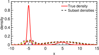
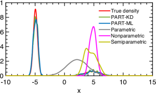
Figure 1: Bimodal posterior combined from 10 subsets. Left: the true posterior and subset posteriors (dashed). Right: aggregated posterior output by various methods compared to the truth. Results are based on 10,000 aggregated samples.

Rare Bernoulli Example

We consider $N=10,000$ Bernoulli trials $x_{i}\overset{\text{iid}}{\sim}\text{Ber}(\theta)$ split into $m=15$ subsets. The parameter $\theta$ is chosen to be $2m/N$ so that on average each subset only contains 2 successes. By random partitioning, the subset posteriors are rather heterogeneous as plotted in dashed lines in the left panel of Figure 9. The prior is set as $\pi(\theta)=\text{Beta}(\theta;2,2)$. The right panel of Figure 9 compares the results of various methods. PART-KD, PART-ML and Weierstrass capture the true posterior shape, while parametric, average and weighted average are all biased. The nonparametric and semiparametric methods produce flat densities near zero (not visible in Figure 9 due to the scale).

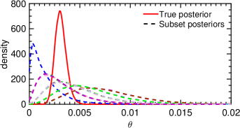
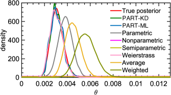
Figure 2: The posterior for the probability $\theta$ of a rare event. Left: the full posterior (solid) and $m=15$ subset posteriors (dashed). Right: aggregated posterior output by various methods. All results are based on 20,000 aggregated samples.

4.2 Bayesian Logistic Regression

Synthetic dataset

The dataset $\{(\mathbf{x}_{i},y_{i})\}_{i=1}^{N}$ consists of $N=50,000$ observations in $p=50$ dimensions. All features $\mathbf{x}_{i}\in\mathbb{R}^{p-1}$ are drawn from $N_{p-1}(\mathbf{0},\mathbf{\Sigma})$ with $p=50$ and $\Sigma_{k,l}=0.9^{|k-l|}$. The model intercept is set to $-3$ and the other coefficient $\bm{\theta}^{\ast}_{j}$’s are drawn randomly from $N(0,5^{2})$. Conditional on $\mathbf{x}_{i}$, $y_{i}\in\{0,1\}$ follows $p(y_{i}=1)=1/(1+\exp(-\bm{\theta}^{\ast T}[1,\mathbf{x}_{i}]))$. The dataset is randomly split into $m=40$ subsets. For both full chain and subset chains, we run adaptive MCMC for 200,000 iterations after 100,000 burn-in. Thinning by 4 results in $T=50,000$ samples.

The samples from the full chain (denoted as $\{\bm{\theta}_{j}\}_{j=1}^{T}$) are treated as the ground truth. To compare the accuracy of different methods, we resample $T$ points $\{\hat{\bm{\theta}}_{j}\}$ from each aggregated posterior and then compare them using the following metrics: (1) RMSE of posterior mean $\|\frac{1}{pT}(\sum_{j}\hat{\bm{\theta}}_{j}-\sum_{j}\bm{\theta}_{j})\|_{2}$ (2) approximate KL divergence $D_{\text{KL}}({p}(\bm{\theta})\|\hat{p}(\bm{\theta}))$ and $D_{\text{KL}}(\hat{p}(\bm{\theta})\|p(\bm{\theta}))$, where $\hat{p}$ and $p$ are both approximated by multivariate Gaussians (3) the posterior concentration ratio, defined as $r=\sqrt{{\sum_{j}\|\hat{\bm{\theta}}_{j}-\bm{\theta}^{\ast}\|_{2}^{2}}/{\sum_{j}\|\bm{\theta}_{j}-\bm{\theta}^{\ast}\|_{2}^{2}}}$, which measures how posterior spreads out around the true value (with $r=1$ being ideal). The result is provided in Table 4. Figure 6 shows the $D_{\text{KL}}(p\|\hat{p})$ versus the length of subset chains supplied to the aggregation algorithm. The results of PART are obtained with $\delta_{\rho}=0.001$, $\delta_{a}=0.0001$ and 40 trees. Figure 4 showcases the aggregated posterior for two parameters in terms of joint and marginal distributions.

Method	RMSE	$D_{\text{KL}}(p\|\hat{p})$	$D_{\text{KL}}(\hat{p}\|p)$	$r$
PART (KD)	0.587	${3.95\times 10^{2}}$	${6.45\times 10^{2}}$	3.94
PART (ML)	1.399	$\mathbf{8.05\times 10^{1}}$	$\mathbf{5.47\times 10^{2}}$	9.17
average	29.93	$2.53\times 10^{3}$	$5.41\times 10^{4}$	184.62
weighted	38.28	$2.60\times 10^{4}$	$2.53\times 10^{5}$	236.15
Weierstrass	6.47	$7.20\times 10^{2}$	$2.62\times 10^{3}$	39.96
parametric	10.07	$2.46\times 10^{3}$	$6.12\times 10^{3}$	62.13
nonparametric	25.59	$3.40\times 10^{4}$	$3.95\times 10^{4}$	157.86
semiparametric	25.45	$2.06\times 10^{4}$	$3.90\times 10^{4}$	156.97

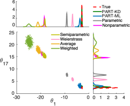
Figure 3: Accuracy of posterior aggregation on logistic regression.

Figure 4: Posterior of $\theta_{1}$ and $\theta_{17}$.

Real datasets

We also run experiments on two real datasets: (1) the Covertype dataset [17] consists of 581,012 observations in 54 dimensions, and the task is to predict the type of forest cover with cartographic measurements; (2) the MiniBooNE dataset [18, 19] consists of 130,065 observations in 50 dimensions, whose task is to distinguish electron neutrinos from muon neutrinos with experimental data. For both datasets, we reserve $1/5$ of the data as the test set. The training set is randomly split into $m=50$ and $m=25$ subsets respectively for covertype and MiniBooNE. Figure 10 shows the prediction accuracy versus total runtime (parallel subset MCMC + aggregation time) for different methods. For each MCMC chain, the first 20% iterations are discarded before aggregation as burn-in. The aggregated chain is required to be of the same length as the subset chains. As a reference, we also plot the result for the full chain and lasso [20] run on the full training set.

[]

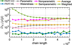
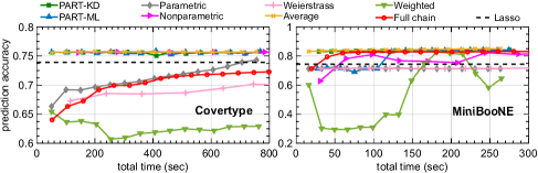
Figure 5: Approximate KL divergence between the full chain and the combined posterior versus the length of subset chains.

[]

Figure 6: Prediction accuracy versus total runtime (running chain + aggregation) on Covertype and MiniBooNE datasets (semiparametric is not compared due to its long running time). Plots against the length of chain are provided in the supplement.

5 Conclusion

In this article, we propose a new embarrassingly-parallel MCMC algorithm PART that can efficiently draw posterior samples for large data sets. PART is simple to implement, efficient in subset combining and has theoretical guarantees. Compared to existing EP-MCMC algorithms, PART has substantially improved performance. Possible future directions include (1) exploring other multi-scale density estimators which share similar properties as partition trees but with a better approximation accuracy (2) developing a tuning procedure for choosing good $\delta_{\rho}$ and $\delta_{a}$, which are essential to the performance of PART.

 

Supplementary Materials

 

Appendix A: Schematic illustration of the algorithm

Here we include a schematic illustration of the density aggregation in PART algorithm.

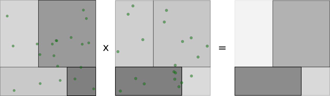
Figure 7: A schematic figure illustrating the density aggregation step of the algorithm. Two trees in the left share the same block structure and the aggregated histogram is obtained by block-wise multiplication and renormalization.

Appendix B: Proof of Theorem 1

Let $\Gamma_{K,\rho}$ be a subset of $\Gamma_{K}$ defined as $\Gamma_{K,\rho}=\big{\{}f_{0}\in\Gamma_{K}|~{}\min_{A_{k}}\mathbbm{E}\bm{1}_{A_{k}}\geq\rho\big{\}}$. We prove a more general form of Theorem 1 here.

Theorem 5.

For any $\delta>0$, if the sample size satisfies that $N>\max\{K,~{}\frac{2\log(2K/\delta)}{\rho(1-c_{0})^{2}}\}$, then with probability at least $1-\delta$, the optimal solution to (8) satisfies that

$$D_{KL}(f\|\hat{f}_{ML})\leq\min_{f_{0}\in\Gamma_{K,\rho}}D_{KL}(f\|f_{0})+C_{\rho}\sqrt{\frac{K}{N}\log\bigg{(}\frac{3eN}{K}\bigg{)}\log\bigg{(}\frac{8}{\delta}\bigg{)}},$$

where $C_{\rho}=48\sqrt{p+1}\max\big{\{}\log D,\log\rho^{-1}\big{\}}$.

Now choosing $\rho=1/K^{1+1/(2p)}$, the condition becomes $N>2(1-c_{0})^{-2}K^{1+1/(2p)}\log(2K/\delta)$, then with probability at least $1-\delta$ we have

$$D_{KL}(f\|\hat{f}_{ML})\leq(C_{1}+2\log K)K^{-\frac{1}{2p}}+C_{2}\max\big{\{}\log D,2\log K\big{\}}\sqrt{\frac{K}{N}\log\bigg{(}\frac{3eN}{K}\bigg{)}\log\bigg{(}\frac{8}{\delta}\bigg{)}},$$

where $C_{1}=2\log D+4pLD$ with $L=\|f^{\prime}\|_{\infty}$ and $C_{2}=48\sqrt{p+1}$.

When multiple densities $f^{(1)}(\theta),\cdots,f^{(m)}(\theta)$ are presented, our goal of imposing the same partition on all functions requires solving a different problem (9). As long as $\mathbbm{\hat{E}}\sum_{i=1}^{m}\hat{f}_{ML}^{(i)}\geq\mathbbm{\hat{E}}\sum_{i=1}^{m}f_{K,\rho}^{(i)}$ remains true, where $f_{K,\rho}^{(i)}=\operatorname*{arg\,min}_{f_{0}\in\Gamma_{K,\rho}}D_{KL}(f^{(i)}\|f_{0})$, the whole proof of Theorem 1 is also valid for (9). Therefore, we have the following Corollary.

Corollary 1 ($m$ copies).

For any $\delta>0$, if the sample size satisfies that $N>2(1-c_{0})^{-2}K^{1+1/(2p)}\log(2mK/\delta)$ and $\rho=1/K^{1+1/(2p)}$, then with probability at least $1-\delta$, the optimal solution to (9) satisfies that

$$\frac{1}{m}\sum_{i=1}^{m}D_{KL}(f^{(i)}\|\hat{f}_{ML}^{(i)}) \leq(C_{1}+2\log K)K^{-\frac{1}{2p}}+C_{2}\max\big{\{}\log D,2\log K\big{\}}\sqrt{\frac{K}{N}\log\bigg{(}\frac{3eN}{K}\bigg{)}\log\bigg{(}\frac{8m}{\delta}\bigg{)}}.$$

To prove Theorem 1 we need the following lemmas.

Lemma 1.

The optimal solution of (8) is also the optimal solution of the following problem,

$$\hat{f}_{ML} =\operatorname*{arg\,max}_{f\in\Gamma_{K}}\frac{1}{N}\sum_{k=1}^{K}n_{k}\log\hat{\pi}_{k},\quad\mbox{s.t. }n_{k}\geq c_{0}\rho N,~{}|A_{k}|\geq\rho/D\mbox{ and }\sum_{k=1}^{K}\hat{\pi}_{k}|A_{k}|=1.$$ (10)

Proof.

We write out the empirical log likelihood

$$\frac{1}{N}\sum_{k=1}^{K}n_{k}\log\hat{\pi}_{k}=\sum_{k=1}^{K}\frac{n_{k}}{N}\log\hat{\pi}_{k}|A_{k}|-\sum_{n_{k}\geq 0}\frac{n_{k}}{N}\log|A_{k}|.$$

For any fixed partition $\{A_{k}\}$, under the constraint that $\sum_{k=1}^{K}\hat{\pi}_{k}|A_{k}|=1$, one can easily see that

$$\hat{\pi}_{k}|A_{k}|=\frac{n_{k}}{N}$$

maximizes the result. ∎

Next, we show that the optimal approximation

$$f_{K,\rho}=\operatorname*{arg\,min}_{\hat{f}_{ML}\in\Gamma_{K,\rho}}D_{KL}(f\|\hat{f}_{ML})$$

is a feasible solution to (10) with a high probability.

Lemma 2.

Let $f_{K,\rho}$ be the optimal approximation in $\Gamma_{K,\rho}$, then $f_{K,\rho}$ satisfies that $\min_{k}|A_{k}|\geq\rho/D$. In addition, with probability at least $1-K\exp(-(1-c_{0})^{2}\rho N/2)$, we have $n_{k}/N\geq c_{0}\rho$, i.e., $f_{K,\rho}$ is a feasible soluton of (10).

Proof.

Let $n_{k}$ be the counts of data points on the partition of $f_{K,\rho}$. Notice $f_{K,\rho}$ is a fixed function that does not depend on the data. Therefore, each $n_{k}$ follows a binomial distribution. Define $P(A_{k})=\mathbbm{E}\bm{1}_{A_{k}}$. According to the definition of $\Gamma_{K,\rho}$, we have $P(A_{k})\geq\rho$. Using the Chernoff’s inequality, we have for any $0<\delta<1$,

$$P\bigg{(}\frac{n_{k}}{N}\leq(1-\delta)P(A_{k})\bigg{)}\leq\exp\bigg{(}-\frac{\delta^{2}NP(A_{k})}{2}\bigg{)}.$$

Taking $\delta=1-c_{0}$ and union bounds we have

$$P\bigg{(}\min_{k}\frac{n_{k}}{N}\geq c_{0}\rho\bigg{)}\geq 1-K\exp(-(1-c_{0})^{2}\rho N/2).$$

On the other hand, the following inequality shows the bound on $|A_{k}|$,

$$|A_{k}|=\int_{A_{k}}1\geq\int_{A_{k}}f/D\geq\rho/D.$$

∎

Lemma 2 states that with a high probability we have $\mathbbm{\hat{E}}\log\hat{f}_{ML}\geq\mathbbm{\hat{E}}\log f_{K,\rho}$. This result will be used to prove our main theorem.

Although the actual partition algorithm selects the dimension for partitioning completely at random for each iteration, in the proof we will assume one predetermined order of partition (such as $\{1,2,3,\cdots,p,1,2,\cdots\}$) just for simplicity. The order of partitioning does not matter as long as every dimension receives sufficient number of partitions. When the selection is randomly taken, with high probability (increasing exponentially with $N$), the number of partitions in each dimension will concentrate around the average. Thus, it suffices to prove the result for the simple $\{1,2,3,\cdots,p,1,2,\cdots\}$ case.

Proof of Theorem 1.

The proof consists of two parts, namely (1) bounding the excess loss compared to the optimal approximation $f_{K,\rho}$ in $\Gamma_{K,\rho}$ and (2) bounding the error between the optimal approximation and the true density.

For the first part, using the fact that $\mathbbm{\hat{E}}\log f_{K,\rho}(\theta)\leq\mathbbm{\hat{E}}\log\hat{f}_{ML}(\theta)$, the excess loss can be expressed as

$$D_{KL}(f\|\hat{f}_{ML}) -D_{KL}(f\|f_{K,\rho})=\mathbbm{E}\log f_{K,\rho}(\theta)-\mathbbm{E}\log\hat{f}_{ML}(\theta)$$

$$=\mathbbm{E}\log f_{K,\rho}(\theta)-\mathbbm{\hat{E}}\log f_{K,\rho}(\theta)+\mathbbm{\hat{E}}\log f_{K,\rho}(\theta)$$

$$\quad-\mathbbm{\hat{E}}\log\hat{f}_{ML}(\theta)+\mathbbm{\hat{E}}\log\hat{f}_{ML}(\theta)-\mathbbm{E}\log\hat{f}_{ML}(\theta)$$

$$\leq\mathbbm{E}\log f_{K,\rho}(\theta)-\mathbbm{\hat{E}}\log f_{K,\rho}(\theta)+\mathbbm{\hat{E}}\log\hat{f}_{ML}(\theta)-\mathbbm{E}\log\hat{f}_{ML}(\theta).$$

Assuming the partitions for $f_{K,\rho}$ and $\hat{f}_{ML}$ are $\{A_{k}\}$ and $\{\hat{A}_{k}\}$ respectively, we have

$$D_{KL}(f\|\hat{f}_{ML}) -D_{KL}(f\|f_{K,\rho})=\sum_{k=1}^{K}\log\pi_{k}\big{(}\mathbbm{E}\bm{1}_{A_{k}}-\mathbbm{\hat{E}}\bm{1}_{A_{k}}\big{)}+\sum_{k=1}^{K}\log\frac{n_{k}}{N|\hat{A}_{k}|}\big{(}\mathbbm{E}\bm{1}_{\hat{A}_{k}}-\mathbbm{\hat{E}}\bm{1}_{\hat{A}_{k}}\big{)}$$

$$\leq\bigg{(}\max_{k}|\log\pi_{k}|+\max_{k}\big{|}\log\frac{n_{k}}{N|\hat{A}_{k}|}\big{|}\bigg{)}\sup_{\{A_{k}\}\in\mathcal{F}_{k}}\sum_{k=1}^{K}|\mathbbm{E}\bm{1}_{A_{k}}-\mathbbm{\hat{E}}\bm{1}_{A_{k}}|.$$ (11)

Following a similar argument as Lemma 1, for $f_{K,\rho}$ we can prove that $\pi_{k}=\int_{A_{k}}f(\theta)d\theta/|A_{k}|$, thus we have $\rho_{0}\leq\pi_{k}\leq D$ for any $1\leq k\leq K$. Similarly for $\frac{n_{k}}{N|A_{k}|}$ we have $\rho\leq\frac{n_{k}}{N|A_{k}|}\leq D/\rho$. Therefore, the first term in (11) can be bounded as

$$\max_{k}|\log\pi_{k}|+\max_{k}\big{|}\log\frac{n_{k}}{N|\hat{A}_{k}|}\big{|}\leq 3\max\{\log D,~{}\log\rho^{-1}\}.$$

The second term in (11) is the concentration of the empirical measure over all possible K-rectangular partitions. Using the result from [chen1987almost], we have the following large deviation inequality. For any $\epsilon\in(0,1)$, we have

$$P\bigg{(}\sup_{\{A_{k}\}\in\mathcal{F}_{k}}\sum_{k=1}^{K}|\mathbbm{E}\bm{1}_{A_{k}}-\mathbbm{\hat{E}}\bm{1}_{A_{k}}|>\epsilon\bigg{)}<4\exp\bigg{\{}-\frac{\epsilon^{2}N}{2^{9}}\bigg{\}},$$ (12)

if $N\geq\max\{K,(100\log 6)/\epsilon^{2},2^{9}(p+1)K\log(3eN/K)/\epsilon^{2}\}$. For any $\delta>0$, taking $\epsilon=2^{9}(p+1)K\log(3eN/K)/N\log(4/\delta)$, we have that

$$\sup_{\{A_{k}\}\in\mathcal{F}_{k}}\sum_{k=1}^{K}|\mathbbm{E}\bm{1}_{A_{k}}-\mathbbm{\hat{E}}\bm{1}_{A_{k}}|\leq 16\sqrt{2(p+1)}\sqrt{\frac{K}{N}\log\bigg{(}\frac{3eN}{K}\bigg{)}\log\bigg{(}\frac{8}{\delta}\bigg{)}},$$

with probability at least $1-\delta/2$. Define $C_{\rho}=48\sqrt{2(p+1)}\max\{\log D,\log\rho^{-1}\}$. When $N>\frac{2\log(2K/\delta)}{\rho(1-c_{0})^{2}}$, Lemma 2 holds with probability at least $1-\delta/2$. Taking the union bound, we have

$$D_{KL}(f\|\hat{f}_{ML})\leq\min_{f_{0}\in\Gamma_{K,\rho}}D_{KL}(f\|f_{0})+C_{\rho}\sqrt{\frac{K}{N}\log\bigg{(}\frac{3eN}{K}\bigg{)}\log\bigg{(}\frac{8}{\delta}\bigg{)}}$$ (13)

holds with probability greater than $1-\delta$.

To prove the second part, we construct one reference density $\tilde{f}\in\Gamma_{K,\rho}$ that gives the error specified in the theorem. According to the argument provided in the paragraph prior to this proof, we assume the dimension that we cut at each iteration follows an order $\{1,2,\cdots,p,1,2,\cdots\}$. We then construct $f_{0}$ in the following way. At iteration $i$, we check the probability on the whole region.

• If the probability is greater than $2\rho$, we then cut at the midpoint of the selected dimension. If the resulting two blocks $B_{1}$ and $B_{2}$ satisfy that $P_{f}(B_{1})\geq\rho$ and $P_{f}(B_{2})\geq\rho$, we continue to the next iteration. However, if any of them fails to satisfy the condition, we find the minimum-deviated cut that satisfies the probability requirement.

• If the probability on the whole region is less than $2\rho$, we stop cutting on this region and move to the next region for the current iteration.

It is easy to show that as long as $\rho\leq 1/(2K)$, the above procedure is able to yield a $K$-block partition $\{\tilde{A}_{k}\}$ before termination. Finally, the reference density $\tilde{f}$ is defined as

$$\tilde{f}(\theta)=\sum_{k=1}^{K}\frac{\int_{\tilde{A}_{k}}f(\theta)d\theta}{|\tilde{A}_{k}|}\operatorname{1}_{\tilde{A}_{k}}(\theta).$$ (14)

The construction procedure ensures the following property for $\tilde{f}\in\Gamma_{K,\rho}$. Assuming $K\in[2^{d},2^{d+1})$ for some $d>0$, then each $\tilde{A}_{k}$ must fall into either of the following two categories (could be both),

1. $\rho\leq P_{f}(\tilde{A}_{k})\leq 2\rho$,

2. $P_{f}(\tilde{A}_{k})\geq\rho$ and the longest edge of cube $\tilde{A}_{k}$ must be less than $2^{-\lfloor d/p\rfloor}\leq 2^{-d/p+1}\leq 4k^{-1/p}$.

We use $I_{1}$ and $I_{2}$ to denote the two different collections of sets. Now for any $b_{0}>0$, let $B=\{f<b_{0}\}\cup\{\tilde{f}<b_{0}\}$. We divide the KL-divergence between $f$ and $\tilde{f}$ into three regions and bound them accordingly.

$$D_{KL}(f\|\tilde{f})=\int_{\Omega}f\log\frac{f}{\tilde{f}} =\int_{B}f\log\frac{f}{\tilde{f}}+\int_{B^{c}\cap\big{(}\bigcup I_{1}\big{)}}f\log\frac{f}{\tilde{f}}+\int_{B^{c}\cap\big{(}\bigcup I_{2}\big{)}}f\log\frac{f}{\tilde{f}}$$

$$=M_{1}+M_{2}+M_{3}.$$

We first look at $M_{1}$. Because $\tilde{f}$ is a block-valued function, $\{\tilde{f}<b_{0}\}$ must be the union of all the $\tilde{A}_{k}$ that satisfies $\int_{\tilde{A}_{k}}f(\theta)d\theta\leq b_{0}|\tilde{A}_{k}|$. Therefore, we have

$$\int_{\tilde{f}<b_{0}}f(\theta)d\theta=\sum_{\tilde{A}_{k}:~{}\int_{\tilde{A}_{k}}f(\theta)d\theta\leq b_{0}|\tilde{A}_{k}|}\int_{\tilde{A}_{k}}f(\theta)d\theta\leq\sum_{\tilde{A}_{k}:~{}\int_{\tilde{A}_{k}}f(\theta)d\theta\leq b_{0}|\tilde{A}_{k}|}b_{0}|\tilde{A}_{k}|\leq b_{0}.$$

Therefore, we have

$$\int_{B}f(\theta)d\theta\leq\int_{\tilde{f}<b_{0}}f(\theta)d\theta+\int_{f<b_{0}}f(\theta)d\theta=b_{0}+b_{0}|\Omega|=2b_{0}.$$

Because $\tilde{f}\geq\min_{k}P(A_{k})/|A_{k}|\geq P(A_{k})\geq\rho$, we have

$$M_{1}=\int_{B}f\log\frac{f}{\tilde{f}}\leq\int_{B}f(\theta)\log\frac{b_{0}}{\rho}\leq 2b_{0}\big{|}\log\frac{b_{0}}{\rho}\big{|}.$$

Next, we look at $M_{2}$. It is clear that

$$\int_{B^{c}\cap\big{(}\bigcup I_{1}\big{)}}f(\theta)d\theta\leq\int_{\big{(}\bigcup I_{1}\big{)}}f(\theta)d\theta\leq card(I_{1})2\rho,$$

and hence we have

$$M_{2}=\int_{B^{c}\cap\big{(}\bigcup I_{1}\big{)}}f\log\frac{f}{\tilde{f}}\leq\int_{B^{c}\cap\big{(}\bigcup I_{1}\big{)}}f(\theta)\log\frac{D}{b_{0}}\leq card(I_{1})2\rho\big{|}\log\frac{D}{b_{0}}\big{|}\leq 2K\rho\big{|}\log\frac{D}{b_{0}}\big{|}.$$

Now for $M_{3}$, we first use the inequality that $\log x\leq x-1$ for any $x>0$,

$$M_{3}=\int_{B^{c}\cap\big{(}\bigcup I_{2}\big{)}}f\log\frac{f}{\tilde{f}}\leq\int_{B^{c}\cap\big{(}\bigcup I_{2}\big{)}}f\bigg{(}\frac{f}{\tilde{f}}-1\bigg{)}\leq\int_{B^{c}\cap\big{(}\bigcup I_{2}\big{)}}\frac{f}{\tilde{f}}(f-\tilde{f})\leq\frac{D}{b_{0}}\int_{\bigcup I_{2}}|f-\tilde{f}|.$$

Using the mean value theorem for integration, we have $\int_{\tilde{A}_{k}}f(\theta)/|\tilde{A}_{k}|=f(\theta_{0})$ for some $\theta_{0}\in\tilde{A}_{k}$. Also because $f\in C^{1}(\Omega)$, $\|f^{\prime}\|_{\infty}$ is bounded, i.e., there exists some constant $L$ such that $|f(x_{1})-f(x_{2})|\leq L\sum_{j=1}^{p}|x_{1j}-x_{2j}|$. Therefore, we have

$$\int_{\bigcup I_{2}}|f-\tilde{f}|=\sum_{\tilde{A}_{k}\in I_{2}}\int_{\tilde{A}_{k}}|f(\theta)-\tilde{f}(\theta)|=\sum_{\tilde{A}_{k}\in I_{2}}\int_{\tilde{A}_{k}}|f(\theta)-f(\theta_{0})|\leq\sum_{\tilde{A}_{k}\in I_{2}}4pLk^{-\frac{1}{p}}|\tilde{A}_{k}|\leq 4pLk^{-\frac{1}{p}},$$

and thus

$$M_{3}\leq\frac{4pLD}{b_{0}}K^{-\frac{1}{p}}.$$

Putting all pieces together we have

$$D_{KL}(f\|\tilde{f})\leq 2b_{0}\big{|}\log\frac{b_{0}}{\rho}\big{|}+2K\rho\big{|}\log\frac{D}{b_{0}}\big{|}+\frac{4pLD}{b_{0}}K^{-\frac{1}{p}}.$$

Now taking $b_{0}=K^{-1/(2p)}$ and $\rho=K^{-1-1/(2p)}$, we have

$$D_{KL}(f\|\tilde{f}) \leq(\log K)K^{-\frac{1}{2p}}+2(\log D+\frac{\log K}{2p})K^{-\frac{1}{2p}}+4pLDK^{-\frac{1}{2p}}$$

$$\leq(2\log K+2\log D+4pLD)K^{-\frac{1}{2p}}.$$

Now defining $C_{1}=2\log D+4pLD$ and $C_{2}=48\sqrt{p+1}$ and combining with (13), we have

$$D_{KL}(f\|\hat{f}_{ML})\leq(C_{1}+2\log K)K^{-\frac{1}{2p}}+C_{2}\max\big{\{}\log D,2\log K\big{\}}\sqrt{\frac{K}{N}\log\bigg{(}\frac{3eN}{K}\bigg{)}\log\bigg{(}\frac{8}{\delta}\bigg{)}}.$$

∎

Appendix C: Proof of Theorem 2

The KD-tree $\hat{f}_{KD}$ always cuts at the empirical median for different dimensions, aiming to approximate the true density by equal probability partitioning. For $\hat{f}_{KD}$ we have the following result.

Theorem 6.

For any $\varepsilon>0$, define $r_{\varepsilon}=\log_{2}\bigg{(}1+\frac{1}{2+3L/\varepsilon}\bigg{)}$. For any $\delta>0$, if $N>32e^{2}(\log K)^{2}K\log(2K/\delta)$, then with probability at least $1-\delta$, we have

$$\|\hat{f}_{KD}-f_{KD}\|_{1}\leq\varepsilon+pLK^{-\frac{r_{\varepsilon}}{p}}+4e\log K\sqrt{\frac{2K}{N}\log\bigg{(}\frac{2K}{\delta}\bigg{)}}.$$

If the function is further lower bounded by some constant $b_{0}>0$, we can then obtain an upper bound on the KL-divergence. Define $r_{b_{0}}=\log_{2}\bigg{(}1+\frac{1}{2+3L/b_{0}}\bigg{)}$ and we have

$$D_{KL}(f\|\hat{f}_{KD})\leq\frac{pLD}{b_{0}}K^{-\frac{r_{b_{0}}}{p}}+8e\log K\sqrt{\frac{2K}{N}\log\bigg{(}\frac{2K}{\delta}\bigg{)}}.$$

When there are multiple functions and the median partition is performed on pooled data, the partition might not happen at the empirical median on each subset. However, as long as the partition quantiles are upper and lower bounded by $\alpha$ and $1-\alpha$ for some $\alpha\in[1/2,1)$, we can establish similar theory as Theorem 2.

Corollary 2.

Assume we instead partition at different quantiles that are upper and lower bounded by $\alpha$ and $1-\alpha$ for some $\alpha\in[1/2,1)$. Define $r_{\varepsilon}=\log_{2}\bigg{(}1+\frac{(1-\alpha)}{2\alpha+3L/\varepsilon+1}\bigg{)}$ and $r_{b_{0}}=\log_{2}\bigg{(}1+\frac{(1-\alpha)}{2\alpha+3L/b_{0}+1}\bigg{)}$. For any $\delta>0$, if $N>\frac{12e^{2}}{(1-\alpha)^{2}}K(\log K)^{2}\log(K/\delta)$, then with probability at least $1-\delta$ we have

$$\|\hat{f}_{KD}-f_{KD}\|_{1}\leq\varepsilon+pLK^{-\frac{r_{\varepsilon}}{p}}+\frac{2e\log K}{1-\alpha}K^{1-\log_{2}\alpha^{-1}}\sqrt{\frac{3K}{N}\log\bigg{(}\frac{2K}{\delta}\bigg{)}}$$

and if the function is lower bounded by $b_{0}$, then we have

$$D_{KL}(f\|\hat{f}_{KD})\leq\frac{pLD}{b_{0}}K^{-\frac{r_{b_{0}}}{p}}+\frac{4e\log K}{1-\alpha}K^{1-\log_{2}\alpha^{-1}}\sqrt{\frac{3K}{N}\log\bigg{(}\frac{2K}{\delta}\bigg{)}}.$$

Following the same argument for Theorem 1, we will prove Theorem 2 by assuming a predetermined order of partition (such as $\{1,2,3,\cdots,p,1,2,\cdots\}$) for simplicity, though in the actual precedure, the dimensions are selected completely at random. We need the following two lemmas to prove Theorem 2. Let $f_{KD}$ have the same partition as $\hat{f}_{KD}$ but with function value replaced by the true probability on each region divided by the area, i.e., $f_{KD}=\sum_{A_{k}}\frac{\int_{A_{k}}f(\theta)d\theta}{|A_{k}|}\operatorname{1}_{A_{k}}(\theta)$.

Lemma 3.

With $f_{KD}$ defined above, for any $\delta>0$, if $N>32e^{2}(\log K)^{2}K\log(K/\delta)$, then with probability at least $1-\delta$, we have

$$\|\hat{f}_{KD}-f_{KD}\|_{1}\leq 4e\log K\sqrt{\frac{2K}{N}\log\bigg{(}\frac{K}{\delta}\bigg{)}}$$

and

$$D_{KL}(f\|\hat{f}_{KD})\leq D_{KL}(f\|f_{KD})+8e\log K\sqrt{\frac{2K}{N}\log\bigg{(}\frac{K}{\delta}\bigg{)}}.$$

If we instead partition at some different quantiles, which are upper bounded by $\alpha$ and lower bounded by $1-\alpha$ for some $\alpha\in[1/2,1)$, then for any $\delta>0$, if $N>\frac{12e^{2}}{(1-\alpha)^{2}}K(\log K)^{2}\log(K/\delta)$, with probability at least $1-\delta$ we have

$$\|\hat{f}_{KD}-f_{KD}\|_{1}\leq\frac{2e\log K}{1-\alpha}K^{1-\log_{2}\alpha^{-1}}\sqrt{\frac{3K}{N}\log\bigg{(}\frac{K}{\delta}\bigg{)}},$$

and

$$D_{KL}(f\|\hat{f}_{KD})\leq D_{KL}(f\|f_{KD})+\frac{4e\log K}{1-\alpha}K^{1-\log_{2}\alpha^{-1}}\sqrt{\frac{3K}{N}\log\bigg{(}\frac{K}{\delta}\bigg{)}}.$$

Proof.

The proof is based on how close the data median is to the true median. Suppose there are $N_{i}$ points in the current region, condition on this region, and partition it into two regions $\hat{A}_{1}$ and $\hat{A}_{2}$ by cutting at the data median point $\hat{M}_{i}$. Denote the true median by $M_{i}$ and two anchor points $M_{i}-\epsilon_{1}$, $M_{i}+\epsilon_{2}$ such that $P(X\leq M_{i}-\epsilon_{1})=1/2-t$ and $P(X\leq M_{i}+\epsilon_{2})=1/2+t$ for some $0<t<1/2$. By Chernoff’s inequality we have

$$P(\hat{M}_{i}\leq M_{i}-\epsilon_{1})\leq\exp\bigg{\{}-\frac{t^{2}N_{i}}{1+2t}\bigg{\}}$$

and

$$P(\hat{M}_{i}\geq M_{i}+\epsilon_{2})\leq\exp\bigg{\{}-\frac{t^{2}N_{i}}{1+2t}\bigg{\}}.$$

The above two inequalities indicate that with high probability $\hat{M}_{i}$ is within the interval $(M_{i}-\epsilon_{1},M_{i}+\epsilon_{2})$. Therefore, the probabilities on $A_{1}$ and $A_{2}$ also satisfy that

$$P\bigg{(}\big{|}\mathbbm{E}\bm{1}_{A_{i}}-\frac{1}{2}\big{|}\geq t\bigg{)}\leq\exp\bigg{\{}-\frac{t^{2}N_{i}}{1+2t}\bigg{\}}.$$ (15)

Now consider the $K$ regions of $\hat{f}_{KD}$ and $f_{KD}$. Each partition will bring an error of at most $1/2+t$ to the estimation of the region probability. Therefore, assuming $K\in[2^{d}+1,2^{d+1})$ we have for each region $A_{k}$ ($A_{k}$ is a random variable) that

$$\bigg{(}\frac{1}{2}-t\bigg{)}^{d}\leq\int_{A_{k}}f(\theta)d\theta\leq\bigg{(}\frac{1}{2}+t\bigg{)}^{d}$$

if $n_{k}/N=1/2^{d}$, or

$$\bigg{(}\frac{1}{2}-t\bigg{)}^{d+1}\leq\int_{A_{k}}f(\theta)d\theta\leq\bigg{(}\frac{1}{2}+t\bigg{)}^{d+1},$$

if $n_{k}/N=1/2^{d+1}$. Notice that for all iterations before the current partition, we always have $N_{i}\geq N/K$. Therefore the probability is guaranteed to be greater than $1-K\exp\bigg{\{}-\frac{t^{2}N/K}{1+2t}\bigg{\}}$. The above result indicates that

$$\max_{A_{k}}\bigg{|}\int_{A_{k}}f_{KD}(\theta) -\int_{A_{k}}\hat{f}_{KD}(\theta)\bigg{|}\leq\max\bigg{\{}\bigg{(}\frac{1}{2}+t\bigg{)}^{d+1}-\bigg{(}\frac{1}{2}\bigg{)}^{d+1},-\bigg{(}\frac{1}{2}-t\bigg{)}^{d+1}+\bigg{(}\frac{1}{2}\bigg{)}^{d+1}\bigg{\}}$$

$$=\bigg{(}\frac{1}{2}\bigg{)}^{d+1}\max\bigg{\{}(1+2t)^{d+1}-1,1-(1-2t)^{d+1}\bigg{\}}$$

$$=\bigg{(}\frac{1}{2}\bigg{)}^{d+1}\bigg{(}(d+1)(1+2\tilde{t})^{d}2t\bigg{)},$$

where $\tilde{t}\in(0,t)$. So if $t<1/(2d)$, then $(1+2\tilde{t})^{d}\leq(1+1/d)^{d}<e$ and we have

$$\max_{A_{k}}\bigg{|}\int_{A_{k}}f_{KD}(\theta) -\int_{A_{k}}\hat{f}_{KD}(\theta)\bigg{|}\leq 2(d+1)e\bigg{(}\frac{1}{2}\bigg{)}^{d+1}t\leq\frac{4et\log K}{K}.$$ (16)

This result implies that the total variation distance satisfies that

$$\|\hat{f}_{KD}-f_{KD}\|_{1}=\sum_{k}\int_{A_{k}}|\hat{f}_{KD}(\theta)-f_{KD}(\theta)|=\sum_{k}\bigg{|}\int_{A_{k}}\hat{f}_{KD}(\theta)-\int_{A_{k}}f_{KD}(\theta)\bigg{|}\leq 4et\log K.$$

Similarly, one can also prove that

$$\max_{A_{k}}\bigg{|}\frac{\int_{A_{k}}f_{KD}(\theta)}{\int_{A_{k}}\hat{f}_{KD}(\theta)}-1\bigg{|}\leq\max_{A_{k}}\bigg{|}\frac{\int_{A_{k}}f_{KD}(\theta)-\int_{A_{k}}\hat{f}_{KD}(\theta)}{\int_{A_{k}}\hat{f}_{KD}(\theta)}\bigg{|}\leq 4et\log K.$$

Denote $\int_{A_{k}}f(\theta)=\int_{A_{k}}f_{KD}(\theta)$ by $P(A_{k})$ and $\int_{A_{K}}\hat{f}_{KD}f(\theta)$ by $\hat{P}(A_{k})$. The KL-divergence can then be computed as

$$D_{KL}(f\|\hat{f}_{KD}) -D_{KL}(f\|f_{KD})=\sum_{A_{k}}\int_{A_{k}}f(\theta)(\log f_{KD}(\theta)-\log\hat{f}_{KD}(\theta))$$

$$=\sum_{A_{k}}\int_{A_{k}}f(\theta)\bigg{(}\log\int_{A_{k}}f(\theta)-\log\int_{A_{k}}\hat{f}_{KD}(\theta)\bigg{)}$$

$$=\sum_{A_{k}}P(A_{k})\bigg{(}\log\frac{P(A_{k})}{\hat{P}(A_{k})}\bigg{)}\leq\sum_{A_{k}}P(A_{k})\bigg{(}\frac{P(A_{k})}{\hat{P}(A_{k})}-1\bigg{)}$$

$$=\sum_{A_{k}}\frac{P(A_{k})}{\hat{P}(A_{k})}\bigg{(}P(A_{k})-\hat{P}(A_{k})\bigg{)}$$

$$\leq(1+4et\log K)4et\log K\leq 8et\log K,$$

as long as $t<\min\bigg{\{}\frac{1}{4e\log K},\frac{1}{2\log_{2}K}\bigg{\}}$, with probability at least $1-K\exp\bigg{\{}-\frac{t^{2}N}{2K}\bigg{\}}$. Consequently, for any $\delta>0$, if $N>32e^{2}K(\log K)^{2}\log(K/\delta)$, then with probability at least $1-\delta$, we have

$$\|\hat{f}_{KD}-f_{KD}\|_{1}\leq 4e\log K\sqrt{\frac{2K}{N}\log\bigg{(}\frac{K}{\delta}\bigg{)}}$$

and

$$D_{KL}(f\|\hat{f}_{KD})\leq D_{KL}(f\|f_{KD})+8e\log K\sqrt{\frac{2K}{N}\log\bigg{(}\frac{K}{\delta}\bigg{)}}.$$

When the partition occurs at a different quantile, which is assumed to be $\alpha_{i}$ for iteration $i$, we have

$$\prod_{i=1}^{d+1}(\alpha_{i}^{\prime}-t)\leq\int_{A_{k}}f(\theta)d\theta\leq\prod_{i=1}^{d+1}(\alpha_{i}^{\prime}+t),$$

where $\alpha_{i}^{\prime}=\alpha_{i}$ if $A_{k}$ takes the region containing smaller data values and $\alpha_{i}^{\prime}=1-\alpha_{i}$ if $A_{k}$ takes the other half. First, (15) can be updated as

$$P\bigg{(}\big{|}\mathbbm{E}\operatorname{1}_{A_{i}}-\alpha_{i}^{\prime}\big{|}\geq t\bigg{)}\leq\exp\bigg{\{}-\frac{t^{2}N_{i}}{3\alpha}\bigg{\}}\leq\exp\bigg{\{}-\frac{t^{2}N_{i}}{3}\bigg{\}},$$ (17)

if $t<1-\alpha$. Then we can bound the difference between $\int_{A_{k}}f(\theta)$ and $\int_{A_{k}}\hat{f}_{KD}(\theta)$ as

$$\max_{A_{k}}\bigg{|}\int_{A_{k}}f_{KD}(\theta) -\int_{A_{k}}\hat{f}_{KD}(\theta)\bigg{|}\leq\max\bigg{\{}\prod_{i=1}^{d+1}(\alpha_{i}^{\prime}+t)-\prod_{i=1}^{d+1}\alpha_{i}^{\prime},~{}-\prod_{i=1}^{d+1}(\alpha_{i}^{\prime}-t)+\prod_{i=1}^{d+1}\alpha_{i}^{\prime}\bigg{\}}$$

$$\leq\max\bigg{[}\prod_{i=1}^{d+1}\alpha_{i}^{\prime}\bigg{\{}\prod_{i=1}^{d+1}\bigg{(}1+\frac{t}{\alpha_{i}^{\prime}}\bigg{)}-1\bigg{\}},~{}\prod_{i=1}^{d+1}\alpha_{i}^{\prime}\bigg{\{}1-\prod_{i=1}^{d+1}\bigg{(}1-\frac{t}{\alpha_{i}^{\prime}}\bigg{)}\bigg{\}}\bigg{]}$$

$$\leq\prod_{i=1}^{d+1}\alpha_{i}^{\prime}\cdot(d+1)\bigg{(}1+\frac{\tilde{t}}{1-\alpha}\bigg{)}^{d}\frac{t}{1-\alpha},$$

where $\tilde{t}\in(0,t)$. Thus if $t<(1-\alpha)/d$, then we have

$$\max_{A_{k}}\bigg{|}\int_{A_{k}}f_{KD}(\theta) -\int_{A_{k}}\hat{f}_{KD}(\theta)\bigg{|}\leq\frac{e(d+1)t\alpha^{d+1}}{1-\alpha}\leq\frac{2et\log K}{(1-\alpha)K^{\log_{2}\alpha^{-1}}},$$

and

$$\max_{A_{k}}\bigg{|}\frac{\int_{A_{k}}f_{KD}(\theta)}{\int_{A_{k}}\hat{f}_{KD}(\theta)}-1\bigg{|}\leq\frac{2et\log K}{1-\alpha}.$$

The total variation distance follows

$$\|\hat{f}_{KD}-f_{KD}\|_{1}\leq K\cdot\frac{2et\log K}{(1-\alpha)K^{\log_{2}\alpha^{-1}}}=\frac{2et\log K}{1-\alpha}K^{1-\log_{2}\alpha^{-1}},$$

and the KL-divergence follows

$$D_{KL}(f\|\hat{f}_{KD}) -D_{KL}(f\|f_{KD})\leq\bigg{(}1+\frac{2et\log K}{1-\alpha}\bigg{)}\frac{2et\log K}{1-\alpha}K^{1-\log_{2}\alpha^{-1}}\leq\frac{4et\log K}{1-\alpha}K^{1-\log_{2}\alpha^{-1}},$$

if $t<1/(2e(1-\alpha)\log K)$. Consequently, for any $\delta>0$, if $N>\frac{12e^{2}}{(1-\alpha)^{2}}K(\log K)^{2}\log(K/\delta)$, then with probability at least $1-\delta$, we have

$$\|\hat{f}_{KD}-f_{KD}\|_{1}\leq\frac{2e\log K}{1-\alpha}K^{1-\log_{2}\alpha^{-1}}\sqrt{\frac{3K}{N}\log\bigg{(}\frac{K}{\delta}\bigg{)}},$$

and

$$D_{KL}(f\|\hat{f}_{KD})\leq D_{KL}(f\|f_{KD})+\frac{4e\log K}{1-\alpha}K^{1-\log_{2}\alpha^{-1}}\sqrt{\frac{3K}{N}\log\bigg{(}\frac{K}{\delta}\bigg{)}}.$$

∎

Our next result is to bound the distance between $f_{KD}$ and the true density $f$. Again, the proof depends on the control of the smallest value of $f$ and the longest edge of every block. One issue now is that each partition might not happen at the midpoint, but it should not deviate from the midpoint too much given the bound on the $f^{\prime}$, i.e., we have the following proposition.

Proposition 1.

Assume we aim to partition an edge of length $h$ (on dimension $q$) of a rectangular region $A$, which has a probability of $P$ and an area of $|A|$. We distinguish the resulting two regions as the left and the right region and the corresponding edges (on dimension $q$) as $h_{\text{left}}$ and $h_{\text{right}}$ (i.e., $h_{\text{left}}+h_{\text{right}}=h$). Suppose the partition ensures that the left region has probability of $\gamma P$, where $\gamma\geq 1/2$. If $\|f^{\prime}\|_{\infty}\leq L$, then the longer edge $h^{*}=\max\{h_{\text{left}},h_{\text{right}}\}$ satisfies that

$$\frac{h^{*}}{h}\leq 1-\frac{1-\gamma}{1+Lh\frac{|A|}{P}}.$$

Proof.

It suffices to bound $h_{\text{left}}$ as $\gamma>1-\gamma$. Let $g(t)=\int_{x:(t,x)\in A}f(t,x)$, where $t$ represents the variable of dimension $q$ and $x$ stands for the other dimensions. We then have $\int_{t:h}g(t)=P$, $\int_{x:(t,x)\in A}1dx=|A|/h$ and

$$|g(t_{1})-g(t_{2})|\leq\int_{x:(t,x)}(f(t_{1},x)-f(t_{2},x))\leq L|t_{1}-t_{2}||A|/h.$$

Therefore, using the mean value theorem for the integration, we know that

$$\bigg{|}\frac{\int_{t:h_{\text{left}}}g(t)}{h_{\text{left}}}-\frac{\int_{t:h_{\text{right}}}g(t)}{h_{\text{right}}}\bigg{|}\leq L|A|,$$

which implies that

$$\bigg{|}\frac{\gamma h}{h_{\text{left}}}-\frac{(1-\gamma)h}{h_{\text{right}}}\bigg{|}\leq\frac{L|A|h}{P}.$$

Now if we solve the following inequality

$$|\gamma/a-(1-\gamma)/b|\leq c\quad\mbox{and}\quad a+b=1,a\geq 0,b\geq 0,$$

with some simple algebra we can get

$$a\leq 1-\frac{1-\gamma}{1+c}.$$

Plug in the corresponding value, we have

$$\frac{h_{\text{left}}}{h}\leq 1-\frac{1-\gamma}{1+Lh\frac{|A|}{P}}.$$

∎

With Proposition 1, we can now obtain the upper bound for $\|f-f_{KD}\|_{1}$ and $D_{KL}(f\|f_{KD})$.

Lemma 4.

For any $\varepsilon>0$, define $r_{\varepsilon}=\log_{2}\bigg{(}1+\frac{1}{2+3L/\varepsilon}\bigg{)}$. If $N\geq 72K\log(K/\delta)$ for any $\delta>0$, then with probability at least $1-\delta$, we have

$$\|f-f_{KD}\|_{1}\leq\varepsilon+pLK^{-\frac{r_{\varepsilon}}{p}}.$$

If the $f$ is further lower bounded by some $b_{0}>0$, the KL-divergence can be bounded as

$$D_{KL}(f\|f_{KD})\leq\frac{pLD}{b_{0}}K^{-\frac{r_{b_{0}}}{p}},$$

where $r_{b_{0}}=\log_{2}\bigg{(}1+\frac{1}{2+3L/b_{0}}\bigg{)}$.

Now suppose we instead partition at different quantiles, upper and lower bounded by $\alpha$ and $1-\alpha$ for some $\alpha\in(1/2,1)$. For any $\delta>0$, if $N\geq\frac{27}{(1-\alpha)^{2}}K\log(K/\delta)$ then the above two bounds hold with different $r_{\varepsilon}$ and $r_{b_{0}}$ as

$$r_{\varepsilon}=\log_{2}\bigg{(}1+\frac{(1-\alpha)}{2\alpha+3L/\varepsilon+1}\bigg{)}\quad\mbox{and}\quad r_{b_{0}}=\log_{2}\bigg{(}1+\frac{(1-\alpha)}{2\alpha+3L/b_{0}+1}\bigg{)}.$$

Proof.

The proof for the total variation distance follows similarly as Theorem 1. For any $\varepsilon>0$, we consider $B=\{f_{KD}<\varepsilon/2\}$. We then partition the total variation distance formula into two parts

$$\|f_{KD}-f\|_{1}=\int_{B}|f_{KD}-f|+\int_{B^{c}}|f_{KD}-f|=M_{1}+M_{2}.$$

It is straightforward to bound $M_{1}$. $B$ is a union of $A_{k}$’s which satisfies $\int_{A_{k}}f(\theta)\leq\varepsilon|A_{k}|/2$. Therefore,

$$M_{1}\leq\int_{B}f+\int_{B}f_{KD}=\sum_{A_{k}:\cup A_{k}=B}2\int_{A_{k}}f(\theta)\leq\varepsilon.$$

Now for $M_{2}$, the usual analysis shows that our result depends on the longest edge of each block, i.e.,

$$M_{2}=\int_{B^{c}}|f_{KD}-f|=\sum_{A_{k}:\cup A_{k}=B^{c}}\int_{A_{k}}|f_{KD}-f|\leq\sum_{A_{k}:\cup A_{k}=B^{c}}pLh^{*}_{k}|A_{k}|=pL|B^{c}|\max_{A_{k}}h^{*}_{k}\leq pL\max_{A_{k}}h^{*}_{k},$$

where $h^{*}_{k}$ is the longest edge of each block contained in $B^{c}$. Now using Proposition 1, we know for iteration $i$ the partitioned edge at each block follows

$$h_{i}\leq\bigg{(}1-\frac{1-\gamma}{1+Lh\frac{|A|}{P}}\bigg{)}h_{i-1}\leq\bigg{(}1-\frac{1-\gamma}{1+L/\varepsilon}\bigg{)}h_{i-1}.$$

When $K\in(2^{d},2^{d+1}]$, each dimension receives $\lfloor d/p\rfloor$ stages of partitioning; therefore, we have for each block, the longest edge satisfies that

$$h^{*}\leq\bigg{(}1-\frac{1-\gamma}{1+L/\varepsilon}\bigg{)}^{\frac{\log_{2}K}{p}}\leq K^{-\frac{r_{\varepsilon}}{p}},$$

where $r_{\varepsilon}=\log_{2}\bigg{(}1+\frac{(1-\gamma)}{\gamma+L/\varepsilon}\bigg{)}$. This implies

$$M_{2}\leq pLK^{-\frac{r_{\varepsilon}}{p}}\quad\mbox{and}\quad\|f_{KD}-f\|_{1}\leq\varepsilon+pLK^{-\frac{r_{\varepsilon}}{p}}.$$

Now, according to (15), we know with probability at least $1-K\exp\{-t^{2}N/(2K)\}$,

$$\gamma\leq\frac{1}{2}+t.$$

Taking $t=1/6$, we get

$$r_{\varepsilon}=\log_{2}\bigg{(}1+\frac{1}{2+3L/\varepsilon}\bigg{)},$$

with probability at least $1-K\exp\{-N/(72K)\}$. So if $N>72K\log(K/\delta)$, then the probability is at least $1-\delta$. For the case when $\gamma=\alpha+t$, we choose $t=(1-\alpha)/3$, then

$$r_{\varepsilon}=\log_{2}\bigg{(}1+\frac{(1-\alpha)}{2\alpha+3L/\varepsilon+1}\bigg{)}$$

with probability at least $1-\delta$ if $N>\frac{27}{(1-\alpha)^{2}}K\log(K/\delta)$.

For KL-divergence, if $f$ is lower bounded by some constant $b_{0}>0$, then we know that

$$D_{KL}(f\|f_{KD}) =\int_{\Omega}f(\theta)\log\frac{f(\theta)}{f_{KD}(\theta)}\leq\int_{\Omega}f(\theta)\bigg{(}\frac{f(\theta)}{f_{KD}(\theta)}-1\bigg{)}$$

$$\leq\max_{\theta}\frac{f(\theta)}{f_{KD}(\theta)}\int_{\Omega}|f(\theta)-f_{KD}(\theta)|\leq\frac{D}{b_{0}}\|f-f_{KD}\|_{1}.$$

Because $f$ and $f_{KD}$ are both lower bounded by $b_{0}$, we can follow the proof for $\|f-f_{KD}\|_{1}$ with $\varepsilon=b_{0}$ and ignore $M_{1}$. Thus we have

$$D_{KL}(f\|f_{KD})\leq\frac{pLD}{b_{0}}K^{-\frac{r_{b_{0}}}{p}},$$

where $r_{b_{0}}=\log_{2}\bigg{(}1+\frac{(1-\gamma)}{\gamma+L/b_{0}}\bigg{)}$. Similarly, if we take $\gamma=2/3$ and $N\geq 72K\log(K/\delta)$, then with probability at least $1-\delta$, we have

$$r_{b_{0}}=\log_{2}\bigg{(}1+\frac{1}{2+3L/b_{0}}\bigg{)}.$$

If we take $\gamma=(2\alpha+1)/3$ and $N>\frac{27}{(1-\alpha)^{2}}K\log(K/\delta)$, then with probability at least $1-\delta$, we have

$$r_{b_{0}}=\log_{2}\bigg{(}1+\frac{(1-\alpha)}{2\alpha+3L/b_{0}+1}\bigg{)}.$$

∎

Theorem 2 and Corollary 2 follow directly from Lemma 3 and 4.

Proof of Theorem 2 and Corollary 2.

For any $\varepsilon>0$, define $r_{\varepsilon}$ and $r_{b_{0}}$ as in Lemma 4. Thus, for any $\delta>0$, if $N>32e^{2}(\log K)^{2}K\log\frac{2K}{\delta}$, then with probability $1-\delta/2$ we have

$$\|\hat{f}_{KD}-f_{KD}\|_{1}\leq 4e\log K\sqrt{\frac{2K}{N}\log\bigg{(}\frac{2K}{\delta}\bigg{)}}$$

and

$$D_{KL}(f\|\hat{f}_{KD})\leq D_{KL}(f\|f_{KD})+8e\log K\sqrt{\frac{2K}{N}\log\bigg{(}\frac{2K}{\delta}\bigg{)}}.$$

Also, with probability $1-\delta/2$ we have

$$\|f-f_{KD}\|_{1}\leq\varepsilon+pLK^{-\frac{r_{\varepsilon}}{p}},$$

and

$$D_{KL}(f\|f_{KD})\leq\frac{pLD}{b_{0}}K^{-\frac{r_{b_{0}}}{p}}.$$

Putting the two equations together we have

$$\|\hat{f}_{KD}-f_{KD}\|_{1}\leq\varepsilon+pLK^{-\frac{r_{\varepsilon}}{p}}+4e\log K\sqrt{\frac{2K}{N}\log\bigg{(}\frac{2K}{\delta}\bigg{)}},$$

and

$$D_{KL}(f\|\hat{f}_{KD})\leq\frac{pLD}{b_{0}}K^{-\frac{r_{b_{0}}}{p}}+8e\log K\sqrt{\frac{2K}{N}\log\bigg{(}\frac{2K}{\delta}\bigg{)}}.$$

Using the same argument on random quantiles, if $N>\frac{12e^{2}}{(1-\alpha)^{2}}K(\log K)^{2}\log(2K/\delta)$, then with probability at least $1-\delta$ we have

$$\|\hat{f}_{KD}-f_{KD}\|_{1}\leq\varepsilon+pLK^{-\frac{r_{\varepsilon}}{p}}+\frac{2e\log K}{1-\alpha}K^{1-\log_{2}\alpha^{-1}}\sqrt{\frac{3K}{N}\log\bigg{(}\frac{2K}{\delta}\bigg{)}}$$

and

$$D_{KL}(f\|\hat{f}_{KD})\leq\frac{pLD}{b_{0}}K^{-\frac{r_{b_{0}}}{p}}+\frac{4e\log K}{1-\alpha}K^{1-\log_{2}\alpha^{-1}}\sqrt{\frac{3K}{N}\log\bigg{(}\frac{2K}{\delta}\bigg{)}},$$

where $r_{\varepsilon}$ and $r_{b_{0}}$ are defined as

$$r_{\varepsilon}=\log_{2}\bigg{(}1+\frac{(1-\alpha)}{2\alpha+3L/\varepsilon+1}\bigg{)}\quad\mbox{and}\quad r_{b_{0}}=\log_{2}\bigg{(}1+\frac{(1-\alpha)}{2\alpha+3L/b_{0}+1}\bigg{)}.$$

∎

Appendix E: Proof of Theorem 3 and 4

Lemma 5.

Assume $\|f\|_{\infty}\leq D$. Under the same condition as Theorems 1 and 2, if

$$\sqrt{N}\geq 32c_{0}^{-1}\sqrt{2(p+1)}K^{\frac{3}{2}+\frac{1}{2p}}\sqrt{\log\bigg{(}\frac{3eN}{K}\bigg{)}\log\bigg{(}\frac{8}{\delta}\bigg{)}},$$

then we have $\|\hat{f}_{ML}\|_{\infty}\leq 2D$ and if

$$N>128e^{2}K(\log K)^{2}\log(K/\delta),$$

we have $\|\hat{f}_{KD}\|_{\infty}\leq 2D$.

Proof.

Assume $\|f\|_{\infty}\leq D$. We want to bound $\|\hat{f}_{ML}\|_{\infty}$ and $\|\hat{f}_{KD}\|_{\infty}$. Define

$$\tilde{f}=\sum_{A_{K}}\frac{\int_{A_{k}}f(\theta)d\theta}{|A_{k}|}\operatorname{1}_{A_{k}}(\theta),$$

which clearly satisfies $\tilde{f}\leq D$. Notice that if there exists some $\epsilon$ such that

$$\max_{A_{k}}|P(A_{k})-\hat{P}(A_{k})|\leq\epsilon,$$

where $P(A_{k})=\mathbbm{E}\operatorname{1}_{A_{k}}$ and $\hat{P}(A_{k})=\mathbbm{\hat{E}}\operatorname{1}_{A_{k}}$, then we have

$$\|\tilde{f}-\hat{f}\|_{\infty} =\max_{A_{k}}\bigg{|}\frac{P(A_{k})}{|A_{k}|}-\frac{\hat{P}(A_{k})}{|A_{k}|}\bigg{|}=\max_{A_{k}}\frac{1}{|A_{k}|}|P(A_{k})-\hat{P}(A_{k})|$$

$$\leq\max_{A_{k}}\frac{\epsilon\tilde{f}(\theta)}{P(A_{k})}\leq\max_{A_{k}}\frac{\epsilon D}{\hat{P}(A_{k})-\epsilon}.$$

Now if we can pick $\epsilon=\min_{A_{k}}\hat{P}(A_{k})/2$, then the upper bound becomes $2D$. We deduce the corresponding condition for ML-cut and KD-cut respectively. For maximum likelihood partition, plug in $\epsilon=K^{-1-1/(2p)}/2$ into (12). Under the condition of Theorem 1, if

$$\sqrt{N}\geq 32c_{0}^{-1}\sqrt{2(p+1)}K^{\frac{3}{2}+\frac{1}{2p}}\sqrt{\log\bigg{(}\frac{3eN}{K}\bigg{)}\log\bigg{(}\frac{8}{\delta}\bigg{)}},$$

then with probability at least $1-\delta/2$, we have

$$\|\hat{f}_{ML}\|_{\infty}\leq 2D.$$

For median partition, choose $\epsilon=K^{-1}/2$ and apply (16). Under the condition of Theorem 2, if

$$N>128e^{2}K(\log K)^{2}\log(K/\delta),$$

then with probability at least $1-\delta$, we have

$$\|\hat{f}_{KD}\|_{\infty}\leq 2D.$$

∎

Proof of Theorem 3.

Assume the average total variation distance between $\hat{f}^{(i)}$ and $f^{(i)}$ is $\varepsilon$. It can be calculated directly as

$$\int\left|\prod_{i\in I}f^{(i)}(\theta)-\prod_{i\in I}^{m}\hat{f}^{(i)}(\theta)\right|d\theta \leq\sum_{i=1}^{m}\int|f^{(i)}(\theta)-\hat{f}^{(i)}(\theta)|\prod_{j=1}^{i-1}f^{(j)}(\theta)\prod_{l=i+1}^{m}\hat{f}^{(l)}(\theta)$$

$$\leq(2D)^{m-1}\sum_{i=1}^{m}\int|f^{(i)}(\theta)-\hat{f}^{(i)}(\theta)|d\theta$$

$$\leq m(2D)^{m-1}\varepsilon.$$

Letting $\hat{Z}_{I}=\int\prod_{i\in I}f^{(i)}$, we have

$$|Z_{I}-\hat{Z_{I}}|=\left|\int\left(\prod_{i=1}^{m}f^{(i)}(\theta)-\prod_{i=1}^{m}\hat{f}^{(i)}(\theta)\right)d\theta\right|\leq\int\left|\prod_{i=1}^{m}f^{(i)}(\theta)-\prod_{i=1}^{m}\hat{f}^{(i)}(\theta)\right|d\theta\leq m(2D)^{m-1}\varepsilon.$$

Thus

$$\|f_{I}-\hat{f}_{I}\|_{1} =\int\left|\frac{1}{Z_{I}}\prod_{i=1}^{m}f^{(i)}(\theta)-\frac{1}{\hat{Z_{I}}}\prod_{i=1}^{m}\hat{f}^{(i)}(\theta)\right|dx=\int\left|\frac{\hat{Z_{I}}\prod_{i\in I}f^{(i)}-Z_{I}\prod_{i\in I}\hat{f}^{(i)}}{Z_{I}\hat{Z_{I}}}\right|d\theta$$

$$=\int\left|\frac{\hat{Z_{I}}\prod_{i\in I}f^{(i)}-\hat{Z_{I}}\prod_{i\in I}\hat{f}^{(i)}+\hat{Z_{I}}\prod_{i\in I}\hat{f}^{(i)}-Z_{I}\prod_{i\in I}\hat{f}^{(i)}}{Z_{I}\hat{Z_{I}}}\right|d\theta$$

$$\leq\frac{1}{Z_{I}}\int\left|\prod_{i\in I}f^{(i)}-\prod_{i\in I}\hat{f}^{(i)}\right|d\theta+\frac{1}{Z_{I}}|\hat{Z_{I}}-Z_{I}|$$

$$\leq\frac{2}{Z_{I}}m(2D)^{m-1}\varepsilon.$$

∎

Proof of Theorem 4.

Assuming $m\in[2^{s},2^{s+1})$, then after $s+1$ iterations, we will obtain our final aggregated density. At iteration $l$, each true density is some aggregation of the original $m$ densities, which can be represented by $f_{I^{\prime}}$, where $I^{\prime}$ is the set of indices of the original densities. Let $\varepsilon_{l}^{(I_{1},I_{2})}$ be the total variation distance between the true density and the approximation for the pair $(I_{1},I_{2})$ caused by combining. For example, when $l=1$, $I_{1},I_{2}$ contain only a single element, i.e., $I_{1}=\{i_{1}\}$ and $I_{2}=\{i_{2}\}$. Recall that $C_{0}=\max_{I^{\prime\prime}\subset I^{\prime}\subseteq I}Z_{I^{\prime\prime}}Z_{I^{\prime}\setminus I^{\prime\prime}}/Z_{I^{\prime}}$, using the result from Theorem 3, we have

$$\varepsilon_{1}^{(I_{1},I_{2})}=\bigg{\|}\frac{f^{(i_{1})}f^{(i_{2})}}{\int f^{(i_{1})}f^{(i_{2})}}-\frac{\hat{f}^{(i_{1})}\hat{f}^{(i_{2})}}{\int\hat{f}^{(i_{1})}\hat{f}^{(i_{2})}}\bigg{\|}_{1}\leq\frac{2}{\int f^{(i_{1})}f^{(i_{2})}}2D\varepsilon=\frac{2\int f^{(i_{1})}\int f^{(i_{2})}}{\int f^{(i_{1})}f^{(i_{2})}}2D\varepsilon\leq 4C_{0}D\varepsilon.$$

We prove the result by induction. Assuming we are currently at iteration $l+1$, and the paired two densities are $f_{I_{1}}$ and $f_{I_{2}}$ where $I_{1},I_{2}\subseteq I$. By induction, the approximation obtained at iteration $l$ are $\hat{f}_{I_{1}}$ and $\hat{f}_{I_{2}}$ which satisfies that

$$\|f_{I_{1}}-\hat{f}_{I_{1}}\|_{1}\leq(4C_{0}D)^{l}\varepsilon,\quad\|f_{I_{2}}-\hat{f}_{I_{2}}\|_{1}\leq(4C_{0}D)^{l}\varepsilon.$$

Using Theorem 3 again, we have that

$$\varepsilon_{l+1}^{(I_{1},I_{2})} =\bigg{\|}\frac{f_{I_{1}}f_{I_{2}}}{\int f_{I_{1}}f_{I_{2}}}-\frac{\hat{f}_{I_{1}}\hat{f}_{I_{2}}}{\int\hat{f}_{I_{1}}\hat{f}_{I_{2}}}\bigg{\|}_{1}\leq\frac{2}{\int f_{I_{1}}f_{I_{2}}}(2D)\bigg{\{}\frac{\|f_{I_{1}}-\hat{f}_{I_{1}}\|_{1}+\|f_{I_{2}}-\hat{f}_{I_{2}}\|_{1}}{2}\bigg{\}}$$

$$\leq\frac{\int\prod_{i\in I_{1}}f^{(i)}\int\prod_{i\in I_{2}}f^{(i)}}{\int\prod_{i\in I_{1}\cup I_{2}}f^{(i)}}(4D)\cdot(4C_{0}D)^{l}\varepsilon\leq(4C_{0}D)^{l+1}\varepsilon$$

Consequently, the final approximation satisfies that

$$\|f_{I}-\hat{f}_{I}\|_{1}\leq(4C_{0}D)^{s+1}\varepsilon\leq(4C_{0}D)^{\log_{2}m+1}\varepsilon.$$

∎

Appendix D: Supplement to Two Toy Examples

Bimodal Example

Figure 8 compares the aggregated density of PART-KD/PART-ML for several alternative combination schemes to the true density. This complements the results from one-stage combination with uniform block-wise distribution presented in Figure 1 of the main text.

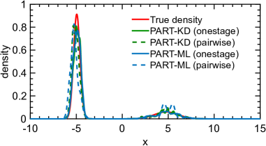
Figure 8: Bimodal posterior combined from 10 subsets. The results from PART-KD/PART-ML multiscale histograms are shown for (1) one-stage combination with local Gaussian smoothing (2) pairwise combination with local Gaussian smoothing.

Rare Bernoulli Example

The left panel of Figure 9 shows additional results of posteriors aggregated from PART-KD/PART-ML random tree ensemble with several alternative combination strategies, which complement the results presented in Figure 2 of the main text. All of the produced posteriors correctly locate the posterior mass despite the heterogeneity of subset posteriors. The fake “ripples” produced by pairwise ML aggregation are caused by local Gaussian smoothing.

Also, the right panel of Figure 9 shows that the posteriors produced by nonparametric and semiparametric methods miss the right scale.

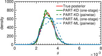
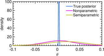
Figure 9: Posterior of the probability $\theta$ of a rare event combined from $M=15$ subsets of independent Bernoulli trials. Left: the results from KD/ML multiscale histograms are shown for (1) one-stage combination with local Gaussian smoothing (2) pairwise combination with local Gaussian smoothing. Right: posterior aggregated from nonparametric and semiparametric methods.

Appendix F: Supplement to Bayesian Logistic Regression

Figure 10 additionally plots the prediction accuracy against the length of subset chains supplied to the aggregation algorithms, for Bayesian logistic regression on two real datasets. For simplicity, the same number of posterior samples from all subset chains are aggregated, with the first 20% discarded as burn-in. As a reference, we also show the result for running the full chain. As can be seen from Figure 10, the performance of PART-KD/ML agrees with that of the full chain as the number of posterior samples increase, validating the theoretical results presented in Theorem 1 and Theorem 2 in the main text.

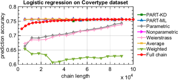
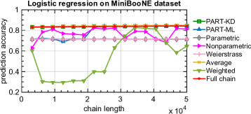
Figure 10: Prediction accuracy versus the length of subset chains on the covertype and the MiniBooNE dataset.

References

- [1] Max Welling and Yee W Teh. Bayesian learning via stochastic gradient langevin dynamics. In Proceedings of the 28th International Conference on Machine Learning (ICML-11), 2011.
- [2] Dougal Maclaurin and Ryan P Adams. Firefly Monte Carlo: Exact MCMC with subsets of data. Proceedings of the conference on Uncertainty in Artificial Intelligence (UAI), 2014.
- [3] Steven L Scott, Alexander W Blocker, Fernando V Bonassi, Hugh A Chipman, Edward I George, and Robert E McCulloch. Bayes and big data: The consensus Monte Carlo algorithm. In EFaBBayes 250 conference, volume 16, 2013.
- [4] Stanislav Minsker, Sanvesh Srivastava, Lizhen Lin, and David Dunson. Scalable and robust bayesian inference via the median posterior. In Proceedings of the 31st International Conference on Machine Learning (ICML-14), 2014.
- [5] Sanvesh Srivastava, Volkan Cevher, Quoc Tran-Dinh, and David B Dunson. WASP: Scalable Bayes via barycenters of subset posteriors. In Proceedings of the 18th International Conference on Artificial Intelligence and Statistics (AISTATS), volume 38, 2015.
- [6] Willie Neiswanger, Chong Wang, and Eric Xing. Asymptotically exact, embarrassingly parallel MCMC. arXiv preprint arXiv:1311.4780, 2013.
- [7] Xiangyu Wang and David B Dunson. Parallel MCMC via Weierstrass sampler. arXiv preprint arXiv:1312.4605, 2013.
- [8] Linxi Liu and Wing Hung Wong. Multivariate density estimation based on adaptive partitioning: Convergence rate, variable selection and spatial adaptation. arXiv preprint arXiv:1401.2597, 2014.
- [9] Manuel Blum, Robert W Floyd, Vaughan Pratt, Ronald L Rivest, and Robert E Tarjan. Time bounds for selection. Journal of Computer and System Sciences, 7(4):448–461, 1973.
- [10] Jon Louis Bentley. Multidimensional binary search trees used for associative searching. Communications of the ACM, 18(9):509–517, 1975.
- [11] Leo Breiman. Random forests. Machine Learning, 45(1):5–32, 2001.
- [12] Leo Breiman. Bagging predictors. Machine Learning, 24(2):123–140, 1996.
- [13] Xiaotong Shen and Wing Hung Wong. Convergence rate of sieve estimates. The Annals of Statistics, pages 580–615, 1994.
- [14] Nils Lid Hjort and Ingrid K Glad. Nonparametric density estimation with a parametric start. The Annals of Statistics, pages 882–904, 1995.
- [15] Heikki Haario, Marko Laine, Antonietta Mira, and Eero Saksman. DRAM: efficient adaptive MCMC. Statistics and Computing, 16(4):339–354, 2006.
- [16] Heikki Haario, Eero Saksman, and Johanna Tamminen. An adaptive Metropolis algorithm. Bernoulli, pages 223–242, 2001.
- [17] Jock A Blackard and Denis J Dean. Comparative accuracies of neural networks and discriminant analysis in predicting forest cover types from cartographic variables. In Proc. Second Southern Forestry GIS Conf, pages 189–199, 1998.
- [18] Byron P Roe, Hai-Jun Yang, Ji Zhu, Yong Liu, Ion Stancu, and Gordon McGregor. Boosted decision trees as an alternative to artificial neural networks for particle identification. Nuclear Instruments and Methods in Physics Research Section A: Accelerators, Spectrometers, Detectors and Associated Equipment, 543(2):577–584, 2005.
- [19] M. Lichman. UCI machine learning repository, 2013.
- [20] Robert Tibshirani. Regression shrinkage and selection via the lasso. Journal of the Royal Statistical Society. Series B (Methodological), pages 267–288, 1996.

References

- [1] Max Welling and Yee W Teh. Bayesian learning via stochastic gradient langevin dynamics. In Proceedings of the 28th International Conference on Machine Learning (ICML-11), 2011.
- [2] Dougal Maclaurin and Ryan P Adams. Firefly Monte Carlo: Exact MCMC with subsets of data. Proceedings of the conference on Uncertainty in Artificial Intelligence (UAI), 2014.
- [3] Steven L Scott, Alexander W Blocker, Fernando V Bonassi, Hugh A Chipman, Edward I George, and Robert E McCulloch. Bayes and big data: The consensus Monte Carlo algorithm. In EFaBBayes 250 conference, volume 16, 2013.
- [4] Stanislav Minsker, Sanvesh Srivastava, Lizhen Lin, and David Dunson. Scalable and robust bayesian inference via the median posterior. In Proceedings of the 31st International Conference on Machine Learning (ICML-14), 2014.
- [5] Sanvesh Srivastava, Volkan Cevher, Quoc Tran-Dinh, and David B Dunson. WASP: Scalable Bayes via barycenters of subset posteriors. In Proceedings of the 18th International Conference on Artificial Intelligence and Statistics (AISTATS), volume 38, 2015.
- [6] Willie Neiswanger, Chong Wang, and Eric Xing. Asymptotically exact, embarrassingly parallel MCMC. arXiv preprint arXiv:1311.4780, 2013.
- [7] Xiangyu Wang and David B Dunson. Parallel MCMC via Weierstrass sampler. arXiv preprint arXiv:1312.4605, 2013.
- [8] Linxi Liu and Wing Hung Wong. Multivariate density estimation based on adaptive partitioning: Convergence rate, variable selection and spatial adaptation. arXiv preprint arXiv:1401.2597, 2014.
- [9] Manuel Blum, Robert W Floyd, Vaughan Pratt, Ronald L Rivest, and Robert E Tarjan. Time bounds for selection. Journal of Computer and System Sciences, 7(4):448–461, 1973.
- [10] Jon Louis Bentley. Multidimensional binary search trees used for associative searching. Communications of the ACM, 18(9):509–517, 1975.
- [11] Leo Breiman. Random forests. Machine Learning, 45(1):5–32, 2001.
- [12] Leo Breiman. Bagging predictors. Machine Learning, 24(2):123–140, 1996.
- [13] Xiaotong Shen and Wing Hung Wong. Convergence rate of sieve estimates. The Annals of Statistics, pages 580–615, 1994.
- [14] Nils Lid Hjort and Ingrid K Glad. Nonparametric density estimation with a parametric start. The Annals of Statistics, pages 882–904, 1995.
- [15] Heikki Haario, Marko Laine, Antonietta Mira, and Eero Saksman. DRAM: efficient adaptive MCMC. Statistics and Computing, 16(4):339–354, 2006.
- [16] Heikki Haario, Eero Saksman, and Johanna Tamminen. An adaptive Metropolis algorithm. Bernoulli, pages 223–242, 2001.
- [17] Jock A Blackard and Denis J Dean. Comparative accuracies of neural networks and discriminant analysis in predicting forest cover types from cartographic variables. In Proc. Second Southern Forestry GIS Conf, pages 189–199, 1998.
- [18] Byron P Roe, Hai-Jun Yang, Ji Zhu, Yong Liu, Ion Stancu, and Gordon McGregor. Boosted decision trees as an alternative to artificial neural networks for particle identification. Nuclear Instruments and Methods in Physics Research Section A: Accelerators, Spectrometers, Detectors and Associated Equipment, 543(2):577–584, 2005.
- [19] M. Lichman. UCI machine learning repository, 2013.
- [20] Robert Tibshirani. Regression shrinkage and selection via the lasso. Journal of the Royal Statistical Society. Series B (Methodological), pages 267–288, 1996.