Permutation Search Methods are Efficient,
Yet Faster Search is Possible

Abstract

We survey permutation-based methods for approximate $k$-nearest neighbor search. In these methods, every data point is represented by a ranked list of pivots sorted by the distance to this point. Such ranked lists are called permutations. The underpinning assumption is that, for both metric and non-metric spaces, the distance between permutations is a good proxy for the distance between original points. Thus, it should be possible to efficiently retrieve most true nearest neighbors by examining only a tiny subset of data points whose permutations are similar to the permutation of a query. We further test this assumption by carrying out an extensive experimental evaluation where permutation methods are pitted against state-of-the art benchmarks (the multi-probe LSH, the VP-tree, and proximity-graph based retrieval) on a variety of realistically large data set from the image and textual domain. The focus is on the high-accuracy retrieval methods for generic spaces. Additionally, we assume that both data and indices are stored in main memory. We find permutation methods to be reasonably efficient and describe a setup where these methods are most useful. To ease reproducibility, we make our software and data sets publicly available.

1 Introduction

Nearest-neighbor searching is a fundamental operation employed in many applied areas including pattern recognition, computer vision, multimedia retrieval, computational biology, and statistical machine learning. To automate the search task, real-world objects are represented in a compact numerical, e.g., vectorial, form and a distance function $d(x,y)$, e.g., the Euclidean metric $L_{2}$, is used to evaluate the similarity of data points $x$ and $y$. Traditionally, it assumed that the distance function is a non-negative function that is small for similar objects and large for dissimilar one. It is equal to zero for identical $x$ and $y$ and is always positive when objects are different.

This mathematical formulation allows us to define the nearest-neighbor search as a conceptually simple optimization procedure. Specifically, given a query data point $q$, the goal is to identify the nearest (neighbor) data point $x$, i.e., the point with the minimum distance value $d(x,q)$ among all data points (ties can be resolved arbitrarily). A natural generalization is a $k$-NN search, where we aim to find $k$ closest points instead of merely one. If the distance is not symmetric, two types of queries are considered: left and right queries. In a left query, a data point compared to the query is always the first (i.e., the left) argument of $d(x,y)$.

Despite being conceptually simple, finding nearest neighbors in efficient and effective fashion is a notoriously hard task, which has been a recurrent topic in the database community (see e.g. [45, 20, 2, 30]). The most studied instance of the problem is an exact nearest-neighbor search in vector spaces, where a distance function is an actual metric distance (a non-negative, symmetric function satisfying the triangle inequality). If the search is exact, we must guarantee that an algorithm always finds a true nearest-neighbor no matter how much computational resources such a quest may require. Comprehensive reviews of exact approaches for metric and/or vector spaces can be found in books by Zezula et al. [47] and Samet [37].

Yet, exact methods work well only in low dimensional metric spaces. Experiments showed that exact methods can rarely outperform the sequential scan when dimensionality exceeds ten [45]. This a well-known phenomenon known as “the curse of dimensionality”.

Furthermore, a lot of applications are increasingly relying on non-metric spaces (for a list of references related to computer vision see, e.g., a work by Jacobs et al. [26]). This is primarily because many problems are inherently non-metric [26]. Thus, using, a non-metric distance permits sometimes a better representation for a domain of interest. Unfortunately, exact methods for metric-spaces are not directly applicable to non-metric domains.

Compared to metric spaces, it is more difficult to design exact methods for arbitrary non-metric spaces, in particular, because they lack sufficiently generic yet simple properties such as the triangle inequality. When exact search methods for non-metric spaces do exist, they also seem to suffer from the curse of dimensionality [10, 9].

Approximate search methods are less affected by the curse of dimensionality [33] and can be used in various non-metric spaces when exact retrieval is not necessary [40, 23, 13, 10, 9]. Approximate search methods can be much more efficient than exact ones, but this comes at the expense of a reduced search accuracy. The quality of approximate searching is often measured using recall, which is equal to the average fraction of true neighbors returned by a search method. For example, if the method routinely misses every other true neighbor, the respective recall value is 50%.

Permutation-based algorithms is an important class of approximate retrieval methods that was independently introduced by Amato [3] and Chávez et al. [24]. It is based on the idea that if we rank a set of reference points–called pivots–with respect to distances from a given point, the pivot rankings produced by two near points should be similar. A number of methods based on this idea were recently proposed and evaluated [3, 24, 19, 11, 2] (these methods are briefly surveyed in § 2). However, a comprehensive evaluation that involves a diverse set of large metric and non-metric data sets (i.e., asymmetric and/or hard-to-compute distances) is lacking. In § 3, we fill this gap by carrying out an extensive experimental evaluation where these methods (implemented by us) are compared against some of the most efficient state-of-the art benchmarks. The focus is on the high-accuracy retrieval methods (recall close to 0.9) for generic spaces. Because distributed high-throughput main memory databases are gaining popularity (see., e.g. [28]), we focus on the case where data and indices are stored in main memory. Potentially, the data set can be huge, yet, we run experiments only with a smaller subset that fits into a memory of one server.

2 Permutation Methods

2.1 Core Principles

Permutation methods are filter-and-refine methods belonging to the class of pivoting searching techniques. Pivots (henceforth denoted as $\pi_{i}$) are reference points randomly selected during indexing. To create an index, we compute the distance from every data point $x$ to every pivot $\pi_{i}$. We then memorize either the original distances or some distance statistics in the hope that these statistics can be useful during searching. At search time, we compute distances from the query to pivots and prune data points using, e.g., the triangle inequality [37, 47] or its generalization for non-metric spaces [21].

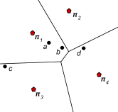
Figure 1: Voronoi diagram produced by four pivots $\pi_{i}$. The data points are $a$, $b$, $c$, and $d$. The distance is $L_{2}$.

Alternatively, rather than relying on distance values directly, we can use precomputed statistics to produce estimates for distances between the query and data points. In particular, in the case of permutation methods, we assess similarity of objects based on their relative distances to pivots. To this end, for each data point $x$, we arrange pivots $\pi_{i}$ in the order of increasing distances from $x$. The ties can be resolved, e.g., by selecting a pivot with the smallest index. Such a permutation (i.e., ranking) of pivots is essentially a vector whose $i$-th element keeps an ordinal position of the $i$-th pivot in the set of pivots sorted by their distances from $x$. We say that point $x$ induces the permutation.

Consider the Voronoi diagram in Figure 1 produced by pivots $\pi_{1}$, $\pi_{2}$, $\pi_{3}$, and $\pi_{4}$. Each pivot $\pi_{i}$ is associated with its own cell containing points that are closer to $\pi_{i}$ than to any other pivot $\pi_{j},i\neq j$. The neighboring cells of two pivots are separated by a segment of the line equidistant to these pivots. Each of the data points $a$, $b$, $c$, and $d$ “sits” in the cell of its closest pivot.

For the data point $a$, points $\pi_{1}$, $\pi_{2}$, $\pi_{3}$, and $\pi_{4}$ are respectively the first, the second, the third, and the forth closest pivots. Therefore, the point $a$ induces the permutation $(1,2,3,4)$. For the data point $b$, which is the nearest neighbor of $a$, two closest pivots are also $\pi_{1}$ and $\pi_{2}$. However, $\pi_{4}$ is closer than $\pi_{3}$. Therefore, the permutation induced by $b$ is $(1,2,4,3)$. Likewise, the permutations induced by $c$ and $d$ are $(2,3,1,4)$ and $(3,2,4,1)$, respectively.

The underpinning assumption of permutation methods is that most nearest neighbors can be found by retrieving a small fraction of data points whose pivot rankings, i.e., the induced permutations, are similar to the pivot ranking of the query. Two most popular choices to compare the rankings $x$ and $y$ are: Spearman’s rho distance (equal to the squared $L_{2}$) and the Footrule distance (equal to $L_{1}$) [14, 24]. More formally, $\mbox{SpearmanRho}(x,y)=\sum_{i}(x_{i}-y_{i})^{2}$ and $\mbox{Footrule}(x,y)=\sum_{i}|x_{i}-y_{i}|$. According to Chávez et al. [24] Spearman’s rho is more effective than the Footrule distance. This was also confirmed by our own experiments.

Converting the vector of distances to pivots into a permutation entails information loss, but this loss is not necessarily detrimental. In particular, our preliminary experiments showed that using permutations instead of vectors of original distances results in slightly better retrieval performance. The information about relative positions of the pivots can be further coarsened by binarization: All elements smaller than a threshold $b$ become zeros and elements at least as large as $b$ become ones [41]. The similarity of binarized permutations is computed via the Hamming distance.

In the example of Figure 1, the values of the Footrule distance between the permutation of $a$ and permutations of $b$, $c$, and $d$ are equal to 2, 4, and 6, respectively. Note that the Footrule distance on permutations correctly “predicts” the closest neighbor of $a$. Yet, the ordering of points based on the Footrule distance is not perfect: the Footrule distance from the permutation of $a$ to the permutation of its second nearest neighbor $d$ is larger than the Footrule distance to the permutation of the third nearest neighbor $c$.

Given the threshold $b=3$, the binarized permutations induced by $a$, $b$, $c$, and $d$ are equal to $(0,0,1,1)$, $(0,0,1,1)$, $(0,1,0,1)$, and $(1,0,1,0)$, respectively. In this example, the binarized permutation of $a$ and its nearest neighbor $b$ are equal, i.e., the distance between respective permutations is zero. When we compare $a$ to $c$ and $d$, the Hamming distance does not discriminate between $c$ and $d$ as their binary permutations are both at distance two from the binary permutation of $a$.

Permutation-based searching belongs to a class of filter-and-refine methods, where objects are mapped to data points in a low-dimensional space (usually $L_{1}$ or $L_{2}$). Given a permutation of a query, we carry out a nearest neighbor search in the space of permutations. Retrieved entries represent a (hopefully) small list of candidate data points that are compared directly to the query using the distance in the original space. The permutation methods differ in ways of producing candidate records, i.e., in the way of carrying out the filtering step. In the next sections we describe these methods in detail.

Permutation methods are similar to the rank-aggregation method OMEDRANK due to Fagin et al. [20]. In OMEDRANK there is a small set of voting pivots, each of which ranks data points based on a somewhat imperfect notion of the distance from points to the query (e.g., computed via a random projection). While each individual ranking is imperfect, a more accurate ranking can be achieved by rank aggregation. Thus, unlike permutation methods, OMEDRANK uses pivots to rank data points and aims to find an unknown permutation of data points that reconciles differences in data point rankings in the best possible way. When such a consolidating ranking is found, the most highly ranked objects from this aggregate ranking can be used as answers to a nearest-neighbor query. Finding the aggregate ranking is an NP-complete problem that Fagin et al. [20] solve only heuristically. In contrast, permutation methods use data points to rank pivots and solve a much simpler problem of finding already known and computed permutations of pivots that are the best matches for the query permutation.

Table 1: Summary of Data Sets

Name	Distance	# of rec.	Brute-force	In-memory	Dimens.	Source
	function		search (sec)	size
Metric Data
CoPhIR	$L_{2}$	$5\cdot 10^{6}$	0.6	5.4GB	282	MPEG7 descriptors [7]
SIFT	$L_{2}$	$5\cdot 10^{6}$	0.3	2.4GB	128	SIFT descriptors [27]
ImageNet	SQFD[4]	$1\cdot 10^{6}$	4.1	0.6 GB	N/A	Signatures generated from
						ImageNet LSVRC-2014 [36]
Non-Metric Data
Wiki-sparse	Cosine sim.	$4\cdot 10^{6}$	1.9	3.8GB	$10^{5}$	Wikipedia TF-IDF vectors
						generated via Gensim [35]
Wiki-8	KL-div/JS-div	$2\cdot 10^{6}$	0.045/0.28	0.13GB	8	LDA (8 topics) generated
						from Wikipedia via Gensim [35]
Wiki-128	KL-div/JS-div	$2\cdot 10^{6}$	0.22/4	2.1GB	128	LDA (128 topics) generated
						from Wikipedia via Gensim [35]
DNA	Normalized	$1\cdot 10^{6}$	3.5	0.03GB	N/A	Sampled from the Human Genome
	Levenshtein					with sequence length $\mathcal{N}(32,4)$

2.2 Brute-force Searching of Permutations

In this approach, the filtering stage is implemented as a brute-force comparison of the query permutation against the permutations of the data with subsequent selection of the $\gamma$ entries that are $\gamma$-nearest objects in the space of permutations. A number of candidate entries $\gamma$ is a parameter of the search algorithm that is often understood as a fraction (or percentage) of the total number of points. Because the distance in the space of permutations is not a perfect proxy for the original distance, to answer a $k$-NN-query with high accuracy, the number of candidate records has to be much larger than $k$ (see § 3.4).

A straightforward implementation of brute-force searching relies on a priority queue. Chávez et al. [24] proposed to use incremental sorting as a more efficient alternative. In our experiments with the $L_{2}$ distance, the latter approach is twice as fast as the approach relying on a standard C++ implementation of a priority queue.

The cost of the filtering stage can be reduced by using binarized permutations [41]. Binarized permutations can be stored compactly as bit arrays. Computing the Hamming distance between bit arrays can be done efficiently by XOR-ing corresponding computer words and counting the number of non-zero bits of the result. For bit-counting, one can use a special instruction available on many modern CPUs.

The brute-force searching in the permutation space, unfortunately, is not very efficient, especially if the distance can be easily computed: If the distance is “cheap” (e.g., $L_{2}$) and the index is stored in main memory, the brute-force search in the space of permutations is not much faster than the brute-force search in the original space.

2.3 Indexing of Permutations

To reduce the cost of the filtering stage of permutation-based searching, three types of indices were proposed: the Permutation Prefix Index (PP-Index) [19], existing methods for metric spaces [22], and the Metric Inverted File (MI-file) [3].

Permutations are integer vectors whose values are between one and the total number of pivots $m$. We can view these vectors as sequences of symbols over a finite alphabet and index these sequences using a prefix tree. This approach is implemented in the PP-index. At query time, the method aims to retrieve $\gamma$ candidates by finding permutations that share a prefix of a given length with the permutation of the query object. This operation can be carried out efficiently via the prefix tree constructed at index time. If the search generates fewer candidates than a specified threshold $\gamma$, the procedure is recursively repeated using a shorter prefix. For example, the permutations of points $a$, $b$, $c$, and $d$ in Figure 1 can be seen as strings 1234, 1243, 2314, and 3241. The permutation of points $a$ and $b$, which are nearest neighbors, share a two-character prefix with $a$. In contrast, permutations of points $c$ and $d$, which are more distant from $a$ than $b$, have no common prefix with $a$.

To achieve good recall, it may be necessary to use short prefixes. However, longer prefixes are more selective than shorter ones (i.e., they generate fewer candidate records) and are, therefore, preferred for efficiency reasons. In practice, a good trade-off between recall and efficiency is typically achieved only by building several copies of the PP-index (using different subsets of pivots) [2].

Figueroa and Fredriksson experimented with indexing permutations using well-known data structures for metric spaces [22]. Indeed, the most commonly used permutation distance: Spearman’s rho, is a monotonic transformation (squaring) of the Euclidean distance. Thus, it should be possible to find $\gamma$ nearest neighbors by indexing permutations, e.g., in a VP-tree [46, 43].

Amato and Savino proposed to index permutation using an inverted file [3]. They called their method the MI-file. To build the MI-file, they first select $m$ pivots and compute their permutations/rankings induced by data points. For each data point, $m_{i}\leq m$ most closest pivots are indexed in the inverted file. Each posting is a pair $(pos(\pi_{i},x),x)$, where $x$ is the identifier of the data point and $pos(\pi_{i},x)$ is a position of the pivot in the permutation induced by $x$. Postings of the same pivot are sorted by pivot’s positions.

Consider the example of Figure 1 and imagine that we index two most closest pivots (i.e., $m_{i}=2$). The point $a$ induces the permutation $(1,2,3,4)$. Two closest pivots $\pi_{1}$ and $\pi_{2}$ generate postings $(1,a)$ and $(2,a)$. The point $b$ induces the permutation $(1,2,4,3)$. Again, $\pi_{1}$ and $\pi_{2}$ are two pivots closest to $b$. The respective postings are $(1,b)$ and $(2,b)$. The permutation of $c$ is $(2,3,1,4)$. Two closest pivots are $\pi_{1}$ and $\pi_{3}$. The respective postings are $(2,c)$ and $(1,c)$. The permutation of $d$ is $(3,2,4,1)$. Two closest pivots are $\pi_{2}$ and $\pi_{4}$ with corresponding postings $(2,d)$ and $(1,d)$.

At query time, we select $m_{s}\leq m_{i}$ pivots closest to the query $q$ and retrieve respective posting lists. If $m_{s}=m_{i}=m$, it is possible to compute the exact Footrule distance (or Spearman’s rho) between the query permutation and the permutation induced by data points. One possible search algorithm keeps an accumulator (initially set to zero) for every data point. Posting lists are read one by one: For every encountered posting $(pos(\pi_{i},x),x)$ we increase the accumulator of $x$ by the value $|pos(\pi_{i},x)-pos(\pi_{i},q)|$. If the goal is to compute Spearman’s rho, the accumulator is increased by $|pos(\pi_{i},x)-pos(\pi_{i},q)|^{2}$.

If $m_{s}<m$, by construction of the posting lists, using the inverted index, it is possible to obtain rankings of only $m_{s}<m$ pivots. For the remaining, $m-m_{s}$ pivots we pessimistically assume that their rankings are all equal to $m$ (the maximum possible value). Unlike the case $m_{i}=m_{s}=m$, all accumulators are initially set to $m_{s}\cdot m$. Whenever we encounter a posting posting $(pos(\pi_{i},x),x)$ we subtract $m-|pos(\pi_{i},x)-pos(\pi_{i},q)|$ from the accumulator of $x$.

Consider again the example of Figure 1. Let $m_{i}=m_{s}=2$ and $a$ be the query point. Initially, the accumulators of $b$, $c$, and $d$ contain values $4\cdot 2=8$. Because $m_{s}=2$, we read posting lists only of the two closest pivots for the query point $a$, i.e., $\pi_{1}$ and $\pi_{2}$. The posting lists of $\pi_{1}$ is comprised of $(1,a)$, $(1,b)$, and $(2,c)$. On reading them (and ignoring postings related to the query $a$), accumulators $b$ and $c$ are decreased by $4-|1-1|=4$ and $4-|1-2|=3$, respectively. The posting lists of $\pi_{2}$ are $(2,a)$, $(2,b)$, and $(2,d)$. On reading them, we subtract $4-|2-2|=4$ from each of the accumulators $b$ and $d$. In the end, the accumulators $b$, $c$, $d$ are equal to 0, 5, and 4. Unlike the case when we compute the Footrule distance between complete permutation, the Footrule distance on truncated permutations correctly predicts the order of three nearest neighbors of $a$.

Using fewer pivots at retrieval time allows us to reduce the number of processed posting lists. Another optimization consists in keeping posting lists sorted by pivots position $pos(\pi_{i},x)$ and retrieving only the entries satisfying the following restriction on the maximum position difference: $|pos(\pi_{i},x)-pos(\pi_{i},q)|\leq D$, where $D$ is a method parameter. Because posting list entries are sorted by pivot positions, the first and the last entry satisfying the maximum position difference requirement can be efficiently found via the binary search.

Tellez et al. [42] proposed a modification of the MI-file which they called a Neighborhood APProximation index (NAPP). In the case of NAPP, there also exist a large set of $m$ pivots of which only $m_{i}<m$ pivots (most closest to inducing data points) are indexed. Unlike the MI-file, however, posting lists contain only object identifiers, but no positions of pivots in permutations. Thus, it is not possible to compute an estimate for the Footrule distance by reading only posting lists. Therefore, instead of an estimate for the Footrule distance, the number of most closest common pivots is used to sort candidate objects. In addition, the candidate objects sharing with the query fewer than $t$ closest pivots are discarded ($t$ is a parameter). For example, points $a$ and $b$ in Figure 1 share the same common pivot $\pi_{1}$. At the same time $a$ does not share any closest pivot with points $d$ and $c$. Therefore, if we use $a$ as a query, the point $b$ will be considered to be the best candidate point.

Chávez et al. [25] proposed a single framework that unifies several approaches including PP-index, MI-file, and NAPP. Similar to the PP-index, permutations are viewed as strings over a finite alphabet. However, these strings are indexed using a special sequence index (rather than a prefix tree) that efficiently supports rank and select operations. These operations can be used to simulate various index traversal modes, including, e.g., retrieval of all strings whose $i$-th symbol is equal to a given one.

3 Experiments

3.1 Data Sets and Distance Functions

We employ three image data sets: CoPhIR, SIFT, ImageNet, and several data sets created from textual data. The smallest data set (DNA) has one million entries, while the largest one (CoPhIR) contains five million high-dimensional vectors. All data sets derived from Wikipedia were generated using the topic modelling library GENSIM [35]. The data set meta data is summarized in Table 1. Below, we describe our data sets in detail.

CoPhIR is a five million subset of MPEG7 descriptors downloaded from the website of the Institute of the National Research Council of Italy[7].

SIFT is a five million subset of SIFT descriptors (from the learning subset) downloaded from a TEXMEX collection website[27].

In experiments involving CoPhIR and SIFT, we employed $L_{2}$ to compare unmodified, i.e., raw visual descriptors. We implemented an optimized procedure to compute $L_{2}$ that relies on Single Instruction Multiple Data (SIMD) operations available on Intel-compatible CPUs. Using this implementation, it is possible to carry out about 30 million $L_{2}$ computations per second using SIFT vectors or 10 million $L_{2}$ computations using CoPhIR vectors.

ImageNet collection comprises one million signatures extracted from LSVRC-2014 data set [36], which contains 1.2 million high resolution images. We implemented our own code to extract signatures following the method of Beecks [4]. For each image, we selected $10^{4}$ pixels randomly and mapped them into 7-dimensional feature space: three color, two position, and two texture dimensions.

The features were clustered by the standard $k$-means algorithm with 20 clusters. Then, each cluster was represented by an 8-dimensional vector, which included a 7-dimensional centroid and a cluster weight (the number of cluster points divided by $10^{4}$).

Table 2: Index Size and Creation Time for Various Data Sets

	VP-tree		NAPP		LSH		Brute-force filt.		$k$-NN graph
Metric Data
CoPhIR	5.4 GB	(0.5min)	6 GB	(6.8min)	13.5 GB	(23.4min)			7 GB	(52.1min)
SIFT	2.4 GB	(0.4min)	3.1 GB	(5min)	10.6 GB	(18.4min)			4.4 GB	(52.2min)
ImageNet	1.2 GB	(4.4min)	0.91 GB	(33min)			12.2 GB	(32.3min)	1.1 GB	(127.6min)
Non-Metric Data
Wiki-sparse			4.4 GB	(7.9min)					5.9 GB	(231.2min)
Wiki-8 (KL-div)	0.35 GB	(0.1min)	0.67 GB	(1.7min)					962 MB	(11.3min)
Wiki-128 (KL-div)	2.1 GB	(0.2min)	2.5 GB	(3.1min)					2.9 GB	(14.3min)
Wiki-8 (JS-div)	0.35 GB	(0.1min)	0.67 GB	(3.6min)					2.4 GB	(89min)
Wiki-128 (JS-div)	2.1 GB	(1.2min)	2.5 GB	(36.6min)					2.8 GB	(36.1min)
DNA	0.13 GB	(0.9min)	0.32 GB	(15.9min)			61 MB	(15.6min)	1.1 GB	(88min)
Note: The indexing algorithms of NAPP and $k$-NN graphs used four threads.
In all but two cases (DNA and Wiki-8 with JS-divergence), we build the $k$-NN graph using the Small World algorithm [31].
In the case of DNA or Wiki-8 with JS-divergence, we build the $k$-NN graph using the NN-descent algorithm [16].

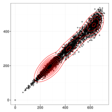
(a) SIFT ($L_{2}$) rnd-proj

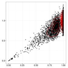
(b) Wiki-sparse (cos.) rnd-proj

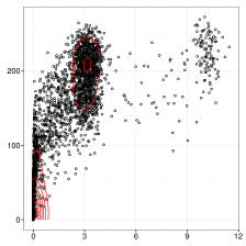
(c) Wiki-8 (KL-div) perm

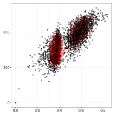
(d) DNA (norm. Leven.) perm

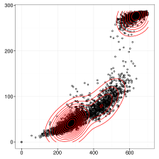
(e) SIFT ($L_{2}$) perm

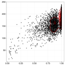
(f) Wiki-sparse perm

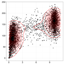
(g) Wiki-128 (KL-div) perm

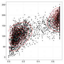
(h) Wiki-128 (JS-div) perm

Figure 2: Distance values in the projected space (on the y-axis) plotted against original distance values (on the x-axis). Plots 2a and 2b use random projections. The remaining plots rely on permutations. Dimensionality of the target space is 64. All plots except Plot 2b represent projections to $L_{2}$. In Plot 2b the target distance function is the cosine similarity. Distances are computed for pairs of points sampled at random. Sampling is conducted from two strata: a complete subset and a set of points that are 100 nearest neighbors of randomly selected points. All data sets have one million entries.

Images were compared using a metric function called the Signature Quadratic Form Distance (SQFD). This distance is computed as a quadratic form, where the matrix is re-computed for each pair of images using a heuristic similarity function applied to cluster representatives. It is a distance metric defined over vectors from an infinite-dimensional space such that each vector has only finite number of non-zero elements. For further details, please, see the thesis of Beecks [4]. SQFD was shown to be effective [4]. Yet, it is nearly two orders of magnitude slower compared to $L_{2}$.

Wiki-sparse is a set of four million sparse TF-IDF vectors (created via GENSIM [35]). On average, these vectors have 150 non-zero elements out of $10^{5}$. Here we use a cosine similarity, which is a symmetric non-metric distance:

$$d(x,y)=1-\left(\sum_{i=1}^{n}x_{i}y_{i}\right)\left(\sum_{i=1}^{n}x_{i}^{2}\right)^{-1/2}\left(\sum_{i=1}^{n}y_{i}^{2}\right)^{-1/2}.$$

Computation of the cosine similarity between sparse vectors relies on an efficient procedure to obtain an intersection of non-zero element indices. To this end, we use an all-against-all SIMD comparison instruction as was suggested by Schlegel et al. [38]. This distance function is relatively fast being only about 5x slower compared to $L_{2}$.

Wiki-$i$ consist of dense vectors of topic histograms created using the Latent Dirichlet Allocation (LDA)[6]. The index $i\in\{8,128\}$ denotes the number of topics. To create these sets, we trained a model on one half of the Wikipedia collection and then applied it to the other half (again using GENSIM [35]). Zero values were replaced by small numbers ($10^{-5}$) to avoid division by zero in the distance calculations. Two distance functions were used for these data sets: the Kullback-Leibler (KL) divergence: $\sum_{i=1}^{n}x_{i}\log\frac{x_{i}}{y_{i}}$ and its symmetrized version called the Jensen-Shannon (JS) divergence:

$$d(x,y)=\frac{1}{2}\sum_{i=1}^{n}\left[x_{i}\log x_{i}+y_{i}\log y_{i}-(x_{i}+y_{i})\log\frac{x_{i}+y_{i}}{2}\right].$$

Both the KL- and the JS-divergence are non-metric distances. Note that the KL-divergence is not even symmetric.

Our implementation of the KL-divergence relies on the precomputation of logarithms at index time. Therefore, during retrieval it is as fast as $L_{2}$. In the case of JS-divergence, it is not possible to precompute $\log(x_{i}+y_{i})$ and, thus, it is about 10-20 times slower compared to $L_{2}$.

DNA is a collection of DNA sequences sampled from the Human Genome . Starting locations were selected randomly and uniformly (however, lines containing the symbol N were excluded). The length of the sequence was sampled from $\mathcal{N}(32,4)$. The employed distance function was the normalized Levenshtein distance. This non-metric distance is equal to the minimum number of edit operations (insertions, deletions, substitutions), needed to convert one sequence into another, divided by the maximum of the sequence lengths.

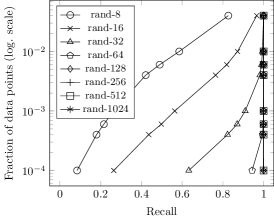
(a) SIFT ($L_{2}$)

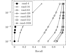
(b) Wiki-sparse (cosine similarity)

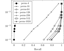
(c) Wiki-8 (KL-divergence)

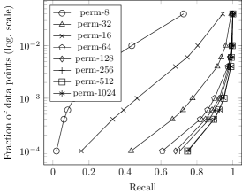
(d) SIFT ($L_{2}$)

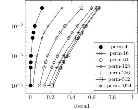
(e) Wiki-sparse (cosine similarity)

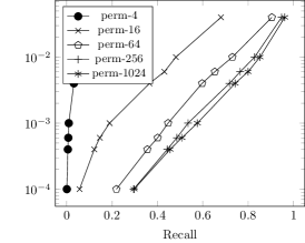
(f) Wiki-128 (KL-divergence)

(g) DNA (Normalized Levenshtein)

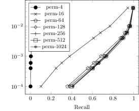
(h) ImageNet (SQFD)

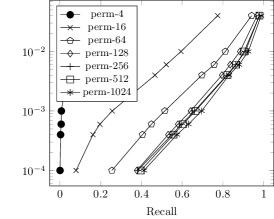
(i) Wiki-128 (JS-divergence)

Figure 3: A fraction of candidate records that are necessary to retrieve to ensure a desired recall level (10-NN search). The candidate entries are ranked in a projected space using either the cosine similarity (only for Wiki-sparse) or $L_{2}$ (for all the other data sets). Two types of projections are used: random projections (rand) and permutations (perm). In each plot, there are several lines that represent projections of different dimensionality. Each data (sub)set in this experiment contains one million entries.

3.2 Tested Methods

Table 2 lists all implemented methods and provides information on index creation time and size.

Multiprobe-LSH (MPLSH) is implemented in the library LSHKit . It is designed to work only for $L_{2}$. Some parameters are selected automatically using the cost model proposed by Dong et al. [17]. However, the size of the hash table $H$, the number of hash tables $L$, and the number of probes $T$ need to be chosen manually. We previously found that (1) $L=50$ and $T=10$ provided a near optimal performance and (2) performance is not affected much by small changes in $L$ and $T$ [9]. This time, we re-confirmed this observation by running a small-scale grid search in the vicinity of $L=50$ and $T=50$ for $H$ equal to the number of points plus one. The MPLSH generates a list of candidates that are directly compared against the query. This comparison involves the optimized SIMD implementation of $L_{2}$.

VP-tree is a classic space decomposition tree that recursively divides the space with respect to a randomly chosen pivot $\pi$[46, 43]. For each partition, we compute a median value $R$ of the distance from $\pi$ to every other point in the current partition. The pivot-centered ball with the radius $R$ is used to partition the space: the inner points are placed into the left subtree, while the outer points are placed into the right subtree (points that are exactly at distance $R$ from $\pi$ can be placed arbitrarily).

Partitioning stops when the number of points falls below the threshold $b$. The remaining points are organized in a form of a bucket. In our implementation, all points in a bucket are stored in the same chunk of memory. For cheap distances (e.g., $L_{2}$ and KL-div) this placing strategy can halve retrieval time.

If the distance is the metric, the triangle inequality can be used to prune unpromising partitions as follows: imagine that $r$ is a radius of the query and the query point is inside the pivot-centered ball (i.e., in the left subtree). If $R-d(\pi,q)>r$, the right partition cannot have an answer, i.e., the right subtree can be safely pruned. If the query point is in the right partition, we can prune the left subtree if $d(\pi,q)-R>r$. The nearest-neighbor search is simulated as a range search with a decreasing radius: Each time we evaluate the distance between $q$ and a data point, we compare this distance with $r$. If the distance is smaller, it becomes a new value of $r$. In the course of traversal, we first visit the closest subspace (e.g., the left subtree if the query is inside the pivot-centered ball).

For a generic, i.e., not necessarily metric, space, the pruning conditions can be modified. For example, previously we used a liner “stretching” of the triangle inequality [9]. In this work, we employed a simple polynomial pruner. More specifically, the right partition can be pruned if the query is in the left partition and $(R-d(\pi,q))^{\beta}\alpha_{left}>r$. The left partition can be pruned if the query is in the right partition and $(d(\pi,q)-R)^{\beta}\alpha_{right}>r$.

We used $\beta=2$ for the KL-divergence and $\beta=1$ for every other distance function. The optimal parameters $\alpha_{left}$ and $\alpha_{right}$ can be found by a trivial grid-search-like procedure with a shrinking grid step [9] (using a subset of data).

$k$-NN graph (a proximity graph) is a data structure in which data points are associated with graph nodes and $k$ edges are connected to $k$ nearest neighbors of the node. The search algorithm relies on a concept “the closest neighbor of my closest neighbor is my neighbor as well.” This algorithm can start at an arbitrary node and recursively transition to a neighbor point (by following the graph edge) that is closest to the query. This greedy algorithm stops when the current point $x$ is closer to the query than any of the $x$’s neighbors. However, this algorithm can be trapped in a local minima [15]. Alternatively, the termination condition can be defined in terms of an extended neighborhood [39, 31].

Constructing an exact $k$-NN graph is hardly feasible for a large data set, because, in the worst case, the number of distance computations is $O(n^{2})$, where $n$ in the number of data points. While there are amenable metric spaces where an exact graph can be computed more efficiently than in $O(n^{2})$, see e.g. [32], the quadratic cost appear to be unavoidable in many cases, especially if the distance is not a metric or the intrinsic dimensionality is high.

An approximate $k$-NN graph can be constructed more efficiently. In this work, we employed two different graph construction algorithms: the NN-descent proposed by Dong et al. [16] and the search-based insertion algorithm used by Malkov et al. [31]. The NN-descent is an iterative procedure initialized with randomly selected nearest neighbors. In each iteration, a random sample of queries is selected to participate in neighborhood propagation.

Malkov et al. [31] called their method a Small World (SW) graph. The graph-building algorithm finds an insertion point by running the same algorithm that is used during retrieval. Multiple insertion attempts are carried out starting from a random point.

The open-source implementation of NN-descent is publicly available online.. However, it comes without a search algorithm. Thus, we used the algorithm due to Malkov et al. [31], which was available in the Non-Metric Space Library [8]. We applied both graph construction algorithms. Somewhat surprisingly, in all but two cases, NN-descent took (much) longer time to converge. For each data set, we used the graph-construction algorithm that performed better on a subset of the data. Both graph construction algorithms are computationally expensive and are, therefore, constructed in a multi-threaded mode (four threads). Tuning of $k$-NN graphs involved manual selection of two parameters $k$ and the decay coefficient (tuning was carried out on a subset of data). The latter parameter, which is used only for NN-descent, defines the convergence speed.

Brute-force filtering is a simple approach where we exhaustively compare the permutation of the query against permutation of every data point. We then use incremental sorting to select $\gamma$ permutations closest to the query permutation. These $\gamma$ entries represent candidate records compared directly against the query using the original distance.

As noted in § 2, the cost of the filtering stage is high. Thus, we use this algorithm only for the computationally intensive distances: SQFD and the Normalized Levenshtein distance. Originally, both in the case of SQFD and Normalized Levenshtein distance, good performance was achieved with permutations of the size 128. However, Levenshtein distance was applied to DNA sequences, which were strings whose average length was only 32. Therefore, using uncompressed permutations of the size 128 was not space efficient (128 32-bit integers use 512 bytes). Fortunately, we can achieve the same performance using bit-packed binary permutations with 256 elements, each of which requires only 32 bytes.

The optimal permutation size was found by a small-scale grid search (again using a subset of data). Several values of $\gamma$ (understood as a fraction of the total number of points) were manually selected to achieve recall in the range 0.85-0.9.

NAPP is a neighborhood approximation index described in § 2 [42]. Our implementation is different from the proposition of Chávez et al. [25] and Tellez et al. [41] in at least two ways: (1) we do not compress the index and (2) we use a simpler algorithm, namely, the ScanCount, to merge posting lists [29]. For each entry in the database, there is a counter. When we read a posting list entry corresponding to the object $i$, we increment counter $i$. To improve cache utilization and overall performance, we split the inverted index into small chunks, which are processed one after another. Before each search counters are zeroed using the function memset from a standard C library.

Tuning NAPP involves selection of three parameters $m$ (the total number of pivots), $m_{i}$ (the number of indexed pivots), and $t$. The latter is equal to the minimum number of indexed pivots that has to be shared between the query and a data point. By carrying out a small-scale grid search, we found that increasing $m$ improves both recall and decreases retrieval time, yet, improvement is small beyond $m=500$. At the same time, computation of one permutation entails computation of $m$ distances to pivots. Thus, larger values of $m$ incur higher indexing cost. Values of $m$ between 500 and 2000 provide a good trade-off. Because the indexing algorithm is computationally expensive, it is executed in a multi-threaded mode (four threads).

Increasing $m_{i}$ improves recall at the expense of retrieval efficiency: The larger is $m_{i}$, the more posting lists are to be processed at query time. We found that good results are achieved for $m_{i}=32$. Smaller values of $t$ result in high recall values. At the same time, they also produce a larger number of candidate records, which negatively affects performance. Thus, for cheap distances, e.g. $L_{2}$, we manually select the smallest $t$ that allows one to achieve a desired recall (using a subset of data). For more expensive distances, we have an additional filtering step (as proposed by Tellez et al. [41]), which involves sorting by the number of commonly indexed pivots.

Our initial assessment showed that NAPP was more efficient than the PP-index and at least as efficient MI-file, which agrees with results of Chávez et al. [11]. We also compared our NAPP implementation to that of Chávez et al. [11] using the same $L_{1}$ data set: $10^{6}$ normalized CoPhIR descriptors. At 95% recall, Chávez et al. [11] achieve a 14x speed up, while we achieve a 15x speed up (relative to respective brute-force search implementations). Thus, our NAPP implementation is a competitive benchmark. Additionally we benchmark our own implementation of Fagin et al.’s OMEDRANK algorithm [20] and found NAPP to be more efficient. We also experimented with indexing permutations using the VP-tree, yet, this algorithm was either outperformed by the VP-tree in the original space or by NAPP.

3.3 Experimental Setup

Experiments were carried out on an Linux Intel Xeon server (3.60 GHz, 32GB memory) in a single threaded mode using the Non-Metric Space Library [8] as an evaluation toolkit. The code was written in C++ and compiled using GNU C++ 4.8 with the -Ofast optimization flag. Additionally, we used the flag -march=native to enable SIMD extensions.

We evaluated performance of a 10-NN search using a procedure similar to a five-fold cross validation. We carried out five iterations, in which a data set was randomly split into two parts. The larger part was indexed and the smaller part comprised queries . For each split, we evaluated retrieval performance by measuring the average retrieval time, the improvement in efficiency (compared to a single-thread brute-force search), the recall, the index creation time, and the memory consumption. The retrieval time, recall, and the improvement in efficiency were aggregated over five splits. To simplify our presentation, in the case of non-symmetric KL-divergence, we report results only the for the left queries. Results for the right queries are similar.

Because we are interested in high-accuracy (near 0.9 recall) methods, we tried to tune parameters of the methods (using a subset of the data) so that their recall falls in the range 0.85-0.95. Method-specific tuning procedures are described in respective subsections of Section 3.2.

3.4 Quality of Permutation-Based Projections

Recall that permutation methods are filter-and-refine approaches that map data from the original space to $L_{2}$ or $L_{1}$. Their accuracy depends on the quality of this mapping, which we assess in this subsection. To this end, we explore (1) the relationship between the original distance values and corresponding values in the projected space, (2) the relationship between the recall and the fraction of candidate records scanned in response to a query.

Figure 2 shows distance values in the original space (on the x-axis) vs. values in the projected space (on the y-axis) for eight combinations of data sets and distance functions. Points were randomly sampled from two strata: a complete subset and a set of points that are 100 nearest neighbors of randomly selected points. Of the presented panels, 2a and 2b correspond to the classic random projections. The remaining panels show permutation-based projections.

Classic random projections are known to preserve inner products and distance values [5]. Indeed, the relationship between the distance in the original and the projected space appears to be approximately linear in panels 2a and 2b. Therefore, it preserves the relative distance-based order of points with respect to a query. For example, there is a high likelihood for the nearest neighbor in the original space to remain the nearest neighbor in the projected space. In principle, any monotonic relationship—not necessarily linear–will suffice [40]. If the monotonic relationship holds at least approximately, the projection typically distinguishes between points close to the query and points that are far away.

For example, the projection in panel 2e appears to be quite good, which is not entirely surprising, because the original space is Euclidean. The projections in panels 2h and 2d are also reasonable, but not as good as one in panel 2e. The quality of projections in panels 2f and 2c is somewhat uncertain. The projection in panel 2g–which represents the non-symmetric and non-metric distance–is obviously poor. Specifically, there are two clusters: one is close to the query (in the original distance) and the other is far away. However, in the projected space these clusters largely overlap.

Figure 3 contains nine panels that plot recall (on x-axis) against a fraction of candidate records necessary to retrieve to ensure this recall level (on y-axis). In each plot, there are several lines that represent projections of different dimensionality. Good projections (e.g., random projections in panels 3a and 3b) correspond to steep curves: recall approaches one even for a small fraction of candidate records retrieved. Steepness depends on the projection dimensionality. However, good projection curves are steep even in relatively low dimensions.

The worst projection according to Figure 2 is in panel 2g. It corresponds to the Wiki-128 data set with distance measured by KL-divergence. Panel 3f in Figure 3, corresponding to this combination of the distance and the data set, also confirms the low quality of the projection. For example, given a permutation of dimensionality 1024, scanning 1% of the candidate permutations achieves roughly a 0.9 recall. An even worse projection example is in panel 3e. In this case, regardless of the dimensionality, scanning 1% of the candidate permutations achieves recall below 0.6.

At the same time, for majority of projections in other panels, scanning 1% of the candidate permutations of dimensionality 1024 achieves an almost perfect recall. In other words, for some data sets, it is, indeed, possible to obtain a small set of candidate entries containing a true near-neighbor by searching in the permutation space.

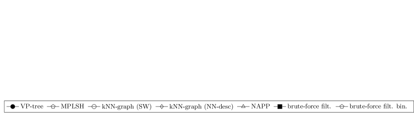
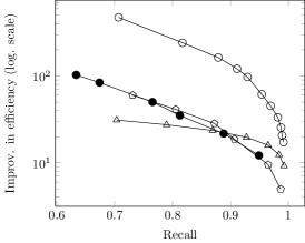
(a) SIFT ($L_{2}$)

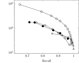
(b) CoPhIR ($L_{2}$)

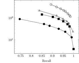
(c) ImageNet (SQFD)

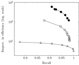
(d) Wiki-8 (KL-div.)

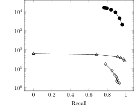
(e) Wiki-8 (JS-div.)

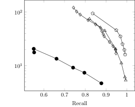
(f) DNA (Normalized Levenshtein)

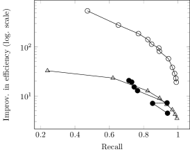
(g) Wiki-128 (KL-div.)

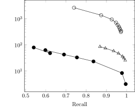
(h) Wiki-128 (JS-div.)

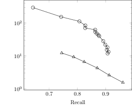
(i) Wiki-sparse (cosine simil.)

Figure 4: Improvement in efficiency vs. recall for various data sets (10-NN search). Each plot includes one of the two implemented $k$-NN graph algorithms: Small World (SW) or NN-descent (NN-desc).

3.5 Evaluation of Efficiency vs Recall

In this section, we use complete data sets listed in Table 1. Figure 4 shows nine data set specific panels with improvement in efficiency vs. recall. Each curve captures method-specific results with parameter settings tuned to achieve recall in the range of 0.85-0.95.

It can be seen that in most data sets the permutation method NAPP is a competitive baseline. In particular, panels 4a and 4b show NAPP outperforming the state-of-the art implementation of the multi-probe LSH (MPLSH) for recall larger than 0.95. This is consistent with findings of Chávez et al. [11].

In that, in our experiments, there was no single best method. $k$-NN graphs substantially outperform other methods in 6 out of 9 data sets. However, in low-dimensional data sets shown in panels 4d and 4e, the VP-tree outperforms the other methods by a wide margin. The Wiki-sparse data set (see panel 4i), which has high representational dimensionality, is quite challenging. Among implemented methods, only $k$-NN graphs are efficient for this set.

Interestingly, the winner in panel 4f is a brute-force filtering using binarized permutations. Furthermore, the brute-force filtering is also quite competitive in panel 4c, where it is nearly as efficient as NAPP. In both cases, the distance function is computationally intensive and a more sophisticated permutation index does not offer a substantial advantage over a simple brute-force search in the permutation space.

Good performance of $k$-NN graphs comes at the expense of long indexing time. For example, it takes almost four hours to built the index for the Wiki-sparse data set using as many as four threads (see Table 2). In contrast, it takes only 8 minutes in the case of NAPP (also using four threads). In general, the indexing algorithm of $k$-NN graphs is substantially slower than the indexing algorithm of NAPP: it takes up to an order of magnitude longer to build a $k$-NN graph. One exception is the case of Wiki-128 where the distance is the JS-divergence. For both NAPP and $k$-NN graph, the indexing time is nearly 40 minutes. However, the $k$-NN graph retrieval is an order of magnitude more efficient.

Both NAPP and the brute-force searching of permutations have high indexing costs compared to the VP-tree. This cost is apparently dominated by time necessary to compute permutations. Recall that obtaining a permutation entails $m$ distance computations. Thus, building an index entails $N\cdot m$ distance computations, where $N$ is the number of data points. In contrast, building the VP-tree requires roughly $N\cdot\log_{2}N/b$ distance computations, where $b$ is the size of the bucket. In our setup, $m>100$ while $\log_{2}N/b<20$. Therefore, the indexing step of permutation methods is typically much longer than that of the VP-tree.

Even though permutation methods may not be the best solutions when both data and the index are kept in main memory, they can be appealing in the case of disk-resident data [2] or data kept in a relational database. Indeed, as noted by Fagin et al. [20], indexes based on the inverted files are database friendly, because they require neither complex data structures nor many random accesses. Furthermore, deletion and addition of records can be easily implemented. In that, it is rather challenging to implement a dynamic version of the VP-tree on top of a relational database.

We also found that all evaluated methods perform reasonably well in the surveyed non-metric spaces. This might indicate that there is some truth to the two folklore wisdoms: (1) “the closest neighbor of my closest neighbor is my neighbor as well”, (2) “if one point is close to a pivot, but another is far away, such points cannot be close neighbors”. Yet, these wisdoms are not universal. For example, they are violated in one dimensional space with the “distance” $e^{-|x-y|}|x-y|$. In this space, points 0 and 1 are distant. However, we can select a large positive number that can be arbitrarily close to both of them, which results in violation of properties (1) and (2).

It seems that such a paradox does not manifest in the surveyed non-metric spaces. In the case of continuous functions, there is non-negative strictly monotonic transformation $f(x)\geq 0$, $f(0)=0$ such that $f(d(x,y))$ is a $\mu$-defective distance function. Thus, the distance satisfies the following inequality:

$$|f(d(q,a))-f(d(q,b))|\leq\mu f(d(a,b)),\mu>0$$ (1)

Indeed, a monotonic transformation of the cosine similarity is the metric function (i.e, the angular distance) [44]. The square root of the JS-divergence is metric function called Jensen-Shannon distance [18]. The square root of all Bregman divergences (which include the KL-divergence) is $\mu$-defective as well [1]. The normalized Levenshtein distance is a non-metric distance. However, for many realistic data sets, the triangle inequality is rarely violated. In particular, we verified that this is the case of our data set. The normalized Levenshtein distance is approximately metric and, thus, it is approximately $\mu$-defective (with $\mu=1$).

If Inequality (1) holds, due to properties of $f(x)$, $d(a,b)=0$ and $d(q,a)=0$ implies $d(q,b)=0$. Similarly if $d(q,b)=0$, but $d(q,a)\neq 0$, $d(a,b)$ cannot be zero either. Moreover, for a sufficiently large $d(q,a)$ and small $d(q,b)$, $d(a,b)$ cannot be small. Thus, the two folklore wisdoms are true if the strictly monotonic distance transformation is $\mu$-defective.

4 Conclusions

We benchmarked permutation methods for approximate $k$-nearest neighbor search for generic spaces where both data and indices are stored in main memory (aiming for high-accuracy retrieval). We found these filter-and-refine methods to be reasonably efficient. The best performance is achieved either by NAPP or by brute-force filtering of permutations. For example, NAPP can outperform the multi-probe LSH in $L_{2}$. However, permutation methods can be outstripped by either VP-trees or $k$-NN graphs, partly because the filtering stage can be costly.

We believe that permutation methods are most useful in non-metric spaces of moderate dimensionality when: (1) The distance function is expensive (or the data resides on disk); (2) The indexing costs of $k$-NN graphs are unacceptably high; (3) There is a need for a simple, but reasonably efficient, implementation that operates on top of a relational database.

5 Acknowledgments

This work was partially supported by the iAd Center  and the Open Advancement of Question Answering Systems (OAQA) group .

We also gratefully acknowledge help of several people. In particular, we are thankful to Anna Belova for helping edit the experimental and concluding sections. We thank Christian Beecks for answering questions regarding the Signature Quadratic Form Distance (SQFD) [4]; Daniel Lemire for providing the implementation of the SIMD intersection algorithm; Giuseppe Amato and Eric S. Tellez for help with data sets; Lu Jiang for the helpful discussion of image retrieval algorithms and for providing useful references.

We thank Nikita Avrelin and Alexander Ponomarenko for porting their proximity-graph based retrieval algorithm to the Non-Metric Space Library. The results of the preliminary evaluation were published elsewhere [34]. In the current publication, we use improved versions of the NAPP and baseline methods. In particular, we improved the tunning algorithm of the VP-tree and we added another implementation of the proximity-graph based retrieval [16]. Furthermore, we experimented with a more diverse collection of (mostly larger) data sets. In particular, because of this, we found that proximity-based retrieval may not be an optimal solution in all cases, e.g., when the distance function is expensive to compute.

References

- [1] A. Abdullah, J. Moeller, and S. Venkatasubramanian. Approximate bregman near neighbors in sublinear time: Beyond the triangle inequality. In Proceedings of the twenty-eighth annual symposium on Computational geometry, pages 31–40. ACM, 2012.
- [2] G. Amato, C. Gennaro, and P. Savino. MI-file: using inverted files for scalable approximate similarity search. Multimedia tools and applications, 71(3):1333–1362, 2014.
- [3] G. Amato and P. Savino. Approximate similarity search in metric spaces using inverted files. In Proceedings of the 3rd international conference on Scalable information systems, InfoScale ’08, pages 28:1–28:10, ICST, Brussels, Belgium, Belgium, 2008. ICST (Institute for Computer Sciences, Social-Informatics and Telecommunications Engineering).
- [4] C. Beecks. Distance based similarity models for content based multimedia retrieval. PhD thesis, 2013.
- [5] E. Bingham and H. Mannila. Random projection in dimensionality reduction: applications to image and text data. In Proceedings of the seventh ACM SIGKDD international conference on Knowledge discovery and data mining, pages 245–250. ACM, 2001.
- [6] D. M. Blei, A. Y. Ng, and M. I. Jordan. Latent dirichlet allocation. the Journal of machine Learning research, 3:993–1022, 2003.
- [7] P. Bolettieri, A. Esuli, F. Falchi, C. Lucchese, R. Perego, T. Piccioli, and F. Rabitti. CoPhIR: a test collection for content-based image retrieval. CoRR, abs/0905.4627v2, 2009.
- [8] L. Boytsov and B. Naidan. Engineering efficient and effective non-metric space library. In SISAP, pages 280–293, 2013. Available at https://github.com/searchivarius/nmslib
- [9] L. Boytsov and B. Naidan. Learning to prune in metric and non-metric spaces. In NIPS, pages 1574–1582, 2013.
- [10] L. Cayton. Fast nearest neighbor retrieval for bregman divergences. In ICML, pages 112–119, 2008.
- [11] E. Chávez, M. Graff, G. Navarro, and E. Téllez. Near neighbor searching with k nearest references. Information Systems, 2015.
- [12] E. Chávez, G. Navarro, R. Baeza-Yates, and J. L. Marroquín. Searching in metric spaces. ACM computing surveys (CSUR), 33(3):273–321, 2001.
- [13] L. Chen and X. Lian. Efficient similarity search in nonmetric spaces with local constant embedding. Knowledge and Data Engineering, IEEE Transactions on, 20(3):321–336, 2008.
- [14] P. Diaconis. Group representations in probability and statistics. Lecture Notes-Monograph Series, pages i–192, 1988.
- [15] W. Dong. High-Dimensional Similarity Search for Large Datasets. PhD thesis, Princeton University, 2011.
- [16] W. Dong, C. Moses, and K. Li. Efficient k-nearest neighbor graph construction for generic similarity measures. In Proceedings of the 20th international conference on World wide web, pages 577–586. ACM, 2011.
- [17] W. Dong, Z. Wang, W. Josephson, M. Charikar, and K. Li. Modeling lsh for performance tuning. In Proceedings of the 17th ACM conference on Information and knowledge management, CIKM ’08, pages 669–678, New York, NY, USA, 2008. ACM.
- [18] D. M. Endres and J. E. Schindelin. A new metric for probability distributions. Information Theory, IEEE Transactions on, 49(7):1858–1860, 2003.
- [19] A. Esuli. PP-index: Using permutation prefixes for efficient and scalable approximate similarity search. Proceedings of LSDS-IR, 2009, 2009.
- [20] R. Fagin, R. Kumar, and D. Sivakumar. Efficient similarity search and classification via rank aggregation. In Proceedings of the 2003 ACM SIGMOD International Conference on Management of Data, SIGMOD ’03, pages 301–312, New York, NY, USA, 2003. ACM.
- [21] A. Faragó, T. Linder, and G. Lugosi. Fast nearest-neighbor search in dissimilarity spaces. Pattern Analysis and Machine Intelligence, IEEE Transactions on, 15(9):957–962, 1993.
- [22] K. Figueroa and K. Frediksson. Speeding up permutation based indexing with indexing. In Proceedings of the 2009 Second International Workshop on Similarity Search and Applications, pages 107–114. IEEE Computer Society, 2009.
- [23] K.-S. Goh, B. Li, and E. Chang. Dyndex: a dynamic and non-metric space indexer. In Proceedings of the tenth ACM international conference on Multimedia, pages 466–475. ACM, 2002.
- [24] E. C. Gonzalez, K. Figueroa, and G. Navarro. Effective proximity retrieval by ordering permutations. Pattern Analysis and Machine Intelligence, IEEE Transactions on, 30(9):1647–1658, 2008.
- [25] Edgar Chávez, Mario Graff, Gonzalo Navarro, and Eric Sadit Téllez. Near neighbor searching with K nearest references. Inf. Syst., 51:43–61, 2015.
- [26] D. Jacobs, D. Weinshall, and Y. Gdalyahu. Classification with nonmetric distances: Image retrieval and class representation. Pattern Analysis and Machine Intelligence, IEEE Transactions on, 22(6):583–600, 2000.
- [27] H. Jégou, R. Tavenard, M. Douze, and L. Amsaleg. Searching in one billion vectors: re-rank with source coding. In Acoustics, Speech and Signal Processing (ICASSP), 2011 IEEE International Conference on, pages 861–864. IEEE, 2011.
- [28] R. Kallman, H. Kimura, J. Natkins, A. Pavlo, A. Rasin, S. Zdonik, E. P. C. Jones, S. Madden, M. Stonebraker, Y. Zhang, J. Hugg, and D. J. Abadi. H-store: A high-performance, distributed main memory transaction processing system. Proc. VLDB Endow., 1(2):1496–1499, Aug. 2008.
- [29] C. Li, J. Lu, and Y. Lu. Efficient merging and filtering algorithms for approximate string searches. In Data Engineering, 2008. ICDE 2008. IEEE 24th International Conference on, pages 257–266. IEEE, 2008.
- [30] Y. Liu, J. Cui, Z. Huang, H. Li, and H. T. Shen. Sk-lsh: An efficient index structure for approximate nearest neighbor search. Proc. VLDB Endow., 7(9):745–756, May 2014.
- [31] Y. Malkov, A. Ponomarenko, A. Logvinov, and V. Krylov. Approximate nearest neighbor algorithm based on navigable small world graphs. Information Systems, 45:61–68, 2014.
- [32] R. Paredes, E. Chávez, K. Figueroa, and G. Navarro. Practical construction of k-nearest neighbor graphs in metric spaces. In Experimental Algorithms, pages 85–97. Springer, 2006.
- [33] V. Pestov. Indexability, concentration, and {VC} theory. Journal of Discrete Algorithms, 13(0):2 – 18, 2012. Best Papers from the 3rd International Conference on Similarity Search and Applications (SISAP 2010).
- [34] A. Ponomarenko, N. Avrelin, B. Naidan, and L. Boytsov. Comparative analysis of data structures for approximate nearest neighbor search. In DATA ANALYTICS 2014, The Third International Conference on Data Analytics, pages 125–130, 2014.
- [35] R. Řehůřek and P. Sojka. Software Framework for Topic Modelling with Large Corpora. In Proceedings of the LREC 2010 Workshop on New Challenges for NLP Frameworks, pages 45–50, Valletta, Malta, May 2010. ELRA.
- [36] O. Russakovsky, J. Deng, H. Su, J. Krause, S. Satheesh, S. Ma, Z. Huang, A. Karpathy, A. Khosla, M. Bernstein, A. C. Berg, and L. Fei-Fei. ImageNet Large Scale Visual Recognition Challenge, 2014.
- [37] H. Samet. Foundations of Multidimensional and Metric Data Structures. Morgan Kaufmann Publishers Inc., 2005.
- [38] B. Schlegel, T. Willhalm, and W. Lehner. Fast sorted-set intersection using simd instructions. In ADMS@ VLDB, pages 1–8, 2011.
- [39] T. B. Sebastian and B. B. Kimia. Metric-based shape retrieval in large databases. In Pattern Recognition, 2002. Proceedings. 16th International Conference on, volume 3, pages 291–296. IEEE, 2002.
- [40] T. Skopal. Unified framework for fast exact and approximate search in dissimilarity spaces. ACM Trans. Database Syst., 32(4), Nov. 2007.
- [41] E. S. Téllez, E. Chávez, and A. Camarena-Ibarrola. A brief index for proximity searching. In Progress in Pattern Recognition, Image Analysis, Computer Vision, and Applications, pages 529–536. Springer, 2009.
- [42] E. S. Tellez, E. Chávez, and G. Navarro. Succinct nearest neighbor search. Information Systems, 38(7):1019–1030, 2013.
- [43] J. K. Uhlmann. Satisfying general proximity/similarity queries with metric trees. Information processing letters, 40(4):175–179, 1991.
- [44] S. Van Dongen and A. J. Enright. Metric distances derived from cosine similarity and pearson and spearman correlations. arXiv preprint arXiv:1208.3145, 2012.
- [45] R. Weber, H. J. Schek, and S. Blott. A quantitative analysis and performance study for similarity-search methods in high-dimensional spaces. In Proceedings of the 24th International Conference on Very Large Data Bases, pages 194–205. Morgan Kaufmann, August 1998.
- [46] P. N. Yianilos. Data structures and algorithms for nearest neighbor search in general metric spaces. In SODA, volume 93, pages 311–321, 1993.
- [47] P. Zezula, G. Amato, V. Dohnal, and M. Batko. Similarity Search: The Metric Space Approach (Advances in Database Systems). Springer-Verlag New York, Inc., Secaucus, NJ, USA, 2005.