Quantum interference effects in laser spectroscopy of
muonic hydrogen, deuterium, and helium-3

Abstract

Quantum interference between energetically close states is theoretically investigated, with the state structure being observed via laser spectroscopy. In this work, we focus on hyperfine states of selected hydrogenic muonic isotopes, and on how quantum interference affects the measured Lamb shift. The process of photon excitation and subsequent photon decay is implemented within the framework of nonrelativistic second-order perturbation theory. Due to its experimental interest, calculations are performed for muonic hydrogen, deuterium, and helium-3. We restrict our analysis to the case of photon scattering by incident linear polarized photons and the polarization of the scattered photons not being observed. We conclude that while quantum interference effects can be safely neglected in muonic hydrogen and helium-3, in the case of muonic deuterium there are resonances with close proximity, where quantum interference effects can induce shifts up to a few percent of the linewidth, assuming a pointlike detector. However, by taking into account the geometry of the setup used by the CREMA collaboration, this effect is reduced to less than 0.2% of the linewidth in all possible cases, which makes it irrelevant at the present level of accuracy.

I Introduction

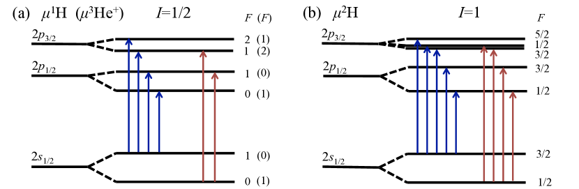
Figure 1: (Color online) $2s$ and $2p$ level structure (not in scale) for $\mu^{1}$H, $\mu^{3}$He⁺ (a) and $\mu^{2}$H (b). Allowed electric dipole transitions are also shown. $I$ and $F$ are the nuclear spin and total angular momentum, respectively.

Quantum interference (QI) corrections were introduced in the seminal work of Low Low (1952), where the quantum electrodynamics (QED) theory of the natural line profile in atomic physics was formulated. These corrections go beyond the resonant approximation and set a limit for which a standard Lorentzian line profile can be used to describe a resonance. Often referred to as nonresonant corrections Labzowsky et al. (1994, 2001, 2009), they contain the full quantum interference between the main resonant channel and other non-resonant channels, which leads to an asymmetry of the line profile. Therefore, the fitting of spectroscopy data with Lorentzian profiles becomes ambiguous, since it leads to energy shifts that depend on the measurement process itself Labzowsky et al. (1994, 2001, 2009); Brown et al. (2013). A careful analysis of the limits of the resonance approximation is thus mandatory for high-precision optical and microwave spectroscopy experiments.

The first calculation of QI was made for the Lamb shift in hydrogen-like (H-like) ions and for the photon scattering case Low (1952). It was found to be relatively small, of the order of $\delta_{\tiny\mbox{QI}}/\Gamma\approx\alpha(\alpha Z)^{2}$, compared to the linewidth $\Gamma$. Here $\delta_{\tiny\mbox{QI}}$ is the line shift due to QI, $\alpha$ is the fine structure constant and $Z$ is the atomic number. Thus, for some time, little interest has been addressed to these corrections in optical measurements of H-like ions. Since the late 1990s, high-precision measurements of the $1s-2s$ transition frequency in hydrogen renewed the interest in these corrections Huber et al. (1999); Niering et al. (2000); Parthey et al. (2011). Numerous theoretical calculations of QI were then made for H-like ions Labzowsky et al. (2001); Jentschura and Mohr (2002); Labzowsky et al. (2007, 2009) with astrophysical interest Karshenboim and Ivanov (2008) and application to laser-dressed atoms Jentschura et al. (2003). QI has also been studied in other atomic systems and processes during the last decades, mainly because near and crossed resonances of hyperfine states can enhance the QI effects Franken (1961); Walkup et al. (1982); Sansonetti et al. (2011). QI effects Horbatsch and Hessels (2010); Marsman et al. (2012, 2012, 2014) have been shown to be responsible for discrepant measurements of the helium fine structure Marsman et al. (2015, 2015) and the lithium charge radii determined by the isotope shift Brown et al. (2013). The lithium experiment Brown et al. (2013) gives a beautiful experimental demonstration of the geometry dependence of the QI effect. Very recently, QI effects in two-photon frequency-comb spectroscopy have been investigated, too Yost et al. (2014).

Table 1: Calculated energy differences of $\mu^{1}$H, $\mu^{2}$H and $\mu^{3}$He⁺ Borie (2012); Antognini et al. (2013) states relative to the lowest $n=2$ hyperfine state, which are $2s_{1/2}^{F=0}$, $2s_{1/2}^{F=1/2}$ and $2s_{1/2}^{F=1}$, respectively. $\Gamma_{2p}$ is the respective approximate linewidth.

		GHz	meV
$\mu^{1}$H	$2s_{1/2}(F=1)$	5520	22.83
	$2p_{1/2}(F=0)$	51631	213.53
	$2p_{1/2}(F=1)$	53521	221.35
	$2p_{3/2}(F=1)$	54616	225.88
	$2p_{3/2}(F=2)$	55402	229.12
	$\Gamma_{2p}$ Milotti (1998)	18.5	0.0765
$\mu^{2}$H	$2s_{1/2}(F=3/2)$	1485	6.143
	$2p_{1/2}(F=1/2)$	49680	205.46
	$2p_{1/2}(F=3/2)$	50182	207.54
	$2p_{3/2}(F=3/2)$	52016	215.12
	$2p_{3/2}(F=1/2)$	52104	215.49
	$2p_{3/2}(F=5/2)$	52286	216.24
	$\Gamma_{2p}$ Milotti (1998)	19.5	0.0806
$\mu^{3}$He	$2s_{1/2}(F=0)$	41443	171.40
	$2p_{1/2}(F=1)$	311456	1288.08
	$2p_{1/2}(F=0)$	325633	1346.71
	$2p_{3/2}(F=2)$	347860	1438.63
	$2p_{3/2}(F=1)$	353731	1462.92
	$\Gamma_{2p}$	318.7	0.1318

In this work, we calculate the QI shifts for $2s$$\rightarrow$$2p$ transitions in H-like muonic atoms with hyperfine structure. The physical process considered here is the photon scattering of initial $2s$ states to final $1s$ states, with an incident photon energy that is resonant with intermediate $2p$ states. Figure 1 recalls the $2s\rightarrow 2p$ level structures that are considered in this work. The level structures and linewidths Borie (2012); Milotti (1998) of the $2p$ states are given in Table 1. The theoretical formalism used here can be traced back to recent works Safari et al. (2012, 2015); Brown et al. (2013).

Hyperfine states in $\mu^{1}$H are separated by several hundred GHz Martynenko (2005, 2008); Borie (2005, 2012), and have linewidths of a few tens of GHz Milotti (1998). Thus, it is expected that QI plays a small role and cannot be responsible for the so-called “proton radius puzzle”, where a discrepancy of four linewidths was observed in the experiments of the Charge Radius Experiment with Muonic Atoms (CREMA) collaboration Pohl et al. (2010); Antognini et al. (2013). Nevertheless, these systematics need to be carefully evaluated and quantified, since they have contributions similar to small QED corrections (e.g. sixth-order contributions Borie (2012)) and thus may impact precise determinations of the proton charge radius. Since resonances in $\mu^{3}$He⁺ Antognini et al. (2011); Nebel et al. (2012) have been measured recently, values of the corresponding QI contributions are presented here, too. In the case of $\mu^{2}$H, there is a close energy proximity between the states $2p_{3/2}^{F=1/2}$ and $2p_{3/2}^{F=3/2}$ of $\approx 87$ GHz and hence, it is expected that QI effects could be much higher.

II Theory

Photon scattering is a two-step process consisting of photon excitation with subsequent photon decay, which is formally equivalent to Raman anti-Stokes scattering. It is described by second-order theories (e.g. Kramers-Heisenberg formula Loudon (2000), or S-matrix Akhiezer and Berestetskii (1965)), which overall converge to the following scattering amplitude (velocity gauge and atomic units) from initial to final states Akhiezer and Berestetskii (1965); Loudon (2000); Safari et al. (2012),

$$\displaystyle\mathcal{M}_{i\rightarrow f}^{{\bm{\varepsilon}_{1}}{\bm{\varepsilon}_{2}}}=\displaystyle{\displaystyle\sum_{\nu}}\left[\frac{\mathinner{\langle{f}|}\alpha{\bm{p}}\cdot{\bm{\varepsilon}_{2}}\mathinner{|{\nu}\rangle}\mathinner{\langle{\nu}|}\alpha{\bm{p}}\cdot{\bm{\varepsilon}_{1}}\mathinner{|{i}\rangle}}{\omega_{\nu i}-\omega_{1}-i\Gamma_{\nu}/2}\right.$$

$$\left.+\frac{\mathinner{\langle{f}|}\alpha{\bm{p}}\cdot{\bm{\varepsilon}_{1}}\mathinner{|{\nu}\rangle}\mathinner{\langle{\nu}|}\alpha{\bm{p}}\cdot{\bm{\varepsilon}_{2}}\mathinner{|{i}\rangle}}{\omega_{\nu i}+\omega_{2}-i\Gamma_{\nu}/2}\right],$$ (1)

where $\mathinner{|{i}\rangle}$, $\mathinner{|{\nu}\rangle}$, and $\mathinner{|{f}\rangle}$ represent the initial, intermediate and final hyperfine states of the muonic atom or ion. $\omega_{\nu i}=E_{\nu}-E_{i}$ is the transition frequency between $\mathinner{|{\nu}\rangle}$ and $\mathinner{|{i}\rangle}$. The dipole approximation, $\alpha{\bm{p}}\cdot{\bm{\varepsilon}_{\gamma}}$ ($\gamma=1,2$) is used, where, ${\bm{p}}$ is the linear momentum operator and ${\bm{\varepsilon}_{\gamma}}$ is the incident (scattered) photon polarization. The summation over the intermediate states $\mathinner{|{\nu}\rangle}$ runs over all solutions of the Dirac spectrum of the muonic atom (ion) with hyperfine structure. All states are considered with a well-defined total atomic angular momentum $F$, projection along the quantified axis $m$, and total orbiting particle angular momentum $J$ Safari et al. (2014); thus the contribution of off-diagonal terms (mixing between the $2p_{1/2}^{F=1}$ and $2p_{3/2}^{F=1}$ states) Pachucki (1996) is considered null. $\Gamma_{\nu}$ is the full width at half maximum for an isolated Lorentzian line of the excited state, where we assume $\Gamma_{2p_{j}^{F}}\equiv\Gamma_{2p}$.

The incident photon energies studied in this work comprise the near-resonant region of the $2s\rightarrow 2p$ transitions. This includes only the resonances illustrated in Fig. 1. Hence, we restrict the summation $\nu$ to the $2p$ states of the terms $\omega_{2s2p}-\omega_{1}$ [first part of the right side of Eq. (1)].

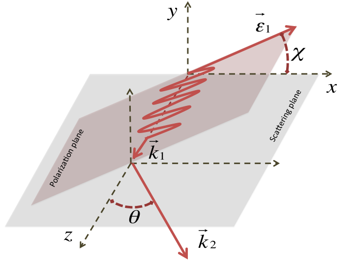
Figure 2: (Color online) Adopted geometry for photon scattering of incident linear polarized photons with momentum ${\bm{k}_{1}}$ and polarization ${\bm{\varepsilon}_{1}}$ and scattered photon momentum ${\bm{k}_{2}}$, uniquely defined by $\theta$. The scattered photon’s polarization is not observed in our measurements and is thus not illustrated.

Energy conservation leads to $E_{i}-E_{f}=\omega_{2}-\omega_{1}$ Safari et al. (2012) between the initial ($E_{i}$) and final ($E_{f}$) energy states and the energy of the incident ($\omega_{1}$) and scattered ($\omega_{2}$) photons; thus only one of the photon energies is independent. Using this relation, it is convenient to introduce the energy sharing parameter $u=\omega_{1}/\omega_{r}$ defined by the fraction of the incident photon energy relative to the lowest resonant energy $\omega_{r}$ of a given muonic atom with initial $F_{i}$ (see Fig. 1).

Motived by the experimental configuration, we consider incident photons having linear polarization and non-observation of scattered photon’s polarization, as illustrated in Fig. 2 . If we define the scattering plane, containing both photon momenta (${\bm{k}_{1}}$ and ${\bm{k}_{2}}$), then a single polar angle $\theta$ is sufficient for describing the angular distribution of ${\bm{k}_{2}}$.

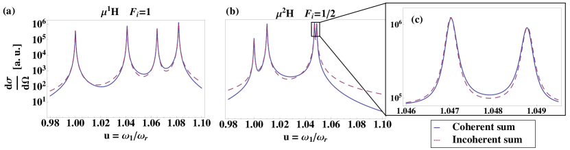
Figure 3: (Color online) Scattering differential cross-section (9) at $\theta=90$ °and $\chi=0$ °  for $\mu^{1}$H (a) and $\mu^{2}$H (b) versus photon frequency. A zoom plot of the two close-lying resonances for $\mu^{2}$H is given in the right panel (c). Solid blue lines correspond to the full evaluation of Eq. (9), while the dashed red curves account for only the first term in the right side of Eq. (9) (sum of Lorentzian profiles).

The corresponding differential cross section of the amplitude in Eq. (1) for all the mentioned approximations is given by Akhiezer and Berestetskii (1965)

$$\frac{d\sigma}{d\Omega}(u,\theta,\chi)=\frac{1}{(2F_{i}+1)}\sum_{\tiny\begin{array}[]{c}m_{i},F_{f},m_{f},J_{f}\\ \bm{\varepsilon_{2}}\end{array}}\left|\mathcal{M}_{i\rightarrow f}^{\bm{\varepsilon_{1}},\bm{\varepsilon_{2}}}\right|^{2}\approx\hskip 28.45274pt$$ (4)

$$\frac{\omega_{r}^{2}uu_{fi}^{3}}{(2F_{i}+1)}\sum_{\tiny\begin{array}[]{c}m_{i},F_{f},m_{f},J_{f}\\ \bm{\varepsilon_{2}}\end{array}}\left|\sum_{F_{\nu},m_{\nu},J_{\nu}}\frac{D_{F_{i}m_{i}J_{i}}^{F_{\nu}m_{\nu}J_{\nu}}\left(D_{F_{\nu}m_{\nu}J_{\nu}}^{F_{f}m_{f}J_{f}}\right)^{*}}{\mathrm{bar}{\omega}_{\nu i}-u-i\mathrm{bar}{\Gamma}_{\nu}/2}\right|^{2},\hskip 8.67787pt$$ (7)

(8)

where $\mathrm{bar}{\omega}_{\nu i}=\omega_{\nu i}/\omega_{r}$, $\mathrm{bar}{\Gamma}_{\nu}=\Gamma_{\nu}/\omega_{r}$ and $u_{fi}=u+\mathrm{bar}{\omega}_{fi}$. In Eq. (8), it is assumed that the initial state of the atom is unpolarized and that the level and magnetic sublevels of the final state, as well as the scattered photon’s polarization (${\bm{\varepsilon}_{2}}$) remains unobserved in the scattering process. $D_{F^{\prime}m^{\prime}J^{\prime}}^{FmJ}$ are the dipole matrix elements (length gauge). Equation (8) can be further rearranged as a sum of Lorentzian components $\Lambda_{J_{i}J_{\nu}}^{F_{i}F_{\nu}}(\theta,\chi)$, and cross terms $\Xi_{J_{i}J_{\nu}J_{\nu}^{\prime}}^{F_{i}F_{\nu}F_{\nu}^{\prime}}(\theta,\chi)$, similar to Ref. Brown et al. (2013). For our particular geometry and atomic system, the result is given by

$$\frac{d\sigma}{d\Omega}(u,\theta,\chi)=\frac{\omega_{r}^{2}uu_{fi}^{3}\mathcal{S}_{f\nu i}^{2}}{(2F_{i}+1)}\left(\sum_{\small F_{\nu},J_{\nu}}\frac{\Lambda_{J_{i}J_{\nu}}^{F_{i}F_{\nu}}(\theta,\chi)}{(\mathrm{bar}{\omega}_{\nu i}-u)^{2}+(\mathrm{bar}{\Gamma}_{\nu}/2)^{2}}+\sum_{(F^{\prime}_{\nu},J^{\prime}_{\nu})>(F_{\nu},J_{\nu})}\frac{\Xi_{J_{i}J_{\nu}J_{\nu}^{\prime}}^{F_{i}F_{\nu}F_{\nu}^{\prime}}(\theta,\chi)}{(\mathrm{bar}{\omega}_{\nu i}-u-i\mathrm{bar}{\Gamma}_{\nu}/2)(\mathrm{bar}{\omega}_{\nu^{\prime}i}-u+i\mathrm{bar}{\Gamma}_{\nu}/2)}\right)~{},$$ (9)

where the second summation over $F^{\prime}_{\nu}$ and $J^{\prime}_{\nu}$ runs for non-repeated values of $F_{\nu}$ and $J_{\nu}$ of the first summation. The quantities defined by

$$\Lambda_{J_{i}J_{\nu}}^{F_{i}F_{\nu}}(\theta,\chi)=\sum_{m_{i},F_{f},m_{f},J_{f},{\bm{\varepsilon}_{2}}}\left|\Omega_{J_{i}J_{\nu}J_{f}}^{F_{i}F_{\nu}F_{f}}(\theta,\chi,{\bm{\varepsilon}_{2}})\right|^{2}~{},\hskip 28.45274pt$$

and

$$\Xi_{J_{i}J_{\nu}J_{\nu}^{\prime}}^{F_{i}F_{\nu}F_{\nu}^{\prime}}(\theta,\chi)=\hskip 163.60333pt$$

$$2\mbox{Re}\left[\sum_{\tiny\begin{array}[]{c}m_{i},F_{f}\\ m_{f},J_{f},{\bm{\varepsilon}_{2}}\end{array}}\Omega_{J_{i}J_{\nu}J_{f}}^{F_{i}F_{\nu}F_{f}}(\theta,\chi,{\bm{\varepsilon}_{2}})\left(\Omega_{J_{i}J^{\prime}_{\nu}J_{f}}^{F_{i}F^{\prime}_{\nu}F_{f}}(\theta,\chi,{\bm{\varepsilon}_{2}})\right)^{*}\right]~{},$$ (12)

(13)

contain all the polarization and geometrical dependencies. $D_{F^{\prime}m^{\prime}J^{\prime}}^{FmJ}$, $\Omega_{J_{i}J_{\nu}J_{f}}^{F_{i}F_{\nu}F_{f}}(\theta,\chi,{\bm{\varepsilon}_{2}})$ and $\mathcal{S}_{f\nu i}$ are given in the Appendix.

The differential cross section of Eqs. (8) and (9) contains a coherent summation over resonant excitation channels; thus it takes into account channel-interference between neighboring resonances. However, as can be observed in Eq. (9), if cross terms $\Xi$ were removed, it reduces to an incoherent sum of independent Lorentzian profiles. The QI effects are thus included in those cross terms.

III Results and Discussion

In this section, we present and discuss results for the QI contribution in several muonic atoms taking into account Eqs. (9) and (13), first assuming a pointlike detector and later the CREMA geometry. The influence of the geometric and polarization conditions on the QI is well described in Ref. Brown et al. (2013) and is reproduced in the present work. We thus restrict our geometrical settings to the perpendicular observation ($\theta=90^{o}$) of scattered photons and to the case of horizontally and vertically polarized photons with respect to the scattering plane ($\chi=0^{o}$ and $\chi=90^{o}$). Figure 3 displays the scattering cross section for the $2s\rightarrow 2p\rightarrow 1s$ processes in $\mu^{1}$H and $\mu^{2}$H, on one hand, having the full coherent summation of Eq. (8) (i.e. with QI), on the other hand, having the summation restricted to only the Lorentzian terms [neglecting cross-terms in Eq. (9)]. The peaks correspond to the respective transitions shown in Fig. 1. As it is observed, the influence of QI is more noticeable in regions between resonances, where no dominant excitation channels exist. Close to resonances, the influence of QI is approximately equivalent to shifting the peak position, as shown in the zoom plot of Fig. 3.

We determine this shift in each resonance by generating a pseudo spectrum that follows the theoretical profile of Eq. (9) and fitting it with an incoherently sum of Lorentzians (as performed in the data analysis of the CREMA experiments). Fits are done using the ROOT/MINUIT package min . All fit parameters (position, amplitude, and linewidth) are free fit parameters for each transition. The fit range is chosen sufficiently large, such that the fit results do not depend on it. The shifts of the fitted resonance position, $\delta_{\tiny\mbox{QI}}$, normalized to $\Gamma_{2p}$, for each resonance and muonic atoms are given in Table 2. Overall, with the exception of some resonances in $\mu^{2}$H, QI produces relative shifts $\delta_{\tiny\mbox{QI}}$ less than 3% of $\Gamma_{2p}$. For $\mu^{1}$H and $\mu^{3}$He⁺, the shifts are of the order of $\sim 0.2\%-1.7$% ($\sim$36 MHz$-310$ MHz) and $\sim 0.2\%-3.2$% ($\sim 0.6$ GHz$-10$ GHz) of their linewidths, respectively.

Table 2: Shift of the line center due to QI contribution for $\mu^{1}$H, $\mu^{3}$He⁺ and $\mu^{2}$H. $\mathinner{|{i}\rangle}$ and $\mathinner{|{\nu}\rangle}$ stand for the initial and resonant atomic state, respectively. Values of $\delta$ divided by $\Gamma_{2p}$ are given for a pointlike detector with vertical ($\delta_{\tiny\mbox{QI}}^{\perp}$,  $\chi=90$ °, $\theta=90$ °) and horizontal ($\delta_{\tiny\mbox{QI}}^{\parallel}$, $\chi=0$ °, $\theta=90$ °) polarization cases, as well as for the CREMA setup geometry ($\delta_{\tiny\mbox{QI}}^{*}$).

	$\mathinner{|{i}\rangle}$	$\mathinner{|{\nu}\rangle}$	$\delta_{\tiny\mbox{QI}}^{\perp}$ (%)	$\delta_{\tiny\mbox{QI}}^{\parallel}$ (%)	$\delta_{\tiny\mbox{QI}}^{*}$ (%)
$\mu^{1}$H	$2s_{1/2}^{F=0}$	$2p_{1/2}^{F=1}$	$-0.8$	$1.6$	$-0.02$
		$2p_{3/2}^{F=1}$	$0.4$	$-1.7$	$0.01$
	$2s_{1/2}^{F=1}$	$2p_{1/2}^{F=0}$	$-0.2$	$0.5$	$-0.01$
		$2p_{1/2}^{F=1}$	$-0.6$	$1.2$	$-0.01$
		$2p_{3/2}^{F=1}$	$-0.5$	$0.7$	$-0.01$
		$2p_{3/2}^{F=2}$	$0.3$	$-1.2$	$0.01$
$\mu^{3}$He+	$2s_{1/2}^{F=0}$	$2p_{1/2}^{F=1}$	$-0.4$	$0.7$	$0.00$
		$2p_{3/2}^{F=1}$	$0.2$	$-0.6$	$0.05$
	$2s_{1/2}^{F=1}$	$2p_{1/2}^{F=1}$	$-0.3$	$0.5$	$-0.01$
		$2p_{1/2}^{F=0}$	$-0.6$	$1.4$	$-0.01$
		$2p_{3/2}^{F=2}$	$-0.1$	$0.4$	$0.00$
		$2p_{3/2}^{F=1}$	$2.2$	$-3.2$	$-0.02$
$\mu^{2}$H	$2s_{1/2}^{F=1/2}$	$2p_{1/2}^{F=1/2}$	$-0.3$	$0.7$	$-0.01$
		$2p_{1/2}^{F=3/2}$	$-0.5$	$1.0$	$-0.01$
		$2p_{3/2}^{F=3/2}$	$-3.2$	$6.7.$	$-0.08$
		$2p_{3/2}^{F=1/2}$	$4.4$	$-8.0$	$0.11$
	$2s_{1/2}^{F=3/2}$	$2p_{1/2}^{F=1/2}$	$-0.3$	$0.7$	$-0.01$
		$2p_{1/2}^{F=3/2}$	$-0.4$	$0.9$	$-0.01$
		$2p_{3/2}^{F=3/2}$	$-1.2$	$1.9$	$-0.03$
		$2p_{3/2}^{F=1/2}$	$-4.9$	$12.3$	$-0.13$
		$2p_{3/2}^{F=5/2}$	$0.9$	$-2.7$	$0.03$

The observed discrepancy (proton radius puzzle) of $\sim 75$ GHz ($0.31$ meV) Pohl et al. (2010); Antognini et al. (2013) at the $2p_{3/2}^{F=2}$ resonance corresponds to 4 linewidths. Hence, it is much larger than any possible QI contribution. Moreover, this resonance is $\sim$7 times more intense than the closest resonance $2p_{3/2}^{F=1}$ (see Fig. 3), which minimizes the QI shift in this resonance. The values presented in Table 2 for $\mu^{1}$H and $\mu^{3}$He⁺ have the same order as the respective ones given by the rule-of-thumb for distant resonances ($\delta_{\mbox{\tiny QI}}\sim\Gamma_{2p}^{2}/4\Delta$ with $\Delta$ being the energy difference between two resonances) Horbatsch and Hessels (2010). Apart from this, relatively low intensity resonances, like $2p_{3/2}^{F=1}$ in $\mu^{3}$He⁺, can have higher QI contributions due to a high intensity resonance nearby.

On the other hand, the resonances $2p_{3/2}^{F=1/2}$ and $2p_{3/2}^{F=3/2}$ in $\mu^{2}$H are more sensitive to QI effects not only due to their close proximity ($87$ GHz), but also due to the intensities being comparable within a factor of $\sim$0.7. In this case, the QI shifts can be up to 12% of $\Gamma_{2p}$ ($\sim 2$ GHz).

Applying the previously calculated cross sections to the geometry of the CREMA setup leads to considerable cancellations of the quantum interference effect.

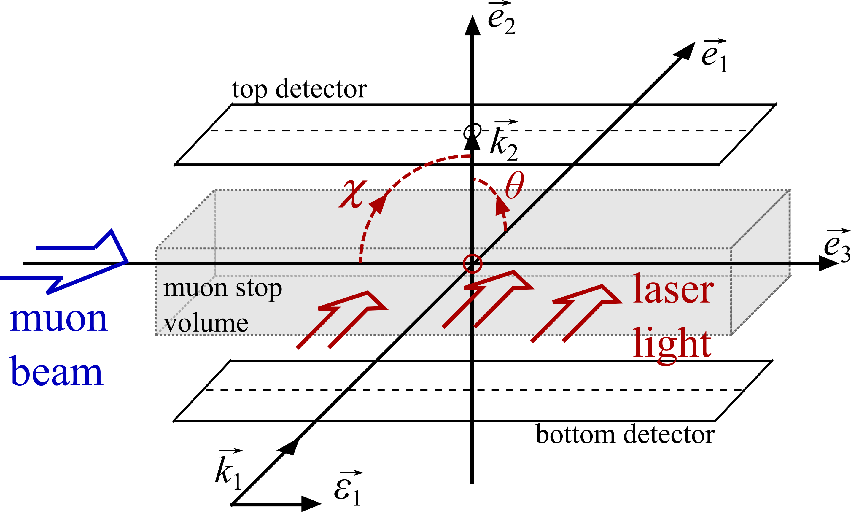
Figure 4: (Color online) Simplified view of the CREMA target volume. Muons enter the gas target from the left (blue arrow). The gray cuboid indicates the muon stop volume which is illuminated by a laser pulse propagating inside a multipass cavity (red arrows). The incoming direction and polarization are indicated by $\bm{k_{1}}$ and $\bm{\varepsilon_{1}}$. The pointlike detector assumption treats the case where the muonic atom is at the center (red circle) and the scattered photon $\bm{k_{2}}$ is emitted along $\bm{e_{2}}$ and hits the top detector in the center (black circle).

Figure 4 sketches the experimental geometry. Muonic atoms (ions) are formed in an elongated gas volume of 5$\times 12\times$190 mm³ that is illuminated from the side using a pulsed laser Antognini et al. (2005, 2009) and a multipass cavity Vogelsang et al. (2014). The $2p\rightarrow 1s$ photons emitted after laser-induced $2s\rightarrow 2p$ transitions are detected by two x-ray detectors (14$\times$150 mm² active area each) Ludhova et al. (2005); Fernandes et al. (2007); Diepold et al. (2015) placed 8 mm above and below the muon beam axis.

The simplest situation is that the $2s\rightarrow 2p$ excitation happens in the center of the target (red circle in Fig. 4), and the resulting $\bm{k_{2}}$ photon is detected in the center of the top detector (black circle). This corresponds to the pointlike detector case of $\theta=90^{\circ}$ and $\chi=90^{\circ}$ ($\delta_{\tiny\mbox{QI}}^{\perp}$ in Table 2).

However, the $2s\rightarrow 2p$ excitation takes place anywhere in the muon stop volume, and the photons of the $2p\rightarrow 1s$ decay are detected anywhere on the detectors surfaces. We consider here the laser’s propagation (${\bm{k}_{1}}$) and polarization (${\bm{\varepsilon}_{1}}$) directions being along ${\bm{e}_{1}}$ and ${\bm{e}_{3}}$, respectively. Integrating Eq. (9) over all possible angles $\chi$ accepted by the detector, while averaging over the muon stopping volume results in a considerable reduction of the observed QI effect. Again, we create pseudo data for the real geometry, fit the resonances with a simple sum of Lorentzians, and determine the resulting shift $\delta^{*}_{QI}$ of the line centers. We notice that taking into account the scattered photons at $\theta\neq 90$ ° and also the inhomogeneous muon stop probability, hardly affects the final results. As can be seen in Table 2, these shifts are much lower than the experimental accuracy of a few % of the linewidth for all muonic atoms considered here Pohl et al. (2010); Antognini et al. (2013).

IV Conclusion

We quantified the line shift caused by quantum interference for $\mu^{1}$H, $\mu^{2}$H and $\mu^{3}$He⁺ resonances, assuming first a pointlike detector. For $\mu^{1}$H, the resulting shifts are small. Hence, quantum interference cannot be the source of the proton radius puzzle, which requires a shift of the resonance in $\mu^{1}$H by four linewidths Pohl et al. (2010); Antognini et al. (2013). On the other hand, the influence of quantum interference for some resonances of $\mu^{2}$H can be as large as 12% of the linewidth for a pointlike detector.

However, we verified that even for those large QI shifts, obtained assuming a pointlike detector, the angular averaging caused by the large acceptance angle of the photon detector and the size of the muon stop volume in the CREMA experiment significantly reduces this effect to negligible values at the present level of accuracy.

Table 3: Values of the coefficients $a_{0}$, $a_{2}$ and $b_{2}$ corresponding to the parametrizations $\Lambda_{J_{i}J_{\nu}}^{F_{i}F_{\nu}}(\theta,\chi)=a_{0}+a_{2}P_{2}(\cos\gamma)$ and $\Xi_{J_{i}J_{\nu}J_{\nu^{\prime}}}^{F_{i}F_{\nu}F_{\nu^{\prime}}}(\theta,\chi)=b_{2}P_{2}(\cos\gamma)$.

$I$	$F_{i}$	$F_{\nu}$	$J_{\nu}$	$F_{\nu^{\prime}}$	$J_{\nu^{\prime}}$	$a_{0}$	$a_{2}$	$b_{2}$
1/2	0	1	1/2	1	3/2	2/81	0	-4/81
	0	1	3/2	-	-	4/81	-2/81	-
	1	1	1/2	1	3/2	4/81	0	-2/81
	1	1	1/2	2	3/2	4/81	0	-2/27
	1	1	3/2	2	3/2	2/81	1/162	-1/27
	1	2	3/2	1	3/2	10/81	-7/162	-
1	1/2	1/2	1/2	3/2	3/2	4/729	0	-8/729
	1/2	1/2	3/2	3/2	1/2	32/729	0	-32/729
	1/2	3/2	3/2	-	-	40/729	-4/729	-
	3/2	1/2	1/2	3/2	3/2	32/729	0	-32/3645
	3/2	1/2	1/2	5/2	3/2	32/729	0	-32/405
	3/2	1/2	3/2	3/2	1/2	4/729	0	-4/729
	3/2	1/2	3/2	3/2	3/2	4/729	0	16/3645
	3/2	1/2	3/2	5/2	3/2	4/729	0	-4/405
	3/2	3/2	1/2	3/2	3/2	40/729	0	-128/3645
	3/2	3/2	1/2	5/2	3/2	40/729	0	-28/405
	3/2	3/2	3/2	5/2	3/2	32/729	64/18225	-112/2025
	3/2	5/2	3/2	-	-	4/27	-28/675	-

Appendix A DIPOLE MATRIX ELEMENTS

The dipole matrix elements $D_{F^{\prime}m^{\prime}J^{\prime}}^{FmJ}$ in Eq. (2) are evaluated using standard angular reduction methods, which can start by simply expanding the product of the photon polarization and the position vector ($\bm{\varepsilon_{\gamma}}\cdot\bm{r}$) in a spherical basis, i.e.,

$$D_{F^{\prime}m^{\prime}J^{\prime}}^{FmJ} = \mathinner{\langle{\beta^{\prime}F^{\prime}m^{\prime}J^{\prime}}|}\bm{\varepsilon_{\gamma}}\cdot\bm{r}\mathinner{|{\beta FmJ}\rangle}=$$

$$\sum_{\lambda=-1}^{1}(-1)^{\lambda}\varepsilon_{\gamma}^{-\lambda}\mathinner{\langle{\beta^{\prime}F^{\prime}m^{\prime}J^{\prime}}|}r_{\lambda}\mathinner{|{\beta FmJ}\rangle}.$$

(14)

where $\beta$ contains all additional quantum numbers of the atomic state besides $F$, $m$ and $J$. Following the geometry and nomenclature of Fig. 2, the spherical form of the (normalized) polarization vectors are given by

$$\begin{array}[]{ll}\varepsilon_{l}^{(\pm 1)}=\mp\frac{(\cos\chi_{1}\pm i\sin\chi_{1})}{\sqrt{2}}~{},&\varepsilon_{l}^{(0)}=0~{},\\ \varepsilon_{2}^{(\pm 1)}=\mp\frac{(\cos\chi_{2}\cos\theta\pm i\sin\chi_{2})}{\sqrt{2}},&\varepsilon_{2}^{(0)}=-\cos\chi_{2}\sin\theta~{},\\ \end{array}$$ (15)

where $\chi\equiv\chi_{1}$.

The matrix elements of $r_{\lambda}$ can be further simplified by making use of the Wigner-Eckart theorem Rose (1957) and considering the overall atomic state being the product coupling of the nucleus and electron angular momenta, i.e.,

$$\left|\beta Fm\right\rangle=\sum_{m_{I}m_{J}}\left\langle Jm_{J}Im_{I}|Fm\right\rangle\left|Im_{I}\right\rangle\left|\beta Jm_{J}\right\rangle~{}.$$ (16)

Here, the quantities $\left\langle j_{1}m_{j_{1}}j_{2}m_{j_{2}}|j_{3}m_{j_{3}}\right\rangle$ stand for the Clebsch-Gordan coefficients. After employing sum rules of Clebsch-Gordan coefficients Rose (1957), we get

$$\left\langle\beta^{\prime}F^{\prime}m^{\prime}J^{\prime}\left|r_{\lambda}\right|\beta FmJ\right\rangle=(-1)^{F^{\prime}+I+F+1+J^{\prime}-m^{\prime}}\sqrt{[F,F^{\prime}]}\left(\begin{array}[]{ccc}F^{\prime}&1&F\\ -m^{\prime}&\lambda&m\end{array}\right)\left\{\begin{array}[]{ccc}J&I&F\\ F^{\prime}&1&J^{\prime}\end{array}\right\}\left\langle\beta^{\prime}J^{\prime}||r||\beta J\right\rangle~{},$$ (17)

where the notation $[j_{1},j_{2},...]$ is equal to $(2j_{1}+1)(2j_{2}+1)...~{}$. Since $r_{\lambda}$ does not act on the spin part of the wavefunction, the reduced matrix element $\left\langle J^{\prime}||r_{\lambda}||J_{i}\right\rangle$ is given by

$$\left\langle\beta^{\prime}J^{\prime}||r||\beta J\right\rangle=(-1)^{J^{\prime}-1/2}\sqrt{\left[J,J^{\prime}\right]}\left(\begin{array}[]{ccc}J^{\prime}&1&J\\ 1/2&0&-1/2\end{array}\right)\left\langle n^{\prime}||r||n\right\rangle~{},$$ (18)

provided that $L^{\prime}+L+1$ is even, where $L$ is the orbital angular momentum of the atomic state. Combining Eqs. (17) and (18) and rearranging the terms, the quantities $\mathcal{S}_{f\nu i}$ and $\Omega_{J_{i}J_{\nu}J_{f}}^{F_{i}F_{\nu}F_{f}}(\theta,\chi)$ of Eqs. (3) and (4) can be written as

$$\mathcal{S}_{f\nu i}=\left\langle n_{f}||r||n_{\nu}\right\rangle\left\langle n_{\nu}||r||n_{i}\right\rangle=\int r^{3}R_{f}R_{\nu}dr\int r^{3}R_{\nu}R_{i}dr=-\frac{128\sqrt{2}}{27(m_{\mu n}Z)^{2}}~{},$$ (19)

and

$$\Omega_{J_{i}J_{\nu}J_{f}}^{F_{i}F_{\nu}F_{f}}(\theta,\chi,\eta,{\bm{\varepsilon}_{2}})=[J_{\nu},F_{\nu}]\sqrt{\left[F_{f},F_{i},J_{f},J_{i}\right]}\left(\begin{array}[]{ccc}J_{f}&1&J_{\nu}\\ 1/2&0&-1/2\end{array}\right)\left(\begin{array}[]{ccc}J_{\nu}&1&J_{i}\\ 1/2&0&-1/2\end{array}\right)\left\{\begin{array}[]{ccc}F_{f}&1&F_{\nu}\\ J_{\nu}&I&J_{f}\end{array}\right\}\left\{\begin{array}[]{ccc}F_{\nu}&1&F_{i}\\ J_{i}&I&J_{\nu}\end{array}\right\}\theta_{F_{f}F_{i}}^{F_{\nu}}~{},$$ (20)

with

$$\theta_{F_{f}F_{i}}^{F_{\nu}}=\sum_{\lambda_{1},\lambda_{2}}\sum_{m_{\nu}}(-1)^{\lambda_{1}+\lambda_{2}+m_{\nu}+m_{f}+1}\hskip 2.84544pt\varepsilon_{1}^{\lambda_{1}}\varepsilon_{2}^{\lambda_{2}*}\left(\begin{array}[]{ccc}F_{f}&1&F_{\nu}\\ -m_{f}&\lambda_{2}&m_{\nu}\end{array}\right)\left(\begin{array}[]{ccc}F_{\nu}&1&F_{i}\\ -m_{\nu}&\lambda_{1}&m_{i}\end{array}\right)~{}.$$ (21)

The functions $R$ in Eq. (19) stand for the radial nonrelativistic wavefunctions, which for the case of $2s\rightarrow 2p\rightarrow 1s$ gives the numerical result shown on the right side of Eq. (19). The quantity $m_{\mu n}$ is the ratio between the muon-nucleus reduced mass and the electron mass.

In case of incident linear polarized photons, the dipole radiation pattern of the scattered photon depends only on the angle $\gamma$ between the incident polarization and the direction of the scattered photon, which is related to the previous angles by $\cos\gamma=\cos\chi\sin\theta$. $\Lambda_{J_{i}J_{\nu}}^{F_{i}F_{\nu}}(\theta,\chi)$ and $\Xi_{J_{i}J_{\nu}J_{\nu^{\prime}}}^{F_{i}F_{\nu}F_{\nu^{\prime}}}(\theta,\chi)$ are parametrized in terms of this angle $\gamma$ by $a_{0}+a_{2}P_{2}(\cos\gamma)$ and $b_{2}P_{2}(\cos\gamma)$, respectively. The respective coefficients calculated using Eq. (20) are listed in Table 3.

References

- Low (1952) F. Low, Phys. Rev., 88, 53 (1952).
- Labzowsky et al. (1994) L. Labzowsky, V. Karasiev, and I. Goidenko, J. Phys. B, 27, L439 (1994).
- Labzowsky et al. (2001) L. N. Labzowsky, D. A. Solovyev, G. Plunien, and G. Soff, Phys. Rev. Lett., 87, 143003 (2001).
- Labzowsky et al. (2009) L. Labzowsky, G. Schedrin, D. Solovyev, E. Chernovskaya, G. Plunien, and S. Karshenboim, Phys. Rev. A, 79, 052506 (2009).
- Brown et al. (2013) R. C. Brown, S. Wu, J. V. Porto, C. J. Sansonetti, C. E. Simien, S. M. Brewer, J. N. Tan, and J. D. Gillaspy, Phys. Rev. A, 87, 032504 (2013).
- Huber et al. (1999) A. Huber, B. Gross, M. Weitz, and T. W. Hänsch, Phys. Rev. A, 59, 1844 (1999).
- Niering et al. (2000) M. Niering, R. Holzwarth, J. Reichert, P. Pokasov, T. Udem, M. Weitz, T. W. Hänsch, P. Lemonde, G. Santarelli, M. Abgrall, P. Laurent, C. Salomon, and A. Clairon, Phys. Rev. Lett., 84, 5496 (2000).
- Parthey et al. (2011) C. G. Parthey, A. Matveev, J. Alnis, B. Bernhardt, A. Beyer, R. Holzwarth, A. Maistrou, R. Pohl, K. Predehl, T. Udem, T. Wilken, N. Kolachevsky, M. Abgrall, D. Rovera, C. Salomon, P. Laurent, and T. W. Hänsch, Phys. Rev. Lett., 107, 203001 (2011).
- Jentschura and Mohr (2002) U. D. Jentschura and P. J. Mohr, Can. J. Phys., 80, 633 (2002).
- Labzowsky et al. (2007) L. N. Labzowsky, G. Schedrin, D. Solovyev, and G. Plunien, Can. J. Phys., 85, 585 (2007).
- Karshenboim and Ivanov (2008) S. G. Karshenboim and V. G. Ivanov, Astron. Lett., 34, 289 (2008).
- Jentschura et al. (2003) U. D. Jentschura, J. Evers, M. Haas, and C. H. Keitel, Phys. Rev. Lett., 91, 253601 (2003).
- Franken (1961) P. A. Franken, Phys. Rev., 121, 508 (1961).
- Walkup et al. (1982) R. Walkup, A. L. Migdall, and D. E. Pritchard, Phys. Rev. A, 25, 3114 (1982).
- Sansonetti et al. (2011) C. J. Sansonetti, C. E. Simien, J. D. Gillaspy, J. N. Tan, S. M. Brewer, R. C. Brown, S. Wu, and J. V. Porto, Phys. Rev. Lett., 107, 023001 (2011).
- Horbatsch and Hessels (2010) M. Horbatsch and E. A. Hessels, Phys. Rev. A, 82, 052519 (2010).
- Marsman et al. (2012) A. Marsman, M. Horbatsch, and E. A. Hessels, Phys. Rev. A, 86, 012510 (2012a).
- Marsman et al. (2012) A. Marsman, M. Horbatsch, and E. A. Hessels, Phys. Rev. A, 86, 040501 (2012b).
- Marsman et al. (2014) A. Marsman, E. A. Hessels, and M. Horbatsch, Phys. Rev. A, 89, 043403 (2014).
- Marsman et al. (2015) A. Marsman, M. Horbatsch, and E. A. Hessels, Phys. Rev. A, 91, 062506 (2015a).
- Marsman et al. (2015) A. Marsman, M. Horbatsch, and E. A. Hessels, Journal of Physical and Chemical Reference Data, 44, 031207 (2015b).
- Yost et al. (2014) D. C. Yost, A. Matveev, E. Peters, A. Beyer, T. W. Hänsch, and T. Udem, Phys. Rev. A, 90, 012512 (2014).
- Borie (2012) E. Borie, Ann. Phys., 327, 733 (2012).
- Antognini et al. (2013) A. Antognini, F. Kottmann, F. Biraben, P. Indelicato, F. Nez, and R. Pohl, Ann. Phys., 331, 127 (2013a).
- Milotti (1998) E. Milotti, At. Data Nucl. Data Tables, 70, 137 (1998).
- Safari et al. (2012) L. Safari, P. Amaro, S. Fritzsche, J. P. Santos, S. Tashenov, and F. Fratini, Phys. Rev. A, 86, 043405 (2012).
- Safari et al. (2015) L. Safari, P. Amaro, J. P. Santos, and F. Fratini, Radiation Physics and Chemistry, 106, 271 (2015).
- Martynenko (2005) A. P. Martynenko, Phys. Rev. A, 71, 022506 (2005).
- Martynenko (2008) A. Martynenko, JETP, 106, 690 (2008).
- Borie (2005) E. Borie, Phys. Rev. A, 71, 032508 (2005).
- Pohl et al. (2010) R. Pohl, A. Antognini, F. Nez, F. D. Amaro, F. Biraben, J. M. R. Cardoso, D. S. Covita, A. Dax, S. Dhawan, L. M. P. Fernandes, A. Giesen, T. Graf, T. W. Hänsch, P. Indelicato, L. Julien, C.-Y. Kao, P. Knowles, E.-O. Le Bigot, Y.-W. Liu, J. A. M. Lopes, L. Ludhova, C. M. B. Monteiro, F. Mulhauser, T. Nebel, P. Rabinowitz, J. M. F. dos Santos, L. A. Schaller, K. Schuhmann, C. Schwob, D. Taqqu, J. F. C. A. Veloso, and F. Kottmann, Nature, 466, 213 (2010).
- Antognini et al. (2013) A. Antognini, F. Nez, K. Schuhmann, F. D. Amaro, F. Biraben, J. M. R. Cardoso, D. S. Covita, A. Dax, S. Dhawan, M. Diepold, L. M. P. Fernandes, A. Giesen, A. L. Gouvea, T. Graf, T. W. Hänsch, P. Indelicato, L. Julien, C.-Y. Kao, P. Knowles, F. Kottmann, E.-O. Le Bigot, Y.-W. Liu, J. A. M. Lopes, L. Ludhova, C. M. B. Monteiro, F. Mulhauser, T. Nebel, P. Rabinowitz, J. M. F. dos Santos, L. A. Schaller, C. Schwob, D. Taqqu, J. F. C. A. Veloso, J. Vogelsang, and R. Pohl, Science, 339, 417 (2013b).
- Antognini et al. (2011) A. Antognini, F. Biraben, J. M. R. Cardoso, D. S. Covita, A. Dax, L. M. P. Fernandes, A. L. Gouvea, T. Graf, T. W. Hänsch, M. Hildebrandt, P. Indelicato, L. Julien, K. Kirch, F. Kottmann, Y. W. Liu, C. M. B. Monteiro, F. Mulhauser, T. Nebel, F. Nez, J. M. F. dos Santos, K. Schuhmann, D. Taqqu, J. F. C. A. Veloso, A. Voss, and R. Pohl, Can. J. Phys., 89, 47 (2011).
- Nebel et al. (2012) T. Nebel, F. D. Amaro, A. Antognini, F. Biraben, J. M. R. Cardoso, D. S. Covita, A. Dax, L. M. P. Fernandes, A. L. Gouvea, T. Graf, T. W. Hänsch, M. Hildebrandt, P. Indelicato, L. Julien, K. Kirch, F. Kottmann, Y. W. Liu, C. M. B. Monteiro, F. Nez, J. M. F. d. Santos, K. Schuhmann, D. Taqqu, J. F. C. A. Veloso, A. Voss, and R. Pohl, Hyp. Int., 212, 195 (2012).
- Loudon (2000) R. Loudon, The Quantum Theory of Light (Oxford Science Publications, Oxford, 2000).
- Akhiezer and Berestetskii (1965) A. I. Akhiezer and V. B. Berestetskii, Quantum Electrodynamics (Interscience Publishers, New York, 1965).
- Safari et al. (2014) L. Safari, P. Amaro, J. P. Santos, and F. Fratini, Phys. Rev. A, 90, 014502 (2014).
- Pachucki (1996) K. Pachucki, Phys. Rev. A, 53, 2092 (1996).
- Note (1) Elliptical polarization of the incident photon can only decrease the QI shift and will be reported elsewhere.
- (40) MINUIT - Function Minimization and Error Analysis.
- Antognini et al. (2005) A. Antognini, F. D. Amaro, F. Biraben, J. M. R. Cardoso, C. A. N. Conde, D. S. Covita, A. Dax, S. Dhawan, L. M. P. Fernandes, and T. W. Hänsch, Opt. Commun., 253, 362 (2005).
- Antognini et al. (2009) A. Antognini, K. Schuhmann, F. D. Amaro, F. Biraben, A. Dax, A. Giesen, T. Graf, T. W. Hänsch, P. Indelicato, L. Julien, K. Cheng-Yang, P. E. Knowles, F. Kottmann, E. Le Bigot, L. Yi-Wei, L. Ludhova, N. Moschuring, F. Mulhauser, T. Nebel, F. Nez, P. Rabinowitz, C. Schwob, D. Taqqu, and R. Pohl, Quantum Electronics, IEEE Journal of, 45, 993 (2009).
- Vogelsang et al. (2014) J. Vogelsang, M. Diepold, A. Antognini, A. Dax, J. Götzfried, T. W. Hänsch, F. Kottmann, J. J. Krauth, Y.-W. Liu, T. Nebel, F. Nez, K. Schuhmann, D. Taqqu, and R. Pohl, Optics Express, 22, 13050 (2014).
- Ludhova et al. (2005) L. Ludhova, F. D. Amaro, A. Antognini, F. Biraben, J. M. R. Cardoso, C. A. N. Conde, D. S. Covita, A. Dax, S. Dhawan, L. M. P. Fernandes, T. W. Hänsch, V. W. Hughes, O. Huot, P. Indelicato, L. Julien, P. E. Knowles, F. Kottmann, J. A. M. Lopes, Y. W. Liu, C. M. B. Monteiro, F. Mulhauser, F. Nez, R. Pohl, P. Rabinowitz, J. M. F. dos Santos, L. A. Schaller, D. Taqqu, and J. F. C. A. Veloso, Nucl. Instrum. and Meth. Phys. A, 540, 169 (2005).
- Fernandes et al. (2007) L. M. P. Fernandes, F. D. Amaro, A. Antognini, J. M. R. Cardoso, C. A. N. Conde, O. Huot, P. E. Knowles, F. Kottmann, J. A. M. Lopes, L. Ludhova, C. M. B. Monteiro, F. Mulhauser, R. Pohl, J. M. F. d. Santos, L. A. Schaller, D. Taqqu, and J. F. C. A. Veloso, Journal of Instrumentation, 2, P08005 (2007).
- Diepold et al. (2015) M. Diepold, L. M. P. Fernandes, J. Machado, P. Amaro, M. Abdou-Ahmed, F. D. Amaro, A. Antognini, F. Biraben, T.-L. Chen, D. S. Covita, A. J. Dax, B. Franke, S. Galtier, A. L. Gouvea, J. Götzfried, T. Graf, T. W. Hänsch, M. Hildebrandt, P. Indelicato, L. Julien, K. Kirch, A. Knecht, F. Kottmann, J. J. Krauth, Y.-W. Liu, C. M. B. Monteiro, F. Mulhauser, B. Naar, T. Nebel, F. Nez, J. P. Santos, J. M. F. dos Santos, K. Schuhmann, C. I. Szabo, D. Taqqu, J. F. C. A. Veloso, A. Voss, B. Weichelt, and R. Pohl, Rev. Sci. Instrum., 86, 053102 (2015).
- Rose (1957) M. E. Rose, Elementary Theory of Angular Momentum (John Wiley, New York, 1957).