Selective Greedy Equivalence Search: Finding Optimal Bayesian Networks Using a Polynomial Number of Score Evaluations

Abstract

We introduce Selective Greedy Equivalence Search (SGES), a restricted version of Greedy Equivalence Search (GES). SGES retains the asymptotic correctness of GES but, unlike GES, has polynomial performance guarantees. In particular, we show that when data are sampled independently from a distribution that is perfect with respect to a DAG ${\cal G}$ defined over the observable variables then, in the limit of large data, SGES will identify ${\cal G}$’s equivalence class after a number of score evaluations that is (1) polynomial in the number of nodes and (2) exponential in various complexity measures including maximum-number-of-parents, maximum-clique-size, and a new measure called v-width that is at least as small as—and potentially much smaller than—the other two. More generally, we show that for any hereditary and equivalence-invariant property $\Pi$ known to hold in ${\cal G}$, we retain the large-sample optimality guarantees of GES even if we ignore any GES deletion operator during the backward phase that results in a state for which $\Pi$ does not hold in the common-descendants subgraph.

1 INTRODUCTION

Greedy Equivalence Search (GES) is a score-based search algorithm that searches over equivalence classes of Bayesian-network structures. The algorithm is appealing because (1) for finite data, it explicitly (and greedily) tries to maximize the score of interest, and (2) as the data grows large, it is guaranteed—under suitable distributional assumptions—to return the generative structure. Although empirical results show that the algorithm is efficient in real-world domains, the number of search states that GES needs to evaluate in the worst case can be exponential in the number of domain variables.

In this paper, we show that if we assume the generative distribution is perfect with respect to some DAG ${\cal G}$ defined over the observable variables, and if ${\cal G}$ is known to be constrained by various graph-theoretic measures of complexity, then we can disregard all but a polynomial number of the backward search operators considered by GES while retaining the large-sample guarantees of the algorithm; we call this new variant of GES selective greedy equivalence search or SGES. Our complexity results are a consequence of a new understanding of the backward phase of GES, in which edges (either directed or undirected) are greedily deleted from the current state until a local minimum is reached. We show that for any hereditary and equivalence-invariant property known to hold in generative model ${\cal G}$, we can remove from consideration any edge-deletion operator between $X$ and $Y$ for which the property does not hold in the resulting induced subgraph over $X,$ $Y,$ and their common descendants. As an example, if we know that each node has at most $k$ parents, we can remove from consideration any deletion operator that results in a common child with more than $k$ parents.

We define a new notion of complexity that we call v-width. For a given generative structure ${\cal G}$, v-width is necessarily smaller than the maximum clique size, which is necessarily smaller than or equal to the maximum number of parents per node. By casting limited v-width and other complexity constraints as graph properties, we show how to enumerate directly over a polynomial number of edge-deletion operators at each step, and we show that we need only a polynomial number of calls to the scoring function to complete the algorithm.

The main contributions of this paper are theoretical. Our definition of the new SGES algorithm deliberately leaves unspecified the details of how to implement its forward phase; we prove our results for SGES given any implementation of this phase that completes with a polynomial number of calls to the scoring function. A naive implementation is to immediately return a complete (i.e., no independence) graph using no calls to the scoring function, but this choice is unlikely to be reasonable in practice, particularly in discrete domains where the sample complexity of this initial model will likely be a problem. Whereas we believe it an important direction, our paper does not explore practical alternatives for the forward phase that have polynomial-time guarantees.

This paper, which is an expanded version of Chickering and Meek (2015) and includes all proofs, is organized as follows. In Section 2, we describe related work. In Section 3, we provide notation and background material. In Section 4, we present our new SGES algorithm, we show that it is optimal in the large-sample limit, and we provide complexity bounds when given an equivalence-invariant and hereditary property that holds on the generative structure. In Section 5, we present a simple synthetic experiment that demonstrates the value of restricting the backward operators in SGES. We conclude with a discussion of our results in Section 6.

2 RELATED WORK

It is useful to distinguish between approaches to learning the structure of graphical models as constraint based, score based or hybrid. Constraint-based approaches typically use (conditional) independence tests to eliminate potential models, whereas score-based approaches typically use a penalized likelihood or a marginal likelihood to evaluate alternative model structures; hybrid methods combine these two approaches. Because score-based approaches are driven by a global likelihood, they are less susceptible than constraint-based approaches to incorrect categorical decisions about independences.

There are polynomial-time algorithms for learning the best model in which each node has at most one parent. In particular, the Chow-Liu algorithm (Chow and Liu, 1968) used with any equivalence-invariant score will identify the highest-scoring tree-like model in polynomial time; for scores that are not equivalence invariant, we can use the polynomial-time maximum-branching algorithm of Edmonds (1967) instead. Gaspers et al. (2012) show how to learn k-branchings in polynomial time; these models are polytrees that differ from a branching by a constant $k$ number of edge deletions.

Without additional assumptions, most results for learning non-tree-like models are negative. Meek (2001) shows that finding the maximum-likelihood path is NP-hard, despite this being a special case of a tree-like model. Dasgupta (1999) shows that finding the maximum-likelihood polytree (a graph in which each pair of nodes is connected by at most one path) is NP-hard, even with bounded in-degree for every node. For general directed acyclic graphs, Chickering (1996) shows that finding the highest marginal-likelihood structure under a particular prior is NP-hard, even when each node has at most two parents. Chickering at al. (2004) extend this same result to the large-sample case.

Researchers often assume that the training-data “generative” distribution is perfect with respect to some model class in order to reduce the complexity of learning algorithms. Geiger et al. (1990) provide a polynomial-time constraint-based algorithm for recovering a polytree under the assumption that the generative distribution is perfect with respect to a polytree; an analogous score-based result follows from this paper. The constraint-based PC algorithm of Sprites et al. (1993) can identify the equivalence class of Bayesian networks in polynomial time if the generative structure is a DAG model over the observable variables in which each node has a bounded degree; this paper provides a similar result for a score-based algorithm. Kalish and Buhlmann (2007) show that for Gaussian distributions, the PC algorithm can identify the right structure even when the number of nodes in the domain is larger than the sample size. Chickering (2002) uses the same DAG-perfectness-over-observables assumption to show that the greedy GES algorithm is optimal in the large-sample limit, although the branching factor of GES is worst-case exponential; the main result of this paper shows how to limit this branching factor without losing the large-sample guarantee. Chickering and Meek (2002) show that GES identifies a “minimal” model in the large-sample limit under a less restrictive set of assumptions.

Hybrid methods for learning DAG models use a constraint-based algorithm to prune out a large portion of the search space, and then use a score-based algorithm to select among the remaining (Friedman et al., 1999; Tsamardinos et al., 2006). Ordyniak and Szeider (2013) give positive complexity results for the case when the remaining DAGs are characterized by a structure with constant treewidth.

Many researchers have turned to exhaustive enumeration to identify the highest-scoring model (Gillispie and Perlman, 2001; Koivisto and Sood 2004; Silander and Myllymäki, 2006; Kojima et al, 2010). There are many complexity results for other model classes. Karger and Srebro (2001) show that finding the optimal Markov network is NP-complete for treewidth $>1$. Narasimhan and Bilmes (2004) and Shahaf, Chechetka and Guestrin (2009) show how to learn approximate limited-treewidth models in polynomial time. Abeel, Koller and Ng (2005) show how to learn factor graphs in polynomial time.

3 NOTATION AND BACKGROUND

We use the following syntactical conventions in this paper. We denote a variable by an upper case letter (e.g., $A$) and a state or value of that variable by the same letter in lower case (e.g., $a$). We denote a set of variables by a bold-face capitalized letter or letters (e.g., ${\bf X}$). We use a corresponding bold-face lower-case letter or letters (e.g., ${\bf x}$) to denote an assignment of state or value to each variable in a given set. We use calligraphic letters (e.g., ${\cal G},\mbox{$\cal E$}$) to denote statistical models and graphs.

A Bayesian-network model for a set of variables ${\bf U}$ is a pair $({\cal G},\mbox{\boldmath$\theta$})$. ${\cal G}=({\bf V,E})$ is a directed acyclic graph—or DAG for short—consisting of nodes in one-to-one correspondence with the variables and directed edges that connect those nodes. $\theta$ is a set of parameter values that specify all of the conditional probability distributions. The Bayesian network represents a joint distribution over ${\bf U}$ that factors according to the structure ${\cal G}$.

The structure ${\cal G}$ of a Bayesian network represents the independence constraints that must hold in the distribution. The set of all independence constraints implied by the structure ${\cal G}$ can be characterized by the Markov conditions, which are the constraints that each variable is independent of its non-descendants given its parents. All other independence constraints follow from properties of independence. A distribution defined over the variables from ${\cal G}$ is perfect with respect to ${\cal G}$ if the set of independences in the distribution is equal to the set of independences implied by the structure ${\cal G}$.

Two DAGs ${\cal G}$ and ${\cal G}^{\prime}$ are equivalent—denoted ${\cal G}\approx{\cal G}^{\prime}$—if the independence constraints in the two DAGs are identical. Because equivalence is reflexive, symmetric, and transitive, the relation defines a set of equivalence classes over network structures. We will use $[{\cal G}]_{\approx}$ to denote the equivalence class of DAGs to which ${\cal G}$ belongs.

An equivalence class of DAGs $\cal F$ is an independence map (IMAP) of another equivalence class of DAGs $\cal E$ if all independence constraints implied by $\cal F$ are also implied by $\cal E$. For two DAGs ${\cal G}$ and ${\cal H}$, we use ${\cal G}\leq{\cal H}$ to denote that $[{\cal H}]_{\approx}$ is an IMAP of $[{\cal G}]_{\approx}$; we use ${\cal G}<{\cal H}$ when ${\cal G}\leq{\cal H}$ and $\mbox{$[{\cal H}]_{\approx}$}\not=\mbox{$[{\cal G}]_{\approx}$}$.

As shown by Verma and Pearl (1991), two DAGs are equivalent if and only if they have the same skeleton (i.e., the graph resulting from ignoring the directionality of the edges) and the same v-structures (i.e., pairs of edges $X\rightarrow Y$ and $Y\leftarrow Z$ where $X$ and $Z$ are not adjacent). As a result, we can use a partially directed acyclic graph—or PDAG for short—to represent an equivalence class of DAGs: for a PDAG $\cal P$, the equivalence class of DAGs is the set that share the skeleton and v-structures with $\cal P$.

We extend our notation for DAG equivalence and the DAG IMAP relation to include the more general PDAG structure. In particular, for a PDAG $\cal P$, we use $[\mbox{$\cal P$}]_{\approx}$ to denote the corresponding equivalence class of DAGs. For any pair of PDAGs $\cal P$ and $\cal Q$—where one or both may be a DAG—we use $\mbox{$\cal P$}\approx\mbox{$\cal Q$}$ to denote $\mbox{$[\mbox{$\cal Q$}]_{\approx}$}=\mbox{$[\mbox{$\cal P$}]_{\approx}$}$ and we use $\mbox{$\cal P$}\leq\mbox{$\cal Q$}$ to denote $[\mbox{$\cal Q$}]_{\approx}$ is an IMAP of $[\mbox{$\cal P$}]_{\approx}$. To avoid confusion, for the remainder of the paper we will reserve the symbols ${\cal G}$ and ${\cal H}$ for DAGs.

For any PDAG $\cal P$ and subset of nodes ${\bf V}$, we use $\mbox{$\cal P$}[\mbox{${\bf V}$}]$ to denote the subgraph of $\cal P$ induced by ${\bf V}$; that is, $\mbox{$\cal P$}[\mbox{${\bf V}$}]$ has as nodes the set ${\bf V}$ and has as edges all those from $\cal P$ that connect nodes in ${\bf V}$. We use ${\bf NA}_{X,Y}$ to denote, within a PDAG, the set of nodes that are neighbors of $X$ (i.e., connected with an undirected edge) and also adjacent to $Y$ (i.e., without regard to whether the connecting edge is directed or undirected).

An edge in ${\cal G}$ is compelled if it exists in every DAG that is equivalent to ${\cal G}$. If an edge in ${\cal G}$ is not compelled, we say that it is reversible. A completed PDAG (CPDAG) ${\cal C}$ is a PDAG with two additional properties: (1) for every directed edge in ${\cal C}$, the corresponding edge in ${\cal G}$ is compelled and (2) for every undirected edge in ${\cal C}$ the corresponding edge in ${\cal G}$ is reversible. Unlike non-completed PDAGs, the CPDAG representation of an equivalence class is unique. We use ${\bf Pa}^{\mbox{$\cal P$}}_{Y}$ to denote the parents of node $Y$ in $\cal P$. An edge $X\rightarrow Y$ is covered in a DAG if $X$ and $Y$ have the same parents, with the exception that $X$ is not a parent of itself.

3.1 Greedy Equivalence Search

 Algorithm $GES(\mbox{${\bf D}$})$  Input : Data ${\bf D}$

Output : CPDAG ${\cal C}$

$\mbox{${\cal C}$}\longleftarrow$ FES(${\bf D}$)

$\mbox{${\cal C}$}\longleftarrow$ BES(${\bf D}$, ${\cal C}$)

return ${\cal C}$

 

Algorithm 1 Pseudo-code for the GES algorithm.

The GES algorithm, shown in Figure 1, performs a two-phase greedy search through the space of DAG equivalence classes. GES represents each search state with a CPDAG, and performs transformation operators to this representation to traverse between states. Each operator corresponds to a DAG edge modification, and is scored using a DAG scoring function that we assume has three properties. First, we assume the scoring function is score equivalent, which means that it assigns the same score to equivalent DAGs. Second, we assume the scoring function is locally consistent, which means that, given enough data, (1) if the current state is not an IMAP of ${\cal G}$, the score prefers edge additions that remove incorrect independences, and (2) if the current state is an IMAP of ${\cal G}$, the score prefers edge deletions that remove incorrect dependences. Finally, we assume the scoring function is decomposable, which means we can express it as:

$$Score({\cal G},\mbox{${\bf D}$})=\sum_{i=1}^{n}Score(X_{i},\mbox{${\bf Pa}^{{\cal G}}_{i}$})$$ (1)

Note that the data ${\bf D}$ is implicit in the right-hand side Equation 1. Most commonly used scores in the literature have these properties. For the remainder of this paper, we assume they hold for the scoring function we use.

All of the CPDAG operators from GES are scored using differences in the DAG scoring function, and in the limit of large data, these scores are positive precisely for those operators that remove incorrect independences and incorrect dependences.

The first phase of the GES—called forward equivalence search or FES—starts with an empty (i.e., no-edge) CPDAG and greedily applies GES insert operators until no operator has a positive score; these operators correspond precisely to the union of all single-edge additions to all DAG members of the current (equivalence-class) state. After FES reaches a local maximum, GES switches to the second phase—called backward equivalence search or BES—and greedily applies GES delete operators until no operator has a positive score; these operators correspond precisely to the union of all single-edge deletions from all DAG members of the current state.

Theorem 1.

(Chickering, 2002) Let ${\cal C}$ be the CPDAG that results from applying the GES algorithm to $m$ records sampled from a distribution that is perfect with respect to DAG ${\cal G}$. Then in the limit of large $m$, $\mbox{${\cal C}$}\approx{\cal G}$.

The role of FES in the large-sample limit is only to identify a state ${\cal C}$ for which ${\cal G}\leq\mbox{${\cal C}$}$; Theorem 1 holds for GES under any implementation of FES that results in an IMAP of ${\cal G}$. The implementation details can be important in practice because what constitutes a “large” amount of data depends on the number of parameters in the model. In theory, however, we could simply replace FES with a (constant-time) algorithm that sets ${\cal C}$ to be the no-independence equivalence class.

The focus of our analysis in the next section is on a modified version of BES, and the details of the delete operator used in this phase are important. We detail the preconditions, scoring function, and transformation algorithm for a delete operator in Figure 2. We note that we do not need to make any CPDAG transformations when scoring the operators; it is only once we have identified the highest-scoring (non-negative) delete that we need to make the transformation shown in the figure. After applying the edge modifications described in the foreach loop, the resulting PDAG $\cal P$ is not necessarily completed and hence we may have to convert $\cal P$ into the corresponding CPDAG representation. As shown by Chickering (2002), this conversion can be accomplished easily by using the structure of $\cal P$ to extract a DAG that we then convert into a CPDAG by undirecting all reversible edges. The complexity of this procedure for a $\cal P$ with $n$ nodes and $e$ edges is $O(n\cdot e)$, and requires no calls to the scoring function.

 Operator:    $Delete(X,Y,\mbox{${\bf H}$})$ applied to ${\cal C}$  $\bullet$ Preconditions

$X$ and $Y$ are adjacent

$\mbox{${\bf H}$}\subseteq{\bf NA}_{Y,X}$

$\overline{\mbox{${\bf H}$}}={\bf NA}_{Y,X}\setminus\mbox{${\bf H}$}$ is a clique

$\bullet$ Scoring

$Score(Y,\{\mbox{${\bf Pa}^{\mbox{${\cal C}$}}_{Y}$}\cup\overline{\mbox{${\bf H}$}}\}\setminus X)-Score(Y,X\cup\mbox{${\bf Pa}^{\mbox{${\cal C}$}}_{Y}$}\cup\overline{\mbox{${\bf H}$}})$

$\bullet$ Transformation

Remove edge between $X$ and $Y$

foreach $H\in\mbox{${\bf H}$}$ do

     Replace $Y-H$ with $Y\rightarrow H$

      if $X-H$ then Replace with $X\rightarrow H$;

     

      end foreach

     Convert to CPDAG

 

Figure 2 Preconditions, scoring, and transformation algorithm for a delete operator applied to a CPDAG.

4 SELECTIVE GREEDY EQUIVALENCE SEARCH

In this section, we define a variant of the GES algorithm called selective GES—or SGES for short—that uses a subset of the GES operators. The subset is chosen based on a given property $\Pi$ that is known to hold for the generative structure ${\cal G}$. Just like GES, SGES—shown in Figure 3—has a forward phase and a backward phase.

For the forward phase of SGES, it suffices for our theoretical analysis that we use a method that returns an IMAP of ${\cal G}$ (in the large-sample limit) using only a polynomial number of insert-operator score calls. For this reason, we call this phase poly-FES. A simple implementation of poly-FES is to return the no-independence CPDAG (with no score calls), but other implementations are likely more useful in practice.

The backward phase of SGES—which we call selective backward equivalence search (SBES)—uses only a subset of the BES delete operators. This subset must necessarily include all $\Pi$-consistent delete operators—defined below—in order to maintain the large-sample consistency of GES, but the subset can (and will) include additional operators for the sake of efficient enumeration.

The DAG properties used by SGES must be equivalence invariant, meaning that for any pair of equivalent DAGs, either the property holds for both of them or it holds for neither of them. Thus, for any equivalence-invariant DAG property $\Pi$, it makes sense to say that $\Pi$ either holds or does not hold for a PDAG. As shown by Chickering (1995), a DAG property is equivalence invariant if and only if it is invariant to covered-edge reversals; it follows that the property that each node has at most $k$ parents is equivalence invariant, whereas the property that the length of the longest directed path is at least $k$ is not. Furthermore, the properties for SGES must also be hereditary, which means that if $\Pi$ holds for a PDAG $\cal P$ it must also hold for all induced subgraphs of $\cal P$. For example, the max-parent property is hereditary, whereas the property that each node has at least $k$ parents is not. We use EIH property to refer to a property that is equivalence invariant and hereditary.

Definition 1.

$\Pi$-Consistent GES Delete
A GES delete operator $Delete(X,Y,\mbox{${\bf H}$})$ is $\Pi$ consistent for CPDAG ${\cal C}$ if, for the set of common descendants ${\bf W}$ of $X$ and $Y$ in the resulting CPDAG $\mbox{${\cal C}$}^{\prime}$, the property holds for the induced subgraph $\mbox{${\cal C}$}^{\prime}[X\cup Y\cup\mbox{${\bf W}$}]$.

In other words, after the delete, the property holds for the subgraph defined by $X$, $Y$, and their common descendants.

 Algorithm $SGES(\mbox{${\bf D}$},\Pi)$  Input : Data ${\bf D}$, Property $\Pi$

Output : CPDAG ${\cal C}$

$\mbox{${\cal C}$}\longleftarrow$ poly-FES

$\mbox{${\cal C}$}\longleftarrow$ SBES(${\bf D}$, ${\cal C}$, $\Pi$)

return ${\cal C}$

 

Algorithm 3 Pseudo-code for the SGES algorithm.

 Algorithm $SBES(\mbox{${\bf D}$},\mbox{${\cal C}$},\Pi)$  Input : Data ${\bf D}$, CPDAG ${\cal C}$, Property $\Pi$

Output :  CPDAG

Repeat

${\bf Ops}\longleftarrow$ Generate $\Pi$-consistent delete operators for ${\cal C}$

$Op\longleftarrow$ highest-scoring operator in ${\bf Ops}$

if score of $Op$ is negative then return ${\cal C}$

$\mbox{${\cal C}$}\longleftarrow$ Apply $Op$ to ${\cal C}$

 

Algorithm 4 Pseudo-code for the SBES algorithm.

4.1 LARGE-SAMPLE CORRECTNESS

The following theorem establishes a graph-theoretic justification for considering only the $\Pi$-consistent deletions at each step of SBES.

Theorem 2.

If ${\cal G}<\mbox{${\cal C}$}$ for CPDAG ${\cal C}$ and DAG ${\cal G}$, then for any EIH property $\Pi$ that holds on ${\cal G}$, there exists a $\Pi$-consistent $Delete(X,Y,\mbox{${\bf H}$})$ that when applied to ${\cal C}$ results in the CPDAG $\mbox{${\cal C}$}^{\prime}$ for which ${\cal G}\leq\mbox{${\cal C}$}^{\prime}$.

We postpone the proof of Theorem 2 to the appendix. The result is a consequence of an explicit characterization of, for a given pair of DAGs ${\cal G}$ and ${\cal H}$ such that ${\cal G}<{\cal H}$, an edge in ${\cal H}$ that we can either reverse or delete in ${\cal H}$ such that for the resulting DAG ${\cal H}^{\prime}$, we have ${\cal G}\leq{\cal H}^{\prime}$.

Theorem 3.

Let ${\cal C}$ be the CPDAG that results from applying the SGES algorithm to (1) $m$ records sampled from a distribution that is perfect with respect to DAG ${\cal G}$ and (2) EIH property $\Pi$ that holds on ${\cal G}$. Then in the limit of large $m$, $\mbox{${\cal C}$}\approx{\cal G}$.

Proof: Because the scoring function is locally consistent, we know poly-FES must return an IMAP of ${\cal G}$. Because SBES includes all the $\Pi$-consistent delete operators, Theorem 2 guarantees that, unless $\mbox{${\cal C}$}\approx{\cal G}$, there will be a positive-scoring operator. ∎

4.2 COMPLEXITY MEASURES

In this section, we discuss a number of distributional assumptions that we can use with Theorem 3 to limit the number of operators that SGES needs to score. As discussed in Section 2, when we assume the generative distribution is perfect with respect to a DAG ${\cal G}$, then graph-theoretic assumptions about ${\cal G}$ can lead to more efficient training algorithms. Common assumptions used include (1) a maximum parent-set size for any node, (2) a maximum-clique size among any nodes and (3) a maximum treewidth. Treewidth is important because the complexity of exact inference is exponential in this measure.

We can associate a property with each of these assumptions that holds precisely when the DAG ${\cal G}$ satisfies that assumption. Consider the constraint that the maximum number of parents for any node in ${\cal G}$ is some constant $k$. Then, using “PS” to denote parent size, we can define the property $\Pi_{PS}^{k}$ to be true precisely for those DAGs in which each node has at most $k$ parents. Similarly we can define $\Pi_{CL}^{k}$ and $\Pi_{TW}^{k}$ to correspond to maximum-clique size and maximum treewidth, respectively.

For two properties $\Pi$ and $\Pi^{\prime}$, we write $\Pi\subseteq\Pi^{\prime}$ if for every DAG ${\cal G}$ for which $\Pi$ holds, $\Pi^{\prime}$ also holds. In other words, $\Pi$ is a more constraining property than is $\Pi^{\prime}$. Because the lowest node in any clique has all other nodes in the clique as parents, it is easy to see that $\Pi_{PS}^{k}\subseteq\Pi_{CL}^{k-1}$. Because the treewidth for DAG ${\cal G}$ is defined to be the size of the largest clique minus one in a graph whose cliques are at least as large as those in ${\cal G}$, we also have $\Pi_{TW}^{k}\subseteq\Pi_{CL}^{k-1}$. Which property to use will typically be a trade-off between how reasonable the assumption is (i.e, less constraining properties are more reasonable) and the efficiency of the resulting algorithm (i.e., more constraining properties lead to faster algorithms).

We now consider a new complexity measure called v-width, whose corresponding property is less constraining than the previous three, and somewhat remarkably leads to an efficient implementation in SGES. For a DAG ${\cal G}$, the v-width is defined to be the maximum of, over all pairs of non-adjacent nodes $X$ and $Y$, the size of the largest clique among common children of $X$ and $Y$. In other words, v-width is similar to the maximum-clique-size bound, except that the bound only applies to cliques of nodes that are shared children of some pair of non-adjacent nodes. With this understanding it is easy to see that, for the property $\Pi_{VW}^{k}$ corresponding to a bound on the v-width, we have $\Pi_{CL}^{k}\subseteq\Pi_{VW}^{k}$.

To illustrate the difference between v-width and the other complexity measures, consider the two DAGs in Figure 1. The DAG in Figure 1(a) has a clique of size $K$, and consequently a maximum-clique size of $K$ and a maximum parent-set size of $K-1$. Thus, if $K$ is $O(n)$ for a large graph of $n$ nodes, any algorithm that is exponential in these measures will not be efficient. The v-width, however, is zero for this DAG. The DAG in Figure 1(b), on the other hand, has a v-width of $K$.

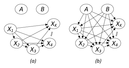
Figure 1: Two DAGs (a) and (b) having identical maximum clique sizes, similar maximum number of parents, and divergent v-widths.

In order to use a property with SGES, we need to establish that it is EIH. For $\Pi_{PS}^{k}$, $\Pi_{CL}^{k}$ and $\Pi_{VW}^{k}$, equivalence-invariance follows from the fact that all three properties are covered-edge invariant, and hereditary follows because the corresponding measures cannot increase when we remove nodes and edges from a DAG. Although we can establish EIH for the treewidth property $\Pi_{TW}^{k}$ with more work, we omit further consideration of treewidth for the sake of space.

4.3 GENERATING DELETIONS

In this section, we show how to generate a set of deletion operators for SBES such that all $\Pi$-consistent deletion operators are included, for any $\Pi\in\{\Pi_{PS}^{k},\Pi_{CL}^{k},\Pi_{VW}^{k}\}$. Furthermore, the total number of deletion operators we generate is polynomial in the number of nodes in the domain and exponential in $k$.

Our approach is to restrict the $Delete(X,Y,\mbox{${\bf H}$})$ operators based on the ${\bf H}$ sets and the resulting CPDAG $\mbox{${\cal C}$}^{\prime}$. In particular, we rule out candidate ${\bf H}$ sets for which $\Pi$ does not hold on the induced subgraph $\mbox{${\cal C}$}^{\prime}[\mbox{${\bf H}$}\cup X\cup Y]$; because all nodes in ${\bf H}$ will be common children of $X$ and $Y$ in $\mbox{${\cal C}$}^{\prime}$—and thus a subset of the common descendants of $X$ and $Y$—we know from Definition 1 (and the fact that $\Pi$ is hereditary) that none of the dropped operators can be $\Pi$-consistent.

Before presenting our restricted-enumeration algorithm, we now discuss how to enumerate delete operators without restrictions. As shown by Andersson et al. (1997), a CPDAG is a chain graph whose undirected components are chordal. This means that the induced sub-graph defined over ${\bf NA}_{Y,X}$—which is a subset of the neighbors of $Y$—is an undirected chordal graph. A useful property of chordal graphs is that we can identify, in polynomial time, a set of maximal cliques over these nodes; let $\mbox{${\bf C}$}_{1},...,\mbox{${\bf C}$}_{m}$ denote the nodes contained within these $m$ maximal cliques, and let $\overline{\mbox{${\bf H}$}}={\bf NA}_{Y,X}\setminus\mbox{${\bf H}$}$ be the complement of the shared neighbors with respect to the candidate ${\bf H}$. Recall from Figure 2 that the preconditions for any $Delete(X,Y,\mbox{${\bf H}$})$ include the requirement that $\overline{\mbox{${\bf H}$}}$ is a clique. This means that for any valid ${\bf H}$, there must be some maximal clique $\mbox{${\bf C}$}_{i}$ that contains the entirety of $\overline{\mbox{${\bf H}$}}$; thus, we can generate all operators (without regard to any property) by stepping through each maximal clique $\mbox{${\bf C}$}_{i}$ in turn, initializing ${\bf H}$ to be all nodes not in $\mbox{${\bf C}$}_{i}$, and then generating a new operator corresponding to expanding ${\bf H}$ by all subsets of nodes in $\mbox{${\bf C}$}_{i}$. Note that if ${\bf NA}_{Y,X}$ is itself a clique, we are enumerating over all $2^{|{\bf NA}_{Y,X}|}$ operators.

As we show below, all three of the properties of interest impose a bound on the maximum clique size among nodes in ${\bf H}$. If we are given such a bound $s$, we know that any “expansion” subset for a clique that has size greater than $s$ will result in an operator that is not valid. Thus, we can implement the above operator-enumeration approach more efficiently by only generating subsets within each clique that have size at most $s$. This allows us to process each clique $\mbox{${\bf C}$}_{i}$ with only $O(|\mbox{${\bf C}$}_{i}+1|^{s})$ calls to the scoring function. In addition, we need not enumerate over any of the subsets of $\mbox{${\bf C}$}_{i}$ if, after removing this clique from the graph, there remains a clique of size greater than $s$; we define the function $FilterCliques(\{\mbox{${\bf C}$}_{1},\ldots,\mbox{${\bf C}$}_{m}\},s)$ to be the subset of cliques that remain after imposing this constraint. With this function, we can define Selective-Generate-Ops as shown in Figure 5 to leverage the max-clique-size constraint when generating operators; this algorithm will in turn be used to generate all of the CPDAG operators during SBES.

Example: In Figure 2, we show an example CPDAG for which to run Selective-Generate-Ops(${\cal C}$, $X$, $Y$, $s$) for various values of $s$. In the example, there is a single clique $\mbox{${\bf C}$}=\{A,B\}$ in the set ${\bf NA}_{Y,X}$, and thus at the top of the outer foreach loop, the set $\mbox{${\bf H}$}_{0}$ is initialized to the empty set. If $s=0$, the only subset of ${\bf C}$ with size zero is the empty set, and so that is added to ${\bf Ops}$ and the algorithm returns. If $s=1$ we add, in addition to the empty set, all singleton subsets of ${\bf C}$. For $s\geq 2$, we add all subsets of ${\bf C}$. ∎

Now we discuss how each of the three properties impose a constraint $s$ on the maximum clique among nodes in ${\bf H}$, and consequently the selective-generation algorithm in Figure 5 can be used with each one, given an appropriate bound $s$. For both $\Pi_{VW}^{k}$ and $\Pi_{CL}^{k}$, the $k$ given imposes an explicit bound on $s$ (i.e., $s=k$ for both). Because any clique in ${\bf H}$ of size $r$ will result in a DAG member of the resulting equivalence class having a node in that clique with at least $r+1$ parents (i.e., $r-1$ from the other nodes in the clique, plus both $X$ and $Y$), we have for $\Pi_{PS}^{k}$, $s=k-1$.

 Algorithm Selective-Generate-Ops($\mbox{${\cal C}$},X,Y,s$)  Input : CPDAG ${\cal C}$ with adjacent $X$,$Y$ and limit $s$

Output : ${\bf Ops}=\{\mbox{${\bf H}$}_{1},\ldots,\mbox{${\bf H}$}_{m}$}

${\bf Ops}\longleftarrow\emptyset$

Generate maximal cliques $\mbox{${\bf C}$}_{1},...,\mbox{${\bf C}$}_{m}$ from ${\bf NA}_{Y,X}$

$\mbox{${\bf S}$}\longleftarrow FiltertCliques(\{\mbox{${\bf C}$}_{1},\ldots,\mbox{${\bf C}$}_{m}\},s)$

foreach $\mbox{${\bf C}$}_{i}\in\mbox{${\bf S}$}$ do

      $\mbox{${\bf H}$}_{0}\longleftarrow{\bf NA}_{Y,X}\setminus\mbox{${\bf C}$}_{i}$

      foreach $\mbox{${\bf C}$}\subseteq\mbox{${\bf C}$}_{i}$ with $|\mbox{${\bf C}$}|\leq s$ do

           Add $\mbox{${\bf H}$}_{0}\cup\mbox{${\bf C}$}$ to ${\bf Ops}$

           end foreach

          

           end foreach

          return ${\bf Ops}$

 

Algorithm 5 Algorithm to generate clique-size limited delete operators.

We summarize the discussion above in the following proposition.

Proposition 1.

Algorithm Selective-Generate-Ops applied to all edges using clique-size bound $s$ generates all $\Pi$-consistent delete operators for $\Pi\in\{\Pi_{PS}^{s+1},\Pi_{CL}^{s},\Pi_{VW}^{s}\}$.

We now argue that running SBES on a domain of $n$ variables when using Algorithm Selective-Generate-Ops with a bound $s$ requires only a polynomial number in $n$ of calls to the scoring function. Each clique in the inner loop of the algorithm can contain at most $n$ nodes, and therefore we generate and score at most $(n+1)^{s}$ operators, requiring at most $2(n+1)^{s}$ calls to the scoring function. Because the cliques are maximal, there can be at most $n$ of them considered in the outer loop. Because there are never more than $n^{2}$ edges in a CPDAG, and we will delete at most all of them, we conclude that even if we decided to rescore every operator after every edge deletion, we will only make a polynomial number of calls to the scoring function.

From the above discussion and the fact that SBES completes using at most a polynomial number of calls to the scoring function, we get the following result for the full SGES algorithm.

Proposition 2.

The SGES algorithm, when run over a domain of $n$ variables and given $\Pi\in\{\Pi_{PS}^{s+1},\Pi_{CL}^{s},\Pi_{VW}^{s}\}$, runs to completion using a number of calls to the DAG scoring function that is polynomial in $n$ and exponential in $s$.

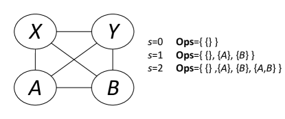
Figure 2: An example CPDAG ${\cal C}$ and the resulting operators generated by Selective-Generate-Ops(${\cal C}$,$X$,$Y$,$s$) for various values of $s$.

5 EXPERIMENTS

In this section, we present a simple synthetic experiment comparing SBES and BES that demonstrates the value of pruning operators. In our experiment we used an oracle scoring function. In particular, given a generative model ${\cal G}$, our scoring function computes the minimum-description-length score assuming a data size of five billion records, but without actually sampling any data: instead, we use exact inference in ${\cal G}$ (i.e., instead of counting from data) to compute the conditional probabilities needed to compute the expected log loss. This allows us to get near-asymptotic behavior without the need to sample data. To evaluate the cost of running each algorithm, we counted the number of times the scoring function was called on a unique node and parent-set combination; we cached these scores away so that if they were needed multiple times during a run of the algorithm, they were only computed (and counted) once.

In Figure 3, we show the average number of scoring-function calls required to complete BES and SBES when starting from a complete graph over a domain of $n$ binary variables, for varying values of $n$. Each average is taken over ten trials, corresponding to ten random generative models. All variables in the domain were binary. We generated the structure of each generative model as follows. First, we enumerated all node pairs by randomly permuting the nodes and taking each node in turn with all of its predecessors in turn. For each node pair in turn, we chose to attempt an edge insertion with probability one half. For each attempt, we added an edge if doing so (1) did not create a cycle and (2) did not result in a node having more than two parents; if an edge could be added in either direction, we chose the direction at random. We sampled the conditional distributions for each node and each parent configuration from a uniform Dirichlet distribution with equivalent-sample size of one. We ran SBES with $\Pi_{PS}^{2}$.

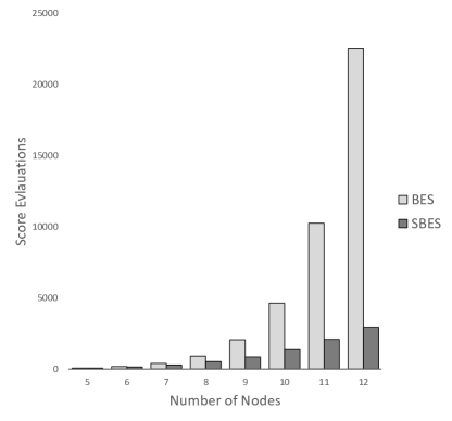
Figure 3: Number of score evaluations needed to run BES and SBES, starting from the complete graph, for a range of domain sizes.

Our results show clearly the exponential dependence of BES on the number of nodes in the clique, and the increasing savings we get with SBES, leveraging the fact that $\Pi_{PS}^{2}$ holds in the generative structure.

Note that to realize large savings in practice, when GES runs FES instead of starting from a dense graph, a (relatively sparse) generative distribution must lead FES to an equivalence class containing a (relatively dense) undirected clique that is subsequently “thinned” during BES. We can synthesize challenging grid distributions to force FES into such states, but it is not clear how realistic such distributions are in practice. When we re-run the clique experiment above, but where we instead start both BES and SBES from the model that results from running FES (i.e., with no polynomial-time guarantee), the savings from SBES are small due to the fact that the subsequent equivalence classes do not contain large cliques.

6 CONCLUSION

Through our selective greedy equivalence search algorithm SGES, we have demonstrated how to leverage graph-theoretic properties to reduce the need to score graphs during score-based search over equivalence classes of Bayesian networks. Furthermore, we have shown that for graph-theoretic complexity properties including maximum-clique size, maximum number of parents, and v-width, we can guarantee that the number of score evaluations is polynomial in the number of nodes and exponential in these complexity measures.

The fact that we can use our approach to selectively choose operators for any hereditary and equivalence invariant graph-theoretic property provides the opportunity to explore alternative complexity measures. Another candidate complexity measure is the maximum number of v-structures. Although the corresponding property does not limit the maximum size of a clique in ${\bf H}$, it limits directly the size $|\mbox{${\bf H}$}|$ for every operator. Thus it would be easy to enumerate these operators efficiently. Another complexity measure of interest is treewidth, due to the fact that exact inference in a Bayesian-network model is takes time exponential in this measure.

The results we have presented are for the general Bayesian-network learning problem. It is interesting to consider the implications of our results for the problem of learning particular subsets of Bayesian networks. One natural class that we discussed in Section 2 is that of polytrees. If we assume that the generative distribution is perfect with respect to a polytree then we know the v-width of the generative graph is one. This implies, in the limit of large data, that we can recover the structure of the generative graph with a polynomial number of score evaluations. This provides a score-based recovery algorithm analogous to the constraint-based approach of Geiger et al. (1990).

We presented a simple complexity analysis for the purpose of demonstrating that SGES uses a only polynomial number of calls to the scoring function. We leave as future work a more careful analysis that establishes useful constants in this polynomial. In particular, we can derive tighter bounds on the total number of node-and-parent-configurations that are needed to score all the operators for each CPDAG, and by caching these configuration scores we can further take advantage of the fact that most operators remain valid (i.e., the preconditions still hold) and have the same score after each transformation.

Finally, we plan to investigate practical implementations of poly-FES that have the polynomial-time guarantees needed for SGES.

Appendices

In the following two appendices, we prove Theorem 2.

Appendix A Additional Background

In this section, we introduce additional background material needed for the proofs.

A.1 Additional Notation

To express sets of variables more compactly, we often use a comma to denote set union (e.g., we write $\mbox{${\bf X}$}=\mbox{${\bf Y}$},\mbox{${\bf Z}$}$ as a more compact version of $\mbox{${\bf X}$}=\mbox{${\bf Y}$}\cup\mbox{${\bf Z}$}$). We also will sometimes remove the comma (e.g., ${\bf Y}$${\bf Z}$). When a set consists of a singleton variable, we often use the variable name as shorthand for the set containing that variable (e.g., we write $\mbox{${\bf X}$}=\mbox{${\bf Y}$}\setminus Z$ as shorthand for $\mbox{${\bf X}$}=\mbox{${\bf Y}$}\setminus\{Z\}$).

We say a node $N$ is a descendant of $Y$ if $N=Y$ or there is a directed path from $Y$ to $N$. We use ${\cal H}$-descendant to refer to a descendant in a particular DAG ${\cal H}$. We say a node $N$ is a proper descendant of $Y$ if $N$ is a descendant of $Y$ and $N\not=Y$. We use ${\bf NonDe}^{{\cal H}}_{Y}$ to denote the non-descendants of node $Y$ in ${\cal G}$. We use ${\bf Pa}^{{\cal H}}_{Y\downarrow X_{1}X_{2}\ldots X_{n}}$ as shorthand for $\mbox{${\bf Pa}^{{\cal H}}_{Y}$}\setminus\{X_{1},\ldots,X_{n}\}$. For example, to denote all the parents of $Z$ in ${\cal H}$ except for $X$ and $Y$, we use ${\bf Pa}^{{\cal H}}_{Z\downarrow XY}$.

A.2 D-separation and Acvite Paths

The independence constraints implied by a DAG structure are characterized by the d-separation criterion. Two nodes $A$ and $B$ are said to be d-separated in a DAG ${\cal G}$ given a set of nodes ${\bf S}$ if and only if there is no active path in ${\cal G}$ between $A$ and $B$ given ${\bf S}$. The standard definition of an active path is a simple path for which each node $W$ along the path either (1) has converging arrows (i.e., $\rightarrow W\leftarrow$) and $W$ or a descendant of $W$ is in ${\bf S}$ or (2) does not have converging arrows and $W$ is not in ${\bf S}$. By simple, we mean that the path never passes through the same node twice.

To simplify our proofs, we use an equivalent definition of an active path—that need not be simple—where each node $W$ along the path either (1) has converging arrows and $W$ is in ${\bf S}$ or (2) does not have converging arrows and $W$ is not in ${\bf S}$. In other words, instead of allowing a segment $\rightarrow W\leftarrow$ to be included in a path by virtue of a descendant of $W$ belonging to ${\bf S}$, we require that the path include the sequence of edges from $W$ to that descendant and then back again. For those readers familiar with the celebrated “Bayes ball” algorithm of Shachter (1998) for testing d-separation, our expanded definition of an active path is simply a valid path that the ball can take between $A$ and $B$.

We use $\mbox{${\bf X}$}\mbox{$\perp\!\!\perp$}_{{\cal G}}\mbox{${\bf Y}$}|\mbox{${\bf Z}$}$ to denote the assertion that DAG ${\cal G}$ imposes the constraint that variables ${\bf X}$ are independent of variables ${\bf Y}$ given variables ${\bf Z}$.When a node $W$ along a path has converging arrows, we say that $W$ is a collider at that position in the path.

The direction of each terminal edge in an active path—that is, the first and last edge encountered in a traversal from one end of the path to the other—is important for determining whether we can append two active paths together to make a third active path. We say that a path $\pi(A,B)$ is into $A$ if the terminal edge incident to $A$ is oriented toward $A$ (i.e., $A\leftarrow$). Similarly, the path is into $B$ if the terminal edge incident to $B$ is oriented toward $B$. If a path is not into an endpoint $A$, we say that the path is out of $A$. Using the following result from Chickering (2002), we can combine active paths together.

Lemma 1.

(Chickering, 2002) Let $\pi(A,B)$ be an ${\bf S}$-active path between $A$ and $B$, and let $\pi(B,C)$ be an ${\bf S}$-active path between $B$ and $C$. If either path is out of $B$, then the concatenation of $\pi(A,B)$ and $\pi(B,C)$ is an ${\bf S}$-active path between $A$ and $C$.

Given a DAG ${\cal H}$ that is an IMAP of DAG ${\cal G}$, we use the d-separation criterion in two general ways in our proofs. First, we identify d-separation facts that hold in ${\cal H}$ and conclude that they must also hold in ${\cal G}$. Second, we identify active paths in ${\cal G}$ and conclude that there must be corresponding active paths in ${\cal H}$.

A.3 Independence Axioms

In many of our proofs, we would like to reason about the independence facts that hold in DAG ${\cal G}$ without knowing what its structure is, which makes using the d-separation criterion problematic. As described in Pearl (1988), any set of independence facts characterized by the d-separation criterion also respect the independence axioms shown in Figure 4. These axioms allow us to take a set of independence facts in some unknown ${\cal G}$ (e.g., that are implied by d-separation in ${\cal H}$), and derive new independence facts that we know must also hold in ${\cal G}$.

Symmetry:	$\mbox{${\bf X}$}\mbox{$\perp\!\!\perp$}\mbox{${\bf Y}$}|\mbox{${\bf Z}$}$	$\Longleftrightarrow$	$\mbox{${\bf Y}$}\mbox{$\perp\!\!\perp$}\mbox{${\bf X}$}|\mbox{${\bf Z}$}$
Decomposition:	$\mbox{${\bf X}$}\mbox{$\perp\!\!\perp$}\mbox{${\bf Y}$},\mbox{${\bf W}$}|\mbox{${\bf Z}$}$	$\Longrightarrow$	$\mbox{${\bf X}$}\mbox{$\perp\!\!\perp$}\mbox{${\bf Y}$}|\mbox{${\bf Z}$}$  +   $\mbox{${\bf X}$}\mbox{$\perp\!\!\perp$}\mbox{${\bf W}$}|\mbox{${\bf Z}$}$
Composition:	$\mbox{${\bf X}$}\mbox{$\perp\!\!\perp$}\mbox{${\bf Y}$}|\mbox{${\bf Z}$}$  +   $\mbox{${\bf X}$}\mbox{$\perp\!\!\perp$}\mbox{${\bf W}$}|\mbox{${\bf Z}$}$	$\Longrightarrow$	$\mbox{${\bf X}$}\mbox{$\perp\!\!\perp$}\mbox{${\bf Y}$},\mbox{${\bf W}$}|\mbox{${\bf Z}$}$
Intersection:	$\mbox{${\bf X}$}\mbox{$\perp\!\!\perp$}\mbox{${\bf Y}$}|\mbox{${\bf Z}$},\mbox{${\bf W}$}$  +   $\mbox{${\bf X}$}\mbox{$\perp\!\!\perp$}\mbox{${\bf W}$}|\mbox{${\bf Z}$},\mbox{${\bf Y}$}$	$\Longrightarrow$	$\mbox{${\bf X}$}\mbox{$\perp\!\!\perp$}\mbox{${\bf Y}$},\mbox{${\bf W}$}|\mbox{${\bf Z}$}$
Weak Union:	$\mbox{${\bf X}$}\mbox{$\perp\!\!\perp$}\mbox{${\bf Y}$},\mbox{${\bf W}$}|\mbox{${\bf Z}$}$	$\Longrightarrow$	$\mbox{${\bf X}$}\mbox{$\perp\!\!\perp$}\mbox{${\bf Y}$}|\mbox{${\bf Z}$},\mbox{${\bf W}$}$
Contraction:	$\mbox{${\bf X}$}\mbox{$\perp\!\!\perp$}\mbox{${\bf W}$}|\mbox{${\bf Z}$},\mbox{${\bf Y}$}$  +   $\mbox{${\bf X}$}\mbox{$\perp\!\!\perp$}\mbox{${\bf Y}$}|\mbox{${\bf Z}$}$	$\Longleftarrow$	$\mbox{${\bf X}$}\mbox{$\perp\!\!\perp$}\mbox{${\bf Y}$},\mbox{${\bf W}$}|\mbox{${\bf Z}$}$
Weak Transitivity:	$\mbox{${\bf X}$}\mbox{$\perp\!\!\perp$}\mbox{${\bf Y}$}|\mbox{${\bf Z}$}$  +   $\mbox{${\bf X}$}\mbox{$\perp\!\!\perp$}\mbox{${\bf Y}$}|\mbox{${\bf Z}$},T$	$\Longrightarrow$	$\mbox{${\bf X}$}\mbox{$\perp\!\!\perp$}T|\mbox{${\bf Z}$}$  OR   $\mbox{${\bf Y}$}\mbox{$\perp\!\!\perp$}T|\mbox{${\bf Z}$}$

Figure 4: The DAG-perfect independence axioms.

Throughout the proofs, we will often use the Symmetry axiom implicitly. For example, if we have $A\mbox{$\perp\!\!\perp$}B,C|D$ we might claim that $B\mbox{$\perp\!\!\perp$}A|C,D$ follows from Weak Union, as opposed to concluding $A\mbox{$\perp\!\!\perp$}B|C,D$ from Weak Union and then applying Symmetry. We will frequently identify independence constraints in ${\cal H}$ and conclude that they hold in ${\cal G}$, without explicitly justifying this with because ${\cal G}\leq{\cal H}$. For example, we will say:

Because $A$ is a non-descendant of $B$ in ${\cal H}$, it follows from the Markov conditions that $A\mbox{$\perp\!\!\perp$}_{\mbox{${\cal G}$}}B|\mbox{${\bf Pa}^{{\cal H}}_{B}$}$.

In other words, to be explicit we would say that $A\mbox{$\perp\!\!\perp$}_{\mbox{${\cal H}$}}B|\mbox{${\bf Pa}^{{\cal H}}_{B}$}$ follows from the Markov conditions, and the independence holds in ${\cal G}$ because ${\cal G}\leq{\cal H}$.

The Composition axiom states that if ${\bf X}$ is independent of both ${\bf Y}$ and ${\bf W}$ individually given ${\bf Z}$, then ${\bf X}$ is independent of them jointly. If we have more than two such sets that are independent of ${\bf X}$, we can apply the Composition axiom repeatedly to combine them all together. To simplify, we will do this combination implicitly, and assume that the Composition axiom is defined more generally. Thus, for example, we might have:

Because $X\mbox{$\perp\!\!\perp$}Y|\mbox{${\bf Z}$}$ for every $Y\in\mbox{${\bf Y}$}$, we conclude by the Composition axiom that $X\mbox{$\perp\!\!\perp$}\mbox{${\bf Y}$}|\mbox{${\bf Z}$}$.

Appendix B Proofs

In this section, we provide a number of intermediate results that lead to a proof of Theorem 2.

B.1 Intermediate Result: “The Deletion Lemma”

Given DAGs ${\cal G}$ and ${\cal H}$ for which ${\cal G}<{\cal H}$, we say that an edge $e$ from ${\cal H}$ is deletable in ${\cal H}$ with respect to ${\cal G}$ if, for the DAG ${\cal H}^{\prime}$ that results after removing $e$ from ${\cal H}$, we have ${\cal G}\leq{\cal H}$. We will say that an edge is deletable in ${\cal H}$ or simply deletable if ${\cal G}$ or both DAGs, respectively, are clear from context. The following lemma establishes necessary and sufficient conditions for an edge to be deletable.

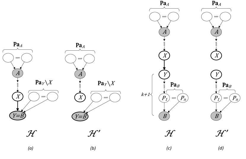
Figure 5: Relevant portions of ${\cal H}$ and ${\cal H}^{\prime}$ for the inductive proof of Lemma 2: (a) and (b) are for the basis and (c) and (d) are for the induction hypothesis.

Lemma 2.

Let ${\cal G}$ and ${\cal H}$ be two DAGs such that ${\cal G}\leq{\cal H}$. An edge $X\rightarrow Y$ is deletable in ${\cal H}$ with respect to ${\cal G}$ if and only if $Y\mbox{$\perp\!\!\perp$}_{{\cal G}}X|\mbox{${\bf Pa}^{{\cal H}}_{Y}$}\setminus X$.

Proof: Let ${\cal H}^{\prime}$ be the DAG resulting from removing the edge. The “only if” follows immediately because the given independence is implied by ${\cal H}^{\prime}$. For the “if”, we show that for every node $A$ and every node $B\in\mbox{${\bf NonDe}^{{\cal H}^{\prime}}_{A}$}$, the independence $A\mbox{$\perp\!\!\perp$}_{{\cal G}}B|\mbox{${\bf Pa}^{{\cal H}^{\prime}}_{A}$}$ holds (in ${\cal G}$). We need only consider $(A,B)$ pairs for which $B$ is a descendant in ${\cal H}$ but not in ${\cal H}^{\prime}$; if the “descendant” relationship has not changed, we know the independence holds by virtue of ${\cal G}\leq{\cal H}$ and the fact that deleting an edge results in strictly more independence constraints.

The proof follows by induction on the length of the longest directed path in ${\cal H}^{\prime}$ from $Y$ to $B$. For the base case (see Figure 5a and Figure 5b), we start with a longest path of length zero; in other words, $B=Y$. Because $A$ is an ancestor of $Y$ in ${\cal H}$, both it and its parents must be non-descendants of $Y$ in ${\cal H}$, and therefore the Markov conditions in ${\cal H}$ imply

$$Y\mbox{$\perp\!\!\perp$}_{{\cal G}}A,\mbox{${\bf Pa}^{{\cal H}}_{A}$}|\mbox{${\bf Pa}^{{\cal H}}_{Y}$}$$ (2)

Given the independence fact assumed in the lemma, we can apply the Contraction axiom to remove $X$ from the conditioning set in (2), and then apply the Weak Union axiom to move ${\bf Pa}^{{\cal H}}_{A}$ into the conditioning set to conclude

$$Y\mbox{$\perp\!\!\perp$}_{{\cal G}}A|\mbox{${\bf Pa}^{{\cal H}}_{Y}$}\setminus X,\mbox{${\bf Pa}^{{\cal H}}_{A}$}$$ (3)

Neither $Y$ nor its new parents $\mbox{${\bf Pa}^{{\cal H}}_{Y}$}\setminus X$ can be descendants of $A$ in ${\cal H}^{\prime}$, else $B$ would remain a descendant of $A$ after the deletion, and thus we conclude by the Markov conditions in ${\cal H}$ that

$$A\mbox{$\perp\!\!\perp$}_{{\cal G}}\mbox{${\bf Pa}^{{\cal H}}_{Y}$}\setminus X|\mbox{${\bf Pa}^{{\cal H}}_{A}$}$$ (4)

Applying the Contraction axiom to (3) and (4), we have

$$A\mbox{$\perp\!\!\perp$}_{{\cal G}}Y|\mbox{${\bf Pa}^{{\cal H}}_{A}$}$$

and because $\mbox{${\bf Pa}^{{\cal H}^{\prime}}_{A}$}=\mbox{${\bf Pa}^{{\cal H}}_{A}$}$ the lemma follows.

For the induction step (see Figure 5c and Figure 5d), we assume the lemma holds for all nodes whose longest path from $Y$ is $\leq k$, and we consider a $B$ for which the longest path from $Y$ is $k+1$. Consider any parent $P$ of node $B$. If $P$ is a descendant of $Y$, the longest path from $Y$ to $B$ must be $\leq k$, else we have a path to $B$ that is longer than $k+1$. If $P$ is not a descendant of $Y$, then $P$ is also not a descendant of $A$ in ${\cal H}$, else $B$ would be a descendant of $A$ in ${\cal H}^{\prime}$. Thus, for every parent $P$, we conclude

$$A\mbox{$\perp\!\!\perp$}_{{\cal G}}P|\mbox{${\bf Pa}^{{\cal H}}_{A}$}$$

either by the induction hypothesis or by the fact that $P$ is a non-descendant of $A$ in ${\cal H}$. From the Composition axiom we can combine these individual parents together, yielding

$$A\mbox{$\perp\!\!\perp$}_{{\cal G}}\mbox{${\bf Pa}^{{\cal H}}_{B}$}|\mbox{${\bf Pa}^{{\cal H}}_{A}$}$$ (5)

Because $B$ is a descendant of $A$ in ${\cal H}$, we know that $A$ and all of its parents ${\bf Pa}^{{\cal H}}_{A}$ are non-descendants of $B$ in ${\cal H}$, and thus

$$B\mbox{$\perp\!\!\perp$}_{{\cal G}}A,\mbox{${\bf Pa}^{{\cal H}}_{A}$}|\mbox{${\bf Pa}^{{\cal H}}_{B}$}$$ (6)

Applying the Weak Union axiom to (6) yields

$$B\mbox{$\perp\!\!\perp$}_{{\cal G}}A|\mbox{${\bf Pa}^{{\cal H}}_{A}$},\mbox{${\bf Pa}^{{\cal H}}_{B}$}$$ (7)

and finally applying the Contraction axiom to (5) and (7) yields

$$A\mbox{$\perp\!\!\perp$}_{{\cal G}}B|\mbox{${\bf Pa}^{{\cal H}}_{A}$}$$

Because the parents of $A$ are the same in both ${\cal H}$ and ${\cal H}^{\prime}$, the lemma follows. ∎

B.2 Intermediate Result: “The Deletion Theorem”

We define the pruned variables for ${\cal G}$ and ${\cal H}$—denoted ${\bf Prune}({\cal G},{\cal H})$– to be the subset of the variables that remain after we repeatedly remove from both graphs any common sink nodes (i.e., nodes with no children) with the same parents in both graphs. For $\mbox{${\bf V}$}=\mbox{${\bf Prune}({\cal G},{\cal H})$}$, let ${\overline{\mbox{${\bf V}$}}}$ denote the complement of ${\bf V}$. Note that every node in ${\overline{\mbox{${\bf V}$}}}$ has the same parents and children in both ${\cal G}$ and ${\cal H}$, and that $\mbox{${\cal G}[\overline{\mbox{${\bf V}$}}]$}=\mbox{${\cal H}[\overline{\mbox{${\bf V}$}}]$}$.

We use ${\cal G}$-leaf   to denote any node in ${\cal G}$ that has no children. For any ${\cal G}$-leaf   $L$, we say that $L$ is an ${\cal H}$-lowest ${\cal G}$-leaf   if no proper descendant of $L$ in ${\cal H}$ is a ${\cal G}$-leaf  . Note that we are discussing two DAGs in this case: $L$ is a leaf in ${\cal G}$, and out of all nodes that are leaves in ${\cal G}$, $L$ is the one that is lowest in the other DAG ${\cal H}$. To avoid ambiguity, we often prefix other common graph concepts (e.g., ${\cal G}$-child and ${\cal H}$-parent) to emphasize the specific DAG to which we are referring.

We need the following result from Chickering (2002).

Lemma 3.

(Chickering, 2002) Let ${\cal G}$ and ${\cal H}$ be two DAGs containing a node $Y$ that is a sink in both DAGs and for which $\mbox{${\bf Pa}^{{\cal G}}_{Y}$}=\mbox{${\bf Pa}^{{\cal H}}_{Y}$}$. Let ${\cal G}^{\prime}$ and ${\cal H}^{\prime}$ denote the subgraphs of ${\cal G}$ and ${\cal H}$, respectively, that result by removing node $Y$ and all its in-coming edges. Then ${\cal G}\leq{\cal H}$ if and only if ${\cal G}^{\prime}\leq{\cal H}^{\prime}$.

By repeatedly applying Lemma 3, the following corollary follows immediately.

Corollary 1.

Let $\mbox{${\bf V}$}=\mbox{${\bf Prune}({\cal G},{\cal H})$}$. Then ${\cal G}\leq{\cal H}$ if and only if ${\cal G}_{\mbox{${\bf V}$}}\leq{\cal H}_{\mbox{${\bf V}$}}$.

We now present the “deletion theorem”, which is the basis for Theorem 2.

Theorem 4.

Let ${\cal G}$ and ${\cal H}$ be DAGs for which ${\cal G}\leq{\cal H}$, let $\mbox{${\bf V}$}=\mbox{${\bf Prune}({\cal G},{\cal H})$}$, and let $L$ be any ${\cal H}[\mbox{${\bf V}$}]$-lowest ${\cal G}[\mbox{${\bf V}$}]$-leaf. Then,

1. If $L$ does not have any ${\cal H}[\mbox{${\bf V}$}]$-children, then for every $D\in\mbox{${\bf V}$}$ that is an ${\cal H}[\mbox{${\bf V}$}]$-parent of $L$ but not a ${\cal G}[\mbox{${\bf V}$}]$-parent of $L$, $D\rightarrow L$ is deletable in ${\cal H}$.

2. If $L$ has at least one ${\cal H}[\mbox{${\bf V}$}]$-child, let $A$ be any ${\cal H}[\mbox{${\bf V}$}]$-highest child; one of the following three properties must hold in ${\cal H}$:

   1. $L\rightarrow A$ is covered.

   2. There exists an edge $A\leftarrow B$, where $L$ and $B$ are not adjacent, and either $L\rightarrow A$ or $A\leftarrow B$ (or both) are deletable.

   3. There exists an edge $D\rightarrow L$, where $D$ and $A$ are not adjacent, and either $D\rightarrow L$ or $L\rightarrow A$ (or both) are deletable.

Proof: As a consequence of Corollary 1, the lemma holds if and only if it holds for any graphs ${\cal G}$ and ${\cal H}$ for which there are no nodes that are sinks in both graphs with the same parents; in other words, ${\cal G}={\cal G}_{\mbox{${\bf V}$}}$ and ${\cal H}={\cal H}_{\mbox{${\bf V}$}}$. Thus, to vastly simplify the notation for the remainder of the proof, we will assume that this is the case, and therefore $L$ is a leaf node in ${\cal G}$, $A$ is a highest child of $L$ in ${\cal H}$, and the restriction of $B$ and $D$ to ${\bf V}$ is vacuous.

For case (1), we know that $\mbox{${\bf Pa}^{{\cal G}}_{L}$}\subseteq\mbox{${\bf Pa}^{{\cal H}}_{L}$}$, else there would be some edge in $X\rightarrow L$ in ${\cal G}$ for which $X$ and $L$ are not adjacent in ${\cal H}$, contradicting ${\cal G}\leq{\cal H}$. Because $L$ is a leaf in ${\cal G}$, all non-parents must also be non-descendants, and hence $L\mbox{$\perp\!\!\perp$}_{{\cal G}}X|\mbox{${\bf Pa}^{{\cal G}}_{L}$}$ for all $X$. It follows that for every $D\in\{\mbox{${\bf Pa}^{{\cal H}}_{L}$}\setminus\mbox{${\bf Pa}^{{\cal G}}_{L}$}\}$, $D\rightarrow Y$ is deletable in ${\cal H}$. There must exist such a $D$, else $L$ would be in $\mbox{${\bf V}$}=\mbox{${\bf Prune}({\cal G},{\cal H})$}$.

For case (2), we now show that at least one of the properties must hold. Assume that the first property does not hold, and demonstrate that one of the other two properties must hold. If the first property does not hold then we know that in ${\cal H}$ either there exists an edge $A\leftarrow B$ where $B$ is not a parent of $L$, or there exists an edge $D\rightarrow L$ where $D$ is not a parent of $A$. Thus the pre-conditions of at least one of the remaining two properties must hold.

Suppose ${\cal H}$ contains the edge $A\leftarrow B$ where $B$ is not a parent of $L$. Then we conclude immediately from Corollary 2 that either $L\rightarrow A$ or $A\leftarrow B$ is deletable in ${\cal H}$.

Suppose ${\cal H}$ contains the edge $D\rightarrow L$ where $D$ is not a parent of $A$. Then the set ${\bf D}$ containing all parents of $L$ that are not parents of $A$ is non-empty. Let $\mbox{${\bf R}$}=\mbox{${\bf Pa}^{{\cal H}}_{A}$}\cap\mbox{${\bf Pa}^{{\cal H}}_{L}$}$ be the shared parents of $L$ and $A$, and let $\mbox{${\bf T}$}=\mbox{${\bf Pa}^{{\cal H}}_{A\downarrow\mbox{${\bf R}$}L}$}$ be the remaining non-$L$ parents of $A$ in ${\cal H}$, so that we have $\mbox{${\bf Pa}^{{\cal H}}_{A}$}=L,\mbox{${\bf R}$},\mbox{${\bf T}$}$ and $\mbox{${\bf Pa}^{{\cal H}}_{L}$}=\mbox{${\bf R}$},\mbox{${\bf D}$}$. Because no node in ${\bf D}$ is a child or a descendant of $A$, lest ${\cal H}$ contains a cycle, we know that ${\cal H}$ contains the following independence constraint that must hold in ${\cal G}$:

$$A\mbox{$\perp\!\!\perp$}_{{\cal G}}\mbox{${\bf D}$}|L,\mbox{${\bf R}$},\mbox{${\bf T}$}$$ (8)

Because $L$ is a leaf node in ${\cal G}$, it is impossible to create a new active path by removing it from the conditioning set, and hence we also know

$$A\mbox{$\perp\!\!\perp$}_{{\cal G}}\mbox{${\bf D}$}|\mbox{${\bf R}$},\mbox{${\bf T}$}$$ (9)

Applying the Weak Transitivity axiom to Independence 8 and Independence 9, we conclude either $A\mbox{$\perp\!\!\perp$}_{{\cal G}}L|\mbox{${\bf R}$},\mbox{${\bf T}$}$—in which case $L\rightarrow A$ is deletable–or

$$L\mbox{$\perp\!\!\perp$}_{{\cal G}}\mbox{${\bf D}$}|\mbox{${\bf R}$},\mbox{${\bf T}$}$$ (10)

We know that no node in ${\bf T}$ can be a descendant of $L$, or else $A$ would not be the highest child of $L$. Thus, because $L$ is independent of any non-descendants given its parents we have

$$L\mbox{$\perp\!\!\perp$}_{{\cal G}}\mbox{${\bf T}$}|\mbox{${\bf R}$},\mbox{${\bf D}$}$$ (11)

Applying the Intersection axiom to Independence 10 and Independence 11, we have

$$L\mbox{$\perp\!\!\perp$}_{{\cal G}}\mbox{${\bf D}$}|\mbox{${\bf R}$}$$ (12)

In other words, $L$ is independent of all of the nodes in ${\bf D}$ given the other parents. By applying the Weak Union axiom, we can pull all but one of the nodes in ${\bf D}$ into the conditioning set to obtain

$$L\mbox{$\perp\!\!\perp$}_{{\cal G}}D|\mbox{${\bf R}$},\{\mbox{${\bf D}$}\setminus D\}$$ (13)

and hence $D\rightarrow L$ is deletable for each such $D$. ∎

B.3 Intermediate Result: “Add A Singleton Descendant to the Conditioning Set”

The intuition behind the following lemma is that if $L$ is an ${\cal H}$-lowest ${\cal G}$-leaf  , no v-structure below $L$ in ${\cal H}$ can be “real” in terms of the dependences in ${\cal G}$: for any $Y$ below $L$ that is independent of some other node $X$, they remain independent when we condition on any singleton descendant $Z$ of $Y$, even if $Z$ is also a descendant of $X$. The lemma is stated in a somewhat complicated manner because we want to use it both when (1) $X$ and $Y$ are adjacent but the edge is known to be deletable and (2) $X$ and $Y$ are not adjacent. We also find it convenient to include, in addition to $Y$’s non-$X$ parents, an arbitrary additional set of non-descendants ${\bf S}$.

Lemma 4.

Let $Y$ be any ${\cal H}$-descendant of an ${\cal H}$-lowest ${\cal G}$-leaf  . If

$$Y\mbox{$\perp\!\!\perp$}_{\mbox{${\cal G}$}}X|\mbox{${\bf Pa}^{{\cal H}}_{Y\downarrow X}$},\mbox{${\bf S}$}$$

for $\{X,\mbox{${\bf S}$}\}\subseteq\mbox{${\bf NonDe}^{{\cal H}}_{Y}$}$, then $Y\mbox{$\perp\!\!\perp$}_{{\cal G}}X|\mbox{${\bf Pa}^{{\cal H}}_{Y\downarrow X}$},\mbox{${\bf S}$},Z$ for any proper ${\cal H}$-descendant $Z$ of $Y$.

Proof: To simplify notation, let $\mbox{${\bf R}$}=\mbox{${\bf Pa}^{{\cal H}}_{Y\downarrow X}$},\mbox{${\bf S}$}$. Assume the lemma does not hold and thus $Y\mbox{$\not\!\!\!\mbox{$\perp\!\!\perp$}$}_{{\cal G}}X|\mbox{${\bf R}$},Z$. Consider any $(\mbox{${\bf R}$},Z)$-active path $\pi_{XY}$ between $X$ and $Y$ in ${\cal G}$. Because $Y\mbox{$\perp\!\!\perp$}_{{\cal G}}X|\mbox{${\bf R}$}$, this path cannot be active without $Z$ in the conditioning set, which means that $Z$ must be on the path, and it must be a collider in every position it occurs. Without loss of generality, assume $Z$ occurs exactly once as a collider along the path (we can simply delete the sub-path between the first and last occurrence of $Z$, and the resulting path will remain active), and let $\pi_{XZ}$ be the sub-path from $X$ to $Z$ along $\pi_{XY}$, and let $\pi_{ZY}$ be the sub-path from $Z$ to $Y$ along $\pi_{XY}$.

Because $Z$ is a proper descendant of $Y$ in ${\cal H}$, and $Y$ is a descendant of an ${\cal H}$-lowest ${\cal G}$-leaf  , we know $Z$ cannot be a ${\cal G}$-leaf  , else it would be lower than $L$ in ${\cal H}$. That means that in ${\cal G}$, there is a directed path $\pi_{ZL^{\prime}}=Z\rightarrow\ldots\rightarrow L^{\prime}$ consisting of at least one edge from $Z$ to some ${\cal G}$-leaf  . No node $T$ along this path can be in ${\bf R}$, else we could splice in the path $Z\rightarrow\ldots\rightarrow T\leftarrow\ldots\leftarrow Z$ between $\pi_{XZ}$ and $\pi_{ZY}$, and the resulting path would remain active without $Z$ in the conditioning set. Note that this means that $L^{\prime}$ cannot belong to $\mbox{${\bf Pa}^{{\cal H}}_{Y\downarrow X}$}\subseteq\mbox{${\bf R}$}$. Similarly, the path cannot reach $X$ or $Y$, else we could combine this out-of-$Z$ path with $\pi_{ZY}$ or $\pi_{XZ}$, respectively, to again find an ${\bf R}$-active path between $X$ and $Y$. We know that in ${\cal H}$, $L^{\prime}$ must be a non-descendant of $Y$, else $L^{\prime}$ would be a lower ${\cal G}$-leaf   than $L$ in ${\cal H}$. Because $X\cup\mbox{${\bf R}$}$ contains all of $Y$’s parents and none of its descendants, and because (as we noted) $L^{\prime}$ cannot be in $X\cup\mbox{${\bf R}$}$, we know ${\cal H}$ contains the independence $Y\mbox{$\perp\!\!\perp$}_{{\cal H}}L^{\prime}|X,\mbox{${\bf R}$}$. But we just argued that the (directed) path $\pi_{ZL^{\prime}}$ in ${\cal G}$ does not pass through any of $X,Y,\mbox{${\bf R}$}$, which means that it constitutes an out-of $Z$ $(\mbox{${\bf R}$},X)$-active path that can be combined with $\pi_{ZY}$ to produce a $(\mbox{${\bf R}$},X)$-active path between $Z$ and $L^{\prime}$, yielding a contradiction. ∎

B.4 Intermediate Result: The “Weak-Transitivity Deletion” Lemma

The next lemma considers a collider $X\rightarrow Z\leftarrow Y$ in ${\cal H}$ where either there is no edge between $X$ and $Y$ (i.e., the collider is a v-structure) or the edge is deletable. The lemma states that if $X$ and $Y$ remain independent when conditioning on their common child—where all the non-$\{X,Y,Z\}$ parents of all three nodes are also in the conditioning set—then one of the two edges must be deletable.

Lemma 5.

Let $X\rightarrow Z$ and $Y\rightarrow Z$ be two edges in ${\cal H}$. If $X\mbox{$\perp\!\!\perp$}_{{\cal G}}Y|\mbox{${\bf Pa}^{{\cal H}}_{X\downarrow Y}$},\mbox{${\bf Pa}^{{\cal H}}_{Y\downarrow X}$},\mbox{${\bf Pa}^{{\cal H}}_{Z\downarrow XY}$}$ and $X\mbox{$\perp\!\!\perp$}_{{\cal G}}Y|\mbox{${\bf Pa}^{{\cal H}}_{X\downarrow Y}$},\mbox{${\bf Pa}^{{\cal H}}_{Y\downarrow X}$},\mbox{${\bf Pa}^{{\cal H}}_{Z\downarrow XY}$},Z$ (i.e., $Z$ added to the conditioning set), then at least one of the following must hold: $Z\mbox{$\perp\!\!\perp$}_{{\cal G}}X|\mbox{${\bf Pa}^{{\cal H}}_{Z\downarrow X}$}$ or $Z\mbox{$\perp\!\!\perp$}_{{\cal G}}Y|\mbox{${\bf Pa}^{{\cal H}}_{Z\downarrow Y}$}$.

Proof: Let $\mbox{${\bf S}$}=\{\mbox{${\bf Pa}^{{\cal H}}_{X\downarrow Y}$},\mbox{${\bf Pa}^{{\cal H}}_{Y\downarrow X}$}\}\setminus\mbox{${\bf Pa}^{{\cal H}}_{Z\downarrow XY}$}$ be the (non-$X$ and non-$Y$) parents of $X$ and $Y$ that are not parents of $Z$, and let $\mbox{${\bf R}$}=\mbox{${\bf Pa}^{{\cal H}}_{Z\downarrow XY}$}$ be all of $Z$’s parents other than $X$ and $Y$. Using this notation, we can re-write the two conditions of the lemma as:

$$X\mbox{$\perp\!\!\perp$}_{{\cal G}}Y|\mbox{${\bf R}$},\mbox{${\bf S}$}$$ (14)

and

$$X\mbox{$\perp\!\!\perp$}_{{\cal G}}Y|Z,\mbox{${\bf R}$},\mbox{${\bf S}$}$$ (15)

From the Weak Transitivity axiom we conclude from these two independences that either $Z\mbox{$\perp\!\!\perp$}_{{\cal G}}X|\mbox{${\bf R}$},\mbox{${\bf S}$}$ or $Z\mbox{$\perp\!\!\perp$}_{{\cal G}}X|\mbox{${\bf R}$},\mbox{${\bf S}$}$. Assume the first of these is true

$$Z\mbox{$\perp\!\!\perp$}_{{\cal G}}X|\mbox{${\bf R}$},\mbox{${\bf S}$}$$ (16)

If we apply the Composition axiom to the independences in Equation 14 and Equation 16 we get $X\mbox{$\perp\!\!\perp$}_{{\cal H}}Y,Z|\mbox{${\bf R}$},\mbox{${\bf S}$}$; applying the Weak Union axiom we can then pull $Y$ into the conditioning set to get:

$$Z\mbox{$\perp\!\!\perp$}_{{\cal H}}X|\{Y,\mbox{${\bf R}$}\},\mbox{${\bf S}$}$$ (17)

Because $\{Y,\mbox{${\bf R}$}\},X$ is precisely the parent set of $Z$, and because ${\bf S}$ (i.e., the parents of $Z$’s parents) cannot contain any descendant of $Z$, we know by the Markov conditions that

$$Z\mbox{$\perp\!\!\perp$}_{{\cal H}}\mbox{${\bf S}$}|\{Y,\mbox{${\bf R}$}\},X$$ (18)

Applying the Intersection Axiom to the independences in Equation 17 and Equation 18 yields:

$$Z\mbox{$\perp\!\!\perp$}_{{\cal H}}X|Y,\mbox{${\bf R}$}$$

Because $Y,\mbox{${\bf R}$}=\mbox{${\bf Pa}^{{\cal H}}_{Z\downarrow X}$}$, this means the first independence implied by the lemma follows.

If the second of the two independence facts that follow from Weak Transitivity hold (i.e., if $Z\mbox{$\perp\!\!\perp$}_{{\cal G}}X|\mbox{${\bf R}$},\mbox{${\bf S}$}$), then a completely parallel application of axioms leads to the second independence implied by the lemma. ∎

B.5 Intermediate Result: The “Move Lower” Lemma

Lemma 6.

Let $Y$ be any ${\cal H}$-descendant of an ${\cal H}$-lowest ${\cal G}$-leaf  . If there exists an $X\in\mbox{${\bf NonDe}^{{\cal H}}_{Y}$}$ that has a common ${\cal H}$-descendant with $Y$ and for which

$$Y\mbox{$\perp\!\!\perp$}_{{\cal G}}X|\mbox{${\bf Pa}^{{\cal H}}_{Y\downarrow X}$}$$

then there exists an edge $W\rightarrow Z$ that is deletable in ${\cal H}$, where $Z$ is a proper ${\cal H}$-descendant of $Y$.

Proof: Let $Z$ be the highest common descendant of $Y$ and $X$, let $D_{Y}$ be the lowest descendant of $Y$ that is a parent of $Z$, and let $D_{X}$ be any descendant of $X$ that is a parent of $Z$. We know that either (1) $D_{Y}=Y$ and $D_{X}=X$ or (2) $D_{Y}$ and $D_{X}$ are not adjacent and have no directed path connecting them; if this were not the case, and ${\cal H}$ contained a path $D_{Y}\rightarrow\ldots\rightarrow D_{X}$ ($D_{X}\rightarrow\ldots\rightarrow D_{Y}$) then $D_{X}$ ($D_{Y}$) would be a higher common descendant than $Z$. This means that in either case (1) or in case (2), we have

$$D_{Y}\mbox{$\perp\!\!\perp$}_{{\cal G}}D_{X}|\mbox{${\bf Pa}^{{\cal H}}_{D_{Y}\downarrow D_{X}}$}$$ (19)

For case (1), this is given to us explicitly in the statement of the lemma, and for case (2), $\mbox{${\bf Pa}^{{\cal H}}_{D_{Y}\downarrow D_{X}}$}=\mbox{${\bf Pa}^{{\cal H}}_{D_{Y}}$}$ and thus the independence holds from the Markov conditions in ${\cal H}$ because $D_{X}$ is a non-descendant of $D_{Y}$. Because in both cases we know there is no directed path from $D_{Y}$ to $D_{X}$, we know that all of ${\bf Pa}^{{\cal H}}_{D_{X}\downarrow D_{Y}}$ are non-descendants of $D_{Y}$, and thus we can add them (via Composition and Weak Union) to the conditioning set of Equation 19:

$$D_{Y}\mbox{$\perp\!\!\perp$}_{{\cal G}}D_{X}|\mbox{${\bf Pa}^{{\cal H}}_{D_{Y}\downarrow D_{X}}$},\mbox{${\bf Pa}^{{\cal H}}_{D_{X}\downarrow D_{Y}}$}$$ (20)

For any $P_{Z}\in\mbox{${\bf Pa}^{{\cal H}}_{Z\downarrow D_{Y}D_{X}}$}$ (i.e., any parent of $Z$ excluding $D_{Y}$ and $D_{X}$), we know that $P_{Z}$ cannot be a descendant of $D_{Y}$, else $P_{Z}$ would have been chosen instead of $D_{Y}$ as the lowest descendant of $Y$ that is a parent of $Z$. Thus, we can yet again add to the conditioning set (via Composition and Weak Union) to get:

$$D_{Y}\mbox{$\perp\!\!\perp$}_{{\cal G}}D_{X}|\mbox{${\bf Pa}^{{\cal H}}_{D_{Y}\downarrow D_{X}}$},\mbox{${\bf Pa}^{{\cal H}}_{D_{X}\downarrow D_{Y}}$},\mbox{${\bf Pa}^{{\cal H}}_{Z\downarrow D_{Y}D_{X}}$}$$ (21)

Because no member of the conditioning set in Equation 21 is a descendant of $D_{Y}$, and because $D_{Y}$, by virtue of being a descendant of $Y$, must also be a descendant of the ${\cal H}$-lowest ${\cal G}$-leaf  , we conclude from Lemma 4 that for (proper ${\cal H}$-descendant of $Y$) $Z$ we have:

$$D_{Y}\mbox{$\perp\!\!\perp$}_{{\cal G}}D_{X}|\mbox{${\bf Pa}^{{\cal H}}_{D_{Y}\downarrow D_{X}}$},\mbox{${\bf Pa}^{{\cal H}}_{D_{X}\downarrow D_{Y}}$},\mbox{${\bf Pa}^{{\cal H}}_{Z\downarrow D_{Y}D_{X}}$},Z$$ (22)

Given Equation 21 and Equation 22, we can apply Lemma 5 and conclude either (1) $Z\mbox{$\perp\!\!\perp$}_{{\cal G}}D_{Y}|\mbox{${\bf Pa}^{{\cal H}}_{Z\downarrow D_{Y}}$}$ and hence $D_{Y}\rightarrow Z$ is deletable in ${\cal H}$ or (2) $Z\mbox{$\perp\!\!\perp$}_{{\cal G}}D_{X}|\mbox{${\bf Pa}^{{\cal H}}_{Z\downarrow D_{X}}$}$ and hence $D_{X}\rightarrow Z$ is deletable in ${\cal H}$ ∎

Corollary 2.

Let $L$ be an ${\cal H}$-lowest ${\cal G}$-leaf  , and let $A$ be any ${\cal H}$-highest child of $L$. If there exists an edge $A\leftarrow B$ in ${\cal H}$ for which $L$ and $B$ are not adjacent, then either $L\rightarrow A$ or $A\leftarrow B$ is deletable in ${\cal H}$.

Proof: Because $L$ is equal to (and thus a descendant of) an ${\cal H}$-lowest ${\cal G}$-leaf  , it satisfies the requirement for “$Y$” in the statement of Lemma 6. Because $A$ is the highest child of $L$, $B$ cannot be a descendant of $L$ and thus satisfies the requirement of “$X$” in the statement of Lemma 6. From the proof of the lemma, if we choose $A$ to be the highest-common descendant (i.e., “$Z$”), the corollary follows by noting that because $A$ is the highest ${\cal H}$-child of $L$, $L$ must be a lowest parent of $A$, and thus we can choose $D_{Y}=L$ $D_{X}=B$. ∎

B.6 Intermediate Result: “The Move-Down Corollary”

Corollary 3.

Let $X\rightarrow Y$ be any deletable edge within ${\cal H}$ for which $Y$ is a descendant of an ${\cal H}$-lowest ${\cal G}$-leaf  . Then there exists an edge $Z\rightarrow W$ that is deletable in ${\cal H}$ for which $Z$ and $W$ have no common descendants.

Proof: If $X$ and $Y$ have a common descendant, we know from Lemma 6 that there must be another deletable edge $Z\rightarrow W$ for which $W$ is a proper descendant of $Y$, and thus $Z$ and $W$ satisfy the conditions for “$X$” and “$Y$”, respectively, in the statement of Lemma 6, but with a lower “$Y$” than we had before. Because ${\cal H}$ is acyclic, if we repeatedly apply this argument we must reach some edge for which the endpoints have no common descendants. ∎

B.7 Main Result: Proof of Theorem 2

Theorem 2 If ${\cal G}<\mbox{${\cal C}$}$ for CPDAG ${\cal C}$ and DAG ${\cal G}$, then for any EIH property $\Pi$ that holds on ${\cal G}$, there exists a $\Pi$-consistent $Delete(X,Y,\mbox{${\bf H}$})$ that when applied to ${\cal C}$ results in the CPDAG $\mbox{${\cal C}$}^{\prime}$ for which ${\cal G}\leq\mbox{${\cal C}$}^{\prime}$.

Proof: Consider any DAG ${\cal H}^{0}$ in $[\mbox{${\cal C}$}]_{\approx}$. From Theorem 4, we know that there exists either a covered edge or deletable edge in ${\cal H}^{0}$; if we reverse any covered edge in DAG ${\cal H}^{i}$, the resulting DAG ${\cal H}^{i+1}$ (which is equivalent to ${\cal H}^{i}$) will be closer to ${\cal G}$ in terms of total edge differences, and therefore because ${\cal H}^{0}\not={\cal G}$ we must eventually reach an ${\cal H}={\cal H}^{i}$ for which Theorem 4 identifies a deletable edge $e$. The edge $e$ in ${\cal H}$ satisfies the preconditions of Corollary 3, and thus we know that there must also exist a deletable edge $X\rightarrow Y$ in ${\cal H}$ for which $X$ and $Y$ have no common descendants in ${\cal H}[\mbox{${\bf V}$}]$ for $\mbox{${\bf V}$}=\mbox{${\bf Prune}({\cal G},{\cal H})$}$.

Let ${\cal H}^{\prime}$ be the DAG that results from deleting the edge $X\rightarrow Y$ in ${\cal H}$. Because there is a GES delete operator corresponding to every edge deletion in every DAG in $[\mbox{${\cal C}$}]_{\approx}$, we know there must be a set ${\bf H}$ for which the operator $Delete(X,Y,\mbox{${\bf H}$})$—when applied to ${\cal C}$—results in $\mbox{${\cal C}$}^{\prime}=\mbox{$[{\cal H}^{\prime}]_{\approx}$}$. Because $X\rightarrow Y$ is deletable in ${\cal H}$, the operator satisfies the IMAP requirement in the theorem. For the remainder of the proof, we demonstrate that it is $\Pi$-consistent.

Because all directed edges in $\mbox{${\cal C}$}^{\prime}$ are compelled, these edges must exist with the same orientation in all DAGs in $[\mbox{${\cal C}$}^{\prime}]_{\approx}$; it follows that any subset ${\bf W}$ of the common descendants of $X$ and $Y$ in $\mbox{${\cal C}$}^{\prime}$ must also be common descendants of $X$ and $Y$ in ${\cal H}^{\prime}$. But because $X$ and $Y$ have no common descendants in the “pruned” subgraph ${\cal H}[\mbox{${\bf V}$}]$, we know that ${\bf W}$ is contained entirely in the complement of ${\bf V}$, which means $\mbox{${\cal H}[\mbox{${\bf W}$}]$}=\mbox{${\cal G}[\mbox{${\bf W}$}]$}$; because ${\cal H}^{\prime}$ is the same as ${\cal H}$ except for the edge $X\rightarrow Y$, we conclude $\mbox{${\cal H}^{\prime}[\mbox{${\bf W}$}]$}=\mbox{${\cal G}[\mbox{${\bf W}$}]$}$.

We now consider the induced subgraph ${\cal H}^{\prime}[\mbox{${\bf W}$}\cup X\cup Y]$ that we get by “expanding” the graph ${\cal H}^{\prime}[\mbox{${\bf W}$}]$ to include $X$ and $Y$. Because $X$ and $Y$ are not adjacent in ${\cal H}^{\prime}$, and because ${\cal H}^{\prime}$ is acyclic, any edge in ${\cal H}^{\prime}[\mbox{${\bf W}$}\cup X\cup Y]$ that is not in ${\cal H}^{\prime}[\mbox{${\bf W}$}]$ must be directed from either $X$ or $Y$ into a node in the descendant set ${\bf W}$. Because all nodes in ${\bf W}$ are in the complement of ${\bf V}$, these new edges must also exist in ${\cal G}$, and we conclude $\mbox{${\cal H}^{\prime}[\mbox{${\bf W}$}\cup X\cup Y]$}=\mbox{${\cal G}[\mbox{${\bf W}$}\cup X\cup Y]$}$. To complete the proof, we note that because $\Pi$ is hereditary, it must hold on ${\cal H}^{\prime}[\mbox{${\bf W}$}\cup X\cup Y]$. From Proposition LABEL:prop:subeq, we know $\mbox{${\cal H}^{\prime}[\mbox{${\bf W}$}\cup X\cup Y]$}\approx\mbox{$\mbox{${\cal C}$}^{\prime}[\mbox{${\bf W}$}\cup X\cup Y]$})$, and therefore because $\Pi$ is equivalence invariant, it holds for $\mbox{${\cal C}$}^{\prime}[\mbox{${\bf W}$}\cup X\cup Y]$. ∎

References

- [1] Pieter Abbeel, Daphne Koller, and Andrew Y. Ng. Learning factor graphs in polynomial time and sample complexity. Journal of Machine Learning Research, 7:1743–1788, 2006.
- [2] Steen A. Andersson, David Madigan, and Michael D. Perlman. A characterization of Markov equivalence classes for acyclic digraphs. Annals of Statistics, 25:505–541, 1997.
- [3] Jean R. S. Blair and Barry W. Peyton. An introduction to chordal graphs and clique trees. In Graph Theory and Sparse Matrix Computations, pages 1–29, 1993.
- [4] David Maxwell Chickering. A transformational characterization of Bayesian network structures. In S. Hanks and P. Besnard, editors, Proceedings of the Eleventh Conference on Uncertainty in Artificial Intelligence, Montreal, QU, pages 87–98. Morgan Kaufmann, August 1995.
- [5] David Maxwell Chickering. Learning Bayesian networks is NP-Complete. In D. Fisher and H.J. Lenz, editors, Learning from Data: Artificial Intelligence and Statistics V, pages 121–130. Springer-Verlag, 1996.
- [6] David Maxwell Chickering. Optimal structure identification with greedy search. Journal of Machine Learning Research, 3:507–554, November 2002.
- [7] David Maxwell Chickering and Christopher Meek. Finding optimal Bayesian networks. In A. Darwiche and N. Friedman, editors, Proceedings of the Eighteenth Conference on Uncertainty in Artificial Intelligence, Edmonton, AB, pages 94–102. Morgan Kaufmann, August 2002.
- [8] David Maxwell Chickering and Christopher Meek. Selective greedy equivalence search: Finding optimal Bayesian networks using a polynomial number of score evaluations. In Proceedings of the Thirty First Conference on Uncertainty in Artificial Intelligence, Amsterdam, Netherlands, 2015.
- [9] David Maxwell Chickering and Christopher Meek. Selective greedy equivalence search: Finding optimal Bayesian networks using a polynomial number of score evaluations. 2015, arxiv:1506.2849v1.
- [10] David Maxwell Chickering, Christopher Meek, and David Heckerman. Large-sample learning of Bayesian networks is NP-hard. Journal of Machine Learning Research, 5:1287–1330, October 2004.
- [11] C. Chow and C. Liu. Approximating discrete probability distributions with dependence trees. IEEE Transactions on Information Theory, 14:462–467, 1968.
- [12] S. Dasgupta. Learning polytrees. In K. Laskey and H. Prade, editors, Proceedings of the Fifteenth Conference on Uncertainty in Artificial Intelligence, Stockholm, Sweden, pages 131–141. Morgan Kaufmann, 1999.
- [13] J. Edmonds. Optimum branching. J. Res. NBS, 71B:233–240, 1967.
- [14] Nir Friedman, Iftach Nachman, and Dana Peer. Learning bayesian network structure from massive datasets: The “sparse candidate” algorithm. In Proceedings of the Fifteenth Conference on Uncertainty in Artificial Intelligence, Stockholm, Sweden. Morgan Kaufmann, 1999.
- [15] Serge Gaspers, Mikko Koivisto, Mathieu Liedloff, Sebastian Ordyniak, and Stefan Szeider. On finding optimal polytrees. In Proceedings of the Twenty-Sixth AAAI Conference on Artificial Intelligence. AAAI Press, 2012.
- [16] Dan Geiger, Azaria Paz, and Judea Pearl. Learning causal trees from dependence information. In Proceedings of the Eighth National Conference on Artificial Intelligence - Volume 2, AAAI’90, pages 770–776. AAAI Press, 1990.
- [17] Steven B. Gillispie and Michael D. Perlman. Enumerating Markov equivalence classes of acyclic digraph models. In M. Goldszmidt, J. Breese, and D. Koller, editors, Proceedings of the Seventeenth Conference on Uncertainty in Artificial Intelligence, Seattle, WA, pages 171–177. Morgan Kaufmann, 2001.
- [18] Markus Kalisch and Peter Buhlmann. Estimating high-dimensional directed acyclic graphs with the pc algorithm. Journal of Machine Learning Research, 8:613–636, 2007.
- [19] David Karger and Nathan Srebro. Learning Markov networks: Maximum bounded tree-width graphs. In 12th ACM-SIAM Symposium on Discrete Algorithms (SODA), pages 391–401, January 2001.
- [20] Mikko Koivisto and Kismat Sood. Exact bayesian structure discovery in bayesian networks. J. Mach. Learn. Res., 5:549–573, December 2004.
- [21] Kaname Kojima, Eric Perrier, Seiya Imoto, and Satoru Miyano. Optimal search on clustered structural constraint for learning Bayesian network structure. Journal of Machine Learning Resarch, 11:285–310, 2010.
- [22] Christopher Meek. Finding a path is harder than finding a tree. Journal of Artificial Intelligence Research, 15:383–389, 2001.
- [23] Mukund Narasimhan and Jeff Bilmes. Pac-learning bounded tree-width graphical models. In Proceedings of the 20th Conference on Uncertainty in Artificial Intelligence, UAI ’04, pages 410–417, Arlington, Virginia, United States, 2004. AUAI Press.
- [24] Sebastian Ordyniak and Stefan Szeider. Parameterized complexity results for exact bayesian network structure learning. Journal of Artificial Intelligence Research, 46:263–302, 2013.
- [25] Judea Pearl. Probabilistic Reasoning in Intelligent Systems: Networks of Plausible Inference. Morgan Kaufmann, San Mateo, CA, 1988.
- [26] Dafna Shahaf, Anton Chechetka, and Carlos Guestrin. Learning thin junction trees via graph cuts. In In Artificial Intelligence and Statistics (AISTATS), Clearwater Beach, Florida, April 2009.
- [27] Tomi Silander and Petri Myllymäki. A simple approach for finding the globally optimal bayesian network structure. In Proceedings of the Twenty Second Conference on Uncertainty in Artificial Intelligence, Cambridge, MA, pages 445–452, 2006.
- [28] Peter Spirtes, Clark Glymour, and Richard Scheines. Causation, Prediction, and Search. Springer-Verlag, New York, 1993.
- [29] Ioannis Tsamardinos, Laura E. Brown, and Constantin F. Aliferis. The max-min hill-climbing Bayesian network structure learning algorithm. Machine Learning, 2006.
- [30] Thomas Verma and Judea Pearl. Equivalence and synthesis of causal models. In M. Henrion, R. Shachter, L. Kanal, and J. Lemmer, editors, Proceedings of the Sixth Conference on Uncertainty in Artificial Intelligence, pages 220–227, 1991.