Reconstruction of sparse wavelet signals from partial Fourier measurements

Abstract

In this paper, we show that high-dimensional sparse wavelet signals of finite levels can be constructed from their partial Fourier measurements on a deterministic sampling set with cardinality about a multiple of signal sparsity.

I Introduction

Sparse representation of signals in a dictionary has been used in signal processing, compression, noise reduction, source separation, and many more fields. Wavelet bases are well localized in time-frequency plane and they provide sparse representations of many signals and images that have transient structures and singularities ([1, 2]). In this paper, we consider recovering sparse wavelet signals of finite levels from their partial Fourier measurements.

Let ${\bf D}$ be a dilation matrix with integer entries whose eigenvalues have modulus strictly larger than one, and set $M=|\det{\bf D}|\geq 2$. Wavelet vectors ${\Psi}_{m}=(\psi_{m,1},\ldots,\psi_{m,r})^{T},1\leq m\leq M-1$, used in this paper are generated from a multiresolution analysis $\{V_{j}\}_{j\in{\mathbb{Z}}}$, a family of closed subspaces of $L^{2}:=L^{2}({\mathbb{R}}^{n})$, that satisfies the following: (i) $V_{j}\subset V_{j+1}$ for all $j\in{\mathbb{Z}}$; (ii) $V_{j+1}=\{f({\bf D}\cdot),\ f\in V_{j}\}$ for all $j\in{\mathbb{Z}}$; (iii) $\overline{\cup_{j\in{\mathbb{Z}}}V_{j}}=L^{2}$; (iv) $\cap_{j\in{\mathbb{Z}}}V_{j}=\{0\}$; and (v)  there exists a scaling vector $\Phi=(\phi_{1},\cdots,\phi_{r})^{T}\in V_{0}$ such that $\{\phi_{l}(\cdot-{\bf k}),\ 1\leq l\leq r,{\bf k}\in{\mathbb{Z}}^{n}\}$ is a Riesz basis for $V_{0}$ ([1, 2, 3, 4, 5, 6, 7, 8, 9, 10]). They generate a Riesz basis $\{M^{j/2}{\Psi}_{m}({\bf D}^{j}{\bf x}-{\bf k}):1\leq m\leq M-1,\ {\bf k}\in{\mathbb{Z}}^{n}\}$ for the wavelet space $W_{j}:=V_{j+1}\ominus V_{j}$, the orthogonal complement of $V_{j}$ in $V_{j+1}$, for every $j\in{\mathbb{Z}}$. Therefore any signal $f$ in the scaling space $V_{J}$ of level $J\geq 0$ has a unique wavelet decomposition,

$$f=f_{0}+g_{0}+\cdots+g_{J-1},$$ (I.1)

where

$$f_{0}=\sum_{k\in{\mathbb{Z}}^{n}}{\bf a}_{0}^{T}({\bf k}){\boldsymbol{\Phi}}(\cdot-{\bf k})\in V_{0}$$ (I.2)

and

$$g_{j}=\sum_{m=1}^{M-1}\sum_{{\bf k}\in{\mathbb{Z}}^{n}}{\bf b}_{m,j}^{T}({\bf k})M^{j}{\boldsymbol{\Psi}}_{m}({\bf D}^{j}\cdot-{\bf k})\in W_{j},0\leq j\leq J-1.$$ (I.3)

In this paper, we consider wavelet signals $f\in V_{J}$ with $f_{0}$ and $g_{j},0\leq j\leq J-1$, in the above wavelet decomposition having sparse representations.

Define Fourier transform of an integrable function $f$ on ${\mathbb{R}}^{n}$ by

$$\hat{f}({\boldsymbol{\xi}})=\int_{{\mathbb{R}}^{n}}f({\bf t})e^{-i{\bf t}\cdot{\boldsymbol{\xi}}}d{\bf t}.$$

Due to coherence of wavelet bases between different levels, the conventional optimization method does not work well to reconstruct a sparse wavelet signal $f$ of finite level from its partial Fourier measurements $\hat{f}(\xi),\xi\in\Omega$, on a finite sampling set $\Omega$ ([11, 12, 13, 14, 15, 16, 17, 18]). Recently, Prony’s method was introduced in [19, 20] for the exact reconstruction of one-dimensional sparse wavelet signals.

Denote by $\#E$ the cardinality of a set $E$. We say that a wavelet signal $f\in V_{J}$ has sparsity ${\mathbf{s}}=(s_{0},\cdots,s_{J-1})$ if it has sparsity

$$s_{j}:=\left\{\begin{array}[]{l}\max\{\#K_{0},\#K_{1,0},\ldots,\#K_{M-1,0}\}\ {\rm if}\ j=0\\ \max\{\#K_{1,j},\ldots,\#K_{M-1,j}\}\ {\rm if}\ j=1,\ldots,J-1,\end{array}\right.$$

at level $j,0\leq j\leq J-1$, where $K_{0}$ and $K_{m,j}$ are supports of coefficient vectors $(a_{0}({\bf k}))_{{\bf k}\in{\mathbb{Z}}^{n}}$ and $(b_{m,j}({\bf k}))_{{\bf k}\in{\mathbb{Z}}^{n}}$ in the wavelet decomposition (I.1), (I.2) and (I.3) respectively. For the classcial one-dimensional scalar case (i.e. $n=1,r=1$ and ${\bf D}=2$), under the assumption that Fourier transform of the scaling function $\phi$ does not vanish on $(-\pi,\pi)$,

$$\hat{\phi}(\xi)\neq 0,\ \ \xi\in(-\pi,\pi),$$ (I.4)

Zhang and Dragotti proved in [19] that a compactly supported sparse wavelet signal of the form (I.1) can be reconstructed from its Fourier measurements on a sampling set $\Omega$ of size about twice of its sparsity $s_{0}+\cdots+s_{J-1}$. In this paper, we extend their result to high-dimensional sparse wavelet signals without nonvanishing condition (I.4) on the scaling vector $\Phi$. Particularly in Theorem III.1, we show that any ${\mathbf{s}}$-sparse wavelet signal $f$ of the form (I.1) can be reconstructed from its Fourier measurements on a sampling set $\Omega$ with cardinality less than $2Mr(s_{0}+\cdots+s_{J-1})$, which is independent on dimension $n$.

II Multiresolution analysis and wavelets

Set ${\bf M}={\bf D}^{T}$. Then the scaling vector ${\Phi}=(\phi_{1},\ldots,\phi_{r})^{T}$ of a multiresolution analysis $\{V_{j}\}_{j\in{\mathbb{Z}}}$ satisfies a matrix refinement equation,

$$\widehat{\Phi}({\boldsymbol{\xi}})={\bf G}_{0}({\bf M}^{-1}{\boldsymbol{\xi}})\widehat{\Phi}({\bf M}^{-1}{\boldsymbol{\xi}}),$$ (II.1)

where the matrix function ${\bf G}_{0}$ of size $r\times r$ is bounded and $2\pi$-periodic. In this paper, we assume that ${\bf G}_{0}$ has trigonometric polynomial entries. Hence $\Phi$ is compactly supported, and the Riesz basis property for the scaling vector $\Phi$ can be reformulated as that $(\widehat{\Phi}(\boldsymbol{\xi}+2\pi{\bf k}))_{{\bf k}\in{\mathbb{Z}}^{n}}$ has rank $r$ for every $\boldsymbol{\xi}\in{\mathbb{R}}^{n}$. Therefore for any $\boldsymbol{\xi}\in{\mathbb{R}}^{n}$ there exist ${\bf k}(\boldsymbol{\xi},l)\in{\mathbb{Z}}^{n},1\leq l\leq r$, such that

$$\big{(}\widehat{\Phi}(\boldsymbol{\xi}+2\pi{\bf k})\big{)}_{{\bf k}\in\Lambda(\boldsymbol{\xi})}\ \text{has full rank}\ r,$$ (II.2)

where

$$\Lambda(\boldsymbol{\xi}) \hskip-3.61371pt=\hskip-3.61371pt \{{\bf k}(\boldsymbol{\xi},l)\in{\mathbb{Z}}^{n}:\ 1\leq l\leq r\}.$$ (II.3)

Let ${\bf p}_{m},0\leq m\leq M-1$, be representatives of ${\mathbb{Z}}^{n}/{\bf M}{\mathbb{Z}}^{n}$, and write

$${\mathbb{Z}}^{n}=\bigcup_{m=0}^{M-1}({\bf p}_{m}+{\bf M}{\mathbb{Z}}^{n}).$$

Take matrices ${\bf G}_{m}$, $1\leq m\leq M-1$, with trigonometric polynomial entries such that

$$\sum_{m^{\prime}=0}^{M-1}{\bf G}_{0}({\boldsymbol{\xi}}+2\pi{\bf M}^{-1}{\bf p}_{m^{\prime}})\overline{{\bf G}_{m}({\boldsymbol{\xi}}+2\pi{\bf M}^{-1}{\bf p}_{m^{\prime}})}^{T}=0$$ (II.4)

for all $1\leq m\leq M-1$, and

$${\bf G}(\boldsymbol{\xi}){\rm\ has\ rank}\ Mr{\rm\ for\ all}\ \boldsymbol{\xi}\in{\mathbb{R}}^{n},$$ (II.5)

where

$${\bf G}(\boldsymbol{\xi})\hskip-1.4457pt=\hskip-3.61371pt\left(\hskip-3.61371pt\begin{array}[]{ccc}{\bf G}_{0}(\boldsymbol{\xi}+2\pi{\bf M}^{-1}{\bf p}_{0})&\hskip-3.61371pt\cdots&\hskip-3.61371pt{\bf G}_{0}(\boldsymbol{\xi}+2\pi{\bf M}^{-1}{\bf p}_{M-1})\\ {\bf G}_{1}(\boldsymbol{\xi}+2\pi{\bf M}^{-1}{\bf p}_{0})&\hskip-3.61371pt\cdots&\hskip-3.61371pt{\bf G}_{1}(\boldsymbol{\xi}+2\pi{\bf M}^{-1}{\bf p}_{M-1})\\ \vdots&\hskip-3.61371pt\ddots&\hskip-3.61371pt\vdots\\ {\bf G}_{M-1}(\boldsymbol{\xi}+2\pi{\bf M}^{-1}{\bf p}_{0})&\hskip-3.61371pt\cdots&\hskip-3.61371pt{\bf G}_{M-1}(\boldsymbol{\xi}+2\pi{\bf M}^{-1}{\bf p}_{M-1})\\ \end{array}\hskip-3.61371pt\right).$$

In this paper, wavelet vectors $\Psi_{m},1\leq m\leq M-1$, are defined as follows:

$$\widehat{\Psi}_{m}({\boldsymbol{\xi}})={\bf G}_{m}({\bf M}^{-1}{\boldsymbol{\xi}})\widehat{\Phi}({\bf M}^{-1}{\boldsymbol{\xi}}),\ \ 1\leq m\leq M-1.$$ (II.6)

Then $\Psi_{m}$ are compactly supported and $\{M^{j/2}{\Psi}_{m}({\bf D}^{j}{\bf x}-{\bf k}):1\leq m\leq M-1,\ {\bf k}\in{\mathbb{Z}}^{n}\}$ forms a Riesz basis for the wavelet space $W_{j}:=V_{j+1}\ominus V_{j}$ for every $j\in{\mathbb{Z}}$.

For the scaling vector $\Phi$ and wavelet vectors $\Psi_{m},1\leq m\leq M-1$, constructed above, one may verify that any signal in $V_{J}$ has the unique wavelet decomposition (I.1), (I.2) and (I.3).

III Reconstruction of sparse wavelet signals

Take ${\bf h}=(h_{1},\ldots,h_{n})\in{\mathbb{R}}^{n}$ and sparsity vector ${\mathbf{s}}=(s_{0},\ldots,s_{J-1})$, and set $\|{\bf s}\|_{\infty}=\max_{0\leq j\leq J-1}s_{j}$. For $0\leq j\leq J-1$ and $0\leq m\leq M-1$, let

$$\Gamma_{j} \hskip-7.22743pt= \hskip-7.22743pt\{(-s_{j}+1/2){\bf h},(-s_{j}+3/2){\bf h},\ldots,(s_{j}-1/2){\bf h}\},$$

and

$$\Omega_{j} \hskip-7.22743pt= \hskip-7.22743pt\cup_{\boldsymbol{\gamma}\in\Gamma_{j}}\cup_{m=0}^{M-1}\big{(}\pi\boldsymbol{\gamma}+2\pi{\bf M}^{j}{\bf p}_{m}$$

$$\ +2\pi{\bf M}^{j+1}\Lambda(\pi{\bf M}^{-j-1}\boldsymbol{\gamma}+2\pi{\bf M}^{-1}{\bf p}_{m})\big{)},$$

where the set $\Lambda$ of cardinality $r$ is defined by (II.3). Set

$$\Omega=\cup_{j=0}^{J-1}\Omega_{j}.$$ (III.1)

Then

$$\Omega\subset\{(-\|{\bf s}\|_{\infty}+1/2){\bf h}\pi,\ldots,(\|{\bf s}\|_{\infty}-1/2){\bf h}\pi\}+2\pi{\mathbb{Z}}^{n},$$

and

$$\#\Omega\leq\sum_{j=0}^{J-1}\#\Omega_{j}=2Mr(s_{0}+s_{1}+\cdots+s_{J-1}).$$ (III.2)

The following is the main theorem of this paper.

Theorem III.1.

Let ${\bf D}$ be a dilation matrix, $\Phi$ be a compactly supported scaling vector, $\Psi_{m},1\leq m\leq M-1$, be wavelet vectors satisfying (II.4) and (II.5), let $\Omega$ be the set in (III.1) with ${\bf h}=(h_{1},\ldots,h_{n})$. If $1,h_{1},\ldots,h_{n}$ are linearly independent over the field of rationals, then any ${\mathbf{s}}$-sparse wavelet signal of the form (I.1), (I.2) and (I.3) can be reconstructed from its Fourier measurements on $\Omega$.

Proof.

Let $f$ be an ${\mathbf{s}}$-sparse signal with wavelet representation (I.1), (I.2) and (I.3). Set

$$\widehat{{\bf a}}_{0}(\boldsymbol{\xi})=\sum_{{\bf k}\in{\mathbb{Z}}^{n}}{\bf a}_{0}({\bf k})e^{-i{\bf k}\cdot\boldsymbol{\xi}},$$ (III.3)

and

$$\widehat{{\bf b}}_{m,j}(\boldsymbol{\xi})=\sum_{{\bf k}\in{\mathbb{Z}}^{n}}{\bf b}_{m,j}({\bf k})e^{-i{\bf k}\cdot\boldsymbol{\xi}}$$ (III.4)

for $1\leq m\leq M-1$ and $0\leq j\leq J-1$. Then taking Fourier transform on both sides of the equation (I.1) gives

$$\hat{f}(\boldsymbol{\xi})={\widehat{\bf a}}_{0}^{T}(\boldsymbol{\xi})\widehat{\Phi}(\boldsymbol{\xi})+\sum_{j=0}^{J-1}\sum_{m=1}^{M-1}\widehat{{\bf b}}_{m,j}^{T}({\bf M}^{-j}\boldsymbol{\xi})\widehat{\Psi}_{m}({\bf M}^{-j}\boldsymbol{\xi}).$$ (III.5)

Define $f_{i},0\leq i\leq J-1$, by

$$\widehat{f}_{i}(\boldsymbol{\xi})={\widehat{\bf a}}^{T}_{0}(\boldsymbol{\xi})\widehat{\Phi}(\boldsymbol{\xi})+\sum_{j=0}^{i}\sum_{m=1}^{M-1}\widehat{{\bf b}}_{m,j}^{T}({\bf M}^{-j}\boldsymbol{\xi})\widehat{\Psi}_{m}({\bf M}^{-j}\boldsymbol{\xi}).$$ (III.6)

Then

$$f_{J-1}=f,$$ (III.7)

and

$$\widehat{f}_{i}({\bf M}^{i}\boldsymbol{\xi}) \hskip-3.61371pt= \hskip-3.61371pt\widehat{f}_{i-1}({\bf M}^{i}{\boldsymbol{\xi}})+\sum_{m=1}^{M-1}{\widehat{{\bf b}}_{m,i}}^{T}(\boldsymbol{\xi})\widehat{\Psi}_{m}(\boldsymbol{\xi})$$ (III.8)

$$\hskip-3.61371pt= \hskip-3.61371pt{\widehat{{\bf a}}_{i}}^{T}(\boldsymbol{\xi})\widehat{\Phi}(\boldsymbol{\xi})+\sum_{m=1}^{M-1}{\widehat{{\bf b}}_{m,i}}^{T}(\boldsymbol{\xi})\widehat{\Psi}_{m}(\boldsymbol{\xi})$$

$$\hskip-3.61371pt= \hskip-3.61371pt\big{(}{\widehat{{\bf a}}_{i}}^{T}(\boldsymbol{\xi}){\bf G}_{0}({\bf M}^{-1}\boldsymbol{\xi})+\sum_{m=1}^{M-1}{\widehat{{\bf b}}_{m,i}}^{T}(\boldsymbol{\xi})$$

$$\hskip 7.22743pt\times{\bf G}_{m}({\bf M}^{-1}\boldsymbol{\xi})\big{)}\widehat{\Phi}({\bf M}^{-1}\boldsymbol{\xi})$$

for some vectors $\widehat{{\bf a}}_{i}(\boldsymbol{\xi})$ with trigonometric polynomial entries, where the last equality follows from (II.1) and (II.6).

For $0\leq j\leq J-1$, $\boldsymbol{\gamma}\in\Gamma_{j}$ and $0\leq m^{\prime}\leq M-1$, set

$$\eta_{j}(\boldsymbol{\gamma},m^{\prime})=\pi{\bf M}^{-j}\boldsymbol{\gamma}+2\pi{\bf p}_{m^{\prime}}.$$

Applying (III.7) and (III.8) with $i=J-1$, replacing $\boldsymbol{\xi}$ in (III.8) by $\eta_{J-1}(\boldsymbol{\gamma},m^{\prime})+2\pi{\bf M}{\bf k},{\bf k}\in\Lambda({\bf M}^{-1}\eta_{J-1}(\boldsymbol{\gamma},m^{\prime}))$, and using periodicity of $\widehat{{\bf a}}_{J-1}$ and $\widehat{{\bf b}}_{m,J-1}$, we obtain

$$\hskip-7.22743pt\hat{f}({\bf M}^{J-1}\eta_{J-1}(\boldsymbol{\gamma},m^{\prime})+2\pi{\bf M}^{J}{\bf k})$$ (III.9)

$$\hskip-7.22743pt= \hskip-7.22743ptA(J-1,\boldsymbol{\gamma},m^{\prime})\widehat{\Phi}({\bf M}^{-1}\eta_{J-1}(\boldsymbol{\gamma},m^{\prime})+2\pi{\bf k})$$

for all ${\bf k}\in\Lambda({\bf M}^{-1}\eta_{J-1}(\boldsymbol{\gamma},m^{\prime}))$, where

$$\hskip-7.22743ptA(J-1,\boldsymbol{\gamma},m^{\prime})={\widehat{\bf a}_{J-1}}^{T}(\pi{\bf M}^{-J+1}\boldsymbol{\gamma}){\bf G}_{0}({\bf M}^{-1}\eta_{J-1}(\boldsymbol{\gamma},m^{\prime}))$$

$$\hskip-7.22743pt+\sum_{m=1}^{M-1}{\widehat{{\bf b}}_{m,J-1}}^{T}(\pi{\bf M}^{-J+1}\boldsymbol{\gamma}){\bf G}_{m}({\bf M}^{-1}\eta_{J-1}(\boldsymbol{\gamma},m^{\prime})).$$ (III.10)

Recall from (II.2) that

$$\Big{(}\widehat{\Phi}({\bf M}^{-1}\eta_{J-1}(\boldsymbol{\gamma},m^{\prime})+2\pi{\bf k})\Big{)}_{{\bf k}\in\Lambda({\bf M}^{-1}\eta_{J-1}(\boldsymbol{\gamma},m^{\prime}))}$$ (III.11)

is nonsingular. Then $A(J-1,\boldsymbol{\gamma},m^{\prime})$ can be solved from the linear system (III.9) for all $0\leq m^{\prime}\leq M-1$ and $\boldsymbol{\gamma}\in\Gamma_{J-1}$.

Recall from (II.4) and (II.5) that

$${\bf G}(h\pi{\bf M}^{-J}\boldsymbol{\gamma})=\left(\hskip-3.61371pt\begin{array}[]{c}{\bf G}_{0}({\bf M}^{-1}\eta_{J-1}(\boldsymbol{\gamma},m^{\prime}))\\ {\bf G}_{1}({\bf M}^{-1}\eta_{J-1}(\boldsymbol{\gamma},m^{\prime}))\\ \vdots\\ {\bf G}_{M-1}({\bf M}^{-1}\eta_{J-1}(\boldsymbol{\gamma},m^{\prime}))\\ \end{array}\hskip-3.61371pt\right)_{0\leq m^{\prime}\leq M-1}$$ (III.12)

is nonsingular. Thus, for every $\boldsymbol{\gamma}\in\Gamma_{J-1}$ and $1\leq m\leq M-1$,

$${\widehat{{\bf a}}_{J-1}}(\pi{\bf M}^{-J+1}\boldsymbol{\gamma})\ \ {\rm and}\ \ {\widehat{{\bf b}}_{m,J-1}}(\pi{\bf M}^{-J+1}\boldsymbol{\gamma})$$ (III.13)

are uniquely determined from samples of $\hat{f}$ on $\Omega_{J-1}\subset\Omega$ by (III) and (III.12).

For $1\leq m\leq M-1$, it follows from the linear independence assumption of $1,h_{1},\ldots,h_{n}$ on the field of rationals that

$$e^{-i\pi{\bf k}\cdot{\bf M}^{-J+1}{\bf h}},{\bf k}\in K_{m,J-1},{\rm\ are\ distinct\ to\ each\ other}.$$

For $\boldsymbol{\gamma}=n{\bf h}$ with $n\in\{-s_{J-1}+1/2,\ldots,s_{J-1}-1/2\}$,

$$\widehat{{\bf b}}_{m,J-1}(\pi{\bf M}^{-J+1}\boldsymbol{\gamma})=\sum_{{\bf k}\in K_{m,J-1}}{\bf b}_{m,J-1}({\bf k})\big{(}e^{-i\pi{\bf k}\cdot{\bf M}^{-J+1}{\bf h}}\big{)}^{n}$$ (III.14)

by (III.4). Therefore applying Prony’s method ([18, 19, 21, 22, 23, 24, 25, 26]) recovers trigonometric polynomials $\widehat{{\bf b}}_{m,J-1},1\leq m\leq M-1$, from their measurements on $\pi{\bf M}^{-J+1}\boldsymbol{\gamma},\boldsymbol{\gamma}\in\Gamma_{J-1}$. Hence ${\bf b}_{m,J-1}({\bf k})$, ${\bf k}\in{\mathbb{Z}}^{n}$, can be recovered from samples of $\hat{f}$ on $\Omega$ for all $1\leq m\leq M-1$.

By the above argument,

$$f_{J-1}-f_{J-2}\ {\rm and}\ {\widehat{f}}_{J-2}(\boldsymbol{\xi}),\ \boldsymbol{\xi}\in\Omega,$$ (III.15)

can be obtained from samples of $\hat{f}$ on $\Omega$, because

$$\widehat{f}_{J-2}(\boldsymbol{\xi}) \hskip-7.22743pt= \hskip-7.22743pt\hat{f}({\boldsymbol{\xi}})-\sum_{m=1}^{M-1}\Big{(}\sum_{{\bf k}\in{\mathbb{Z}}^{n}}{\bf b}_{m,J-1}({\bf k})e^{-i{\bf k}\cdot{\bf M}^{-J+1}\boldsymbol{\xi}}\Big{)}$$

$$\qquad\qquad\quad\times\widehat{\Psi}_{m}({\bf M}^{-J+1}\boldsymbol{\xi})$$

by (III.3) and (III.8). Inductively we can reconstruct

$$f_{i}-f_{i-1}\ {\rm and}\ {\widehat{f}}_{i-1}(\boldsymbol{\xi}),\ \boldsymbol{\xi}\in\Omega,$$ (III.16)

from the samples of $\hat{f}$ on $\Omega$ for $i=J-2,\cdots,1$.

Taking $i=1$ in (III.16) determines samples of ${\widehat{f}}_{0}$ on $\Omega$. Next we recover the function $f_{0}$ from its Fourier measurements on $\Omega_{0}\subset\Omega$. By (III.3) and (III.4),

$$\widehat{{\bf a}}_{0}(n\pi{\bf h})=\sum_{{\bf k}\in{\bf K}_{0}}{\bf a}_{0}({\bf k})\big{(}e^{-i\pi{\bf k}\cdot{\bf h}}\big{)}^{n}$$

and

$$\widehat{\bf b}_{m,0}(n\pi{\bf h})\\ =\hskip-5.78172pt\sum_{{\bf k}\in{\bf K}_{m,0}}{\bf b}_{m,0}({\bf k})\big{(}e^{-i\pi{\bf k}\cdot{\bf h}}\big{)}^{n},$$

where $n\in\{-s_{0}+1/2,-s_{0}+3/2,\ldots,s_{0}-1/2\}$. Similar to (III.13), we can show that

$${\widehat{{\bf a}}_{0}}(n\pi{\bf h})\ \ {\rm and}\ \ {\widehat{{\bf b}}_{m,0}}(n\pi{\bf h}),\ 1\leq m\leq M-1,$$

are uniquely determined from samples of $\widehat{f}_{0}$ on $\Omega$. Applying Prony’s method again recovers ${\bf a}_{0}({\bf k})$ for ${\bf k}\in{\bf K}_{0}$ and ${\bf b}_{m,0}({\bf k})$ for $1\leq m\leq M-1$ and ${\bf k}\in{\bf K}_{m,0}$. Therefore $f_{0}$ could be completely recovered from its Fourier measurements on $\Omega$. This together with (III.7), (III.15) and (III.16) completes the proof. ∎

The linear independence requirement on ${\bf h}=(h_{1},\ldots,h_{n})$ in Theorem III.1 can be replaced by a quantitative condition if the sparse signal has some additional information on its support, c.f. [19].

Corollary III.2.

Let ${\bf D}$, $\Phi$ and $\Psi_{m},1\leq m\leq M-1$, be as in Theorem III.1, and let $f$ be an ${\mathbf{s}}$-sparse signal in (I.1) satisfying

$$K_{0}\subset[a,b)^{n}\ \ {\rm and}\ \ K_{m,j}\subset{\bf D}^{j}[a,b)^{n},$$ (III.17)

where $1\leq m\leq M-1$, $0\leq j\leq J-1$ and $a<b$. Then $f$ can be recovered from its Fourier measurements on $\Omega$ in (III.1) with ${\bf h}=(h_{1},\ldots,h_{n})$ satisfying

$$0<(b-a)(h_{1}+h_{2}+\cdots+h_{n})\leq 2.$$ (III.18)

Proof.

Following the argument in Theorem III.1, it suffices to prove that $e^{-i\pi{\bf k}\cdot{\bf h}},{\bf k}\in K_{0}$, are distinct, and also that $e^{-i\pi{\bf k}\cdot{\bf M}^{-j}{\bf h}},{\bf k}\in K_{m,j}$, are distinct for every $1\leq m\leq M-1$ and $0\leq j\leq J-1$. The above distinctive property follows from (III.17) and (III.18) immediately. ∎

From the proof of Theorem III.1, we have the following result on the reconstruction of an $s$-sparse trigonometric polynomial from its samples on a set of size $2s$.

Corollary III.3.

Let ${\bf h}=(h_{1},\ldots,h_{n})$ with $1,h_{1},\ldots,h_{n}$ being linearly independent over the field of rationals, and define

$$\Theta_{s}=\{(-s+1/2){\bf h},(-s+3/2){\bf h},\ldots,(s-1/2){\bf h}\},\ s\geq 1.$$

Then any $n$-dimensional trigonometric polynomial

$$P(\boldsymbol{\xi})=\sum_{{\bf k}\in{\mathbb{Z}}^{n}}p({\bf k})e^{-i{\bf k}\cdot\boldsymbol{\xi}}$$

with sparsity $s$,

$$\#\{{\bf k}:\ p({\bf k})\neq 0\}\leq s,$$

can be reconstructed from its samples on $\Theta_{s}$.

IV Simulations

The following algorithm for sparse wavelet signal recovery is proposed in the proof of Theorem III.1.

Algorithm 1:

• Input sparsity vector ${\bf s}=(s_{0},\cdots,s_{J-1})$.

• Input Fourier measurements $\hat{f}(\boldsymbol{\xi})$, $\boldsymbol{\xi}\in\Omega$ and set $f_{J-1}=f$.

• for $j=J-1$ to $0$ do

• for every $\boldsymbol{\gamma}\in\Gamma_{j}$ do

• for every $m^{\prime}=0,\cdots,M-1$ do

• 3a)  $\eta_{j}(\boldsymbol{\gamma},m^{\prime})=\pi{\bf M}^{-j}\boldsymbol{\gamma}+2\pi{\bf p}_{m^{\prime}}$.

• 3b)  Solve the linear system

  $$\hskip-7.22743pt\big{(}\widehat{f}_{j}\big{(}{\bf M}^{j}\eta_{j}(\boldsymbol{\gamma},m^{\prime})+2\pi{\bf M}^{j+1}{\bf k}\big{)}\big{)}_{{\bf k}\in\Lambda(M^{-1}\eta_{j}(\boldsymbol{\gamma},m^{\prime}))}$$

  $$\hskip-7.22743pt= \hskip-7.22743ptA(j,\boldsymbol{\gamma},m^{\prime})\big{(}\widehat{\Phi}({\bf M}^{-1}\eta_{j}(\boldsymbol{\gamma},m^{\prime})+2\pi{\bf k})\big{)}_{{\bf k}\in\Lambda(M^{-1}\eta_{j}(\boldsymbol{\gamma},m^{\prime}))}$$

  to get

  $$\hskip-7.22743ptA(j,\boldsymbol{\gamma},m^{\prime}):={\widehat{\bf a}_{j}}^{T}(\pi{\bf M}^{-j}\boldsymbol{\gamma}){\bf G}_{0}({\bf M}^{-1}\eta_{j}(\boldsymbol{\gamma},m^{\prime}))$$

  $$+\sum_{m=1}^{M-1}{\widehat{{\bf b}}_{m,j}}^{T}(\pi{\bf M}^{-j}\boldsymbol{\gamma}){\bf G}_{m}({\bf M}^{-1}\eta_{j}(\boldsymbol{\gamma},m^{\prime})).$$

• end for

• 3c)  Solve the linear equation

  $$\big{(}{\widehat{\bf a}_{j}}^{T}(\pi{\bf M}^{-j}\boldsymbol{\gamma}),{\widehat{{\bf b}}_{1,j}}^{T}(\pi{\bf M}^{-j}\boldsymbol{\gamma}),\cdots,{\widehat{{\bf b}}_{M-1,j}}^{T}(\pi{\bf M}^{-j}\boldsymbol{\gamma})\big{)}$$

  $$\hskip 7.22743pt\times{\bf G}(h\pi{\bf M}^{-j-1}\boldsymbol{\gamma})=\big{(}A(j,\boldsymbol{\gamma},0),\cdots,A(j,\boldsymbol{\gamma},M-1)\big{)}.$$

• end for

• 3d)   Recover ${\bf b}_{m,j}$ from $\widehat{{\bf b}}_{m,j}(\pi{\bf M}^{-j}\boldsymbol{\gamma})$, $\boldsymbol{\gamma}\in\Gamma_{j}$ with Prony’s method for every $1\leq m\leq M-1$.

• 3e)  Subtract $\sum_{m=1}^{M-1}\widehat{{\bf b}}^{T}_{m,j}({\bf M}^{-i}\boldsymbol{\xi})\widehat{\Psi}_{m}({\bf M}^{-i}\boldsymbol{\xi})$ from $\hat{f}_{j}(\boldsymbol{\xi})$ to get $\hat{f}_{j-1}(\boldsymbol{\xi})$, $\boldsymbol{\xi}\in\Omega$.

• end for

• Recover ${\bf a}_{0}$ from $\widehat{{\bf a}}(\pi\boldsymbol{\gamma})$, $\boldsymbol{\gamma}\in\Gamma_{0}$ with Prony’s method.

• Reconstruct the sparse wavelet signal

  $$f({\bf t}) \hskip-7.22743pt= \hskip-7.22743pt\sum_{{\bf k}\in{\mathbb{Z}}^{n}}{\bf a}_{0}^{T}({\bf k})\Phi({\bf t}-{\bf k})$$

  $$+\sum_{j=0}^{J-1}\sum_{m=1}^{M-1}\sum_{{\bf k}\in{\mathbb{Z}}^{n}}{\bf b}_{m,j}^{T}({\bf k})M^{j}\Psi_{m}({\bf D}^{j}{\bf t}-{\bf k}).$$

Next we present simulations to demonstrate the above algorithm for perfect reconstruction of sparse wavelet signals of finite levels. Let $\phi_{1}(t)=\chi_{[0,1)}(t)$ and $\phi_{2}(t)=2\sqrt{3}(t-1/2)\chi_{[0,1)}(t)$ be scaling functions, and let

$$\psi_{1}(t)=(6t-1)\chi_{[0,1/2)}(t)+(6t-5)\chi_{[1/2,1)}(t),$$

and

$$\psi_{2}(t)=2\sqrt{3}(2t-1/2)\chi_{[0,1/2)}(t)-2\sqrt{3}(2t-3/2)\chi_{[1/2,1)}(t)$$

be wavelet functions. Consider reconstructing the sparse signal

$$f(t) \hskip-7.22743pt= \hskip-7.22743pt{\bf a}_{0}^{T}(2)\Phi(t-2)+{\bf a}_{0}^{T}(4)\Phi(t-4)$$ (IV.1)

$$\hskip-7.22743pt+{\bf b}^{T}_{0}(1)\Psi(t-1)+{\bf b}^{T}_{0}(5)\Psi(t-5)$$

$$\hskip-7.22743pt+{\bf b}^{T}_{1}(6)\Psi(2t-6)+{\bf b}^{T}_{1}(12)\Psi(2t-12)$$

from its Fourier measurements on the sampling set

$$\Omega=\Big{\{}-\frac{\sqrt{2}}{128}n\pi+2k\pi:\ n=\pm 1,\pm 3\ {\rm and}\ k=0,\pm 1,\pm 2,4\Big{\}}$$

in (III.1), where $\Phi=(\phi_{1},\phi_{2})^{T}$, $\Psi=(\psi_{1},\psi_{2})^{T}$, and the nonzero components of ${\bf a}_{0}$, ${\bf b}_{0}$ and ${\bf b}_{1}$ are randomly chosen in $[-1,1]\setminus(-0.1,0.1)$, see Figure 1. Applying the proposed algorithm, our numerical results support the conclusion on perfect recovery of sparse wavelet signals from their Fourier measurements on $\Omega$.

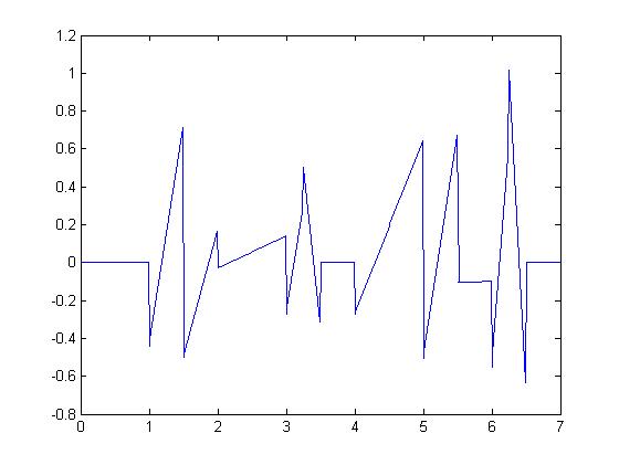
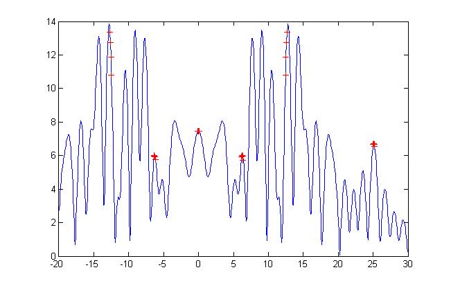
Figure 1: Plotted on the left is the sparse wavelet signal $f$ in (IV.1), while on the right is the magnitude of its Fourier transform and the measurements on $\Omega$.

The proposed algorithm is tested when the Fourier measurements of the signal $f$ are corrupted by random noises $\epsilon$,

$$h(\xi)=\hat{f}(\xi)+\epsilon(\xi),\ \ \xi\in\Omega.$$

In this case, sparsity locations obtained by Prony’s method in the algorithm are not necessarily integers, but it is observed that they are not far away from the sparsity locations of the signal $f$, when the signal-to-noise-ratio (SNR),

$$SNR=-20\log_{10}{\frac{\max_{\xi\in\Omega}|\epsilon(\xi)|}{\max_{\xi\in\Omega}|\hat{f}(\xi)|}}$$

is above 50 dB. Taking nearest integers of those locations may perfectly recover the sparsity positions $\{2,4\}$ for the scaling component of level $0$, $\{1,5\}$ for the wavelet component of level $0$, and $\{6,12\}$ for the wavelet component of level $1$. Then the signal $f$ can be reconstructed by the proposed algorithm approximately, see Figure 2.

Figure 2: The difference between the original signal and the reconstructed signal. In this figure, the reconstruction is generated by the proposed algorithm with modified Prony’s method, and the noise level on Fourier measurements is SNR=50 dB.

We also tested our proposed algorithm for two-dimensional wavelet signals with dilation ${\bf D}=\left(\hskip-3.61371pt\begin{array}[]{cc}0&-2\\ 1&0\\ \end{array}\hskip-3.61371pt\right)$. Presented on the left of Figure 3 is the amplitude of a sparse wavelet signal

$$\hskip-21.68121ptf(t_{1},t_{2}) \hskip-7.22743pt= \hskip-7.22743pta_{0}\phi(t_{1}-1,t_{2})+a_{1}\phi(t_{1}-2,t_{2}-3)$$ (IV.2)

$$\hskip-7.22743pt+ \hskip-7.22743ptb_{0}\psi(t_{1}-2,t_{2}-1)+b_{1}\psi(t_{1}-3,t_{2}-5),$$

where $a_{0},a_{1},b_{0},b_{1}\in[-1,1]\setminus(-0.1,0.1)$ are selected randomly, the scaling function is $\phi(t_{1},t_{2})=\chi_{[0,1)}(t_{1})\chi_{[0,1)}(t_{2})$, and the wavelet function is $\psi(t_{1},t_{2})=\chi_{[0,1)}(t_{1})(\chi_{[0,1/2)}(t_{1})-\chi_{[1/2,1)}(t_{2}))$. Our simulations show that the signal $f$ in (IV.2) can be reconstructed from its Fourier measurements on

$$\Omega=\Big{\{}\Big{(}\frac{\sqrt{2}}{64}n+2k,\frac{\sqrt{3}}{64}n+2l\Big{)}\pi,\ n=\pm 1,\pm 3\ {\rm and}\ k,l=0,1\Big{\}},$$ (IV.3)

which is plotted on the right of Figure 3.

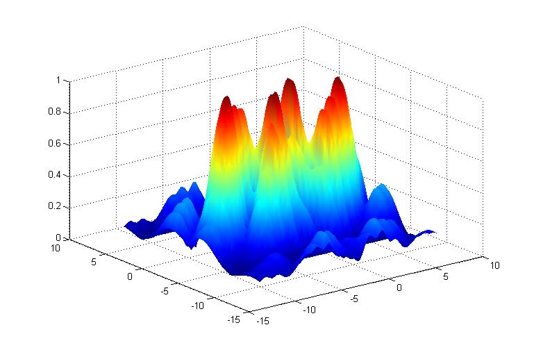
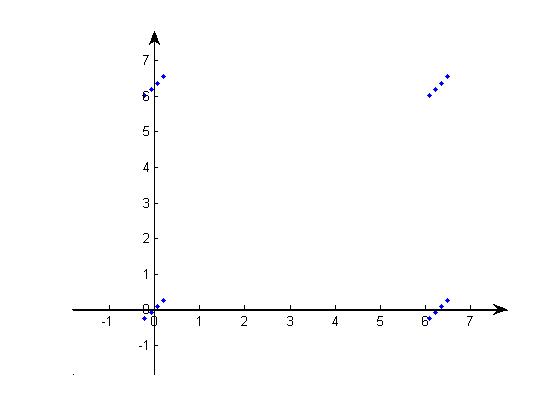
Figure 3: Fourier amplitudes of the signal $f$ in (IV.2) and the sampling set $\Omega$ in (IV.3) for sparse recovery.

V Conclusion

In this paper, we show that sparse wavelet signals of finite level can be reconstructed from their Fourier measurements on a deterministic sampling set, whose cardinality is independent on signal dimension and almost proportional to signal sparsity. A difficult problem on this aspect is exact reconstruction of signals having sparse wavelet-like (e.g. wavelet packet, framelet, curvelet, and shearlet) representations from their partial Fourier information ([27, 28, 29, 30, 31]).

References

• [1] I. Daubechies, Ten Lectures on Wavelets, SIAM, 1992.
• [2] S. Mallat, A Wavelet Tour of Signal Processing, Academic Press, 1999.
• [3] K. Gröchenig and W. R. Madych, Multiresolution analysis, Haar bases, and self-similar tilings of ${\mathbb{R}}^{n}$, IEEE Trans. Inform. Theory, 38(1992), 556–568.
• [4] A. Cohen and I. Daubechies, Non-separable bidimensional wavelet bases, Rev. Mat. Iberoamericana, 9(1993), 51–137.
• [5] J. S. Geronimo, D. P. Hardin and P. R. Massopust, Fractal functions and wavelet expansions based on several scaling functions, J. Approx. Theory, 78(1994), 373–401.
• [6] T. N. T. Goodman and S. L. Lee, Wavelets of multiplicity $r$, Trans. Amer. Math. Soc., 342(1994), 307–342.
• [7] P. N. Heller, Rank $M$ wavelets with $N$ vanishing moments, SIAM J. Matrix Anal. & Appl., 16(1995), 502–519.
• [8] B. Han and R. Q. Jia, Multivariate refinement equations and convergence of subdivision schemes, SIAM J. Math. Anal., 29(1998), 1177–1199.
• [9] N. Bi, X. Dai and Q. Sun, Construction of compactly supported $M$-band wavelets, Appl. Comp. Harmonic Anal., 6(1999), 113–131.
• [10] Q. Sun, N. Bi and D. Huang, An Introduction to Multiband Wavelets, Zhejiang University Press, 2001.
• [11] D. L. Donoho and M. Elad, Optimally sparse representation in general (nonorthogonal) dictionaries via $\ell^{1}$ minimization, Proc. Natl. Acad. Sci. U.S.A, 100(2003), 2197–2202.
• [12] E. J. Candes, J. Romberg and T. Tao, Robust uncertainty principles: exact signal reconstruction from highly incomplete frequency information, IEEE Trans. Inform. Theory, 52(2006), 489–509.
• [13] D. L. Donoho, Compressed sensing, IEEE Trans. Inform. Theory, 52(2006), 1289–1306.
• [14] R. Baraniuk, Compressive sensing, IEEE Signal Process. Mag., 24(2007), 118–124.
• [15] E. J. Candes and M. Wakin, An introduction to compressive sampling, IEEE Signal Process. Mag., 25(2008), 21–30.
• [16] Q. Sun, Recovery of sparsest signals via $\ell^{q}$-minimization, Appl. Comput. Harmonic Anal., 32(2012), 329–341.
• [17] J. Yang, Y. Zhang and W. Yin, A fast alternating direction method for TVL1-L2 signal reconstruction from partial Fourier data, IEEE J. Sel. Topics Signal Process., 4(2010), 288–297.
• [18] S. Foucart and H. Rauhut, A Mathematical Introduction to Compressive Sensing, Springer, 2013.
• [19] Y. Zhang and P. L. Dragotti, On the reconstruction of wavelet-sparse signals from partial Fourier information, IEEE Signal Proc. Letter, 22(2015), 1234–1238.
• [20] Y. Chen, C. Cheng and Q. Sun, Reconstruction of sparse multiband wavelet signals from Fourier measurements, Proceeding of the 11th International Conference on Sampling Theory and Applications (SAMPTA 2015), accepted.
• [21] R. Kumaresan, D. W. Tufts and L. L. Scharf, A Prony method for noisy data: choosing the signal components and selecting the order in exponential signal models, Proc. IEEE, 72(1984), 230–233.
• [22] L. L. Scharf, Statistical Signal Processing: Detection, Estimation, and Time Series, Prentice Hall, 1991.
• [23] M. M. Barbieri and P. Barone, A two-dimensional Prony’s method for spectral estimation, IEEE Trans. Signal Process., 40(1992), 2747–2756.
• [24] M. Vetterli, P. Marziliano, and T. Blu, Sampling signals with finite rate of innovation, IEEE Trans. Signal Process., 50(2002), 1417–1428.
• [25] M. R. Osborne and G. K. Smyth, A modified Prony algorithm for exponential function fitting, SIAM J. Sci. Comput. 16(2006), 119–138.
• [26] T. Peter and G. Plonka, A generalized Prony method for reconstruction of sparse sums of eigenfunctions of linear operators, Inverse Problems 29(2013), 025001
• [27] R. Coifman and M. V. Wickerhauser, Entropy-based algorithms for best basis selection, IEEE Trans. Inform. Theory, 38(1992), 713–718.
• [28] A. Ron and Z. Shen, Affine systems in $L^{2}({\mathbb{R}}^{d})$: the analysis of the analysis operator, J. Funct. Anal., 148(1997), 408–447.
• [29] E. J. Candes, L. Demanet, D. L. Donoho and L. Ying, Fast discrete curvelet transforms, SIAM J. Multiscale Model. Simul., 5(2006), 861–899.
• [30] C. K. Chui and Q. Sun, Affine frame decompositions and shift-invariant spaces, Appl. Comput. Harmonic Anal., 20(2006), 74–107.
• [31] G. Kutyniok and D. Labate, Shearlets: Multiscale Analysis for Multivariate Data, Springer, 2012.