Dynamical coupled-channels model of $K^{-}p$ reactions (II): Extraction of $\Lambda^{*}$ and $\Sigma^{*}$ hyperon resonances

Abstract

Resonance parameters (pole masses and residues) associated with the excited states of hyperons, $\Lambda^{*}$ and $\Sigma^{*}$, are extracted within a dynamical coupled-channels model developed recently by us [Phys. Rev. C 90, 065204 (2014)] through a comprehensive partial-wave analysis of the $K^{-}p\to\bar{K}N,\pi\Sigma,\pi\Lambda,\eta\Lambda,K\Xi$ data up to invariant mass $W=2.1$ GeV. We confirm the existence of resonances corresponding to most, if not all, of the four-star resonances rated by the Particle Data Group. We also find several new resonances, and in particular propose a possible existence of a new narrow $J^{P}=3/2^{+}$ $\Lambda$ resonance that couples strongly to the $\eta\Lambda$ channel. The $J^{P}=1/2^{-}$ $\Lambda$ resonances located below the $\bar{K}N$ threshold are also discussed. Comparing our extracted pole masses with the ones from a recent analysis by the Kent State University group, some significant differences in the extracted resonance parameters are found, suggesting the need of more extensive and accurate data of $K^{-}p$ reactions including polarization observables to eliminate such an analysis dependence of the resonance parameters. In addition, the determined large branching ratios of the decays of high-mass resonances to the $\pi\Sigma^{*}$ and $\bar{K}^{*}N$ channels also suggest the importance of the data of $2\to 3$ reactions such as $K^{-}p\to\pi\pi\Lambda$ and $K^{-}p\to\pi\bar{K}N$. Experiments on measuring cross sections and polarization observables of these fundamental reactions are highly desirable at hadron beam facilities such as J-PARC for establishing the $\Lambda^{*}$ and $\Sigma^{*}$ spectrum.

I Introduction

The spectra and structure of the excited baryons with light valence quarks ($u,d,s$) contain the information for understanding the non-perturbative aspects, confinements and chiral symmetry breaking, of Quantum Chromodynamics. The excited baryons are unstable and couple with meson-baryon continuum states to form nucleon resonances ($N^{*},\Delta^{*}$) with strangeness $S=0$ and hyperon resonances ($Y^{*}=\Lambda^{*},\Sigma^{*}$) with $S=-1$. Thus the extraction of these baryon resonances from the data of hadron-, photon-, and electron-induced meson-production reactions has long been an important task in the hadron physics. However, the hyperon resonances are much less understood than the nucleon resonances. This can be seen, for example, from the fact that only the Breit-Wigner masses and widths of the $\Lambda^{*}$ and $\Sigma^{*}$ resonances were listed by the Particle Data Group (PDG) before 2012 [exceptions are $\Sigma(1385)3/2^{+}$ and $\Lambda(1520)3/2^{-}$] pdg2012 . In contrast, the pole positions and residues of the $N^{*}$ and $\Delta^{*}$ resonances have been well determined by many analysis groups through detailed partial-wave analyses of $\pi N$ and $\gamma N$ reaction data. To improve the situation, a first comprehensive and systematic partial-wave analysis of $K^{-}p$ reaction data to extract $Y^{*}$ resonance parameters defined by poles of scattering amplitudes was made in 2013 by the Kent State University (KSU) group using an energy-independent approach zhang2013a , and subsequently they extracted the pole masses of $Y^{*}$ resonances by making an energy-dependent fit to their determined single-energy amplitudes zhang2013b . Recently, we have also made an extensive partial-wave analysis of $K^{-}p$ reactions within a dynamical-model approach knlskp1 . In this work, we present pole masses as well as residues of the $Y^{*}$ resonances extracted from our amplitudes determined in Ref. knlskp1 .

Our approach in Ref. knlskp1 is based on a dynamical coupled-channels (DCC) formulation that was developed in Ref. msl07 and applied extensively to the study of $N^{*}$ and $\Delta^{*}$ resonances jlms07 ; jlmss08 ; jklmss09 ; kjlms09-1 ; sjklms10 ; kjlms09-2 ; ssl2 ; knls10 ; knls13 ; kpi2pi13 . Schematically, we solve the following coupled integral equations for the $T$-matrix elements in each partial wave with strangeness $S=-1$,

$$T_{\beta,\alpha}(p_{\beta},p_{\alpha};W)=V_{\beta,\alpha}(p_{\beta},p_{\alpha};W)+\sum_{\delta}\int p^{2}dpV_{\beta,\delta}(p_{\beta},p;W)G_{\delta}(p;W)T_{\delta,\alpha}(p,p_{\alpha};W),$$ (1)

with

$$V_{\beta,\alpha}(p_{\beta},p_{\alpha};W)=v_{\beta,\alpha}(p_{\beta},p_{\alpha})+\sum_{Y^{*}}\frac{\Gamma^{\dagger}_{Y^{*},\beta}(p_{\beta})\Gamma_{Y^{*},\alpha}(p_{\alpha})}{W-M^{0}_{Y^{*}}},$$ (2)

where $W$ is the invariant mass of the reaction; the subscripts $\alpha,\beta,\delta$ denote the $\bar{K}N$, $\pi\Sigma$, $\pi\Lambda$, $\eta\Lambda$, and $K\Xi$ channels as well as the quasi-two-body $\pi\Sigma^{*}$ and $\bar{K}^{*}N$ channels that subsequently decay to the three-body $\pi\pi\Lambda$ and $\pi\bar{K}N$ channels; $G_{\delta}$ is the Green’s function of channel $\delta$; $M^{0}_{Y^{*}}$ is the mass of a bare excited hyperon state; $v_{\alpha,\beta}$ is defined by hadron-exchange mechanisms; and the bare vertex interaction $\Gamma_{Y^{*},\alpha}$ defines the $\alpha\to Y^{*}$ transition. By fitting the data of both unpolarized and polarized observables of the $K^{-}p\to\bar{K}N,\pi\Sigma,\pi\Lambda,\eta\Lambda,K\Xi$ reactions over the wide energy range from the threshold to invariant mass $W=2.1$ GeV, we have constructed two models, called Model A and Model B knlskp1 . The partial-wave amplitudes and the $S$-wave threshold parameters such as scattering lengths and effective ranges were then extracted from the constructed two models. The main objective of this paper is to present the $\Lambda^{*}$ and $\Sigma^{*}$ resonance parameters extracted from these two models and compare them with the results of the KSU analysis zhang2013b .

It is useful to mention here that the extracted resonance parameters are related to the data through the mechanisms defined in the Hamiltonian of our model. Thus it is possible to develop a theoretical understanding of the properties and structure of the extracted resonances in our approach. Such a feature is not available in the KSU approach and other similar approaches, in which the $K$ matrix or potential are parametrized purely phenomenologically by using some polynomials, and so on.

In Sec. II, we summarize notations, definitions, and formulas of the resonance parameters. In Sec. III, the resonance parameters (mass spectrum, residues, and branching ratios, etc.) extracted from our DCC models are presented for the $Y^{*}$ resonances located above the $\bar{K}N$ threshold, and the extracted mass spectra are compared with the one extracted from the KSU analysis. We then give a prediction for the $S$-wave $\Lambda$ resonances located below the $\bar{K}N$ threshold in Sec. IV, which would be interesting in relation to $\Lambda(1405)$, though it is a bit off the region of our current analysis. Summary and discussions on future developments are given in Sec. V.

II Resonance parameters

Table 1: The orbital angular momentum $(L)$ and total spin ($S$) of each $MB$ channel allowed in a given partial wave. In the first column, partial waves are denoted with the conventional notation $l_{I2J}$ as well as ($I$,$J^{P}$).

$l_{I2J}$ $(I,J^{P})$	$(L,S)$ of the considered partial waves
	$\bar{K}N$	$\pi\Sigma$	$\pi\Lambda$	$\eta\Lambda$	$K\Xi$	$\pi\Sigma^{*}$		$\bar{K}^{*}N$
						$(\pi\Sigma^{*})_{1}$	$(\pi\Sigma^{*})_{2}$	$(\bar{K}^{*}N)_{1}$	$(\bar{K}^{*}N)_{2}$	$(\bar{K}^{*}N)_{3}$
$S_{01}$ $(0,\textstyle{\frac{1}{2}}^{-})$	($0,\textstyle{\frac{1}{2}}$)	($0,\textstyle{\frac{1}{2}}$)	–	($0,\textstyle{\frac{1}{2}}$)	($0,\textstyle{\frac{1}{2}}$)	($2,\textstyle{\frac{3}{2}}$)	–	($0,\textstyle{\frac{1}{2}}$)	($2,\textstyle{\frac{3}{2}}$)	–
$S_{11}$ $(1,\textstyle{\frac{1}{2}}^{-})$	($0,\textstyle{\frac{1}{2}}$)	($0,\textstyle{\frac{1}{2}}$)	($0,\textstyle{\frac{1}{2}}$)	–	($0,\textstyle{\frac{1}{2}}$)	($2,\textstyle{\frac{3}{2}}$)	–	($0,\textstyle{\frac{1}{2}}$)	($2,\textstyle{\frac{3}{2}}$)	–
$P_{01}$ $(0,\textstyle{\frac{1}{2}}^{+})$	($1,\textstyle{\frac{1}{2}}$)	($1,\textstyle{\frac{1}{2}}$)	–	($1,\textstyle{\frac{1}{2}}$)	($1,\textstyle{\frac{1}{2}}$)	($1,\textstyle{\frac{3}{2}}$)	–	($1,\textstyle{\frac{1}{2}}$)	($1,\textstyle{\frac{3}{2}}$)	–
$P_{03}$ $(0,\textstyle{\frac{3}{2}}^{+})$	($1,\textstyle{\frac{1}{2}}$)	($1,\textstyle{\frac{1}{2}}$)	–	($1,\textstyle{\frac{1}{2}}$)	($1,\textstyle{\frac{1}{2}}$)	($1,\textstyle{\frac{3}{2}}$)	($3,\textstyle{\frac{3}{2}}$)	($1,\textstyle{\frac{1}{2}}$)	($1,\textstyle{\frac{3}{2}}$)	($3,\textstyle{\frac{3}{2}}$)
$P_{11}$ $(1,\textstyle{\frac{1}{2}}^{+})$	($1,\textstyle{\frac{1}{2}}$)	($1,\textstyle{\frac{1}{2}}$)	($1,\textstyle{\frac{1}{2}}$)	–	($1,\textstyle{\frac{1}{2}}$)	($1,\textstyle{\frac{3}{2}}$)	–	($1,\textstyle{\frac{1}{2}}$)	($1,\textstyle{\frac{3}{2}}$)	–
$P_{13}$ $(1,\textstyle{\frac{3}{2}}^{+})$	($1,\textstyle{\frac{1}{2}}$)	($1,\textstyle{\frac{1}{2}}$)	($1,\textstyle{\frac{1}{2}}$)	–	($1,\textstyle{\frac{1}{2}}$)	($1,\textstyle{\frac{3}{2}}$)	($3,\textstyle{\frac{3}{2}}$)	($1,\textstyle{\frac{1}{2}}$)	($1,\textstyle{\frac{3}{2}}$)	($3,\textstyle{\frac{3}{2}}$)
$D_{03}$ $(0,\textstyle{\frac{3}{2}}^{-})$	($2,\textstyle{\frac{1}{2}}$)	($2,\textstyle{\frac{1}{2}}$)	–	($2,\textstyle{\frac{1}{2}}$)	($2,\textstyle{\frac{1}{2}}$)	($0,\textstyle{\frac{3}{2}}$)	($2,\textstyle{\frac{3}{2}}$)	($2,\textstyle{\frac{1}{2}}$)	($0,\textstyle{\frac{3}{2}}$)	($2,\textstyle{\frac{3}{2}}$)
$D_{05}$ $(0,\textstyle{\frac{5}{2}}^{-})$	($2,\textstyle{\frac{1}{2}}$)	($2,\textstyle{\frac{1}{2}}$)	–	($2,\textstyle{\frac{1}{2}}$)	($2,\textstyle{\frac{1}{2}}$)	($2,\textstyle{\frac{3}{2}}$)	($4,\textstyle{\frac{3}{2}}$)	($2,\textstyle{\frac{1}{2}}$)	($2,\textstyle{\frac{3}{2}}$)	($4,\textstyle{\frac{3}{2}}$)
$D_{13}$ $(1,\textstyle{\frac{3}{2}}^{-})$	($2,\textstyle{\frac{1}{2}}$)	($2,\textstyle{\frac{1}{2}}$)	($2,\textstyle{\frac{1}{2}}$)	–	($2,\textstyle{\frac{1}{2}}$)	($0,\textstyle{\frac{3}{2}}$)	($2,\textstyle{\frac{3}{2}}$)	($2,\textstyle{\frac{1}{2}}$)	($0,\textstyle{\frac{3}{2}}$)	($2,\textstyle{\frac{3}{2}}$)
$D_{15}$ $(1,\textstyle{\frac{5}{2}}^{-})$	($2,\textstyle{\frac{1}{2}}$)	($2,\textstyle{\frac{1}{2}}$)	($2,\textstyle{\frac{1}{2}}$)	–	($2,\textstyle{\frac{1}{2}}$)	($2,\textstyle{\frac{3}{2}}$)	($4,\textstyle{\frac{3}{2}}$)	($2,\textstyle{\frac{1}{2}}$)	($2,\textstyle{\frac{3}{2}}$)	($4,\textstyle{\frac{3}{2}}$)
$F_{05}$ $(0,\textstyle{\frac{5}{2}}^{+})$	($3,\textstyle{\frac{1}{2}}$)	($3,\textstyle{\frac{1}{2}}$)	–	($3,\textstyle{\frac{1}{2}}$)	($3,\textstyle{\frac{1}{2}}$)	($1,\textstyle{\frac{3}{2}}$)	($3,\textstyle{\frac{3}{2}}$)	($3,\textstyle{\frac{1}{2}}$)	($1,\textstyle{\frac{3}{2}}$)	($3,\textstyle{\frac{3}{2}}$)
$F_{07}$ $(0,\textstyle{\frac{7}{2}}^{+})$	($3,\textstyle{\frac{1}{2}}$)	($3,\textstyle{\frac{1}{2}}$)	–	($3,\textstyle{\frac{1}{2}}$)	($3,\textstyle{\frac{1}{2}}$)	($3,\textstyle{\frac{3}{2}}$)	($5,\textstyle{\frac{3}{2}}$)	($3,\textstyle{\frac{1}{2}}$)	($3,\textstyle{\frac{3}{2}}$)	($5,\textstyle{\frac{3}{2}}$)
$F_{15}$ $(1,\textstyle{\frac{5}{2}}^{+})$	($3,\textstyle{\frac{1}{2}}$)	($3,\textstyle{\frac{1}{2}}$)	($3,\textstyle{\frac{1}{2}}$)	–	($3,\textstyle{\frac{1}{2}}$)	($1,\textstyle{\frac{3}{2}}$)	($3,\textstyle{\frac{3}{2}}$)	($3,\textstyle{\frac{1}{2}}$)	($1,\textstyle{\frac{3}{2}}$)	($3,\textstyle{\frac{3}{2}}$)
$F_{17}$ $(1,\textstyle{\frac{7}{2}}^{+})$	($3,\textstyle{\frac{1}{2}}$)	($3,\textstyle{\frac{1}{2}}$)	($3,\textstyle{\frac{1}{2}}$)	–	($3,\textstyle{\frac{1}{2}}$)	($3,\textstyle{\frac{3}{2}}$)	($5,\textstyle{\frac{3}{2}}$)	($3,\textstyle{\frac{1}{2}}$)	($3,\textstyle{\frac{3}{2}}$)	($5,\textstyle{\frac{3}{2}}$)

Since the method for extracting the resonance parameters within the considered dynamical model has been explained in detail in Refs. ssl ; ssl2 ; knls13 , here we just summarize formulas that are needed for the presentations in this paper.

Consider the $MB\to M^{\prime}B^{\prime}$ reactions in the center-of-mass system, where $MB$ and $M^{\prime}B^{\prime}$ are the initial and final meson-baryon states. With the normalization $\langle{\vec{k}}|{\vec{k}^{{}^{\prime}}}\rangle=\delta(\vec{k}-\vec{k}^{{}^{\prime}})$ for plane waves, the on-shell $S$ matrix elements at the total scattering energy $W$ are given for each partial wave by

$$S_{M^{\prime}B^{\prime},MB}(W)=\delta_{M^{\prime}B^{\prime},MB}+2iF_{M^{\prime}B^{\prime},MB}(W).$$ (3)

Here the index $MB$ ($M^{\prime}B^{\prime}$) also specifies quantum numbers associated with the channel $MB$ ($M^{\prime}B^{\prime}$), namely, the orbital angular momentum ($L$), total spin ($S$), total angular momentum ($J$), parity ($P$), and isospin ($I$). The values of these quantum numbers for the considered meson-baryon channels are summarized in Table 1. The on-shell scattering amplitudes $F_{M^{\prime}B^{\prime},MB}(W)$ are related to the $T$-matrix elements [Eq. (1)] as

$$F_{M^{\prime}B^{\prime},MB}(W)=-[\rho_{M^{\prime}B^{\prime}}(k_{M^{\prime}B^{\prime}}^{\text{on}};W)]^{1/2}T_{M^{\prime}B^{\prime},MB}(k_{M^{\prime}B^{\prime}}^{\text{on}},k_{MB}^{\text{on}};W)[\rho_{MB}(k_{MB}^{\text{on}};W)]^{1/2},$$ (4)

with

$$\rho_{MB}(k;W)=\pi\frac{kE_{M}(k)E_{B}(k)}{W},$$ (5)

where $E_{a}(k)=\sqrt{m_{a}^{2}+k^{2}}$ is the energy of a particle $a$ with the mass $m_{a}$ and the three-momentum $\vec{k}$ ($k\equiv|\vec{k}|$). For a given $W$, which can be complex, the on-shell momentum for the channel $MB$, $k_{MB}^{\mathrm{on}}$, is defined by

$$W=E_{M}(k_{MB}^{\mathrm{on}})+E_{B}(k_{MB}^{\mathrm{on}}).$$ (6)

The formulas and procedures to calculate the $T$-matrix elements within our DCC model are fully explained in Ref. knlskp1 , and thus we will not repeat them here.

As the energy $W$ approaches a pole position $M_{R}$ in the complex $W$ plane, the scattering amplitudes take the following form,

$$F_{M^{\prime}B^{\prime},MB}(W\to M_{R})=-\frac{R_{M^{\prime}B^{\prime},MB}}{W-M_{R}}+B_{M^{\prime}B^{\prime},MB},$$ (7)

where $R_{M^{\prime}B^{\prime},MB}$ is the residue of $F_{M^{\prime}B^{\prime},MB}(W)$ at the resonance pole $M_{R}$, and $B_{M^{\prime}B^{\prime},MB}$ is the “background” contribution. Both $R_{M^{\prime}B^{\prime},MB}$ and $B_{M^{\prime}B^{\prime},MB}$ are constant and in general complex. The pole position ($M_{R}$) and the residue ($R_{M^{\prime}B^{\prime},MB}$) are fundamental quantities that characterize the resonance. In fact, within the resonance theory based on the Gamow vectors (see, e.g., Ref. madrid ), $M_{R}$ is equivalent to a complex energy eigenvalue of the total Hamiltonian of the considered system under the outgoing wave boundary conditions, and the (square-root of) residues can be associated with the strength of the transition from the resonance to a scattering state of $MB$ and/or $M^{\prime}B^{\prime}$ channel.

Practically, within our approach the value of $M_{R}$ for a resonance can be obtained as a solution of the following equation with respect to $W$ ssl ; ssl2 ; knls13 :

$$\mathrm{det}[D^{-1}(W)]=0,$$ (8)

with $D^{-1}(W)$ being the inverse of the dressed $Y^{*}$ resonance propagators. It is defined by knlskp1

$$[D^{-1}(W)]_{n,m}=W\delta_{n,m}-[M_{Y^{*}}(W)]_{n,m}.$$ (9)

The resonance mass matrix $M_{Y^{*}}(W)$ is given by

$$[M_{Y^{*}}(W)]_{n,m}=M_{Y_{n}^{*}}^{0}\delta_{n,m}+[\Sigma_{Y^{*}}(W)]_{n,m},$$ (10)

where $M_{Y_{n}^{*}}^{0}$ is the mass of the $n$th bare $Y^{*}$ state in a given partial wave, and $\Sigma_{Y^{*}}(W)$ is the matrix for the $Y^{*}$ self energy knlskp1 . Solving Eq. (8) is nothing but searching for poles of the resonance propagator in the complex $W$ plane. The nonlinearity and multivaluedness of $\Sigma_{Y^{*}}(W)$ originating from the multichannel reaction dynamics make the relation between bare states and physical resonances highly nontrivial. In fact, as has been demonstrated in Ref. sjklms10 , a naive one-to-one correspondence between bare states and physical resonances does not hold in general within a multichannel reaction system.

It is noted sjklms10 that Eqs. (8)-(10) give the exact resonance pole masses of the full scattering amplitudes (4) as far as the bare $Y^{*}$ state(s) is introduced for the considered partial wave. Otherwise, one must search for resonance poles in the complex $W$ plane directly from the original full scattering amplitudes (4). Since at least one bare $Y^{*}$ state has been introduced for each partial wave in our two models, Model A and Model B constructed in Ref. knlskp1 , we just use Eq. (8) to search for resonance poles.

The residues $R_{M^{\prime}B^{\prime},MB}$ defined in Eq. (7) can be calculated by using the definition:

$$R_{M^{\prime}B^{\prime},MB}=\frac{1}{2\pi i}\oint_{C_{M_{R}}}dW[-F_{M^{\prime}B^{\prime},MB}(W)],$$ (11)

where $C_{M_{R}}$ is an appropriate closed-path in the neighborhood of the point $W=M_{R}$, circling $W=M_{R}$ in a counterclockwise manner.

As for the partial waves for which bare $Y^{*}$ state(s) is introduced, however, $R_{M^{\prime}B^{\prime},MB}$ can also be calculated with ssl ; ssl2 ; knls13

$$R_{M^{\prime}B^{\prime},MB}=[\rho_{M^{\prime}B^{\prime}}(k_{M^{\prime}B^{\prime}}^{\text{on}};M_{R})]^{1/2}\bar{\Gamma}^{R}_{M^{\prime}B^{\prime},Y^{*}}(k_{M^{\prime}B^{\prime}}^{\text{on}};M_{R})\bar{\Gamma}^{R}_{Y^{*},MB}(k_{MB}^{\text{on}};M_{R})[\rho_{MB}(k_{MB}^{\text{on}};M_{R})]^{1/2}.$$ (12)

Here $\bar{\Gamma}^{R}_{MB,Y^{*}}(k;W)$ and $\bar{\Gamma}^{R}_{Y^{*},MB}(k;W)$ are the dressed $Y^{*}\to MB$ and $MB\to Y^{*}$ vertices, respectively, given by

$$\bar{\Gamma}^{R}_{MB,Y^{*}}(k;W) = \sum_{n}\chi_{n}\bar{\Gamma}_{MB,Y_{n}^{*}}(k;W),$$ (13)

$$\bar{\Gamma}^{R}_{Y^{*},MB}(k;W) = \sum_{n}\chi_{n}\bar{\Gamma}_{Y_{n}^{*},MB}(k;W),$$ (14)

where $\bar{\Gamma}_{MB,Y_{n}^{*}}(k;W)$ and $\bar{\Gamma}_{Y_{n}^{*},MB}(k;W)$, of which expressions are explicitly given in Ref. knlskp1 , are the dressed vertices for the $n$th bare $Y^{*}$ state; and the coefficient $\chi_{n}$ satisfies

$$[D(W)]_{n,m}=\frac{\chi_{n}\chi_{m}}{W-M_{R}}+(\textrm{regular~{}terms~{}at~{}}W=M_{R}),$$ (15)

in the neighborhood of the point $W=M_{R}$, and

$$\sum_{m}[D^{-1}(M_{R})]_{n,m}\chi_{m}=0.$$ (16)

We have confirmed that Eq. (12) indeed gives exactly the same value as calculated from using Eq. (11).

It should be emphasized here that the coefficient $\chi_{n}$ represents the $n$th bare-state component of the fully dressed $Y^{*}$ resonance. In other words, it indicates the meson-baryon contents of a resonance within the dynamical reaction models ttm . For example, for the case that one bare state is contained, the coefficient $\chi\equiv\chi_{1}$ is given explicitly as

$$\chi=\left(1-\left.\frac{d\Sigma_{Y^{*}}(W)}{dW}\right|_{W=M_{R}}\right)^{-1/2}.$$ (17)

This is nothing but the square root of the (complex) wave function renormalization constant $Z$ for the bare state ttm .

III $\Lambda^{*}$ and $\Sigma^{*}$ resonances above the $\bar{K}N$ threshold

With the formulas described in Sec. II and the analytic continuation method developed in Refs. ssl ; ssl2 , we have extracted the parameters of the $\Lambda^{*}$ and $\Sigma^{*}$ resonances from Model A and Model B constructed in Ref. knlskp1 . In this section, we present the results for the resonances found in the energy region above the $\bar{K}N$ threshold.

III.1 Resonance masses

Table 2: Extracted complex pole masses ($M_{R}$) for the $\Lambda^{*}$ and $\Sigma^{*}$ resonances found in the energy region above the $\bar{K}N$ threshold. The masses are listed as $\bm{(}{\rm Re}(M_{R}),-{\rm Im}(M_{R})\bm{)}$ together with their deduced uncertainties. The resonance poles are searched in the complex $W$ region with $m_{\bar{K}}+m_{N}\leq{\rm Re}(W)\leq 2.1$ GeV and $0\leq-{\rm Im}(W)\leq 0.2$ GeV, and all of the resonances listed are located in the complex $W$ Riemann surface nearest to the physical real $W$ axis.

		$M_{R}$ (MeV)
	$J^{P}(l_{I2J})$	Model A	Model B
$\Lambda$-baryons	$1/2^{-}(S_{01})$	(1669${}^{+3}_{-8}$, 9${}^{+9}_{-1}$)	(1512${}^{+1}_{-1}$,185${}^{+1}_{-2}$)
			(1667${}^{+1}_{-2}$,12${}^{+3}_{-1}$)
	$1/2^{+}(P_{01})$	(1544${}^{+3}_{-3}$, 56${}^{+6}_{-1}$)	(1548${}^{+5}_{-6}$, 82${}^{+7}_{-7}$)
		(2097${}^{+40}_{-1}$, 83${}^{+32}_{-6}$)	(1841${}^{+3}_{-4}$, 31${}^{+3}_{-2}$)
	$3/2^{+}(P_{03})$	(1859${}^{+5}_{-7}$, 56${}^{+10}_{-2}$)	(1671${}^{+2}_{-8}$, 5${}^{+11}_{-2}$)
	$3/2^{-}(D_{03})$	(1517${}^{+4}_{-4}$, 8${}^{+5}_{-4}$)	(1517${}^{+4}_{-3}$, 8${}^{+6}_{-6}$)
		(1697${}^{+6}_{-6}$, 33${}^{+7}_{-7}$)	(1697${}^{+6}_{-5}$, 37${}^{+7}_{-7}$)
	$5/2^{-}(D_{05})$	(1766${}^{+37}_{-34}$,106${}^{+47}_{-31}$)	(1924${}^{+52}_{-24}$, 45${}^{+57}_{-17}$)
		(1899${}^{+35}_{-37}$, 40${}^{+50}_{-17}$)
	$5/2^{+}(F_{05})$	(1824${}^{+2}_{-1}$, 39${}^{+1}_{-1}$)	(1821${}^{+1}_{-1}$, 32${}^{+1}_{-1}$)
	$7/2^{+}(F_{07})$	(1757, 73)	(2041${}^{+80}_{-82}$,119${}^{+57}_{-17}$)
$\Sigma$-baryons	$1/2^{-}(S_{11})$	(1704${}^{+3}_{-6}$, 43${}^{+7}_{-2}$)	(1551${}^{+2}_{-9}$,188${}^{+6}_{-1}$)
			(1940${}^{+2}_{-2}$, 86${}^{+2}_{-2}$)
	$1/2^{+}(P_{11})$	(1547${}^{+111}_{-59}$, 92${}^{+43}_{-39}$)	(1457${}^{+5}_{-1}$, 39${}^{+1}_{-4}$)
		(1706${}^{+67}_{-60}$, 51${}^{+79}_{-42}$)	(1605${}^{+2}_{-4}$, 96${}^{+1}_{-5}$)
			(2014${}^{+6}_{-13}$, 70${}^{+14}_{-1}$)
	$3/2^{-}(D_{13})$	(1607${}^{+13}_{-11}$,126${}^{+15}_{-9}$)	(1492${}^{+4}_{-7}$, 69${}^{+4}_{-7}$)
		(1669${}^{+7}_{-7}$, 32${}^{+5}_{-7}$)	(1672${}^{+5}_{-10}$, 33${}^{+3}_{-3}$)
	$5/2^{-}(D_{15})$	(1767${}^{+2}_{-2}$, 64${}^{+2}_{-1}$)	(1765${}^{+2}_{-1}$, 64${}^{+3}_{-1}$)
	$5/2^{+}(F_{15})$	(1890${}^{+3}_{-2}$, 49${}^{+2}_{-3}$)	(1695${}^{+20}_{-77}$, 97${}^{+50}_{-44}$)
	$7/2^{+}(F_{17})$	(2025${}^{+10}_{-5}$, 65${}^{+3}_{-12}$)	(2014${}^{+12}_{-1}$,103${}^{+3}_{-9}$)

The resonance masses (pole positions), $M_{R}$, are the solutions of Eq. (8) on the complex $W$ plane. In general, the physical observables are less influenced by the resonances with very large widths, and thus the information for such resonances extracted from fitting the data are less reliable. Therefore, following our previous study of $N^{*}$ and $\Delta^{*}$ resonances knls13 , we examine only the resonances with total width less than 400 MeV [the total width is defined as $\Gamma^{\rm tot}=-2{\rm Im}(M_{R})$]. We also do not search for resonances with ${\rm Re}(M_{R})>2.1$ GeV. With these criteria, 18 (20) resonances with the spin-parity $J^{P}=1/2^{\pm},3/2^{\pm},5/2^{\pm},7/2^{+}$ are extracted within the Model A (Model B) in the energy region above the $\bar{K}N$ threshold. All of these resonances are located in the Riemann surface which is nearest to the physical real $W$ axis. The extracted resonance masses $M_{R}$ are listed in Table 2.

Because of the “incompleteness” of the current database of the $K^{-}p$ reactions, as discussed in Ref. knlskp1 , there are expected to be different solutions of partial-wave analysis with similar $\chi^{2}$ minima. We indicate in Table 2 our estimates of the uncertainties of the extracted resonance masses originating from such “indistinguishable” solutions within the available $K^{-}p$ reaction data. Similar uncertainties also occur in the analyses of the $\pi N$ and $\gamma N$ reactions, as discussed, for example, in Ref. bg2012 . In principle, the uncertainties in a dynamical coupled-channels analysis, such as this work, should be evaluated by varying all parameters of the starting Hamiltonian simultaneously in wide ranges around the values determined in the $\chi^{2}$ fits. Such a procedure is however practically not feasible since solving the coupled-channels integral equations (1) and (2) is rather time consuming and the parameter space of the constructed models is rather large.

Instead, we take a more tractable procedure described as follows. For each partial wave listed in Table 1, additional parameters, $\delta M_{Y_{n}^{*}}$, are added to the diagonal elements of the mass matrix [Eq.(10)]:

$$[M_{Y^{*}}(W)]_{n,m}\to[M_{Y^{*}}(W)]_{n,m}+\delta M_{Y^{*}_{n}}\delta_{n,m},$$ (18)

where $\delta M_{Y_{n}^{*}}$ are taken to be complex. We then refit the $K^{-}p$ reaction data listed in Table II of Ref. knlskp1 by choosing randomly the initial values of $\delta M_{Y_{n}^{*}}$. By keeping the model parameters in the Hamiltonian fixed and varying only the additional $\delta M_{Y_{n}^{*}}$ parameters with a gradient minimization procedure, we obtain a set of $\delta M_{Y_{n}^{*}}$ values for the chosen initial values. This minimization procedure is repeated about $10^{5}$ times for a wide range of initial $\delta M_{Y_{n}^{*}}$ values. We then pick up the solutions that give almost the same $\chi^{2}$ values as the original one ($\chi^{2}_{\textrm{org}}$) from Model A or B by setting the condition $|(\chi^{2}-\chi^{2}_{\textrm{org}})/\chi^{2}_{\textrm{org}}|\leq 1\%$. About 20$\%$ of the solutions meet this condition. Note that this procedure of determining the range of allowed $\delta M_{Y_{n}^{*}}$ values, i.e., Monte Carlo sampling combined with gradient minimization, is motivated by the one taken in Ref. shkl11 in determining the multipole amplitudes of the $\gamma p\to K^{+}\Lambda$ reaction. The uncertainties of the resonance masses are then determined from the range of pole values found by solving Eq. (8) in which $\delta M_{Y_{n}^{*}}$ is varied over the allowed range. The resulting uncertainties are listed in Table 2. Overall, the magnitude of our estimated uncertainties are consistent with the one listed in PDG pdg2014 . One exception is the mass for the $J^{P}=7/2^{+}$ $\Lambda$ resonance in Model A, for which the uncertainty is not assigned because it is too large to be meaningful. Several resonances, e.g., $J^{P}=3/2^{-}$ $\Lambda$ resonances, appear in both Models A and B to have almost the same central value and uncertainty for $M_{R}$. Resonances that are found in only either of Model A or B basically have large uncertainty in their masses. However, some exceptions also exist, for example, the first $J^{P}=1/2^{-}$ $\Lambda$ resonance in Model B, for which the counterpart is not found in Model A but the uncertainty for its mass is rather small. The existence of such exceptions implies that the dynamical contents of our two models are rather different from each other, yet they are hard to be distinguished with the current $K^{-}p$ reaction data included in our fits due to its “incompleteness” mentioned above and explained in Ref. knlskp1 .

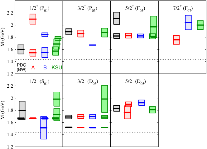
Figure 1: (Color online) Mass spectrum of $\Lambda^{*}$ resonances above the $\bar{K}N$ threshold. For each $\Lambda^{*}$, $\mathrm{Re}(M_{R})$ together with the $\mathrm{Re}(M_{R})\pm[-\mathrm{Im}(M_{R})]$ band is plotted, where the length of the band, $-2\mathrm{Im}(M_{R})$, corresponds to the total width of the resonance. The spin and parity of the resonances are denoted as $J^{P}$ with $P=\pm$, and also specified by the quantum number ($l_{I2J}$) of the associated $\bar{K}N$ partial-wave amplitudes. The horizontal dotted lines represent the $\bar{K}N$ threshold. The results from Model A and Model B constructed in Ref. knlskp1 are compared with the ones from the KSU analysis zhang2013b . The so-called Breit-Wigner masses and widths of the four- and three-star resonances rated by PDG pdg2014 are also presented.

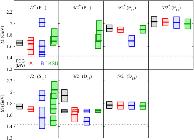
Figure 2: (Color online) Mass spectrum of $\Sigma^{*}$ resonances above the $\bar{K}N$ threshold. See the caption of Fig. 1 for the description of the figure.

The $\Lambda^{*}$ and $\Sigma^{*}$ mass spectra extracted from Models A and B are compared with the results from the KSU analysis zhang2013b in Figs. 1 and 2, respectively. In the same figures, we also indicate the mass spectra of the four- and three-star resonances assigned by PDG pdg2014 . It should be noted that the mass spectra listed by PDG pdg2014 are evaluated using the masses and widths from the the Breit-Wigner parametrization of the scattering amplitudes. It is now well recognized that the resonance parameters obtained with the Breit-Wigner parametrizations are not trivially related to the ones determined at the resonance pole positions. Thus the PDG values given in Figs. 1 and 2 are just for an additional reference in assessing the model dependence of the analyses.

We see in Figs. 1 and 2 that the results from our two models and the KSU analysis show an excellent agreement for several resonances. However, large discrepancies are also seen between the three results, and those need to be resolved. This of course reflects the fact that the existing $K^{-}p$ reaction data are not sufficient to constrain the mass spectrum of $Y^{*}$ resonances (see Ref. knlskp1 for the current situation of the world data for the $K^{-}p$ reactions). More extensive and accurate data including polarization observables are highly desirable to get convergent results.

It is interesting to see that our two models and the KSU analysis have low-lying $\Sigma^{*}$ resonances with $\mathrm{Re}(M_{R})<1.6$ GeV in $S_{11}$, $P_{11}$, and $D_{13}$. They may correspond to one- and two-star resonances assigned by PDG (but are not indicated in Fig. 2). To establish such low-lying resonances, more data near the $\bar{K}N$ threshold are definitely needed.

In the following, we further discuss each of resonances shown in Figs. 1 and 2:

$\bm{S_{01}[\Lambda(1/2^{-})]}$

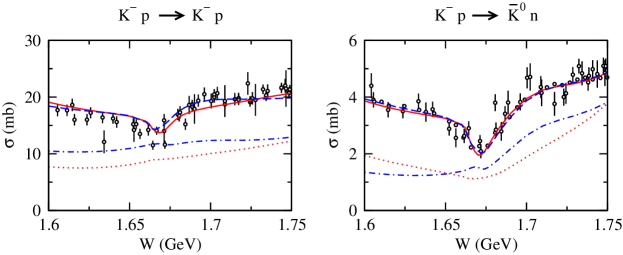
Figure 3: (Color online) The $K^{-}p\to K^{-}p$ and $K^{-}p\to\bar{K}^{0}n$ total cross sections at the energies near $W\sim 1.67$ GeV. Red solid (blue dashed) curves are the full results from Model A (Model B), while red dotted (blue dashed-dotted) curves are the results for which the $S_{01}$ resonance contributions are turned off.

Our two models, Model A and Model B, and the KSU analysis all give a narrow resonance with $\mathrm{Re}(M_{R})\sim 1.67$ GeV (Fig. 1). It can be identified with the four-star $\Lambda(1670)1/2^{-}$ of PDG (narrow black bar in the left-most column). As discussed in our previous paper knlskp1 , this resonance is responsible for the sharp peak in the $K^{-}p\to\eta\Lambda$ total cross section near the threshold. This strong near-threshold effect is similar to that of $N^{*}(1535)1/2^{-}$ resonance on the $\pi N\to\eta N$ reaction. The $\Lambda(1670)1/2^{-}$ is also found to be responsible for a dip in the $K^{-}p\to\bar{K}N$ total cross sections at $W\sim 1.67$ GeV. This is presented in Fig. 3. Other than the agreement in extracting the $\Lambda(1670)1/2^{-}$ resonance between the three analyses, a broad resonance at $\mathrm{Re}(M_{R})\sim 1.5$ GeV is found in Model B and two additional resonances are found at higher energies in the KSU analysis.

$\bm{P_{01}[\Lambda(1/2^{+})]}$

The lowest resonance at $\mathrm{Re}(M_{R})\sim 1.55$ GeV shows an agreement between the three analyses. This resonance would correspond to $\Lambda(1600)1/2^{+}$, a three-star resonance rated by PDG. Clearly, the higher resonances are not well determined.

$\bm{P_{03}[\Lambda(3/2^{+})]}$

A resonance at $\mathrm{Re}(M_{R})\sim 1.86$ GeV is found in Model A and the KSU analysis, but not in Model B. Thus the current data are not sufficient to establish this state model independently. If this resonance corresponds to the four-star $\Lambda(1890)3/2^{+}$ of PDG, then this is one example indicating that a four-star resonance rated by PDG using the Breit-Wigner parameters is not confirmed by the analyses in which the resonance parameters are extracted at pole positions.

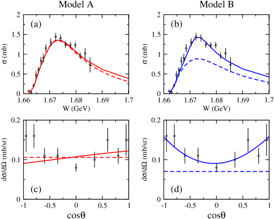
Figure 4: (Color online) Total cross section near the threshold (upper panels) and differential cross section at $W=1672$ MeV (lower panels) for the $K^{-}p\to\eta\Lambda$ reaction. Left panels (right panels) are the results from Model A (Model B). Solid curves are the full results, while the dashed curves are the contribution from the $S_{01}$ partial wave only. For Model B, the difference between the solid and dashed curves almost comes from the $P_{03}$ partial wave dominated by the new narrow $J^{P}=3/2^{+}$ $\Lambda$ resonance with $M_{R}=1671^{+2}_{-8}-i(5^{+11}_{-2})$ MeV.

The main feature of Model B is to have a new narrow $\Lambda$ resonance with $M_{R}=1671^{+2}_{-8}-i(5^{+11}_{-2})$ MeV. It locates in the energy region close to the $S_{01}$ resonance $\Lambda(1670)1/2^{-}$ discussed above. As already discussed in our previous paper knlskp1 , the evidence of this new narrow resonance could be seen from the $K^{-}p\to\eta\Lambda$ cross sections near the threshold. To see this, we compare the contributions from this resonance and the $S_{01}$ resonance $\Lambda(1670)1/2^{-}$ to the cross sections. As shown in Fig. 4(a), the peak of the $K^{-}p\to\eta\Lambda$ total cross section near the threshold calculated from Model A is completely dominated by the contribution from the $S_{01}$ partial wave that is almost entirely due to the $\Lambda(1670)1/2^{-}$ resonance. On the other hand, we see in Fig. 4(b) that the contribution of the $S_{01}$ partial wave in Model B is just about 60 %, and the remaining 40 % come almost entirely from the $P_{03}$ partial wave that contains this new narrow resonance. Since both models reproduce the total cross section very well, the existence of this new narrow $J^{P}=3/2^{+}$ $\Lambda$ resonance cannot be established only by considering the total cross sections. To get a deeper insight, it is necessary to at least examine its effects on the differential cross sections. The $K^{-}p\to\eta\Lambda$ differential cross section data near the threshold ($W\sim 1.67$ GeV) show a clear concave-up angular dependence that cannot be described by the $S$-wave amplitudes. We see in Fig. 4(c) that the results (solid curve) from Model A, which is mainly the $S_{01}$ wave (dashed curve), do not reproduce the angular dependence well. On the other hand, the new narrow $J^{P}=3/2^{+}$ $\Lambda$ resonance extracted within Model B is found to be responsible for the reproduction of the differential cross section data. This is shown in Fig. 4(d), suggesting that the angular dependence of the data seems to favor the existence of this new resonance.

$\bm{D_{03}[\Lambda(3/2^{-})]}$

The first and second resonances in the $D_{03}$ partial wave extracted from Models A and B and KSU analysis agree very well. Compared with the PDG values (the left-most column), the first resonance can be identified with the well known four-star $\Lambda(1520)3/2^{-}$, and the second resonance could correspond to the four-star $\Lambda(1690)3/2^{-}$. The KSU analysis gives an additional “new” resonance with the pole mass $1985-i223.5$ MeV. We are not able to confirm this since the imaginary part of this resonance pole would correspond to a very large total width and this resonance is perhaps outside the complex energy region considered in our search.

$\bm{D_{05}[\Lambda(5/2^{-})]}$

Model A finds two resonances for this partial wave, while only one resonance is found in Model B and the KSU analysis. Although the values of resonance masses from the three analyses are fluctuating, the resonances found in Model B and the KSU analysis and the narrower second resonance in Model A might correspond to the four-star $\Lambda(1830)5/2^{-}$ of PDG (left-most column).

$\bm{F_{05}[\Lambda(5/2^{+})]}$

The first resonance extracted from the three analyses agree very well. This resonance could correspond to the four-star $\Lambda(1820)5/2^{+}$ listed by PDG. We however do not find the broad resonance with $\mathrm{Re}(M_{R})\sim 1.97$ GeV found in the KSU analysis.

$\bm{F_{07}[\Lambda(7/2^{+})]}$

All of the three analyses find one resonance below $\mathrm{Re}(M_{R})=2.1$ GeV. However, the real part of its pole mass in Model A is about 250 MeV lower than that of Model B and the KSU analysis. Since the resonances found in Models A and B have large uncertainties as shown in Table 2, at this stage it is difficult to make a conclusion for the resonances in this partial wave.

$\bm{S_{11}[\Sigma(1/2^{-})]}$

A sizable analysis dependence of the extracted resonance spectrum is seen in this partial wave. A resonance at $\mathrm{Re}(M_{R})\sim 1.7$ GeV is found in Model A and the KSU analysis, which may correspond to $\Sigma(1750)1/2^{-}$ rated as three-star in PDG. However, this resonance is not found in Model B. This may be understood from the fact that the energy dependence of the $S_{11}$ partial-wave amplitudes for $\bar{K}N\to\bar{K}N,\pi\Sigma,\pi\Lambda$ have rapid changes at $W\sim 1.7$ GeV in Model A and the KSU single energy solution, but are rather smooth in Model B (see Figs. 24, 26, and 27 in Ref. knlskp1 ). It is interesting to see that Model B and the KSU analysis give a low-lying resonance with $\mathrm{Re}(M_{R})\lesssim 1.6$ GeV. This might correspond to $\Sigma(1620)1/2^{-}$ rated as two-star by PDG.

$\bm{P_{11}[\Sigma(1/2^{+})]}$

Similar to the $S_{11}$ case, the extracted resonance spectrum in this partial wave also varies sizably between the three analyses. It is worthwhile to mention that a resonance with a low mass $\mathrm{Re}(M_{R})<1.55$ GeV is found in both Model A and Model B. This might correspond to $\Sigma(1480)$ or $\Sigma(1560)$ in PDG, whose evidence is still poor and spin-parity has not been determined (and thus not shown in Fig. 2).

$\bm{P_{13}[\Sigma(3/2^{+})]}$

It is well known that the decuplet $\Sigma(1385)3/2^{+}$ exists below the $\bar{K}N$ threshold in this partial wave. To account for the existence of this well-established resonance, we set a pole with $M_{R}=1381-i20$ MeV (not shown in Fig. 2) in this partial wave as an “input data” to constrain parameters of our model Hamiltonian knlskp1 . The resulting Models A and B, however, do not have any resonances above the $\bar{K}N$ threshold. [Note that the resonance parameters for all of the resonances other than the decuplet $\Sigma(1385)3/2^{+}$ are purely the “output” of our reaction models.] In contrast, the KSU analysis finds two “new” resonances as seen in the panel for “$3/2^{+}(P_{13})$” of Fig. 2. This analysis dependence is perhaps due to the fact that the $K^{-}p\to\bar{K}N,\pi\Sigma,\pi\Lambda,K\Xi$ reaction data included in our fits are not sensitive to the $P_{13}$ wave. Data for $2\to 3$ reactions such as $K^{-}p\to\pi\pi\Lambda$ and $K^{-}p\to\pi\bar{K}N$ may be needed to resolve the analysis dependence.

$\bm{D_{13}[\Sigma(3/2^{-})]}$

All three analyses find a resonance at $\mathrm{Re}(M_{R})\sim 1.67$ GeV, which would correspond to the four-star $\Sigma(1670)3/2^{-}$ of PDG. It has been suggested that there exists another $\Sigma$ resonance with the same mass and quantum numbers as $\Sigma(1670)3/2^{-}$ and, in contrast to $\Sigma(1670)3/2^{-}$, this resonance has a large branching fraction to $\pi\Lambda(1405)\to\pi\pi\Sigma$ (see the discussions in pp. 1481-1482 of Ref. pdg2014 and references therein). Although the three analyses do not find such an additional resonance, its existence can be examined conclusively only when the $\pi\Lambda(1405)$ channel and the data associated with the three-body $\pi\pi\Sigma$ production reactions are accounted for in the analysis. In addition to $\Sigma(1670)3/2^{-}$, a resonance with lower $\mathrm{Re}(M_{R})$ is found in Models A and B. This resonance may correspond to $\Sigma(1580)3/2^{-}$ that is rated as one-star in PDG.

$\bm{D_{15}[\Sigma(5/2^{-})]}$

Only one resonance at $\mathrm{Re}(M_{R})\sim 1.77$ GeV in this partial wave is found in Models A and B and the KSU analysis. This resonance could correspond to the four-star $\Sigma(1775)5/2^{-}$ of PDG. This excellent agreement between the three analyses strongly suggests that the resonance spectrum of this partial wave is well established up to $\mathrm{Re}(M_{R})\sim 1.8$ GeV, since the $D_{15}$ partial-wave amplitudes for $\bar{K}N\to\bar{K}N,\pi\Sigma,\pi\Lambda$ are well determined knlskp1 .

$\bm{F_{15}[\Sigma(5/2^{+})]}$

All three analyses find one resonance below $\mathrm{Re}(M_{R})=2.1$ GeV. The real parts of the resonance pole masses are $\mathrm{Re}(M_{R})\sim 1.89$ GeV for Model A and the KSU analysis, while $\mathrm{Re}(M_{R})\sim 1.7$ GeV for Model B, showing a clear analysis dependence for the extracted pole masses. If the resonances found in Model A and the KSU analysis correspond to the four-star $\Sigma(1915)5/2^{+}$ of PDG, then this is another example indicating that a four-star resonance rated by PDG using the Breit-Wigner parameters is not confirmed by the analyses in which the resonance parameters are extracted at pole positions.

$\bm{F_{17}[\Sigma(7/2^{+})]}$

Only one resonance at $\mathrm{Re}(M_{R})\sim 2.02$ GeV is found in all three analyses. This resonance could correspond to the four-star $\Sigma(2030)7/2^{+}$ of PDG.

Before closing this subsection, it is worthwhile to mention that the $S$-wave resonance poles located near the threshold of a two-body channel have a strong correlation with the values of the scattering length and effective range of the channel, as discussed in Ref. effective_range . We can examine this by making use of the $S_{01}$ $\Lambda(1670)1/2^{-}$ resonance that locates close to the $\eta\Lambda$ threshold. Near the threshold, the $S$-wave $\eta\Lambda$ scattering amplitudes can be written as

$$F^{S\mathrm{wave}}_{\eta\Lambda,\eta\Lambda}(k)\simeq k\times\left(\frac{1}{a_{\eta\Lambda}}-ik+\frac{r_{\eta\Lambda}}{2}k^{2}\right)^{-1},$$ (19)

where the ${\cal O}(k^{4})$ terms are neglected in the denominator; and $a_{\eta\Lambda}$ and $r_{\eta\Lambda}$ are the scattering length and effective range for the $\eta\Lambda$ scattering, respectively. These threshold parameters have been extracted in our previous paper knlskp1 , and their values are:

$$a_{\eta\Lambda}=\left\{\begin{array}[]{cc}1.35+i0.36~{}\mathrm{fm}&(\mathrm{Model~{}A}),\\ 0.97+i0.51~{}\mathrm{fm}&(\mathrm{Model~{}B}),\end{array}\right.$$ (20)

$$r_{\eta\Lambda}=\left\{\begin{array}[]{cc}-5.67-i2.24~{}\mathrm{fm}&(\mathrm{Model~{}A}),\\ -5.82-i3.32~{}\mathrm{fm}&(\mathrm{Model~{}B}).\end{array}\right.$$ (21)

Substituting the above values to Eq. (19), we find that the approximated scattering amplitude (19) has a pole in the nearest Riemann energy surface at the on-shell momentum with $k=73.81-i57.65$ MeV for Model A and with $k=72.03-i72.87$ MeV for Model B. This means that the amplitude has a pole at the complex $W$ with

$$W=E_{\eta}(k)+E_{\Lambda}(k)=\left\{\begin{array}[]{cc}1667-i12~{}\mathrm{MeV}&(\mathrm{Model~{}A}),\\ 1664-i14~{}\mathrm{MeV}&(\mathrm{Model~{}B}).\end{array}\right.$$ (22)

These values indeed show a good agreement with the exact pole values: $M_{R}=1669^{+3}_{-8}-i(9^{+9}_{-1})$ MeV for Model A and $M_{R}=1667^{+1}_{-1}-i(12^{+3}_{-1})$ MeV for Model B.

III.2 Residues and branching ratios

Within the Hamiltonian formulation msl07 of the dynamical model employed in our analysis, it can be shown that the residues defined by Eq. (7) can be written as $R_{M^{\prime}B^{\prime},MB}=\sqrt{\rho_{M^{\prime}B^{\prime}}(k_{M^{\prime}B^{\prime}}^{\textrm{on}};M_{R})}\langle{M^{\prime}B^{\prime}}|H^{\prime}|{\psi^{R}_{Y^{*}}}\rangle\langle{\psi^{R}_{Y^{*}}}|H^{\prime}|{MB}\rangle\sqrt{\rho_{MB}(k_{MB}^{\textrm{on}};M_{R})}$, where $H^{\prime}$ is the interaction Hamiltonian, and $|{\psi^{R}_{Y^{*}}}\rangle$ is an eigenstate of the total Hamiltonian $H|{\psi^{R}_{Y^{*}}}\rangle=M_{R}|{\psi^{R}_{Y^{*}}}\rangle$ with the outgoing wave boundary condition. Since $\langle{\psi^{R}_{Y^{*}}}|H^{\prime}|{MB}\rangle$ is related to the strength for the transition between a resonance $Y^{*}$ and a meson-baryon continuum state $MB$, these resonance parameters contain important information on the structure of the extracted resonances. The residues $R_{MB,\bar{K}N}$ extracted from the $\bar{K}N\to MB$ amplitudes within Model A (Model B) are listed in Tables 3 and 4 (Tables 5 and 6). Here, each resonance is specified by its quantum numbers and the value of the real part of its pole mass $M_{R}$. The residues for the stable channels, $MB=\bar{K}N,\pi\Sigma,\pi\Lambda,\eta\Lambda,K\Xi$, can be evaluated rather straightforwardly using the formulas in Sec. II. However, an additional assumption is needed to present our results for the quasi two-body channels, $MB=\pi\Sigma^{*},\bar{K}^{*}N$. These channels decay into three-body final states. Thus their on-shell momenta, defined by two independent variables, cannot be determined uniquely at the pole position $W=M_{R}$. Strictly speaking, the formulas in Sec. II cannot be used straightforwardly for the quasi two-body channels. Therefore, we have taken the following approximate procedure for $MB=\pi\Sigma^{*},\bar{K}^{*}N$. First we recall that the dressed $\Sigma^{*}$ ($\bar{K}^{*}$) mass for the $\pi\Sigma^{*}$ ($\bar{K}^{*}N$) channel within our model is $1381-i20$ MeV ($899.3-i29.7$ MeV) knlskp1 . Since the imaginary parts of their masses are small, we assume that $\Sigma^{*}$ and $\bar{K}^{*}$ appearing in the $\pi\Sigma^{*}$ and $\bar{K}^{*}N$ channels are “stable” particles with the masses 1381 MeV and 899.3 MeV, respectively. The on-shell momentum for the $\pi\Sigma^{*}$ and $\bar{K}^{*}N$ channels are then uniquely determined and the residues associated with these two channels can be computed by using the formulas in Sec. II. These results are listed in Tables 4 and 6. It is noted that a similar approximate procedure was also taken in Ref. juelich12 for the evaluation of the residues associated with $\pi N\to\pi\Delta$.

Table 3: Residues $R_{MB,\bar{K}N}$ for the stable channels $MB=\bar{K}N,\pi\Sigma,\pi\Lambda,\eta\Lambda,K\Xi$. The values presented are of the resonances extracted from Model A. The magnitude [$R$ (MeV)] and phase [$\phi$ (degree), taken to be $-180^{\circ}<\phi\leq 180^{\circ}$] of $R_{MB,\bar{K}N}\equiv Re^{i\phi}$ are listed. Each resonance is specified by the real part of the pole mass $\mathrm{Re}(M_{R})$ and its quantum numbers.

	$R_{\bar{K}N,\bar{K}N}$		$R_{\pi\Sigma,\bar{K}N}$		$R_{\eta\Lambda,\bar{K}N}$		$R_{K\Xi,\bar{K}N}$
Particle $J^{P}(l_{I2J})$	$R$	$\phi$	$R$	$\phi$	$R$	$\phi$	$R$	$\phi$
$\Lambda(1669)1/2^{-}(S_{01})$	3.33	164	3.10	125	4.49	59	-	-
$\Lambda(1544)1/2^{+}(P_{01})$	5.86	$-$80	12.98	108	-	-	-	-
$\Lambda(2097)1/2^{+}(P_{01})$	17.05	$-$63	2.70	29	12.91	165	7.80	$-$64
$\Lambda(1859)3/2^{+}(P_{03})$	13.62	$-$23	5.70	104	2.74	$-$54	3.17	$-$85
$\Lambda(1517)3/2^{-}(D_{03})$	3.29	$-$11	3.32	$-$10	-	-	-	-
$\Lambda(1697)3/2^{-}(D_{03})$	8.19	3	10.28	$-$173	0.19	81	-	-
$\Lambda(1766)5/2^{-}(D_{05})$	1.50	$-$116	10.42	102	1.27	91	-	-
$\Lambda(1899)5/2^{-}(D_{05})$	0.20	$-$80	0.23	179	0.38	$-$65	1.91	94
$\Lambda(1824)5/2^{+}(F_{05})$	21.48	$-$13	13.74	168	0.71	$-$3	0.04	70
$\Lambda(1757)7/2^{+}(F_{07})$	0.01	$-$77	0.81	120	0.06	$-$100	-	-
	$R_{\bar{K}N,\bar{K}N}$		$R_{\pi\Sigma,\bar{K}N}$		$R_{\pi\Lambda,\bar{K}N}$		$R_{K\Xi,\bar{K}N}$
Particle $J^{P}(l_{I2J})$	$R$	$\phi$	$R$	$\phi$	$R$	$\phi$	$R$	$\phi$
$\Sigma(1704)1/2^{-}(S_{11})$	4.25	178	8.32	137	8.93	169	-	-
$\Sigma(1547)1/2^{+}(P_{11})$	2.27	168	14.68	78	5.63	$-$84	-	-
$\Sigma(1706)1/2^{+}(P_{11})$	1.35	91	7.35	$-$171	5.90	$-$76	-	-
$\Sigma(1607)3/2^{-}(D_{13})$	0.98	51	7.90	$-$6	7.46	156	-	-
$\Sigma(1669)3/2^{-}(D_{13})$	4.13	$-$20	7.97	$-$21	2.61	$-$7	-	-
$\Sigma(1767)5/2^{-}(D_{15})$	23.78	$-$32	7.36	$-$24	20.85	157	-	-
$\Sigma(1890)5/2^{+}(F_{15})$	1.90	$-$15	7.64	157	3.67	166	0.10	$-$88
$\Sigma(2025)7/2^{+}(F_{17})$	14.32	$-$38	5.24	135	8.96	$-$24	2.26	129

Table 4: Residues $R_{MB,\bar{K}N}$ for the unstable channels $MB=\pi\Sigma^{*},\bar{K}^{*}N$. The values presented are of the resonances extracted from Model A. The magnitude [$R$ (MeV)] and phase [$\phi$ (degree), taken to be $-180^{\circ}<\phi\leq 180^{\circ}$] of $R_{MB,\bar{K}N}\equiv Re^{i\phi}$ are listed. Each resonance is specified by the real part of the pole mass $\mathrm{Re}(M_{R})$ and its quantum numbers. The quantum numbers for the $(\pi\Sigma^{*})_{i}$ ($i=1,2$) and $(\bar{K}^{*}N)_{i}$ ($i=1,2,3$) channels for a given $J^{P}$ are presented in Table 1

	$R_{(\pi\Sigma^{*})_{1},\bar{K}N}$		$R_{(\pi\Sigma^{*})_{2},\bar{K}N}$		$R_{(\bar{K}^{*}N)_{1},\bar{K}N}$		$R_{(\bar{K}^{*}N)_{2},\bar{K}N}$		$R_{(\bar{K}^{*}N)_{3},\bar{K}N}$
Particle $J^{P}(l_{I2J})$	$R$	$\phi$	$R$	$\phi$	$R$	$\phi$	$R$	$\phi$	$R$	$\phi$
$\Lambda(1669)1/2^{-}(S_{01})$	0.94	$-$104	-	-	-	-	-	-	-	-
$\Lambda(1544)1/2^{+}(P_{01})$	10.21	77	-	-	-	-	-	-	-	-
$\Lambda(2097)1/2^{+}(P_{01})$	20.32	$-$103	-	-	13.24	$-$97	4.14	2	-	-
$\Lambda(1859)3/2^{+}(P_{03})$	16.65	$-$40	3.61	127	10.63	$-$160	11.80	15	0.79	129
$\Lambda(1517)3/2^{-}(D_{03})$	3.29	$-$123	0.11	122	-	-	-	-	-	-
$\Lambda(1697)3/2^{-}(D_{03})$	4.37	168	10.42	$-$22	-	-	-	-	-	-
$\Lambda(1766)5/2^{-}(D_{05})$	8.50	87	0.43	$-$109	-	-	-	-	-	-
$\Lambda(1899)5/2^{-}(D_{05})$	0.95	113	0.03	127	1.11	$-$177	1.02	3	0.31	$-$17
$\Lambda(1824)5/2^{+}(F_{05})$	13.11	161	7.75	151	0.29	41	6.58	$-$139	0.02	161
$\Lambda(1757)7/2^{+}(F_{07})$	0.33	$-$82	0.002	$-$128	-	-	-	-	-	-
	$R_{(\pi\Sigma^{*})_{1},\bar{K}N}$		$R_{(\pi\Sigma^{*})_{2},\bar{K}N}$		$R_{(\bar{K}^{*}N)_{1},\bar{K}N}$		$R_{(\bar{K}^{*}N)_{2},\bar{K}N}$		$R_{(\bar{K}^{*}N)_{3},\bar{K}N}$
Particle $J^{P}(l_{I2J})$	$R$	$\phi$	$R$	$\phi$	$R$	$\phi$	$R$	$\phi$	$R$	$\phi$
$\Sigma(1704)1/2^{-}(S_{11})$	2.31	73	-	-	-	-	-	-	-	-
$\Sigma(1547)1/2^{+}(P_{11})$	4.71	$-$44	-	-	-	-	-	-	-	-
$\Sigma(1706)1/2^{+}(P_{11})$	3.65	$-$128	-	-	-	-	-	-	-	-
$\Sigma(1607)3/2^{-}(D_{13})$	4.65	$-$18	1.31	123	-	-	-	-	-	-
$\Sigma(1669)3/2^{-}(D_{13})$	7.30	167	2.93	141	-	-	-	-	-	-
$\Sigma(1767)5/2^{-}(D_{15})$	25.05	137	0.83	$-$58	-	-	-	-	-	-
$\Sigma(1890)5/2^{+}(F_{15})$	3.51	161	0.79	$-$163	0.23	4	2.40	51	0.02	16
$\Sigma(2025)7/2^{+}(F_{17})$	5.78	$-$23	1.59	132	12.54	38	20.76	37	0.23	22

Table 5: Residues $R_{MB,\bar{K}N}$ for the stable channels $MB=\bar{K}N,\pi\Sigma,\pi\Lambda,\eta\Lambda,K\Xi$. The values presented are of the resonances extracted from Model B. See the caption of Table 3 for the description of the table.

	$R_{\bar{K}N,\bar{K}N}$		$R_{\pi\Sigma,\bar{K}N}$		$R_{\eta\Lambda,\bar{K}N}$		$R_{K\Xi,\bar{K}N}$
Particle $J^{P}(l_{I2J})$	$R$	$\phi$	$R$	$\phi$	$R$	$\phi$	$R$	$\phi$
$\Lambda(1512)1/2^{-}(S_{01})$	21.11	$-$146	32.36	44	-	-	-	-
$\Lambda(1667)1/2^{-}(S_{01})$	3.26	160	3.30	131	4.40	53	-	-
$\Lambda(1548)1/2^{+}(P_{01})$	9.58	$-$120	21.82	101	-	-	-	-
$\Lambda(1841)1/2^{+}(P_{01})$	3.90	$-$64	2.43	$-$24	1.64	92	3.62	$-$82
$\Lambda(1671)3/2^{+}(P_{03})$	0.17	57	0.37	16	0.61	172	-	-
$\Lambda(1517)3/2^{-}(D_{03})$	4.06	$-$10	3.87	$-$9	-	-	-	-
$\Lambda(1697)3/2^{-}(D_{03})$	12.56	$-$3	11.45	$-$177	0.82	$-$47	-	-
$\Lambda(1924)5/2^{-}(D_{05})$	1.78	$-$77	0.43	$-$75	0.31	$-$53	0.59	69
$\Lambda(1821)5/2^{+}(F_{05})$	18.74	$-$21	9.43	162	1.84	$-$23	0.03	163
$\Lambda(2041)7/2^{+}(F_{07})$	1.30	$-$51	7.76	$-$49	1.34	$-$69	6.34	$-$79
	$R_{\bar{K}N,\bar{K}N}$		$R_{\pi\Sigma,\bar{K}N}$		$R_{\pi\Lambda,\bar{K}N}$		$R_{K\Xi,\bar{K}N}$
Particle $J^{P}(l_{I2J})$	$R$	$\phi$	$R$	$\phi$	$R$	$\phi$	$R$	$\phi$
$\Sigma(1551)1/2^{-}(S_{11})$	45.58	131	23.59	7	48.08	$-$38	-	-
$\Sigma(1940)1/2^{-}(S_{11})$	43.48	57	22.00	54	7.29	29	8.61	$-$93
$\Sigma(1457)1/2^{+}(P_{11})$	1.65	$-$45	1.30	172	8.19	137	-	-
$\Sigma(1605)1/2^{+}(P_{11})$	8.62	$-$43	14.35	131	17.43	81	-	-
$\Sigma(2014)1/2^{+}(P_{11})$	9.07	72	6.57	84	7.75	144	4.72	$-$6
$\Sigma(1492)3/2^{-}(D_{13})$	0.02	$-$162	0.34	56	0.97	$-$121	-	-
$\Sigma(1672)3/2^{-}(D_{13})$	1.86	$-$20	7.16	$-$6	2.35	$-$37	-	-
$\Sigma(1765)5/2^{-}(D_{15})$	22.61	$-$35	7.58	$-$36	17.60	150	-	-
$\Sigma(1695)5/2^{+}(F_{15})$	0.40	$-$61	3.91	110	3.99	111	-	-
$\Sigma(2014)7/2^{+}(F_{17})$	22.78	$-$43	1.27	45	14.23	$-$42	4.41	116

Table 6: Residues $R_{MB,\bar{K}N}$ for the unstable channels $MB=\pi\Sigma^{*},\bar{K}^{*}N$. The values presented are of the resonances extracted from Model B. See the caption of Table 4 for the description of the table.

	$R_{(\pi\Sigma^{*})_{1},\bar{K}N}$		$R_{(\pi\Sigma^{*})_{2},\bar{K}N}$		$R_{(\bar{K}^{*}N)_{1},\bar{K}N}$		$R_{(\bar{K}^{*}N)_{2},\bar{K}N}$		$R_{(\bar{K}^{*}N)_{3},\bar{K}N}$
Particle $J^{P}(L_{I2J})$	$R$	$\phi$	$R$	$\phi$	$R$	$\phi$	$R$	$\phi$	$R$	$\phi$
$\Lambda(1512)1/2^{-}(S_{01})$	3.52	16	-	-	-	-	-	-	-	-
$\Lambda(1667)1/2^{-}(S_{01})$	3.16	74	-	-	-	-	-	-	-	-
$\Lambda(1548)1/2^{+}(P_{01})$	16.39	51	-	-	-	-	-	-	-	-
$\Lambda(1841)1/2^{+}(P_{01})$	2.27	2	-	-	1.05	$-$31	8.73	$-$5	-	-
$\Lambda(1671)3/2^{+}(P_{03})$	0.55	14	0.03	$-$168	-	-	-	-	-	-
$\Lambda(1517)3/2^{-}(D_{03})$	3.34	$-$123	0.18	125	-	-	-	-	-	-
$\Lambda(1697)3/2^{-}(D_{03})$	4.01	179	14.53	$-$26	-	-	-	-	-	-
$\Lambda(1924)5/2^{-}(D_{05})$	9.00	125	0.32	$-$61	1.61	$-$26	1.23	166	1.55	6
$\Lambda(1821)5/2^{+}(F_{05})$	13.23	$-$24	2.51	144	0.28	$-$1	6.13	111	0.01	$-$175
$\Lambda(2041)7/2^{+}(F_{07})$	3.59	103	0.27	112	1.66	9	1.86	$-$165	1.42	168
	$R_{(\pi\Sigma^{*})_{1},\bar{K}N}$		$R_{(\pi\Sigma^{*})_{2},\bar{K}N}$		$R_{(\bar{K}^{*}N)_{1},\bar{K}N}$		$R_{(\bar{K}^{*}N)_{2},\bar{K}N}$		$R_{(\bar{K}^{*}N)_{3},\bar{K}N}$
Particle $J^{P}(L_{I2J})$	$R$	$\phi$	$R$	$\phi$	$R$	$\phi$	$R$	$\phi$	$R$	$\phi$
$\Sigma(1551)1/2^{-}(S_{11})$	3.80	$-$176	-	-	-	-	-	-	-	-
$\Sigma(1940)1/2^{-}(S_{11})$	12.47	$-$163	-	-	14.93	164	32.21	82	-	-
$\Sigma(1457)1/2^{+}(P_{11})$	-	-	-	-	-	-	-	-	-	-
$\Sigma(1605)1/2^{+}(P_{11})$	14.84	87	-	-	-	-	-	-	-	-
$\Sigma(2014)1/2^{+}(P_{11})$	7.77	63	-	-	10.70	137	14.83	$-$50	-	-
$\Sigma(1492)3/2^{-}(D_{13})$	0.23	$-$54	0.01	$-$16	-	-	-	-	-	-
$\Sigma(1672)3/2^{-}(D_{13})$	0.93	99	1.32	125	-	-	-	-	-	-
$\Sigma(1765)5/2^{-}(D_{15})$	25.51	131	0.42	$-$58	-	-	-	-	-	-
$\Sigma(1695)5/2^{+}(F_{15})$	0.39	97	0.06	88	-	-	-	-	-	-
$\Sigma(2014)7/2^{+}(F_{17})$	37.94	$-$51	3.68	114	5.38	22	7.50	18	8.05	$-$9

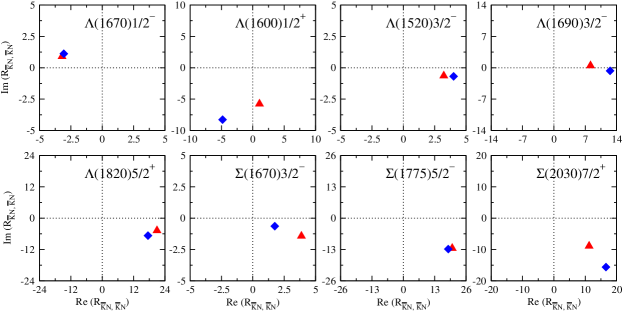
Figure 5: (Color online) Graphical comparison of $R_{\bar{K}N,\bar{K}N}$ between Model A and Model B for the well-established resonances (see text for the details).

We see in Figs. 1 and 2 that the pole masses of eight resonances, represented in the PDG notation by $\Lambda(1670)1/2^{-}$, $\Lambda(1600)1/2^{+}$, $\Lambda(1520)3/2^{-}$, $\Lambda(1690)3/2^{-}$, $\Lambda(1820)5/2^{+}$, $\Sigma(1670)3/2^{-}$, $\Sigma(1775)5/2^{-}$, and $\Sigma(2030)7/2^{+}$, agree very well between our two models and the KSU analysis. The residues $R_{\bar{K}N,\bar{K}N}$ of these resonances extracted from Model A and Model B are compared in Fig. 5. They in general agree well, while visible differences are seen for several resonances. In particular, the pole mass for $\Sigma(1670)3/2^{-}$ agrees within 1 % accuracy between Model A and Model B, but their residues differ by a factor of about 2 in magnitude. This implies that the residues are more sensitive to the analysis than the pole masses.

We now turn to discussing the branching ratios of the decays of the extracted resonances because it may provide us with an intuitive understanding for the properties of the resonances. The branching ratio for the $Y^{*}\to MB$ decay may be defined as $B_{MB}=2|R_{MB,MB}|/\Gamma^{\textrm{tot}}$, where $R_{MB,MB}$ is the residue for the $MB$ scattering amplitude evaluated at the pole position of the considered $Y^{*}$ resonance and $\Gamma^{\textrm{tot}}=-2\mathrm{Im}(M_{R})$ is the total width of the resonance. However, it is known that the sum of the branching ratios defined in this manner do not necessarily equal to unity knls13 ; juelich12 . This would be somewhat problematic as a notion of “ratio,” and will require further studies to give a reasonable interpretation to this definition. Instead, here we will follow the procedures developed in Ref. kpi2pi13 to present the branching ratios evaluated using the following equations,

$$B_{MB}=\frac{\gamma_{MB}}{\sum_{MB}\gamma_{MB}}.$$ (23)

Here, the “partial decay width” $\gamma_{MB}$ is defined for the stable meson-baryon channels ($MB=\bar{K}N,\pi\Sigma,\pi\Lambda,\eta\Lambda,K\Xi$) as

$$\gamma_{MB}=\rho_{MB}(\bar{k};\bar{M})\left|\bar{\Gamma}^{R}_{MB}(\bar{k};\bar{M})\right|^{2},$$ (24)

where $\bar{M}=\mathrm{Re}(M_{R})$, $\bar{k}$ is given by $\bar{M}=E_{M}(\bar{k})+E_{B}(\bar{k})$. For the quasi two-body channels $\pi\Sigma^{*}$ and $\bar{K}^{*}N$ that decay into $\pi\pi\Lambda$ and $\pi\bar{K}N$, respectively, the $\gamma_{MB}$ are given by

$$\gamma_{\pi\Sigma^{*}}=\frac{1}{2\pi}\int^{\bar{M}-m_{\pi}}_{m_{\pi}+m_{\Lambda}}dM_{\pi\Lambda}\frac{-2\mathrm{Im}\bm{(}\Sigma_{\pi\Sigma^{*}}(\bar{k};\bar{M})\bm{)}}{\left|\bar{M}-E_{\pi}(\bar{k})-E_{\Sigma^{*}}(\bar{k})-\Sigma_{\pi\Sigma^{*}}(\bar{k};\bar{M})\right|^{2}}\rho_{\pi\Sigma^{*}}(\bar{k};\bar{M})\left|\bar{\Gamma}^{R}_{\pi\Sigma^{*}}(\bar{k};\bar{M})\right|^{2},$$ (25)

for the case of $MB=\pi\Sigma^{*}$, and

$$\gamma_{\bar{K}^{*}N}=\frac{1}{2\pi}\int^{\bar{M}-m_{N}}_{m_{\pi}+m_{\bar{K}}}dM_{\pi\bar{K}}\frac{-2\mathrm{Im}\bm{(}\Sigma_{\bar{K}^{*}N}(\bar{k};\bar{M})\bm{)}}{\left|\bar{M}-E_{\bar{K}^{*}}(\bar{k})-E_{N}(\bar{k})-\Sigma_{\bar{K}^{*}N}(\bar{k};\bar{M})\right|^{2}}\rho_{\bar{K}^{*}N}(\bar{k};\bar{M})\left|\bar{\Gamma}^{R}_{\bar{K}^{*}N}(\bar{k};\bar{M})\right|^{2},$$ (26)

for the case of $MB=\bar{K}^{*}N$. Here $\Sigma_{MB}(k;W)$ is the self-energy for the $MB$ Green’s function given in Ref. knlskp1 ; $\bar{k}$ is defined by $\bar{M}=E_{\pi}(\bar{k})+\sqrt{M_{\pi\Lambda}^{2}+\bar{k}^{2}}$ [$\bar{M}=E_{N}(\bar{k})+\sqrt{M_{\pi\bar{K}}^{2}+\bar{k}^{2}}$] for $MB=\pi\Sigma^{*}$ [$MB=\bar{K}^{*}N$]; and the undressed values listed in Table V of Ref. knlskp1 are used for the $\Sigma^{*}$ and $\bar{K}^{*}$ masses. The integrals in Eqs. (25) and (26) account for the phase space of the final three-body states. As expected, Eqs. (25) and (26) are reduced to Eq. (24) for the stable two-body channels in the limit of $\Sigma_{\pi\Sigma^{*}}\to 0$ and $\Sigma_{\bar{K}^{*}N}\to 0$, respectively.

Summing up the branching ratios defined by Eqs. (23)-(26) trivially results in unity. We have confirmed that the branching ratios defined by Eqs. (23)-(26) are in good agreement with the ones defined by $B_{MB}=2|R_{MB,MB}|/\Gamma^{\textrm{tot}}$ if the sum of the latter ratios is within the range between 0.9 and 1.1.

The resulting branching ratios and their graphical representations are presented in Table 7 and Fig. 6 (Table 8 and Fig. 7) for Model A (Model B). Except few cases, the low-mass resonances generally have large branching ratios of their decays into the $\bar{K}N$ and $\pi\Sigma$ channels. We also note that the branching ratios to the $\eta\Lambda$ channel of the narrow $S$-wave $\Lambda$ resonances at $\mathrm{Re}(M_{R})\sim 1.67$ GeV, namely $\Lambda(1669)1/2^{-}$ for Model A and $\Lambda(1667)1/2^{-}$ for Model B, are large and comparable. The new narrow $P_{03}$ resonances, $\Lambda(1671)3/2^{+}$, found in Model B also has the same feature. This can be understood from their sizable contributions to the $K^{-}p\to\eta\Lambda$ total cross sections near the threshold. Also, the low-lying $\Sigma^{*}$ resonances found in Model B, $\Sigma(1457)1/2^{+}$ and $\Sigma(1492)3/2^{-}$, largely decay into the $\pi\Lambda$ channel. On the other hand, the high-mass resonances are found to have large branching ratios to $\pi\Sigma^{*}$ and $\bar{K}^{*}N$ channels, which decay subsequently to the three-body $\pi\pi\Lambda$ and $\pi\bar{K}N$ channels, respectively. For example, the $J^{P}=7/2^{+}$ $\Sigma$ resonance that would correspond to the four-star $\Sigma(2030)7/2^{+}$ of PDG, namely $\Sigma(2025)7/2^{+}$ for Model A and $\Sigma(2014)7/2^{+}$ for Model B, has a large breaching ratio to the three-body decay channels. Interestingly, the $J^{P}=7/2^{+}$ $\Sigma$ resonance of Model A mainly decays into $\pi\bar{K}N$, while that of Model B decays into $\pi\pi\Lambda$, revealing that our knowledge of the properties of this four-star resonance is still poor. This implies a particular importance of the data associated with three-body channels for establishing the high-mass $\Lambda^{*}$ and $\Sigma^{*}$ spectrum and their internal structures. This is quite similar to the case of the $N^{*}$ and $\Delta^{*}$ spectroscopy, where the data associated with the three-body $\pi\pi N$ channel are expected to play a crucial role for establishing the high-mass $N^{*}$ and $\Delta^{*}$ resonance mass spectrum, see, e.g., Ref. kpi2pi13 .

Table 7: Branching ratios for the decays of $\Lambda^{*}$ and $\Sigma^{*}$ resonances extracted from Model A. Equations (23)-(26) are used for evaluating the ratios. The quantum numbers for the $(\pi\Sigma^{*})_{i}$ ($i=1,2$) and $(\bar{K}^{*}N)_{i}$ ($i=1,2,3$) channels for a given $J^{P}$ are presented in Table 1

	Branching ratios (%)
Particle $J^{P}(l_{I2J})$	$B_{\bar{K}N}$	$B_{\pi\Sigma}$	$B_{\eta\Lambda}$	$B_{K\Xi}$	$B_{(\pi\Sigma^{*})_{1}}$	$B_{(\pi\Sigma^{*})_{2}}$	$B_{(\bar{K}^{*}N)_{1}}$	$B_{(\bar{K}^{*}N)_{2}}$	$B_{(\bar{K}^{*}N)_{3}}$
$\Lambda(1669)1/2^{-}(S_{01})$	31.8	28.9	37.3	-	1.9	-	0.0	0.0	-
$\Lambda(1544)1/2^{+}(P_{01})$	6.4	85.1	-	-	8.5	-	-	-	-
$\Lambda(2097)1/2^{+}(P_{01})$	22.5	0.9	11.1	5.1	47.0	13.0	0.3	-	-
$\Lambda(1859)3/2^{+}(P_{03})$	30.5	4.0	1.2	0.9	45.3	1.9	7.3	8.8	0.1
$\Lambda(1517)3/2^{-}(D_{03})$	43.0	44.6	-	-	12.1	0.3	-	-	-
$\Lambda(1697)3/2^{-}(D_{03})$	23.9	38.7	0.0	-	6.2	30.8	0.0	0.3	0.0
$\Lambda(1766)5/2^{-}(D_{05})$	4.6	62.1	0.7	-	32.4	0.1	0.1	0.1	0.0
$\Lambda(1899)5/2^{-}(D_{05})$	0.6	1.7	2.4	56.2	13.4	0.0	13.4	11.5	0.9
$\Lambda(1824)5/2^{+}(F_{05})$	54.7	21.8	0.1	0.0	17.3	5.5	0.0	0.6	0.0
$\Lambda(1757)7/2^{+}(F_{07})$	0.0	89.1	0.2	-	10.5	0.0	0.0	0.1	0.0
Particle $J^{P}(l_{I2J})$	$B_{\bar{K}N}$	$B_{\pi\Sigma}$	$B_{\pi\Lambda}$	$B_{K\Xi}$	$B_{(\pi\Sigma^{*})_{1}}$	$B_{(\pi\Sigma^{*})_{2}}$	$B_{(\bar{K}^{*}N)_{1}}$	$B_{(\bar{K}^{*}N)_{2}}$	$B_{(\bar{K}^{*}N)_{3}}$
$\Sigma(1704)1/2^{-}(S_{11})$	15.4	37.3	43.5	-	2.4	-	0.4	1.0	-
$\Sigma(1547)1/2^{+}(P_{11})$	0.5	86.5	12.8	-	0.1	-	-	-	-
$\Sigma(1706)1/2^{+}(P_{11})$	1.6	59.5	28.3	-	10.3	-	0.4	0.0	-
$\Sigma(1607)3/2^{-}(D_{13})$	0.3	38.7	49.0	-	12.0	0.1	0.0	0.0	0.0
$\Sigma(1669)3/2^{-}(D_{13})$	12.1	46.5	5.8	-	30.9	4.4	0.1	0.2	0.1
$\Sigma(1767)5/2^{-}(D_{15})$	40.2	4.2	24.4	-	30.9	0.0	0.0	0.3	0.0
$\Sigma(1890)5/2^{+}(F_{15})$	3.6	67.8	12.7	0.0	11.2	0.4	0.1	4.2	0.0
$\Sigma(2025)7/2^{+}(F_{17})$	26.9	3.7	8.0	0.6	3.0	0.3	15.4	42.2	0.0

Table 8: Branching ratios for the decays of $\Lambda^{*}$ and $\Sigma^{*}$ resonances extracted from Model B. Equations (23)-(26) are used for evaluating the ratios. The quantum numbers for the $(\pi\Sigma^{*})_{i}$ ($i=1,2$) and $(\bar{K}^{*}N)_{i}$ ($i=1,2,3$) channels for a given $J^{P}$ are presented in Table 1

	Branching ratios (%)
Particle $J^{P}(l_{I2J})$	$B_{\bar{K}N}$	$B_{\pi\Sigma}$	$B_{\eta\Lambda}$	$B_{K\Xi}$	$B_{(\pi\Sigma^{*})_{1}}$	$B_{(\pi\Sigma^{*})_{2}}$	$B_{(\bar{K}^{*}N)_{1}}$	$B_{(\bar{K}^{*}N)_{2}}$	$B_{(\bar{K}^{*}N)_{3}}$
$\Lambda(1512)1/2^{-}(S_{01})$	63.6	36.4	-	-	0.0	-	-	-	-
$\Lambda(1667)1/2^{-}(S_{01})$	36.3	26.6	21.2	-	15.5	-	0.3	0.1	-
$\Lambda(1548)1/2^{+}(P_{01})$	24.0	70.9	-	-	5.0	-	-	-	-
$\Lambda(1841)1/2^{+}(P_{01})$	23.7	10.9	4.0	13.2	14.9	-	0.5	32.9	-
$\Lambda(1671)3/2^{+}(P_{03})$	3.9	18.6	43.2	-	33.9	0.1	0.2	0.1	0.0
$\Lambda(1517)3/2^{-}(D_{03})$	43.1	46.2	-	-	10.1	0.6	-	-	-
$\Lambda(1697)3/2^{-}(D_{03})$	31.8	29.8	0.1	-	2.9	34.3	0.0	1.1	0.0
$\Lambda(1924)5/2^{-}(D_{05})$	5.4	1.3	0.1	0.4	85.7	0.1	2.4	1.4	3.1
$\Lambda(1821)5/2^{+}(F_{05})$	56.5	15.3	0.5	0.0	25.2	0.8	0.0	1.7	0.0
$\Lambda(2041)7/2^{+}(F_{07})$	1.6	56.5	1.7	26.4	9.5	0.1	1.5	1.9	0.9
Particle $J^{P}(l_{I2J})$	$B_{\bar{K}N}$	$B_{\pi\Sigma}$	$B_{\pi\Lambda}$	$B_{K\Xi}$	$B_{(\pi\Sigma^{*})_{1}}$	$B_{(\pi\Sigma^{*})_{2}}$	$B_{(\bar{K}^{*}N)_{1}}$	$B_{(\bar{K}^{*}N)_{2}}$	$B_{(\bar{K}^{*}N)_{3}}$
$\Sigma(1551)1/2^{-}(S_{11})$	45.6	8.0	46.3	-	0.0	-	-	-	-
$\Sigma(1940)1/2^{-}(S_{11})$	53.4	20.4	1.9	4.0	3.3	-	3.2	13.9	-
$\Sigma(1457)1/2^{+}(P_{11})$	1.2	2.1	96.7	-	0.0	-	-	-	-
$\Sigma(1605)1/2^{+}(P_{11})$	3.6	41.8	43.4	-	11.2	-	0.0	0.0	-
$\Sigma(2014)1/2^{+}(P_{11})$	10.4	7.5	10.0	5.7	17.2	-	16.1	33.1	-
$\Sigma(1492)3/2^{-}(D_{13})$	0.0	9.2	90.7	-	0.1	0.0	-	-	-
$\Sigma(1672)3/2^{-}(D_{13})$	6.8	81.0	6.6	-	1.6	2.2	0.0	1.8	0.0
$\Sigma(1765)5/2^{-}(D_{15})$	39.7	5.9	18.3	-	36.1	0.0	0.1	0.0	0.0
$\Sigma(1695)5/2^{+}(F_{15})$	0.3	46.4	53.0	-	0.2	0.0	0.0	0.0	0.0
$\Sigma(2014)7/2^{+}(F_{17})$	29.1	0.7	6.3	0.7	57.8	0.5	1.0	1.9	2.0

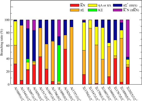
Figure 6: (Color online) Graphical representation of the branching ratios for decays of $\Lambda^{*}$ and $\Sigma^{*}$ resonances found from Model A. Equations (23)-(26) are used for evaluating the ratios.

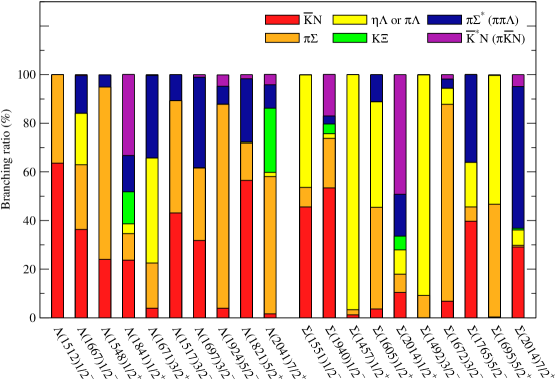
Figure 7: (Color online) Graphical representation of the branching ratios for decays of $\Lambda^{*}$ and $\Sigma^{*}$ resonances found from Model B. Equations (23)-(26) are used for evaluating the ratios.

IV $S$-wave $\Lambda$ resonances below the $\bar{K}N$ threshold

The nature of the $S$-wave ($J^{P}=1/2^{-}$) $\Lambda$ resonances lying below the $\bar{K}N$ threshold has long been an interesting subject since they are closely related to the extensively discussed $\Lambda(1405)$ l1405 . In this section, we discuss such $S$-wave $\Lambda$ resonances extracted from our models. However, here we add a caveat that Models A and B were constructed by analyzing only the $K^{-}p$ reactions, and hence the $\bar{K}N$ subthreshold region is beyond the scope of our current analysis. Therefore, the results presented below should be considered as the “predictions” from our current models and are subject to change once our analysis is extended to include the data in the $\bar{K}N$ subthreshold region. For this reason, we do not evaluate the uncertainties of the masses of these resonances.

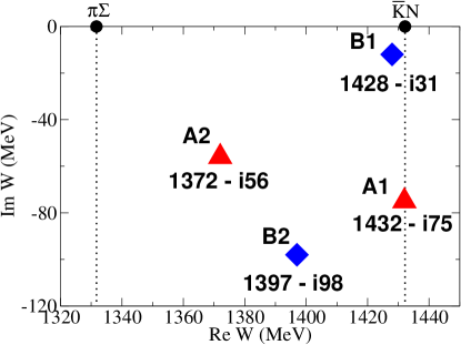
Figure 8: (Color online) $S$-wave ($J^{P}=1/2^{-}$) $\Lambda$ resonances in the $\bar{K}N$ subthreshold region. Red triangles (blue diamonds) are resonance poles found from Model A (Model B).

Within our model, the $S$-wave $\Lambda$ resonances found in the region below the $\bar{K}N$ threshold are presented in Fig. 8. The red triangles and the blue diamonds represent the pole positions obtained from Model A and Model B, respectively. Both models predict two resonance poles for the $S$-wave $\Lambda$ resonances in the $\bar{K}N$ subthreshold region, while their positions are rather different. This indicates a need of extending our analysis to include the data in the $\bar{K}N$ subthreshold region. Higher mass poles (A1 and B1 in Fig. 8) seem to correspond to $\Lambda(1405)$, though the pole A1 has an imaginary part somewhat larger than what is usually expected for $\Lambda(1405)$. The existence of another $\Lambda$ resonance with lower mass (A2 and B2 in Fig. 8) is similar to the result obtained in the so-called chiral unitary models (see, e.g., Ref. ucm-1 ). In Table 9, we list the residues for the $J^{P}=1/2^{-}$ $\Lambda$ resonances presented in Fig. 8.

Table 9: Residues for $\pi\Sigma\to Y^{*}\to\pi\Sigma$ amplitudes [$R_{\pi\Sigma,\pi\Sigma}$ (MeV)] at the $J^{P}=1/2^{-}$ $\Lambda^{\ast}$ resonance pole positions found below $\bar{K}N$ threshold. See the caption of Table 3 for the description of the table.

	Particle $J^{P}(l_{I2J})$	$R_{\pi\Sigma,\pi\Sigma}$
		$R$	$\phi$
Model A	$\Lambda(1372)1/2^{-}(S_{01})$	118	$-$68
	$\Lambda(1432)1/2^{-}(S_{01})$	177	144
Model B	$\Lambda(1397)1/2^{-}(S_{01})$	142	$-$98
	$\Lambda(1428)1/2^{-}(S_{01})$	67	110

Since the poles $A1$ and $B1$ are located near the $\bar{K}N$ threshold, it is interesting to examine the correlation between their pole values and the $S$-wave threshold parameters for the $I=0$ $\bar{K}N$ scattering amplitude, as done for the $\Lambda(1670)1/2^{-}$ resonance near the $\eta\Lambda$ threshold (see Sec. III.1). Similar to Eq. (19), the $S_{01}$ $\bar{K}N$ scattering amplitude near the threshold can be written as

$$F^{I=0,S\mathrm{wave}}_{\bar{K}N,\bar{K}N}(k)\simeq k\times\left(\frac{1}{a^{I=0}_{\bar{K}N}}-ik+\frac{r^{I=0}_{\bar{K}N}}{2}k^{2}\right)^{-1},$$ (27)

where $a^{I=0}_{\bar{K}N}$ and $r^{I=0}_{\bar{K}N}$ are the scattering length and effective range for the $I=0$ $\bar{K}N$ scattering, respectively. These threshold parameters have been extracted in our previous paper knlskp1 , and their values are:

$$a^{I=0}_{\bar{K}N}=\left\{\begin{array}[]{cc}-1.37+i0.67~{}\mathrm{fm}&(\mathrm{Model~{}A}),\\ -1.62+i1.02~{}\mathrm{fm}&(\mathrm{Model~{}B}),\end{array}\right.$$ (28)

$$r^{I=0}_{\bar{K}N}=\left\{\begin{array}[]{cc}0.67-i0.25~{}\mathrm{fm}&(\mathrm{Model~{}A}),\\ 0.74-i0.25~{}\mathrm{fm}&(\mathrm{Model~{}B}).\end{array}\right.$$ (29)

By performing the same procedure as done for the $\Lambda(1670)1/2^{-}$ resonance in Sec. III.1, we find that the approximate amplitude (27) has a pole at the complex $W$ with

$$W=E_{\bar{K}}(k)+E_{N}(k)=\left\{\begin{array}[]{cc}1408-i56~{}\mathrm{MeV}&(\mathrm{Model~{}A}),\\ 1427-i29~{}\mathrm{MeV}&(\mathrm{Model~{}B}).\end{array}\right.$$ (30)

We find that the above value for Model B agrees well with the exact pole mass for the pole B1, while for Model A we find a significant deviation from the pole A1. This can be understood because the position of the pole A1, as indicated in Fig.8, is a bit far from the $\bar{K}N$ threshold and the approximated expression (27) of the amplitude becomes less accurate than the case of the pole B1. We also see in Fig.8 that the poles $A2$ and $B2$ are even farther from the $\bar{K}N$ threshold and hence they can not be well reproduced by the poles extracted from the approximate amplitude defined by Eq. (27).

V Summary and future developments

We have presented the parameters associated with the $\Lambda^{*}$ and $\Sigma^{*}$ resonances extracted from our DCC models that were constructed via a comprehensive partial-wave analysis of the $K^{-}p\to\bar{K}N,\pi\Sigma,\pi\Lambda,\eta\Lambda,K\Xi$ data knlskp1 . The extraction was accomplished by searching for poles of scattering amplitudes in the complex energy Riemann surface over the region with $m_{\bar{K}}+m_{N}<\mathrm{Re}(W)<2.1$ GeV and $0<-2\mathrm{Im}(W)<0.4$ GeV. As a result, 18 (20) resonances are extracted from Model A (Model B) above the $\bar{K}N$ threshold. The residues and branching ratios for the extracted resonances are also presented, and their values are found to be more sensitive to differences between the analyses than the pole values.

Among the extracted resonances, a new narrow $J^{P}=3/2^{+}$ $\Lambda$ resonance with $M_{R}=1671^{+2}_{-8}-i(5^{+11}_{-2})$ MeV is of particular interest. Currently, this resonance is only found in Model B. However, the angular dependence of the $K^{-}p\to\eta\Lambda$ differential cross section data seems to favor the existence of this resonance. Given the fact that this new resonance is identified only through its contribution to the spin-averaged differential cross section of the $K^{-}p\to\eta\Lambda$ reaction near the threshold, the polarization data would be highly desirable to have a definitive conclusion on the existence of this resonance. Also, establishing low-lying $\Sigma^{*}$ resonances in $S_{11}$, $P_{11}$, and $D_{13}$ waves would also be an important task for the $Y^{*}$ spectroscopy.

By comparing the results from our two models and the KSU analysis, we found that the extracted resonance parameters have significant analysis dependence. This reflects the fact that the kinematical ($W$ and $\cos\theta$) coverage and accuracy of the available $K^{-}p$ reaction data are far from “complete” and not sufficient to eliminate analysis dependence on the extracted resonance parameters. More extensive and accurate data of the $K^{-}p$ reactions including the differential cross sections as well as the polarization observables (the recoil polarization $P$ and the spin-rotation parameters $\beta$, $R$, and $A$) are definitely needed to get convergent results. In fact, the data of all observables are relevant to accomplish an accurate extraction of amplitudes and resonance parameters with less analysis dependence, as discussed in, for example, Ref. shkl11 . An impact of unmeasured observables of the $K^{-}p\to MB$ reactions for reducing analysis dependence has been explored in our previous paper knlskp1 . We have also found that the high-mass $\Lambda^{*}$ and $\Sigma^{*}$ resonances have large branching ratios to the quasi two-body $\pi\Sigma^{*}$ and $\bar{K}^{*}N$ channels, suggesting that the data for the $2\to 3$ reactions such as $K^{-}p\to\pi\pi\Lambda$ and $K^{-}p\to\pi\bar{K}N$ will also play an important role for establishing the high-mass resonances. The experiments measuring these fundamental observables at the hadron beam facilities, such as J-PARC, will be essential for making progress in establishing the $\Lambda^{*}$ and $\Sigma^{*}$ resonances.

As a byproduct of our $K^{-}p$ reaction analysis, we have given “predictions” for the $J^{P}=1/2^{-}$ $\Lambda$ resonances located below the $\bar{K}N$ threshold. Both of our two models predict a resonance pole just below the $\bar{K}N$ threshold, which would correspond to $\Lambda(1405)1/2^{-}$. Our two models also predict another $J^{P}=1/2^{-}$ $\Lambda$ resonance pole with the mass $\sim$30-60 MeV lower than $\Lambda(1405)1/2^{-}$ we found. This result is similar to what is obtained within the chiral unitary models ucm-1 . To make a decisive examination for the $J^{P}=1/2^{-}$ $\Lambda$ resonances, however, we must extend our analysis to include the data in the $\bar{K}N$ subthreshold region. Our effort, in conjunction with the recent experimental initiatives moriya ; j-parc-e31 will be published elsewhere.