Event-Triggered $H_{\infty}$ Control: a Switching Approach

Abstract

Event-triggered approach to networked control systems is used to reduce the workload of the communication network. For the static output-feedback continuous event-trigger may generate an infinite number of sampling instants in finite time (Zeno phenomenon) what makes it inapplicable to the real-world systems. Periodic event-trigger avoids this behavior but does not use all the available information. In the present paper we aim to exploit the advantage of the continuous-time measurements and guarantee a positive lower bound on the inter-event times by introducing a switching approach for finding a waiting time in the event-triggered mechanism. Namely, our idea is to present the closed-loop system as a switching between the system under periodic sampling and the one under continuous event-trigger and take the maximum sampling preserving the stability as the waiting time. We extend this idea to the $L_{2}$-gain and ISS analysis of perturbed networked control systems with network-induced delays. By examples we demonstrate that the switching approach to event-triggered control can essentially reduce the amount of measurements to be sent through a communication network compared to the existing methods.

1 Introduction

Networked control systems (NCS), that are comprised of sensors, actuators, and controllers connected through a communication network, have been recently extensively studied by researchers from a variety of disciplines [3, 4, 5, 6]. One of the main challenges in such systems is that only sampled in time measurements can be transmitted through a communication network. Namely, consider the system

$$\dot{x}(t)=Ax(t)+Bu(t),\quad y(t)=Cx(t),$$ (1)

with a state $x\in\mathbb{R}^{n}$, input $u\in\mathbb{R}^{m}$, and output $y\in\mathbb{R}^{l}$. Assume that there exists $K\in\mathbb{R}^{m\times l}$ such that the control signal $u(t)=-Ky(t)$ stabilizes the system (1). In NCS the measurements can be transmitted to the controller only at discrete time instants

$$0=s_{0}<s_{1}<s_{2}<\ldots,\quad\lim_{k\to\infty}s_{k}=\infty.$$ (2)

Therefore, the closed-loop system has the form

$$\dot{x}(t)=Ax(t)-BKCx(s_{k}),\quad t\in[s_{k},s_{k+1}),\quad k\in\mathbb{N}_{0},$$ (3)

where $\mathbb{N}_{0}$ is the set of nonnegative integers. There are different ways of obtaining the sequence of sampling instants $s_{k}$ that preserve the stability. The simplest approach is periodic sampling where one chooses $s_{k}=kh$ with appropriate period $h$. Under periodic sampling the measurements are sent even when the output fluctuation is small and does not significantly change the control signal. To avoid these “redundant” packets one can use continuous event-trigger [7], where

$$s_{k+1}=\min\{t>s_{k}\,|\,(y(t)-y(s_{k}))^{T}\Omega(y(t)-y(s_{k}))\geq\varepsilon y^{T}(t)\Omega y(t)\}$$ (4)

with a matrix $\Omega\geq 0$ and a scalar $\varepsilon>0$. In case of a static output-feedback execution times $s_{k}$, implicitly defined by (4), can be such that $\lim_{k\to\infty}s_{k}<\infty$ [8]. That is, an infinite number of events is generated in finite time what makes (4) inapplicable to NCS. To avoid this Zeno phenomenon one can use periodic event-trigger [9, 10, 11, 12] by choosing

$$s_{k+1}\!=\!\min\{s_{k}+ih\,|\,i\in\mathbb{N},\,(y(s_{k}+ih)-y(s_{k}))^{T}\Omega(y(s_{k}+ih)-y(s_{k}))\!>\!\varepsilon y^{T}(s_{k}+ih)\Omega y(s_{k}+ih)\}.$$ (5)

This approach guarantees that the inter-event times are at least $h$ and fits the case where the sensor measures only sampled in time outputs $y(ih)$.

However, when the continuous measurements are available one can use this additional information to improve the control algorithm. In [13, 14, 15] the following strategy of choosing the sampling instants has been considered:

$$s_{k+1}=\min\{t\geq s_{k}+T\,|\,\eta\geq 0\},$$ (6)

where $T>0$ is a constant waiting time and $\eta$ is an event-trigger condition. In [14, 15] the value of $T$ that preserves the stability was obtained by solving a scalar differential equation. For $\eta=|y(t)-y(t_{k})|-C$ with a constant $C$ some qualitative results concerning practical stability have been obtained in [13].

In this work we propose a new constructive and efficient method of finding an appropriate waiting time. Our idea is to present the closed-loop system as a switching between the system under periodic sampling and the one under continuous event-trigger and take the maximum sampling preserving the stability as a waiting time. We extend this idea to the systems with network-induced delays, external disturbances, and measurement noise (Section 3). Differently from [13, 14, 15, 9] our method is applicable to uncertain linear systems and the waiting time is found from LMIs. Comparatively to periodic event-trigger of [10, 11, 12] our method leads to error separation between the system under periodic sampling and the one under continuous event-trigger that allows for larger sampling periods for the same values of the event-trigger parameter $\varepsilon$. The latter allows to reduce the amount of sent measurements as illustrated by examples brought from [7], [8], and [16] (Section 4).

2 A switching approach to event-trigger

Consider (1). Assume that there exists $K$ such that $A-BKC$ is Hurwitz. For $C=I$ such $K$ exists if $(A,B)$ is stabilizable. For the static output-feedback case such $K$ exists if the transfer function $C(sI-A)^{-1}B$ is hyper-minimum-phase (has stable zeroes and positive leading coefficient of the numerator, see, e.g., [17]). Assume that the measurements are sent at time instants (2). According to [18] the closed-loop system (3) under periodic sampling $s_{k}=kh$ can be presented in the form

$$\dot{x}(t)=(A-BKC)x(t)+BKC\int_{t-\tau(t)}^{t}\dot{x}(s)\,ds,$$ (7)

where $\tau(t)=t-s_{k}$ for $t\in[s_{k},s_{k+1})$. The system (3) under continuous event-trigger (4) can be rewritten as (see [7])

$$\dot{x}(t)=(A-BKC)x(t)-BKe(t)$$ (8)

with $e(t)=y(s_{k})-y(t)$ for $t\in[s_{k},s_{k+1})$.

Under periodic sampling (leading to (7)) “redundant” packets can be sent while continuous event-trigger (that leads to (8)) can cause Zeno phenomenon. To avoid the above drawbacks periodic event-trigger (5) can be used, where the closed-loop system can be written as

$$\dot{x}(t)=(A-BKC)x(t)+BKC\int_{t-\tau(t)}^{t}\dot{x}(s)\,ds-BKe(t)$$ (9)

with $\tau(t)=t-s_{k}-ih\leq h$, $e(t)=y(s_{k})-y(s_{k}+ih)$ for $t\in[s_{k}+ih,s_{k}+(i+1)h)$, $i\in\mathbb{N}_{0}$ such that $s_{k}+(i+1)h\leq s_{k+1}$. As one can see, the error due to sampling that appears in (7) (the integral term) and the error $e(t)$ due to triggering from (8) are both presented in (9) what makes it more difficult to ensure the stability of (9) compared to (7) or (8).

We propose an event-trigger that allows to separate these errors by considering the switching between periodic sampling and continuous event-trigger. Namely, after the measurement has been sent, the sensor waits for at least $h$ seconds (that corresponds to $T$ in (6)). During this time the system is described by (7). Then the sensor begins to continuously check the event-trigger condition and sends the measurement when it is violated. During this time the system is described by (8). This leads to the following choice of sampling:

$$s_{k+1}=\min\{s\geq s_{k}+h\,|\,(y(s)-y(s_{k}))^{T}\Omega(y(s)-y(s_{k}))\geq\varepsilon y^{T}(s)\Omega y(s)\}$$ (10)

with a matrix $\Omega\geq 0$ and scalars $\varepsilon\geq 0$, $h>0$, where the inter-event times are not less than $h$. The system (3), (10) can be presented as a switching between (7) and (8):

$$\dot{x}(t)=(A-BKC)x(t)+\chi(t)BKC\int_{t-\tau(t)}^{t}\dot{x}(s)\,ds-(1-\chi(t))BKe(t),$$ (11)

where

$$\begin{aligned} \tau(t)&=t-s_{k}\leq h,&&t\in[s_{k},s_{k}+h),\\ e(t)&=y(s_{k})-y(t),&&t\in[s_{k}+h,s_{k+1}),\end{aligned}$$ (12)

$$\chi(t)=\left\{\begin{aligned} &1,&&t\in[s_{k},s_{k}+h),\\ &0,&&t\in[s_{k}+h,s_{k+1}).\end{aligned}\right.$$

To obtain the stability conditions for the switched system (11) we use different Lyapunov functions: for (11) with $\chi(t)=0$ we consider

$$V_{P}(x)=x^{T}(t)Px(t),\quad P>0,$$ (13)

for (11) with $\chi(t)=1$ we apply the functional from [19]:

$$V(t,x_{t},\dot{x}_{t})=V_{P}(x(t))+V_{U}(t,\dot{x}_{t})+V_{X}(t,x_{t}),$$ (14)

where $x_{t}(\theta)=x(t+\theta)$ for $\theta\in[-h,0]$, $V_{P}$ is given by (13),

$$V_{U}(t,\dot{x}_{t})=(h-\tau(t))\int_{t_{k}}^{t}e^{2\delta(s-t)}\dot{x}^{T}(s)U\dot{x}(s)\,ds,\,U>0,$$

$$V_{X}(t,x_{t})=(h-\tau(t))\left[\begin{matrix}x(t)\\ x(t_{k})\end{matrix}\right]^{T}\left[\begin{matrix}\frac{X+X^{T}}{2}&-X+X_{1}\\ *&-X_{1}-X_{1}^{T}+\frac{X+X^{T}}{2}\end{matrix}\right]\left[\begin{matrix}x(t)\\ x(t_{k})\end{matrix}\right].$$

Note that the values of $V$ and $V_{P}$ coincide at the switching instants $t_{k}$ and $t_{k}+h$.

Theorem 1.

For given scalars $h>0$, $\varepsilon\geq 0$, $\delta\geq 0$ let there exist $n\times n$ matrices $P>0$, $U>0$, $X$, $X_{1}$, $P_{2}$, $P_{3}$, $Y_{1}$, $Y_{2}$, $Y_{3}$ and $l\times l$ matrix $\Omega\geq 0$ such that

$$\Xi>0,\quad\Psi_{0}\leq 0,\quad\Psi_{1}\leq 0,\quad\Phi\leq 0,$$ (15)

where

$$\Xi =\left[\begin{matrix}P+h\frac{X+X^{T}}{2}&hX_{1}-hX\\ *&-hX_{1}-hX_{1}^{T}+h\frac{X+X^{T}}{2}\end{matrix}\right],$$

$$\Phi =\left[\begin{matrix}\Phi_{11}&\Phi_{12}&-P_{2}^{T}BK\\ *&-P_{3}^{T}-P_{3}&-P_{3}^{T}BK\\ *&*&-\Omega\end{matrix}\right],$$

$$\Psi_{0} =\left[\begin{matrix}\Psi_{11}-X_{\delta}&\Psi_{12}+h\frac{X+X^{T}}{2}&\Psi_{13}+X_{1\delta}\\ *&\Psi_{22}+hU&\Psi_{23}-h(X-X_{1})\\ *&*&\Psi_{33}-X_{2\delta}|_{\tau=0}\end{matrix}\right],$$

$$\Psi_{1} =\left[\begin{matrix}\Psi_{11}-\frac{X+X^{T}}{2}&\Psi_{12}&\Psi_{13}+X-X_{1}&hY_{1}^{T}\\ *&\Psi_{22}&\Psi_{23}&hY_{2}^{T}\\ *&*&\Psi_{33}-X_{2\delta}|_{\tau=h}&hY_{3}^{T}\\ *&*&*&-hUe^{-2\delta h}\end{matrix}\right],$$

$$\begin{array}[]{l}\Phi_{11}=P_{2}^{T}(A-BKC)+(A-BKC)^{T}P_{2}+\varepsilon C^{T}\Omega C+2\delta P,\\ \Phi_{12}=P+(A-BKC)^{T}P_{3}-P_{2}^{T},\\ \Psi_{11}=A^{T}P_{2}+P_{2}^{T}A+2\delta P-Y_{1}-Y_{1}^{T},\\ \Psi_{12}=P-P_{2}^{T}+A^{T}P_{3}-Y_{2},\\ \Psi_{13}=Y_{1}^{T}-P_{2}^{T}BKC-Y_{3},\\ \Psi_{22}=-P_{3}-P_{3}^{T},\\ \Psi_{23}=Y_{2}^{T}-P_{3}^{T}BKC,\\ \Psi_{33}=Y_{3}+Y_{3}^{T},\quad X_{\delta}=(1\!/2-\delta h)(X+X^{T}),\\ X_{1\delta}=(1-2\delta h)(X-X_{1}),\\ X_{2\delta}=(1\!/2-\delta(h-\tau))(X+X^{T}-2X_{1}-2X_{1}^{T}).\end{array}$$

Then the system (3) under the event-trigger (10) is exponentially stable with a decay rate $\delta$.

Proof. The system (3), (10) is presented in the form of the switched system (11). According to [19] the conditions $\Xi>0$, $\Psi_{0}\leq 0$, $\Psi_{1}\leq 0$ imply $V\geq\alpha|x(t)|^{2}$ and $\dot{V}\leq-2\delta V$ for the system (11) with $\chi(t)=1$. Consider (11) with $\chi(t)=0$. Since for $t\in[s_{k}+h,s_{k+1})$ the relation (10) implies

$$0\leq\varepsilon x^{T}(t)C^{T}\Omega Cx(t)-e^{T}(t)\Omega e(t),$$ (16)

we add (16) to $\dot{V}_{P}$ to compensate the cross term with $e(t)$. We have

$$\dot{V}_{P}+2\delta V_{P}\leq 2x^{T}P\dot{x}+2\delta x^{T}Px+2[x^{T}P_{2}^{T}+\dot{x}^{T}P_{3}^{T}][(A-BKC)x-BKe-\dot{x}]\\ +[\varepsilon x^{T}C^{T}\Omega Cx-e^{T}\Omega e]=\varphi^{T}\Phi\varphi\leq 0,$$

where $\varphi=\operatorname{col}\{x,\dot{x},e\}$. Thus, $\dot{V}_{P}\leq-2\delta V_{P}$.

The stability of the switched system (11) follows from the fact that at the switching instants $s_{k}$ and $s_{k}+h$ the values of $V$ and $V_{P}$ coincide.

$\square$

By extending the proof from [19] we obtain the stability conditions for the system (3), (5) presented in the form (9):

Remark 1.

For given scalars $h>0$, $\varepsilon\geq 0$, $\delta>0$ let there exist $n\times n$ matrices $P>0$, $U>0$, $X$, $X_{1}$, $P_{2}$, $P_{3}$, $Y_{1}$, $Y_{2}$, $Y_{3}$ and $l\times l$ matrix $\Omega\geq 0$ such that

$$\Xi>0,\quad\left[\begin{array}[]{c:c}&-P_{2}^{T}BK\\ \overline{\Psi}_{i}&-P_{3}^{T}BK\\ &0\\ \hdashline*&-\Omega\end{array}\right]\leq 0,$$ (17)

where $\overline{\Psi}_{i}=\Psi_{i}+\varepsilon[I_{n}\,0]^{T}C^{T}\Omega C[I_{n}\,0]$, $i=0,1$. Then the system (3) under periodic event-trigger (5) is exponentially stable with a decay rate $\delta$.

Remark 2.

The feasibility of (17) implies the feasibility of (15). Therefore, the stability of (3) under (10) can be guaranteed for not smaller $h$ and $\varepsilon$ than under (5). Examples in Section 4 show that these values under (10) are essentially larger what allows to reduce the amount of sent measurements. Note that for the same $h$, $\varepsilon$, and $\Omega$ the amount of sent measurements under periodic event-trigger (5) is deliberately less than under (10). Indeed, if the measurement is sent at $s_{k}$ and the event-trigger rule is satisfied at $s_{k}+h$, according to (5) the sensor will wait till at least $s_{k}+2h$ before sending the next measurement, while according to (10) the next measurement can be sent before $s_{k}+2h$.

3 Event-trigger under network-induced delays and disturbances

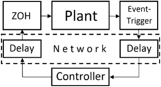
Figure 1: Scheme of a system with network-induced delays

Consider the system

$$\dot{x}(t) =Ax(t)+B_{1}w(t)+B_{2}u(t),$$ (18)

$$z(t) =C_{1}x(t)+D_{1}u(t),$$

$$y(t) =C_{2}x(t)+D_{2}v(t)$$

with a state $x\in\mathbb{R}^{n}$, input $u\in\mathbb{R}^{m}$, controlled output $z\in\mathbb{R}^{n_{z}}$, measurements $y\in\mathbb{R}^{l}$, and disturbances $w\in\mathbb{R}^{n_{w}}$, ${v\in\mathbb{R}^{n_{v}}}$. Denote by $\eta_{k}\leq\eta_{M}$ the overall network-induced delay from the sensor to the actuator that affects the transmitted measurement $y(s_{k})$ (see Fig. 1). Here $s_{k}$ is a sampling instant on the sensor side. We assume that $\eta_{k}$ are such that the ZOH updating times $t_{k}=s_{k}+\eta_{k}$ satisfy

$$t_{k}=s_{k}+\eta_{k}\leq s_{k+1}+\eta_{k+1}=t_{k+1},\quad k\in\mathbb{N}_{0}.$$ (19)

Then the system (18) with $u(t)=Ky(s_{k})$ for $t\in[t_{k},t_{k+1})$ has the form

$$\dot{x}(t) =Ax(t)+B_{1}w(t)+B_{2}K[C_{2}x(t_{k}-\eta_{k})+D_{2}v(t_{k}-\eta_{k})],$$ (20)

$$z(t) =C_{1}x(t)+D_{1}K[C_{2}x(t_{k}-\eta_{k})+D_{2}v(t_{k}-\eta_{k})].$$

Similar to Section 2 we would like to present the resulting closed-loop system (10), (20) as a system with periodic sampling for $t\in[t_{k},t_{k}+h)$ (i.e. $t\in[s_{k}+\eta_{k},s_{k}+\eta_{k}+h)$) and as a system with continuous event-trigger for $t\in[t_{k}+h,t_{k+1})$. If $t_{k}+h=s_{k}+\eta_{k}+h>s_{k+1}+\eta_{k+1}=t_{k+1}$ (what may happen due to the communication delay $\eta_{k}$) no switching occurs. Therefore, the system (10), (20) can be presented as

$$\dot{x}(t) =Ax(t)+B_{1}w(t)+\chi(t)B_{2}K[C_{2}x(t-\tau(t))+D_{2}v(t-\tau(t))]$$ (21)

$$+(1-\chi(t))B_{2}K[C_{2}x(t-\bar{\eta}(t))+D_{2}v(t-\bar{\eta}(t))+e(t)],$$

$$z(t) =C_{1}x(t)+\chi(t)D_{1}K[C_{2}x(t-\tau(t))+D_{2}v(t-\tau(t))]$$

$$+(1-\chi(t))D_{1}K[C_{2}x(t-\bar{\eta}(t))+D_{2}v(t-\bar{\eta}(t))+e(t)],$$

where

$$\chi(t)=\left\{\begin{aligned} &1,&&t\in[t_{k},\min\{t_{k}+h,t_{k+1}\}),\\ &0,&&t\in[\min\{t_{k}+h,t_{k+1}\},t_{k+1}),\end{aligned}\right.$$

$$\begin{aligned} \tau(t)&=t-s_{k},&&t\in[t_{k},\min\{t_{k}+h,t_{k+1}\}),\\ e(t)&=y(s_{k})-y(t-\bar{\eta}(t)),&&t\in[\min\{t_{k}+h,t_{k+1}\},t_{k+1}).\end{aligned}$$

Here $\tau(t)\leq h+\eta_{M}\triangleq\tau_{M}$ and $\bar{\eta}(t)\in[0,\eta_{M}]$ is a “fictitious” delay to be defined hereafter.

Consider the case where $t_{k}+h<t_{k+1}$ (see Fig. 2). To use the event-trigger condition we would like to choose such $\bar{\eta}(t)$ that (10) implies

$$0\leq\varepsilon[C_{2}x(t-\bar{\eta}(t))+D_{2}v(t-\bar{\eta}(t))]^{T}\Omega[C_{2}x(t-\bar{\eta}(t))+D_{2}v(t-\bar{\eta}(t))]-e^{T}(t)\Omega e(t)$$ (22)

for $t\in[t_{k}+h,t_{k+1})$. Relation (22) is true if $t-\bar{\eta}(t)\in[s_{k}+h,s_{k+1})$ for $t\in[t_{k}+h,t_{k+1})$. Therefore, the simplest choice of $\bar{\eta}(t)$ is a linear function with $\bar{\eta}(t_{k}+h)=\eta_{k}$ and $\bar{\eta}(t_{k+1})=\eta_{k+1}$, i.e. for $t\in[\min\{t_{k}+h,t_{k+1}\},t_{k+1})$

$$\bar{\eta}(t)=\frac{t_{k+1}-t}{t_{k+1}-t_{k}-h}\eta_{k}+\frac{t-t_{k}-h}{t_{k+1}-t_{k}-h}\eta_{k+1}.$$

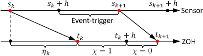
Figure 2: Switching between the subsystems of (21)

Though for both $\chi(t)=0$ and $\chi(t)=1$ the system (21) includes time-delays, the upper bound $\eta_{M}$ for $\bar{\eta}(t)$ is smaller than $\tau_{M}$ since $\tau(t)$ includes the delay due to sampling.

Define $\tau(t)=\bar{\eta}(t)$ for $t\in[\min\{t_{k}+h,t_{k+1}\},t_{k+1})$. We say that the system (10), (20) has an $L_{2}$-gain ($H_{\infty}$ gain) less than $\gamma$ if for the zero initial condition $x(0)=0$ and all $w,v\in L_{2}[0,\infty)$ such that $w^{T}(t)w(t)+v^{T}(t-\tau(t))v(t-\tau(t))\not\equiv 0$ the following relation holds on the trajectories of (10), (20):

$$J=\int_{0}^{\infty}\Bigl{\{}z^{T}(t)z(t)-\gamma^{2}[w^{T}(t)w(t)+v^{T}(t-\tau(t))v(t-\tau(t))]\Bigr{\}}\,dt<0.$$ (23)

Theorem 2.

For given $\gamma>0$, $h>0$, $\eta_{M}\geq 0$, $\varepsilon\geq 0$, $\delta>0$ let there exist $n\times n$ matrices $P>0$, $S_{0}\geq 0$, $S_{1}\geq 0$, $R_{0}\geq 0$, $R_{1}\geq 0$, $G_{1}$, $G_{0}$ and $l\times l$ matrix $\Omega\geq 0$ such that

$$\Psi\leq 0,\quad\Phi\leq 0,\quad\left[\begin{matrix}R_{0}&G_{0}\\ G_{0}^{T}&R_{0}\end{matrix}\right]\geq 0,\quad\left[\begin{matrix}R_{1}&G_{1}\\ G_{1}^{T}&R_{1}\end{matrix}\right]\geq 0,$$ (24)

where $\Psi=\{\Psi_{ij}\}$ and $\Phi=\{\Phi_{ij}\}$ are symmetric matrices composed from the matrices

$$\begin{array}[]{l}\Psi_{11}=\Phi_{11}=A^{T}P+PA+2\delta P+S_{0}-e^{-2\delta\eta_{M}}R_{0}+C_{1}^{T}C_{1},\\ \Psi_{12}=e^{-2\delta\eta_{M}}R_{0},\\ \Psi_{14}=PB_{2}KC_{2}+C_{1}^{T}D_{1}KC_{2},\\ \Psi_{15}=\Phi_{16}=PB_{1},\\ \Psi_{16}=\Phi_{17}=PB_{2}KD_{2}+C_{1}^{T}D_{1}KD_{2},\\ \Psi_{17}=\Phi_{18}=A^{T}H,\\ \Psi_{22}=\Phi_{22}=e^{-2\delta\eta_{M}}(S_{1}-S_{0}-R_{0})-e^{-2\delta\tau_{M}}R_{1},\\ \Psi_{23}=e^{-2\delta\tau_{M}}G_{1},\\ \Psi_{24}=e^{-2\delta\tau_{M}}(R_{1}-G_{1}),\\ \Psi_{33}=\Phi_{33}=-e^{-2\delta\tau_{M}}(R_{1}+S_{1}),\\ \Psi_{34}=e^{-2\delta\tau_{M}}(R_{1}-G_{1}^{T}),\\ \Psi_{44}=e^{-2\delta\tau_{M}}(G_{1}+G_{1}^{T}-2R_{1})+(D_{1}KC_{2})^{T}D_{1}KC_{2},\\ \Psi_{46}=(D_{1}KC_{2})^{T}D_{1}KD_{2},\\ \Psi_{47}=\Phi_{48}=(B_{2}KC_{2})^{T}H,\,\Psi_{55}=\Phi_{66}=-\gamma^{2}I,\\ \Psi_{57}=\Phi_{68}=B_{1}^{T}H,\\ \Psi_{77}=\Phi_{88}=-H,\\ \end{array}$$

$$\begin{array}[]{l}\Psi_{66}=(D_{1}KD_{2})^{T}D_{1}KD_{2}-\gamma^{2}I,\\ \Psi_{67}=\Phi_{78}=(B_{2}KD_{2})^{T}H,\\ \Phi_{12}=e^{-2\delta\eta_{M}}G_{0},\\ \Phi_{14}=PB_{2}KC_{2}+e^{-2\delta\eta_{M}}(R_{0}-G_{0})+C_{1}^{T}D_{1}KC_{2},\\ \Phi_{23}=e^{-2\delta\tau_{M}}R_{1},\\ \Phi_{24}=e^{-2\delta\eta_{M}}(R_{0}-G_{0}^{T}),\\ \Phi_{15}=PB_{2}K+C_{1}^{T}D_{1}K,\\ \Phi_{44}=e^{-2\delta\eta_{M}}(G_{0}+G_{0}^{T}-2R_{0})+(D_{1}KC_{2})^{T}D_{1}KC_{2}+\varepsilon C_{2}^{T}\Omega C_{2},\\ \Phi_{45}=(D_{1}KC_{2})^{T}D_{1}K,\\ \Phi_{47}=(D_{1}KC_{2})^{T}D_{1}KD_{2}+\varepsilon C_{2}^{T}\Omega D_{2},\\ \Phi_{55}=(D_{1}K)^{T}D_{1}K-\Omega,\\ \Phi_{57}=(D_{1}K)^{T}D_{1}KD_{2},\\ \Phi_{58}=(B_{2}K)^{T}H,\\ \Phi_{77}=(D_{1}KD_{2})^{T}D_{1}KD_{2}+\varepsilon D_{2}^{T}\Omega D_{2}-\gamma^{2}I,\\ H=\eta_{M}^{2}R_{0}+h^{2}R_{1},\end{array}$$

$\tau_{M}=h+\eta_{M}$, other blocks are zero matrices. Then the system (20) under the event-trigger (10) is internally exponentially stable with a decay rate $\delta$ and has $L_{2}$-gain less than $\gamma$.

Proof: See Appendix.

Corollary 1.

If (24) are valid with $C_{1}=0$, $D_{1}=0$ then the system (21) under the event-trigger (10) is Input-to-State Stable with respect to $\bar{w}(t)=\operatorname{col}\{w(t),v(t-\tau(t))\}$.

Proof. If $\bar{w}^{T}(t)\bar{w}(t)$ is bounded by $\Delta^{2}$ then (31) (see Appendix) with $C_{1}=0$, $D_{1}=0$ transforms to $\dot{V}\leq-2\delta V+\gamma^{2}\Delta^{2}$. This implies the assertion of the corollary.

$\square$

Remark 3.

The system (20) under periodic event-trigger (5) can be presented in the form (21) with $\chi=0$ and $\bar{\eta}(t)\leq\tau_{M}$. By modifying the proof of Theorem 2 one can obtain the stability conditions using the functional (26) with arbitrary chosen “delay partitioning” parameter $\eta_{M}\in(0,\tau_{M})$ [20, 21].

Remark 4.

The proposed approach can take into account packet dropouts with bounded amount of consecutive packet losses and acknowledgement signal of successful reception as suggested in, e.g., [22].

Remark 5.

Differently from periodic event-trigger approach considered in [9] our method is applicable to linear systems with polytopic-type uncertainties, since LMIs of Theorems 1 and 2 are affine in $A$, $B$, $B_{1}$, and $B_{2}$.

Remark 6.

MATLAB codes for solving the LMIs of Theorems 1, 2, Remarks 1, 3 are available at https://github.com/AntonSelivanov/TAC16.

4 Numerical examples

Example 1 [7]

Consider the system (3) with

$$A=\begin{bmatrix}0&1\\ -2&3\end{bmatrix},\quad B=\begin{bmatrix}0\\ 1\end{bmatrix},\quad C=I,\quad K=\begin{bmatrix}-1&4\end{bmatrix}.$$

For $\varepsilon=0$ (10) transforms into periodic sampling, therefore, Theorem 1 can be used to obtain the maximum period $h$. Under periodic sampling the amount of sent measurements is $\left[\frac{T_{f}}{h}\right]+1$, where $T_{f}$ is the time of simulation and $[\cdot]$ is the integer part of a given number. To obtain the amount of sent measurements for $t_{k}$ given by (5) (or (10)), for each $\varepsilon=i\times 10^{-4}$ ($i=0,\ldots,10^{4}$) we find the maximum $h$ that satisfies the conditions of Remark 1 (or Theorem 1) and for each pair of $(\varepsilon,h)$ we perform numerical simulations with $T_{f}=20$ for several initial conditions given by

$$(x_{1}(0),x_{2}(0))=\left(10\cos\left(\frac{2\pi}{30}\,k\right),10\sin\left(\frac{2\pi}{30}\,k\right)\right)$$

with $k=1,\ldots,30$. Then we choose the pair $(\varepsilon,h)$ that ensures the minimum average amount of sent measurements. In this example the best result was achieved under periodic sampling ($\varepsilon=0$). Theorem 1 gives $h=0.356$ for $\delta=0.24$ and $h=0.424$ for $\delta=0.001$. Both event-triggers (5) and (10) did not succeed in reducing the network workload.

Example 2 [8]

Consider the system (3) with

$$A=\left[\begin{matrix}0&1\\ 0&-3\end{matrix}\right],\quad B=\left[\begin{matrix}0\\ 1\end{matrix}\right],\quad C=\left[\begin{matrix}1&0\end{matrix}\right],\quad K=3.$$ (25)

Table 1: Example 2. Average amounts of sent measurements (SM)

	$\varepsilon$	$h$	SM
Periodic sampling	—	$1.173$	$18$
Event-trigger (5)	$4.6\times 10^{-3}$	$1.115$	$17.47$
Event-trigger (5)	$0.555$	$0.344$	$24.8$
Switching approach (10)	$0.555$	$0.899$	$11.13$

Table 2: Example 2. Average amounts of sent measurements (SM) for different $\eta_{M}$

	$\eta_{M}$	$0.1$	$0.2$	$0.4$	$0.6$	$0.7$
Period. samp./ event-tr. (5)	h	$0.636$	$0.548$	$0.355$	$0.143$	$0.025$
	SM	$33$	$38$	$57.33$	$139.27$	$785.73$
Event- trigger (10)	$\varepsilon$	$0.56$	$0.345$	$0.075$	$0.005$	$0$
	$h$	$0.339$	$0.379$	$0.278$	$0.12$	$0.025$
	SM	$23.7$	$28.5$	$52.4$	$137.77$	$785.73$

As it has been shown in [8] for this system an accumulation of events occurs under continuous event-trigger (4). In what follows we compare three approaches of choosing the sampling instants $s_{k}$: periodic sampling with $s_{k}=kh$, periodic event-trigger (5), and switching event-trigger (10).

We obtained the amount of sent measurements as described in Example 1 (taking $\delta=0.24$, $T_{f}=20$). As one can see from Table 1 periodic event-triggered (5) does not give any significant improvement compared to periodic sampling, while the event-trigger (10) allows to reduce the average amount of sent measurements by almost $40\%$. In Figs. 4  and 4 one can see the results of numerical simulations for the event-triggers (5) and (10). The vertical lines correspond to the time instants when the measurements are sent. The event-trigger (5) allows to skip the sending of two measurements (after $t_{4}$ and $t_{10}$), while (10) results in large inter sampling times $[t_{2},t_{3}]$, $[t_{4},t_{5}]$, etc. This allows to significantly reduce the network workload while the decay rate of convergence is preserved.

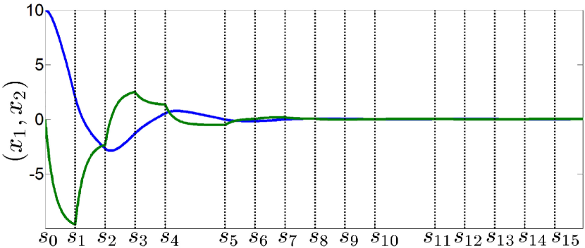
Figure 3: Example 2. Event-trigger (5): simulation of the system (3), (25), where $\varepsilon=4.6\times 10^{-3}$, $h=1.115$, $[x_{1}(0),x_{2}(0)]=[10,0]$ ($\eta_{M}=0$).

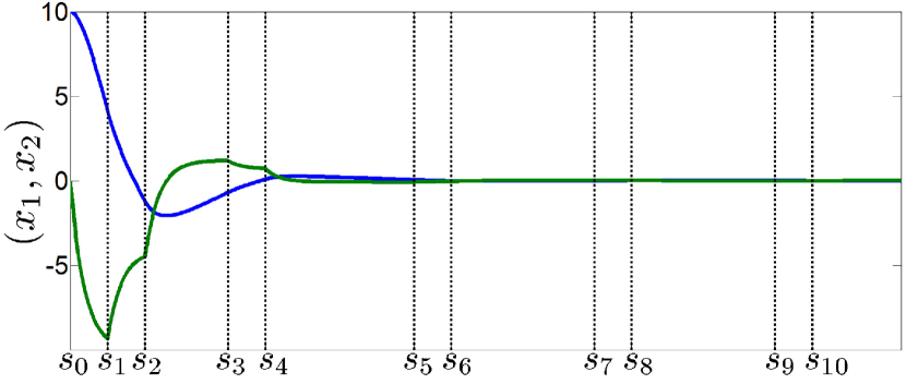
Figure 4: Example 2. Event-trigger (10): simulation of the system (3), (25), where $\varepsilon=0.555$, $h=0.899$, $[x_{1}(0),x_{2}(0)]=[10,0]$ ($\eta_{M}=0$).

Now we study the system (3) under network delays. According to the numerical simulations periodic event-trigger (5) does not give any improvement compared to the periodic sampling for any choice of $\eta_{M}$ (Remark 3). Using Theorem 2 with $B_{2}=B$, $C_{2}=C$ and other matrices equal to zero we obtained the values of $h$ and $\varepsilon$ in a manner similar to the previously described one. The delays $\eta_{k}\leq\eta_{M}$ have been chosen randomly subject to (19). The values of $\varepsilon$ and $h$ for $\delta=0.24$ and the corresponding average amounts of sent measurements (SM) during $20$ seconds of simulations for different maximum allowable delays $\eta_{M}$ are given in Table 2. As one can see the reduction in the amount of sent measurements vanishes when $\eta_{M}$ gets larger. This is due to the fact that with the increase of $\eta_{M}$ the sampling $h$ that preserves the stability is getting smaller, therefore, the difference between $\tau(t)$ and $\bar{\eta}(t)$ in (21) is getting less significant and the error separation principle proposed here loses its efficiency. However, for $\eta_{M}=0.1$ the switching approach (10) reduces the average amount of the sent measurements by almost $20\%$ while the decay rate of convergence $\delta$ is preserved.

Example 3 [16]

Table 3: Example 3. Amounts of sent measurements (SM) with time-delays and disturbances

	$\varepsilon$	$h$	SM
Periodic sampling	—	$0.091$	$330$
Event-trigger (5)	$0.033$	$0.036$	$195$
Event-trigger (10)	$0.044$	$0.065$	$173$

Consider an inverted pendulum on a cart described by (3) with

$$A=\left[\begin{matrix}0&1&0&0\\ 0&0&-1&0\\ 0&0&0&1\\ 0&0&10/3&0\end{matrix}\right],\quad B=\left[\begin{matrix}0\\ 0.1\\ 0\\ -1/30\end{matrix}\right],\quad C=I.$$

For $K=-[2,12,378,210]$ Theorem 1 gives $h=0.242$, $\varepsilon=0.35$. According to the numerical simulations, performed for $T_{f}$ and $x(0)$ from [16], the average release period under switching event-trigger (10) is $0.5769$, which is larger than $0.5131$ obtained for the same system in [11] (where the average release period is larger than in [23, 16, 24, 25]).

Consider the system (20) with the same $A$, $B_{1}^{T}=C_{1}=[1,1,1,1]$, $B_{2}=B$, $C_{2}=I$, $D_{1}=0.1$, $D_{2}=[0,0,0,0]^{T}$, $K=[2.9129,10.4357,287.9029,160.3271]$. For $\gamma=200$, $\eta_{M}=0.1$ Theorem 2 (with $\delta=0$) gives $h=0.117$, $\varepsilon=0.13$. From the numerical simulations, performed for $T_{f}$ and $w(t)$ from [11], we obtained an average release period $0.3488$, which is larger than $0.3098$ obtained for the same system in [11] (where the average release period is larger than the one obtained in [16] for a different controller gain).

For $\gamma=100$ in a manner similar to Example 1 we obtained the amount of sent measurements presented in Table 3. As one can see both event-triggers reduce the network workload and switching event-trigger (10) allows to reduce the amount of sent measurements by more than $11\%$ compared to periodic event-trigger (5).

5 Conclusion

We proposed a new approach to event-triggered control under the continuous-time measurements that guarantees a positive lower bound for inter-event times and can significantly reduce the workload of the network. Our idea is based on a switching between periodic sampling and continuous event-trigger. We extended this approach to the $L_{2}$-gain and ISS analyses of perturbed NCS with network-induced delays. Our results are applicable to linear systems with polytopic-type uncertainties. The presented method can be extended to nonlinear NCSs that may be a topic for the future research.

Appendix
Proof of Theorem 2

The system (10), (20) is rewritten as (21). Similar to [20] we consider Lyapunov functional

$$V=V_{P}+V_{S_{0}}+V_{S_{1}}+V_{R_{0}}+V_{R_{1}},$$ (26)

where $x_{t}(\theta)=x(t+\theta)$ for $\theta\in[-h,0]$, $V_{P}(x_{t})=x^{T}(t)Px(t)$,

$$V_{S_{0}}(t,x_{t}) =\int_{t-\eta_{M}}^{t}e^{2\delta(s-t)}x^{T}(s)S_{0}x(s)\,ds,$$

$$V_{R_{0}}(t,x_{t}) =\eta_{M}\int_{-\eta_{M}}^{0}\int_{t+\theta}^{t}e^{2\delta(s-t)}\dot{x}^{T}(s)R_{0}\dot{x}(s)\,ds\,d\theta,$$

$$V_{S_{1}}(t,x_{t}) =\int_{t-\tau_{M}}^{t-\eta_{M}}e^{2\delta(s-t)}x^{T}(s)S_{1}x(s)\,ds,$$

$$V_{R_{1}}(t,x_{t}) =h\int_{-\tau_{M}}^{-\eta_{M}}\int_{t+\theta}^{t}e^{2\delta(s-t)}\dot{x}^{T}(s)R_{1}\dot{x}(s)\,ds\,d\theta.$$

By differentiating these functionals we obtain

$$\dot{V}_{S_{0}} =-2\delta V_{S_{0}}+x^{T}(t)S_{0}x(t)-e^{-2\delta\eta_{M}}x^{T}(t-\eta_{M})S_{0}x(t-\eta_{M}),$$ (27)

$$\dot{V}_{S_{1}} =-2\delta V_{S_{1}}+e^{-2\delta\eta_{M}}x^{T}(t-\eta_{M})S_{1}x(t-\eta_{M})-e^{-2\delta\tau_{M}}x^{T}(t-\tau_{M})S_{1}x(t-\tau_{M}),$$

$$\dot{V}_{R_{0}} =-2\delta V_{R_{0}}+\eta_{M}^{2}\dot{x}^{T}(t)R_{0}\dot{x}(t)-\eta_{M}\int_{t-\eta_{M}}^{t}e^{2\delta(s-t)}\dot{x}^{T}(s)R_{0}\dot{x}(s)\,ds,$$

$$\dot{V}_{R_{1}} =-2\delta V_{R_{1}}+h^{2}\dot{x}^{T}(t)R_{1}\dot{x}(t)-h\int_{t-\tau_{M}}^{t-\eta_{M}}e^{2\delta(s-t)}\dot{x}^{T}(s)R_{1}\dot{x}(s)\,ds.$$

A. System (21) with $\chi(t)=0$, $\bar{\eta}(t)\in[0,\eta_{M}]$. We have

$$\dot{V}_{P}=2x^{T}(t)P[Ax(t)+B_{1}w(t)+B_{2}KC_{2}x(t-\bar{\eta}(t))+B_{2}KD_{2}v(t-\bar{\eta}(t))+B_{2}Ke(t)].$$ (28)

To compensate $x(t-\bar{\eta}(t))$ we apply Jensen’s inequality [26] and Park’s theorem [27] to obtain

$$-\eta_{M}\int_{t-\eta_{M}}^{t}e^{2\delta(s-t)}\dot{x}^{T}(s)R_{0}\dot{x}(s)\,ds\leq-e^{-2\delta\eta_{M}}\left[\begin{smallmatrix}x(t)-x(t-\bar{\eta}(t))\\ x(t-\bar{\eta}(t))-x(t-\eta_{M})\end{smallmatrix}\right]^{T}\left[\begin{smallmatrix}R_{0}&G_{0}\\ G_{0}^{T}&R_{0}\end{smallmatrix}\right]\left[\begin{smallmatrix}x(t)-x(t-\bar{\eta}(t))\\ x(t-\bar{\eta}(t))-x(t-\eta_{M})\end{smallmatrix}\right],$$ (29)

$$-h\int_{t-\tau_{M}}^{t-\eta_{M}}e^{2\delta(s-t)}\dot{x}^{T}(s)R_{1}\dot{x}(s)ds\leq-e^{-2\delta\tau_{M}}[x(t-\eta_{M})-x(t-\tau_{M})]^{T}R_{1}[x(t-\eta_{M})-x(t-\tau_{M})].$$ (30)

By summing up (22), (27), (28) in view of (29) and (30) and substituting $z$ from (21) we obtain

$$\dot{V}+2\delta V+z^{T}z-\gamma^{2}[w^{T}w+v^{T}(t-\bar{\eta}(t))v(t-\bar{\eta}(t))]\leq\varphi^{T}(t)\Phi^{\prime}\varphi(t)+\dot{x}^{T}(t)H\dot{x}(t),$$

where $\varphi(t)=\operatorname{col}\{x(t),x(t-\eta_{M}),x(t-\tau_{M}),x(t-\bar{\eta}(t)),e(t),w(t),v(t-\bar{\eta}(t))\}$ and the matrix $\Phi^{\prime}$ is obtained from $\Phi$ by deleting the last block-column and the last block-row. Substituting expression for $\dot{x}$ and applying Schur complement formula we find that $\Phi\leq 0$ guarantees that

$$\dot{V}+2\delta V+z^{T}z-\gamma^{2}[w^{T}w+v^{T}(t-\tau(t))v(t-\tau(t))]\leq 0.$$ (31)

B. System (21) with $\chi=1$, $\tau(t)\in(\eta_{M},\tau_{M}]$. For $\tau(t)\in[0,\eta_{M}]$ the system (21) with $\chi=1$ is described by (21) with $\chi=0$ and $e(t)=0$ satisfying (22). That is, $\Phi\leq 0$ guarantees (31) for (21) with $\chi=1$, $\tau(t)\in[0,\eta_{M}]$. Therefore, we study the system (21) for $\chi=1$, $\tau(t)\in(\eta_{M},\tau_{M}]$. We have

$$\dot{V}_{P}=2x^{T}(t)P[Ax(t)+B_{1}w(t)+B_{2}KC_{2}x(t-\tau(t))+B_{2}KD_{2}v(t-\tau(t))].$$ (32)

To compensate $x(t-\tau(t))$ with $\tau(t)\in(\eta_{M},\tau_{M}]$ we apply Jensen’s inequality and Park’s theorem to obtain

$$-\eta_{M}\int_{t-\eta_{M}}^{t}e^{2\delta(s-t)}\dot{x}^{T}(s)R_{0}\dot{x}(s)\,ds\leq-e^{-2\delta\eta_{M}}[x(t)-x(t-\eta_{M})]^{T}R_{0}[x(t)-x(t-\eta_{M})],$$ (33)

$$-h\int_{t-\tau_{M}}^{t-\eta_{M}}e^{2\delta(s-t)}\dot{x}^{T}(s)R_{1}\dot{x}(s)ds\leq-e^{-2\delta\tau_{M}}\left[\begin{smallmatrix}x(t-\eta_{M})-x(t-\tau(t))\\ x(t-\tau(t))-x(t-\tau_{M})\end{smallmatrix}\right]^{T}\left[\begin{smallmatrix}R_{1}&G_{1}\\ G_{1}^{T}&R_{1}\end{smallmatrix}\right]\left[\begin{smallmatrix}x(t-\eta_{M})-x(t-\tau(t))\\ x(t-\tau(t))-x(t-\tau_{M})\end{smallmatrix}\right].$$ (34)

By summing up (27) and (32) in view of (33) and (34) and substituting $z$ from (21) we obtain

$$\dot{V}+2\delta V+z^{T}z-\gamma^{2}[w^{T}w+v^{T}(t-\tau(t))v(t-\tau(t))]\leq\psi^{T}(t)\Psi^{\prime}\psi(t)+\dot{x}^{T}(t)H\dot{x}(t),$$

where $\psi(t)=\operatorname{col}\{x(t),x(t-\eta_{M}),x(t-\tau_{M}),x(t-\tau(t)),w(t),v(t-\tau(t))\}$ and the matrix $\Psi^{\prime}$ is obtained from $\Psi$ by deleting the last block-column and the last block-row. Substituting expression for $\dot{x}$ and applying Schur complement formula we find that $\Psi\leq 0$ guarantees (31) for (21) with $\chi=1$.

Thus, (31) is true for the switched system (21). For $w\equiv 0$, $v\equiv 0$ (31) implies $\dot{V}\leq-2\delta V$. Therefore, the system (21) is internally exponentially stable with the decay rate $\delta$. By integrating (31) from $0$ to $\infty$ with $x(0)=0$ we obtain (23).

References

- [1] A. Selivanov and E. Fridman, “A Switching Approach to Event-Triggered Control,” in 54st IEEE Conference on Decision and Control, 2015.
- [2] ——, “Event-Triggered Control: A Switching Approach,” IEEE Transactions on Automatic Control, vol. 61, no. 10, pp. 3221–3226, 2016.
- [3] P. J. Antsaklis and J. Baillieul, “Guest Editorial Special Issue on Networked Control Systems,” IEEE Transactions on Automatic Control, vol. 49, no. 9, pp. 1421–1423, 2004.
- [4] J. Hespanha, P. Naghshtabrizi, and Y. Xu, “A Survey of Recent Results in Networked Control Systems,” Proceedings of the IEEE, vol. 95, no. 1, 2007.
- [5] E. Garcia and P. J. Antsaklis, “Model-based event-triggered control for systems with quantization and time-varying network delays,” IEEE Transactions on Automatic Control, vol. 58, no. 2, pp. 422–434, 2013.
- [6] E. Fridman, Introduction to Time-Delay Systems: Analysis and Control. Birkhäuser Basel, 2014.
- [7] P. Tabuada, “Event-Triggered Real-Time Scheduling of Stabilizing Control Tasks,” IEEE Transactions on Automatic Control, vol. 52, no. 9, pp. 1680–1685, 2007.
- [8] D. Borgers and W. P. M. H. Heemels, “Event-separation properties of event-triggered control systems,” IEEE Transactions on Automatic Control, vol. 59, no. 10, pp. 2644–2656, 2014.
- [9] W. P. M. H. Heemels, M. C. F. Donkers, and A. R. Teel, “Periodic Event-Triggered Control for Linear Systems,” IEEE Transactions on Automatic Control, vol. 58, no. 4, pp. 847–861, 2013.
- [10] C. Peng and T. C. Yang, “Event-triggered communication and control co-design for networked control systems,” Automatica, vol. 49, no. 5, pp. 1326–1332, 2013.
- [11] D. Yue, E. Tian, and Q.-L. Han, “A delay system method for designing event-triggered controllers of networked control systems,” IEEE Transactions on Automatic Control, vol. 58, no. 2, pp. 475–481, 2013.
- [12] X.-M. Zhang and Q.-L. Han, “Event-triggered dynamic output feedback control for networked control systems,” IET Control Theory & Applications, vol. 8, no. 4, pp. 226–234, 2014.
- [13] W. P. M. H. Heemels, J. H. Sandee, and P. P. J. Van Den Bosch, “Analysis of event-driven controllers for linear systems,” International Journal of Control, vol. 81, no. 4, pp. 571–590, 2008.
- [14] P. Tallapragada and N. Chopra, “Event-triggered dynamic output feedback control for LTI systems,” in 51st IEEE Conference on Decision and Control, 2012, pp. 6597–6602.
- [15] ——, “Event-Triggered Decentralized Dynamic Output Feedback Control for LTI Systems,” in IFAC Workshop on Distributed Estimation and Control in Networked Systems, 2012, pp. 31–36.
- [16] X. Wang and M. D. Lemmon, “Self-Triggered Feedback Control Systems With Finite-Gain Stability,” IEEE Transactions on Automatic Control, vol. 54, no. 3, pp. 452–467, 2009.
- [17] A. L. Fradkov, “Passification of Non-square Linear Systems and Feedback Yakubovich-Kalman-Popov Lemma,” European Journal of Control, no. 6, pp. 573–582, 2003.
- [18] E. Fridman, A. Seuret, and J.-P. Richard, “Robust sampled-data stabilization of linear systems: an input delay approach,” Automatica, vol. 40, no. 8, pp. 1441–1446, 2004.
- [19] E. Fridman, “A refined input delay approach to sampled-data control,” Automatica, vol. 46, no. 2, pp. 421–427, 2010.
- [20] E. Fridman, U. Shaked, and K. Liu, “New conditions for delay-derivative-dependent stability,” Automatica, vol. 45, no. 11, pp. 2723–2727, 2009.
- [21] Y. Guan, “Analysis and Design of Event-Triggered Networked Control Systems,” Ph.D. dissertation, Central Queensland University, 2013.
- [22] M. Guinaldo, D. Lehmann, J. Sánchez, S. Dormido, and K. H. Johansson, “Distributed event-triggered control with network delays and packet losses,” in 51st IEEE Conference on Decision and Control, 2012, pp. 1–6.
- [23] X. Wang, “Event-Triggering in Cyber-Physical Systems,” Ph.D. dissertation, The University of Notre Dame, 2009.
- [24] D. Carnevale, A. R. Teel, and D. Nešić, “Further results on stability of networked control systems: A Lyapunov approach,” in American Control Conference, 2007, pp. 1741–1746.
- [25] P. Tabuada and X. W. X. Wang, “Preliminary results on state-trigered scheduling of stabilizing control tasks,” 45th IEEE Conference on Decision and Control, pp. 282–287, 2006.
- [26] K. Gu, V. L. Kharitonov, and J. Chen, Stability of Time-Delay Systems. Boston: Birkhäuser, 2003.
- [27] P. Park, J. W. Ko, and C. Jeong, “Reciprocally convex approach to stability of systems with time-varying delays,” Automatica, vol. 47, no. 1, pp. 235–238, 2011.