Coherent network analysis for continuous gravitational wave signals in a pulsar timing array: Pulsar phases as extrinsic parameters

Abstract

Supermassive black hole binaries are one of the primary targets for gravitational wave searches using pulsar timing arrays. Gravitational wave signals from such systems are well represented by parametrized models, allowing the standard Generalized Likelihood Ratio Test (GLRT) to be used for their detection and estimation. However, there is a dichotomy in how the GLRT can be implemented for pulsar timing arrays: there are two possible ways in which one can split the set of signal parameters for semi-analytical and numerical extremization. The straightforward extension of the method used for continuous signals in ground-based gravitational wave searches, where the so-called pulsar phase parameters are maximized numerically, was addressed in an earlier paper (Wang et al., 2014). In this paper, we report the first study of the performance of the second approach where the pulsar phases are maximized semi-analytically. This approach is scalable since the number of parameters left over for numerical optimization does not depend on the size of the pulsar timing array. Our results show that, for the same array size (9 pulsars), the new method performs somewhat worse in parameter estimation, but not in detection, than the previous method where the pulsar phases were maximized numerically. The origin of the performance discrepancy is likely to be in the ill-posedness that is intrinsic to any network analysis method. However, scalability of the new method allows the ill-posedness to be mitigated by simply adding more pulsars to the array. This is shown explicitly by taking a larger array of pulsars.

1 Introduction

Pulsar timing array (PTA) based gravitational wave (GW) search is a promising approach for the very low frequency ($\sim 10^{-9}-10^{-6}$ Hz) regime (Sazhin, 1978; Foster & Backer, 1990; Jenet et al., 2005), that is complimentary to the second-generation ground-based interferometers, such as Advanced LIGO (Waldman, 2011), Advanced Virgo (Degallaix et al., 2013), and KAGRA (Somiya, 2012) operating at high frequencies ($\sim 10-10^{3}$ Hz), as well as to the space-based detectors, such as eLISA (Seoane et al., 2013) proposed for low frequencies ($\sim 10^{-4}-10^{-1}$ Hz). Unlike man-made instruments, PTA uses a network of high precision astronomical clocks, i.e., millisecond pulsars (MSPs), as a galactic-scale GW detector. Currently, three regional PTAs (NANOGrav, PPTA and EPTA) are operating at astrophysically interesting sensitivities that may lead to the detection of GWs in the near future. Shared data as well as collaborative and competitive efforts among individual PTAs bond them as the International Pulsar Timing Array (IPTA, Manchester (2013); McLaughlin (2014)). The IPTA uses some of the most advanced radio telescopes in the world today to regularly monitor about 50 pulsars. Next generation radio telescopes with larger collecting areas and better backend systems, such as FAST (Hobbs et al., 2014) and SKA (Smits et al., 2009), will join the global observation campaign in the future and push pulsar timing to higher precision and better detection sensitivities.

A promising GW signal for PTA is the stochastic background formed by the incoherent superposition of weak signals from a large unresolved population of supermassive black hole binaries (SMBHBs) (Detweiler, 1979; Romani & Taylor, 1983; Foster & Backer, 1990; Jaffe & Backer, 2003; Wyithe & Loeb, 2003; Jenet et al., 2005). The stochastic GW perturbation will cause noise like signals in the pulsar time of arrivals (TOAs) that will be correlated across the pulsars in an array. The correlation will depend on the strength of the stochastic background and the pair-wise angular separation between the pulsars (Hellings & Downs, 1983). Upper limits on the strength of the stochastic background along with our understanding of source population have been improving over the years in correspondence with improvements in data quality (Jenet et al., 2006; Yardley et al., 2011; van Haasteren et al., 2011; Shannon et al., 2013; Demorest et al., 2013).

In addition to the stochastic background, there exists the interesting possibility of detecting GWs from individual SMBHB sources (Detweiler, 1979; Lommen & Backer, 2001; Jenet et al., 2004; Seto, 2009). Simulations covering a range of massive black hole population models (Sesana et al., 2009; Sesana & Vecchio, 2010) have shown that on average at least one source may be resolvable against the stochastic background. In the past few years, interest in analyzing continuous GW signals from individual SMBHBs has increased considerably (Lee et al., 2011; Deng & Finn, 2011; Mingarelli et al., 2012; Ravi et al., 2014). Correspondingly, searches for continuous signals in the recent PTA data have been conducted in parallel with the stochastic background (Yardley et al., 2010; Arzoumanian et al., 2014; Zhu et al., 2014).

The detection and parameter estimation of continuous waves from individual sources in a PTA is a challenging data analysis task that has led to a number of studies (Yardley et al., 2010; Corbin & Cornish, 2010; Babak & Sesana, 2012; Ellis et al., 2012; Ellis, 2013; Wang et al., 2014; Taylor et al., 2014; Zhu et al., 2015). Unlike ground and space based detectors, the analysis of PTA data must contend with irregularly sampled time series with possible gaps, and noise components that must be estimated along with the signal as well as components that may be non-Gaussian or non-stationary (Wang & et al., 2015). As with any complex data analysis problem, a wide range of independent and complementary approaches are needed to build confidence in the final results.

This paper follows an earlier investigation reported in Wang et al. (2014) (hereafter WMJ1), where a Generalized Likelihood Ratio Test (GLRT) (Kay, 1998) was constructed along the line of existing continuous wave signal searches used for ground based detectors (Jaranowski et al., 1998; Cutler & Schutz, 2005). The WMJ1 method explicitly includes the pulsar terms in the signal model and considers them as functions of pulsar phases. Numerical implementation of the GLRT usually involves a division of the signal parameters into the so-called extrinsic ones, over which the likelihood ratio can be maximized analytically or semi-analytically (including the use of Fast Fourier Transform), and the intrinsic ones for which a pure numerical optimization is required. However, unlike the ground based search, this division of the parameters into extrinsic and intrinsic is not unique in the case of a PTA. Following the convention used for the $\mathcal{F}$-statistic (Jaranowski & Królak, 2012), WMJ1 explored the choice that takes the overall amplitude of the signal, the inclination angle between the binary orbit and the plane of the sky, and the polarization angle of the GW as extrinsic and treated the pulsar phases and remaining parameters as intrinsic. Our results showed that the pulsar phases are uninformative parameters, indicating that they are best marginalized or maximized as extrinsic parameters. The more important motivation to do so, however, is the fact that the number of pulsar phase parameters increases with the size of the PTA. Hence, the numerical optimization task will become infeasible at some point. Thus, the approach of treating pulsar phase parameters as intrinsic is not a scalable one.

This paper presents the first implementation of a method based on treating the pulsar phases as extrinsic parameters in a GLRT. Although, the idea of semi-analytical maximization over pulsar phases was presented in Ellis et al. (2012), a concrete implementation and performance characterization of the resulting method has not been reported until now. The method proposed here retains the use of Particle Swarm Optimization (PSO) to handle the numerical optimization over intrinsic parameters, but the particular variant of the PSO meta-heuristic used in this paper is different.

An alternative to maximization over the pulsar phases is to marginalize over them following a Bayesian framework. This is the approach that has been studied the most in the PTA literature so far (Ellis, 2013; Taylor et al., 2014). To enable meaningful comparisons, the performance of the method presented here is studied on simulated data corresponding to a PTA configuration adopted in Taylor et al. (2014). We use signal strengths, measured in terms of the network signal-to-noise ratio (S/N) $\rho_{n}$, that span a wide range from strong ($\rho_{n}=100$) to moderate ($\rho_{n}=30$) and barely detectable ($\rho_{n}=8$). Although useful for testing the performance of the algorithm, $\rho_{n}>20$ is unrealistic for PTA based GW detection in the foreseeable future. Thus the performance of the method for $\rho_{n}=8$ to $\rho_{n}=30$ serves to bracket the scenario that is more likely. As in WMJ1, we simulate a large number of independent data realizations and derive conventional Frequentist error estimates for the signal parameters.

The results show that this method performs marginally better than the method in WMJ1 for detection, but the estimation of the angular parameters is somewhat worse. Specifically, while the localization of sources in WMJ1 and the Bayesian method are comparable, shifting to a different split of extrinsic and intrinsic parameters creates secondary maxima that increase the scatter of estimated source locations. This is most likely the result of the well known ill-posedness of the GW network analysis problem (Klimenko et al., 2005; Rakhmanov, 2006; Mohanty et al., 2006). Ill-posedness in inverse problems, such as GW network analysis, is marked by instability or discontinuity of the inferred solution under small perturbations in the data. The source of perturbation can be either the noise in the data or numerical errors from computations. The jumping of solutions to radically different values can manifest itself as a large bias or large variance in estimation. For strictly linear models, such as GW burst searches where the time samples of the two polarization waveforms directly form the parameters to be estimated (Rakhmanov, 2006), ill-posedness is easily seen to be rooted in the rank deficiency of the matrix $A^{T}A$, where $A$ is the $m\times 2$ network response matrix ($m$ is the number of detectors). The origin of ill-posedness in parameter estimation presented in this work is not as straightforward because the signal model is nonlinear in the parameters.

Mitigation of ill-posedness requires regularization in some form, such as the imposition of constraints on the GLRT solutions (Greville, 1959; Tikhonov & Arsenin, 1977). While some constraints appear naturally in the implementation of GLRT in WMJ1, they are absent in the formulation of the method presented here. The effects of ill-posedness are reduced, in general, by increasing the number of differently oriented detectors in a network. We demonstrate this by considering the case of a PTA with 17 pulsars. For this reason, we do not go deeper into the issue of regularization for PTA in this paper but leave it for future work to address.

The rest of the paper is organized as follows. In Section 2 we introduce the data model used in this paper. Section 3 describes the GLRT for this data model and its implementation, which involves maximization over pulsar phases analytically by solving quartic equations. Section 4 characterizes the method using simulated data and compares its performance with WMJ1 and Taylor et al. (2014). The paper is concluded in Section 5. Some details about solving the quartic equation have been relegated to Appendix A.

2 Data model

The data used for GW signal detection and parameter estimation in the case of a PTA consists of a set of timing residuals $r^{I}=(r^{I}_{1},r^{I}_{2},\ldots,r^{I}_{N_{I}})$, $I=1,2,\ldots,N_{p}$, where $N_{p}$ is the number of pulsars, $N_{I}$ is the number of observation for the $I$-th pulsar. Each timing residual is associated with a time of observation $t^{I}_{i}\in[0,T]$, $t^{I}_{i+1}>t^{I}_{i}$. The time interval between two observations can vary typically from several days up to a few weeks. When there is a signal in the data, $r^{I}_{k}=s^{I}_{k}+n^{I}_{k}$; otherwise, $r^{I}_{k}=n^{I}_{k}$. Here $n^{I}=(n^{I}_{1},n^{I}_{2},\ldots,n^{I}_{n_{I}})$ and $s^{I}=(s^{I}_{1},s^{I}_{2},\ldots,s^{I}_{n_{I}})$ denote the noise realization and the GW signal respectively. The models for the signal and the noise (zero mean stationary Gaussian) remain the same as in WMJ1, but it is convenient to express the signal in a functional form that allows the pulsar phases to be easily extracted as extrinsic parameters in the detection statistic.

GWs perturb the proper distance between a pulsar and an observer on the Earth, causing fluctuations of the TOAs of radio pulses with time. In the TT-gauge associated with a plane GW, the perturbation in the metric tensor can be written as

$$\mathbf{h}=(h_{+}\mathbf{e}_{+}+h_{\times}\mathbf{e}_{\times})e^{i(\omega_{\text{gw}}t-\mathbf{k}\cdot\mathbf{x})}\,,$$ (1)

where $\omega_{\text{gw}}$ is the GW angular frequency, $\mathbf{k}$ is the GW wave vector, and

$$\mathbf{e}_{+}=\bm{\hat{\alpha}}\otimes\bm{\hat{\alpha}}-\bm{\hat{\delta}}\otimes\bm{\hat{\delta}}\,,$$ (2a)

$$\mathbf{e}_{\times}=\bm{\hat{\alpha}}\otimes\bm{\hat{\delta}}+\bm{\hat{\delta}}\otimes\bm{\hat{\alpha}}\,.$$ (2b)

$\bm{\hat{\alpha}}$ and $\bm{\hat{\delta}}$ are the unit vectors along right ascension and declination in equatorial coordinates. The response of the detector to the GW is given by

$$s^{I}_{i}(\lambda)=F^{I}_{+}(\alpha,\delta)\Delta h_{+}(t^{I}_{i};\theta)+F^{I}_{\times}(\alpha,\delta)\Delta h_{\times}(t^{I}_{i};\theta)\,,$$ (3)

where $F^{I}_{+}$ and $F^{I}_{\times}$ are the antenna pattern functions (defined in Equations 9 and 10 of WMJ1), $\alpha$ and $\delta$ are the right ascension and declination of the source, $\theta$ represents collectively the following parameters: (i) $\zeta$, the overall amplitude factor (defined in Equation 7 of WMJ1); (ii) $\iota$, the inclination angle between the binary orbital plane and the plane of the sky; (iii) $\psi$, the GW polarization angle; (iv) $\varphi_{0}$, the initial phase of the binary at the beginning of the observation; (v) parameter $\varphi_{I}=\varphi_{0}-\frac{1}{2}\omega_{\text{gw}}d^{I}(1-\cos\theta^{I})$, the pulsar phase parameter that contains the distance $d^{I}$ from the pulsar to Earth and the open angle $\theta^{I}$ between the lines of sight to the pulsar and the GW source. Hereafter, we regard the pulsar phases as independent variables. $\lambda=\{\alpha,\delta\}\cup\theta$ denotes the set of all the parameters. The term $\Delta h_{+,\times}(t^{I}_{i};\theta)$ is the difference of the GW tensor at Earth and at the pulsar at the observer’s time $t^{I}_{i}$,

$$\Delta h_{+,\times}(t^{I}_{i};\theta)=h_{+,\times}(t^{I}_{i};\theta)-h_{+,\times}(t^{I}_{i}-\tau^{I};\theta)\,,$$ (4)

where $\tau^{I}=d^{I}(1-\cos\theta^{I})/c$ is the time delay of the plane GWs of the same phase arriving at Earth and at the pulsar. Hereafter, we assume that the binary system is evolving slowly, so that in the signal model the orbital frequency in the pulsar term remains approximately the same as in the Earth term.

The GW signal can be written as

$$s^{I}_{i} = 2\zeta(1+\cos^{2}\iota)(F_{+}^{I}\cos 2\psi-F_{\times}^{I}\sin 2\psi)\sin(\varphi_{0}-\varphi_{I})\sin(\varphi_{0}+\varphi_{I}+\Phi(t^{I}_{i}))$$ (5)

$$- 4\zeta\cos\iota(F_{+}^{I}\sin 2\psi+F_{\times}^{I}\cos 2\psi)\sin(\varphi_{0}-\varphi_{I})\cos(\varphi_{0}+\varphi_{I}+\Phi(t^{I}_{i}))$$

$$= \mathcal{A}_{I}\sin(\varphi_{0}-\varphi_{I})\sin(\varphi_{0}+\varphi_{I}+\phi_{I}+\Phi(t^{I}_{i}))\,,$$

where $\Phi(t^{I}_{i})=\omega_{\rm gw}t_{i}^{I}$,

$$\mathcal{A}_{I}^{2} = 4\zeta^{2}(1+\cos^{2}\iota)^{2}(F_{+}^{I}\cos 2\psi-F_{\times}^{I}\sin 2\psi)^{2}$$ (6)

$$+ 16\zeta^{2}\cos^{2}\iota(F_{+}^{I}\sin 2\psi+F_{\times}^{I}\cos 2\psi)^{2}\,,$$

and

$$\tan\phi_{I}=\frac{-2\cos\iota}{1+\cos^{2}\iota}\cdot\frac{F_{+}^{I}\sin 2\psi+F_{\times}^{I}\cos 2\psi}{F_{+}^{I}\cos 2\psi-F_{\times}^{I}\sin 2\psi}\,.$$ (7)

Here $\mathcal{A}_{I}$ and $\phi_{I}$ depend only on $\zeta,\iota,\psi,\alpha,\delta$. In Equation 5, we can isolate the $\varphi_{I}$ dependence and get

$$s^{I}_{i}=(\mathcal{B}_{I}-\mathcal{E}_{I})\cos 2\varphi_{I}+(\mathcal{C}_{I}+\mathcal{D}_{I})\sin 2\varphi_{I}+(\mathcal{B}_{I}+\mathcal{E}_{I})\,,$$ (8)

where

$$\mathcal{B}_{I}(t^{I}_{i})=\frac{1}{2}\mathcal{A}_{I}\sin\varphi_{0}\sin(\varphi_{0}+\phi_{I}+\Phi(t^{I}_{i}))\,,$$ (9)

$$\mathcal{C}_{I}(t^{I}_{i})=-\frac{1}{2}\mathcal{A}_{I}\cos\varphi_{0}\sin(\varphi_{0}+\phi_{I}+\Phi(t^{I}_{i}))\,,$$ (10)

$$\mathcal{D}_{I}(t^{I}_{i})=\frac{1}{2}\mathcal{A}_{I}\sin\varphi_{0}\cos(\varphi_{0}+\phi_{I}+\Phi(t^{I}_{i}))\,,$$ (11)

$$\mathcal{E}_{I}(t^{I}_{i})=-\frac{1}{2}\mathcal{A}_{I}\cos\varphi_{0}\cos(\varphi_{0}+\phi_{I}+\Phi(t^{I}_{i}))\,.$$ (12)

Note that $\mathcal{B}_{I}$, $\mathcal{C}_{I}$, $\mathcal{D}_{I}$, $\mathcal{E}_{I}$ are functions of time and the source parameters rather than $\varphi_{I}$.

3 Generalized Likelihood Ratio Test

In the Frequentist approach, the detection of GW signals presents a composite hypotheses test problem: Given data ${\bf r}$, we need to pick one among a family of hypotheses about the joint probability density function (pdf) from which ${\bf r}$ is obtained. Under the null hypothesis $\mathcal{H}_{0}$, the data does not contain any GW signal and the pdf, $p({\bf r})$, governing ${\bf r}$ is that of the noise alone. Under the alternative hypothesis $H_{\lambda}$, a GW signal ${\bf s}(\lambda)$ with parameters $\lambda$ is present in ${\bf r}$ and the data is a realization from a governing pdf of the form $p({\bf r}|\lambda)=p({\bf r}-{\bf s}(\lambda))$. In a GLRT, assuming that the PDF of the noise $p(\mathbf{r})$ is known, the test statistic

$$\text{GLRT}(\mathbf{r})=\max_{\lambda}\frac{p(\mathbf{r}|\lambda)}{p(\mathbf{r})}=\max_{\lambda}\text{LR}(\mathbf{r};\lambda)=\text{LR}(\mathbf{r};\widehat{\lambda})\,,$$ (13)

is compared with a threshold to decide in favor of $\mathcal{H}_{0}$ or $\mathcal{H}_{\widehat{\lambda}}$. Here, $\text{LR}(\mathbf{r};\lambda)$ is the likelihood ratio for a given hypothesis and $\widehat{\lambda}$ is the Maximum Likelihood Estimate (MLE) of the parameters. The maximizer, $\widehat{\lambda}$, of $\text{LR}(\mathbf{r};\lambda)$ in Eq. 13 is the same as that of any monotonic function of $\text{LR}(\mathbf{r};\lambda)$. Its logarithm, $\Lambda(\mathbf{r};\lambda)$, is one such convenient choice for the case of Gaussian noise.

Unlike the case of a known $\lambda$, where the optimal test statistic (under the Neyman-Pearson criterion) is known to be $\text{LR}({\bf r};\lambda)$, there is no proof of optimality associated with the GLRT except in some simple cases. However, it has been shown that it is the uniformly most powerful (UMP) among all invariant tests (Lehmann, 1959). In practice, and when it is computationally feasible, the GLRT is often found to be superior to other ad hoc tests.

3.1 The network likelihood ratio

For a PTA of $N_{p}$ pulsars, the log-likelihood ratio is

$$\Lambda(\mathbf{r};\lambda) = \sum_{I=1}^{N_{p}}\Lambda_{I}({\bf r};\lambda)\;,$$

$$\Lambda_{I}({\bf r};\lambda) = \langle r^{I}|s^{I}(\lambda)\rangle_{I}-\frac{1}{2}\langle s^{I}(\lambda)|s^{I}(\lambda)\rangle_{I}\,,$$ (14)

where $\langle\cdot|\cdot\rangle_{I}$ is the noise weighted inner product, $(\cdot){\bf C}_{I}^{-1}(\cdot)^{T}$, with ${\bf C}_{I}$ being the covariance matrix of the noise process in the $I$-th pulsar. It is assumed here that the cross-covariances of noise between $r^{I}$ and $r^{J}$ are ignorable for $I\neq J$. Inserting Eq. 8 into Eq. 14 we have

$$\Lambda_{I}(\mathbf{r};\lambda) =\left[\langle r^{I}|X_{I}\rangle_{I}\cos 2\varphi_{I}+\langle r^{I}|Y_{I}\rangle_{I}\sin 2\varphi_{I}+\langle r^{I}|Z_{I}\rangle_{I}\right.$$

$$\left.-\frac{1}{2}\left(\langle X_{I}|X_{I}\rangle_{I}\cos^{2}2\varphi_{I}+\langle Y_{I}|Y_{I}\rangle_{I}\sin^{2}2\varphi_{I}+2\langle X_{I}|Y_{I}\rangle_{I}\sin 2\varphi_{I}\cos 2\varphi_{I}\right.\right.$$

$$+2\langle X_{I}|Z_{I}\rangle_{I}\cos 2\varphi_{I}+2\langle Y_{I}|Z_{I}\rangle_{I}\sin 2\varphi_{I}+\langle Z_{I}|Z_{I}\rangle_{I}\left.\left.\right)\right]\,,$$ (15)

where $X_{I}=\mathcal{B}_{I}-\mathcal{E}_{I}$, $Y_{I}=\mathcal{C}_{I}+\mathcal{D}_{I}$, and $Z_{I}=\mathcal{B}_{I}+\mathcal{E}_{I}$.

The calculation of the GLRT can be seen as a nested maximization problem,

$$\text{GLRT}(\mathbf{r})=\max_{\lambda_{i}}\max_{\lambda_{e}}\Lambda(\mathbf{r};\lambda)\,.$$ (16)

This split is meant to indicate that the whole model parameter set $\lambda$ can be divided into disjoint subsets classified as extrinsic (inner maximization) $\lambda_{e}=\{\varphi_{I}\}$, and intrinsic (outer maximization) $\lambda_{i}=\{\alpha,\delta,\omega_{\text{gw}},\zeta,\iota,\psi,\varphi_{0}\}$. Usually, the separation is made such that the former can be maximized using analytical (or semi-analytical) methods, while the latter requires computationally expensive numerical optimization. It should be emphasized that the classification of parameters as extrinsic (computationally trivial) and intrinsic (computationally non-trivial) pertains to their role in the numerical procedure adopted for their estimation rather than their role in defining the the astrophysical signal.

3.2 Maximization over extrinsic parameters

The inner maximization of the GLRT over the extrinsic parameters (Eq. 16) leads to,

$$c^{I}_{1}\sin 2\varphi_{I}+c^{I}_{2}\cos 2\varphi_{I}+c^{I}_{3}\sin 4\varphi_{I}+c^{I}_{4}\cos 4\varphi_{I}=0\,,$$ (17)

where

$$c^{I}_{1} =-\langle r^{I}|X_{I}\rangle_{I}+\langle X_{I}|Z_{I}\rangle_{I}\,,$$ (18a)

$$c^{I}_{2} =\langle r^{I}|Y_{I}\rangle_{I}-\langle Y_{I}|Z_{I}\rangle_{I}\,,$$ (18b)

$$c^{I}_{3} =\frac{1}{2}\big{(}\langle X_{I}|X_{I}\rangle_{I}-\langle Y_{I}|Y_{I}\rangle_{I}\big{)}\,,$$ (18c)

$$c^{I}_{4} =-\langle X_{I}|Y_{I}\rangle_{I}\,.$$ (18d)

By defining $y=\cos 2\varphi_{I}$, Eq. 17 can be transformed into a set of $N_{p}$ quartic equations

$$ay^{4}+by^{3}+cy^{2}+dy+e=0$$ (19)

where

$$a =4(c_{3}^{2}+c_{4}^{2})\,,$$ (20a)

$$b =4(c_{1}c_{3}+c_{2}c_{4})\,,$$ (20b)

$$c =c_{1}^{2}+c_{2}^{2}-4(c_{3}^{2}+c_{4}^{2})\,,$$ (20c)

$$d =-4c_{1}c_{3}-2c_{2}c_{4}\,,$$ (20d)

$$e =c_{4}^{2}-c_{1}^{2}\,.$$ (20e)

Here, we have suppressed the pulsar index $I$ in Eq. 19 and 20 for clarity.

A convenient numerical algorithm for solving quartic equations involves computing the eigenvalues of the $4\times 4$ companion matrix (Press et al., 2002)

$$\mathbf{D}=\left(\begin{array}[]{cccc}-\frac{b}{a}&-\frac{c}{a}&-\frac{d}{a}&-\frac{e}{a}\\ 1&0&0&0\\ 0&1&0&0\\ 0&0&1&0\\ \end{array}\right)\,.$$ (21)

It is an upper Hessenberg matrix, for which the characteristic polynomial is Equation (19) with $y$ as the eigenvalue. Hence, the set of its eigenvalues constitute the roots of the quartic equation.

It is possible to get multiple real solutions (two or four) depending on the coefficients in Eq. 20. Out of these solutions, we first select the ones whose absolute value is less than unity (since $y=\cos(2\varphi_{I})$) and then select the one for which $\Lambda_{I}$ is greatest. This ensures that the solutions for $\varphi_{I}$ found above also maximize the network log-likelihood ratio since it is just the sum over $\Lambda_{I}$.

If no valid solution is found, then there is no turning point for $\Lambda_{I}$ in Eq. 15. For this case, the maximum of $\Lambda_{I}$ will appear at the boundary of the allowed region, i.e., $y=1$ ($\varphi_{I}=0$) and $y=-1$ ($\varphi_{I}=\pi/2$). We then evaluate $\Lambda_{I}$ at the boundary points and pick the one that gives the largest value.

3.3 Maximization over intrinsic parameters

The outer maximization of the GLRT over the intrinsic parameters (Eq. 16) requires a search for the global maximum over the remaining 7-D intrinsic parameter space $\lambda_{i}=\{\alpha,\delta,\omega_{\text{gw}},\zeta,\iota,\psi,\varphi_{0}\}$. This function is highly multi-modal due to the presence of noise in the data and degeneracies among the parameters. Deterministic local optimization fails to locate the global optimum in such a case and a brute force grid search is computationally prohibitive for such a large number of parameters. The only feasible approach is to use algorithms that employ some type of a stochastic search scheme. As demonstrated in WMJ1, Particle Swarm Optimization (PSO) (Eberhart & Kennedy, 1995; Wang & Mohanty, 2010; Mohanty, 2012a, b) provides a relatively straightforward approach to successfully addressing this problem.

PSO searches for the global optimum of a given fitness function using a stochastic sampling scheme. The sample points, called “particles”, are iteratively displaced according to the PSO dynamical equations. Relevant details of the PSO algorithm are provided in WMJ1. Since the present optimization problem has a much lower dimensionality, one would expect that the same PSO algorithm as used in WMJ1 would work here too. However, our initial tests showed that some tweaks were needed to achieve satisfactory performance. In order to describe these modifications, let us first recapitulate the PSO dynamical equations.

Let $f(x)$ be a fitness function (i.e. the log likelihood ratio $\Lambda(\mathbf{r};\lambda$) in our case), where $x\in S\subset\mathbb{R}^{n}$ and $S$ is called the search space and it is generally assumed to be a hypercube, $S=[a,b]\otimes[a,b]\otimes\ldots\otimes[a,b]$. Let $x_{i}(k)$, $i=1,2,\ldots,N_{\rm part}$, be the position of the $i^{\rm th}$ particle in a swarm of $N_{\rm part}$ particles at the iteration step $k$. The coordinates corresponding to $x_{i}(k)$ are $(x_{i,1}(k),\ldots,x_{i,n}(k))$. Associated with each particle is the location, $p_{i}(k)$, called pbest (“particle best”), where the best fitness was found in its history.

$$f\left(p_{i}(k)\right) = \max_{j=k,k-1,\ldots,0}f\left(x_{i}(j)\right)\;.$$ (22)

Associated with the swarm is the location, $g(k)$, called gbest (“global best”), where the best fitness was found by the swarm.

$$f\left(g(k)\right) = \max_{j=1,\ldots,N_{\rm part}}f\left(p_{j}(k)\right)\;.$$ (23)

Given $x_{i}(k)$, $p_{i}(k)$ and $g(k)$, the following equations are used to evolve the swarm.

$$x_{i}(k+1) = x_{i}(k)+v_{i}(k);$$ (24)

$$v_{i,j}(k+1) = \min\left(\max\left(y_{i,j}(k+1),-v_{\rm max}\right),v_{\rm max}\right)\;,$$ (25)

$$y_{i}(k+1) = w(k)v_{i}(k)+{\bf m}_{i,1}(p_{i}(k)-x_{i}(k))+{\bf m}_{i,2}(g(k)-x_{i}(k))\;,$$ (26)

Randomness in the sampling is introduced through ${\bf m}_{i,p}$, $p=1,2$, a diagonal matrix, ${\rm diag}(m_{p,i,1},\ldots,m_{p,i,n})$, such that $m_{p,i,k}\sim U[0,c_{p}]$ is drawn from a uniform distribution over $[0,c_{p}]$. The parameters $c_{p}$, $p=1,2$ and the prescribed deterministic sequence $w(k)$ determine the extent to which continuing exploration of the search space is balanced by exploitation and focussing of the search around a good value at a given iteration step. We set $w(k)$ to be a linearly decaying sequence starting at 0.9 and ending at 0.4 at termination. At the termination of PSO, the highest fitness value found by the swarm, and the location of the particle with that fitness, make up the solution to the optimization problem.

As in WMJ1, we use a modified form of the above iteration equations where gbest is replaced by the best location, lbest, in a local neighborhood of each particle. We use the ring topology to determine the neighborhoods: the particle indices are put on a circle and the neighborhood of each particle consists of $(m-1)/2$ particles on each side with $m$ being the user specified size of each neighborhood.

The settings for the parameters of the PSO algorithm outlined above are retained from WMJ1: $N_{\rm part}=40$, $c_{1}=c_{2}=2.0$, $m=3$, $v_{\rm max}=(b-a)/5$, $v_{\rm max}^{\prime}=(b-a)/2$, $w(k)=0.9-0.5(k/(N_{\rm iter}-1))$, where $N_{\rm iter}=2000$ is the total number of iterations. In addition to fixing the PSO parameters, the behavior of particles crossing the boundary of $S$ is handled using the “let them fly” boundary condition in which the fitness of the particle is simply set to $-\infty$ while it is outside $S$. The main modification to the PSO algorithm in this paper is the introduction of a local optimization of the gbest position, using the Nelder-Mead algorithm (Press et al., 2002), that is performed only when gbest changes. We believe that the maximization over the pulsar phases leaves behind a fitness function that has ridge-like features in it. This expectation is based on similar behavior of the fitness function, after initial phase maximization, in the case of compact binary inspiral signals for ground-based searches. The use of local optimization then moves the gbest location along these long ridges to better values more efficiently than a pure random move. However, a systematic study of these ideas is postponed to a future work.

To increase the probability of successfully converging to within a sufficiently small neighborhood of the global maximum, multiple independent runs of PSO are made on the same data segment. Being mutually independent, these runs can be executed using simple parallelization on a multi-processor machine. Unlike the case of WMJ1, where the computational cost of evaluating the fitness function was relatively higher and only one run of PSO per data realization was feasible, we are able to execute 8 independent runs for each data realization in the present case.

For simulated data, it is possible to gauge successful convergence to the global maximum by comparing the best fitness found with its value at the true signal location: the former should always be higher than the latter. This test is passed by PSO in all the cases discussed in the next section.

4 Applications

We illustrate the above algorithm (hereafter referred to as MaxPhase) using simulated data corresponding to a PTA configuration adopted in Taylor et al. (2014) (see the paper and the references therein for ephemerides of the nine pulsars in the network). In all of the cases considered below, the source is a SMBHB in a circular orbit which is located at Right Ascension $\alpha=1.0$ rad ($3~{}\text{hr}~{}49~{}\text{min}$) and declination $\delta=0.5$ rad ($28^{\circ}.7$). The orbital angular angular frequency $\omega=1.96~{}\text{rad yr}^{-1}$ ($\omega_{\text{gw}}=3.93~{}\text{rad yr}^{-1}$), the initial phase $\varphi_{0}=2.89~{}\text{rad}$ ($165^{\circ}.6$), the inclination angle $\iota=0.5~{}\text{rad}$ ($28^{\circ}.6$) and the polarization angle $\psi=0.5~{}\text{rad}$ ($28^{\circ}.6$) are also set to be the same values as in Taylor et al. (2014). The span of the simulated observation is 14.9 years, with uniform biweekly cadence leading to the same number of samples $N_{I}=389$ for each pulsar. The signal induced by this GW source is calculated for each pulsar in the PTA following Eq. 8. Independent realizations of white Gaussian noise are added to the signal for each pulsar, with the noise standard deviation $\sigma^{I}$ for a given pulsar set equal to its timing residual rms (we used the same level of noise as in WMJ1). To characterize the strength of the signal in the data, we use the network SNR of the signal defined as

$$\rho_{n}=\left(\sum_{I=1}^{N_{p}}\langle s^{I}|s^{I}\rangle_{I}\right)^{1/2}=\left(\sum_{I=1}^{N_{p}}\sum_{k=1}^{N_{I}}\left(\frac{s^{I}_{k}}{\sigma^{I}}\right)^{2}\right)^{1/2}\,.$$ (27)

We choose $\rho_{n}=100$, 30, 8 to represent the strong, moderate, and weak signal scenarios respectively. For each scenario, 200 independent realizations of data are generated. The results from each scenario are discussed in the following sub-sections. Although not required from the point of view of signal analysis, these S/N choices can be associated with astrophysical parameters for concreteness. For example, the S/N values above in descending order could arise from a SMBHB system that has a chirp mass $\mathcal{M}_{c}\approx 10^{9}~{}M_{\odot}$, an orbital period of $P=3.2$ yrs, and that is located at a distance approximately 10, 30 and 125 Mpc from Earth, respectively. As already mentioned in Sec. 2, we ignore the evolution of the binary orbital frequency, which is a reasonable assumption for the purpose of studying the performance of the algorrithm, although this assumption can become invalid in the late stage of the SMBHB evolution.

Fig. 2 compares the log likelihood ratio found by the MaxPhase algorithm with its value for the true signal parameters. For each of the three network S/N, we can see that the former is greater than the latter for all realizations. This is the least one expects from any viable estimation algorithm and we see that the MaxPhase algorithm passes this basic test.

To obtain the threshold for detection or to set upper limits, the distribution of the detection statistic under $\mathcal{H}_{0}$ is required. This involves finding the distribution of the maximum of the log likelihood ratio $\Lambda$. We use Monte-Carlo simulation with 500 independent noise-only realizations of data to directly estimate this distribution. Figure 1 shows the distributions of the detection statistic GLRT$(\mathbf{r})$ under the noise-only case and under the three different signal scenarios. The histograms for the $\mathcal{H}_{0}$ and $\rho_{n}=8$ cases can be fitted well by the Log-Normal distribution $\ln\mathcal{N}(\mu,\sigma)$. The distribution converges to a normal distribution $\mathcal{N}(\mu,\sigma)$ as the signal strength increases.

Figure 1: Histograms of the detection statistic normalized by the total number of trials. The histogram in the upper left panel is for the $\mathcal{H}_{0}$ case; the histogram in the upper right panel is for $\rho_{n}=8$ case; the histogram in lower left panel is for the $\rho_{n}=30$ case; the histogram in the lower right panel is for the $\rho_{n}=100$ case. The red curve in the each panel shows the best fit distribution. These are $\ln\mathcal{N}(\mu=2.89,\sigma=0.12)$, $\ln\mathcal{N}(\mu=3.67,\sigma=0.23)$, $\mathcal{N}(\mu=463.7,\sigma=31.2)$, and $\mathcal{N}(\mu=5055.3,\sigma=95.8)$ respectively.

Figure 2: Log likelihood ratio values obtained from MaxPhase v.s. Log likelihood ratio for the true signal. From left to right, the panels correspond to the network S/N $\rho_{n}=100$, 30, 8 scenarios, respectively. There are 200 data realizations for each scenario.

4.1 Strong signal

In this case, the network S/N $\rho_{n}=100$. Figure 3 shows a typical realization of the simulated timing residuals for the nine pulsars (thin gray line). The magnitude and the phase of the noise-free timing residual (black dashed line) depend on the location and distance of the source and pulsar in the array. In this strong signal scenario, the signal in most of the pulsars is comparable to or even stronger than the respective noise. The reconstructed signal is obtained by Equation 5 or 8 in which the input extrinsic and intrinsic parameters are the ones estimated by MaxPhase.

As seen from Figure 3, the estimated signal is indistinguishable from the injected one for all the pulsars except PSR J1744–1134 (separation angle is $150^{\circ}$) which contains the weakest signal and contributes insignificantly to the detection statistic. Figure 1 shows the distribution of the detection statistic values under the null ($\mathcal{H}_{0}$) and alternative ($\mathcal{H}_{\lambda}$) hypotheses. Comparing the distributions for null and $\rho_{n}=100$, it is clear that the detection probability $Q_{d}$ is nearly unity if the threshold for claiming a detection is chosen as the highest value for the null case. Since we have used 500 realizations for $\mathcal{H}_{0}$, the false alarm probability for this choice is approximately $2\times 10^{-3}$.

Figure 4 shows the distributions of estimated parameters $\{\alpha,\delta,\zeta,\iota,\psi,\omega_{\text{gw}}\}$ that are astrophysically interesting. The distributions were estimated from 200 independent data realizations. For the sky localization, most of the estimated locations are very close to the true one. However, for 43 out of the 200 realizations, the estimated locations appear to fall on some secondary maxima located along an arc. Similarly, the scatter for $\iota$ and $\psi$ is larger than expected. In contrast, the true values of $\omega_{\text{gw}}$ and $\zeta$ are well within the one-sigma uncertainty of $2.9\times 10^{-3}~{}\text{rad}\cdot\text{yr}^{-1}$ and $6.11\times 10^{-7}~{}\text{sec}$, respectively, calculated from the 200 realizations.

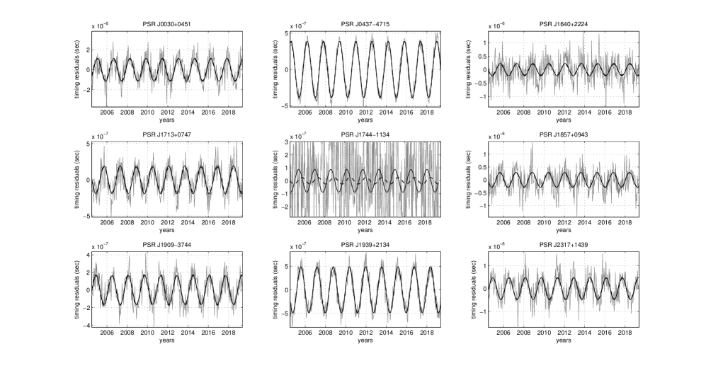
Figure 3: Data realization showing the simulated timing residuals (thin gray line) and signal (dash black line) for all pulsars. The network S/N $\rho_{n}=100$. The reconstructed signals are shown as solid curves. For most pulsars, except J1744–1134, the true and reconstructed signal are almost indistinguishable from each other. For PSR J1744–1134, we have zoomed into the noise so that the signal can be seen clearly.

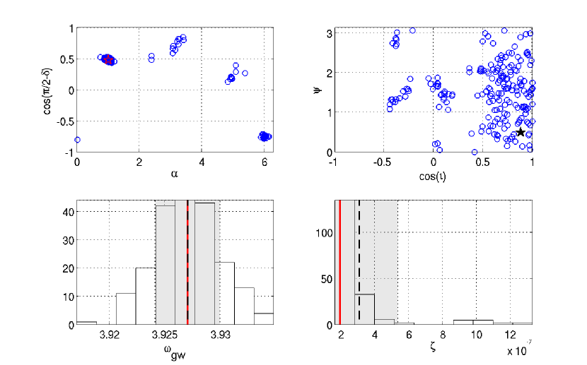
Figure 4: Two-dimensional scatter plots (top) and histograms (bottom) of estimated parameters for network S/N $\rho_{n}=100$. The star and the red vertical line mark the true values of the parameters. The dashed vertical line marks the mean value, and the shaded area covers the one-sigma region around the mean. The total number of trials is 200.

4.2 Moderate signal

Figure 5 shows a realization of the simulated data for a network S/N $\rho_{n}=30$. The noise is now seen to be stronger than the signal in most of the pulsars. The recovered signal continues to agree with the injected one quite well. Note that for PSR J1744–1134, J1713+0747 and J1640+2224, the deviation from the true signals is mainly in the amplitude, while the offset in phase is not significant. From the distribution of the detection statistic in Fig. 1, the detection probability is still practically unity for a detection threshold with an approximate false alarm probability of $2\times 10^{-3}$. In Figure 6, we see more clearly that the sky locations are centered on the same secondary maxima as in the $\rho_{n}=100$ case (Fig 4) but with an increased scatter around each. We also note that the bias in the estimation of the inclination and polarization angle is increased. The one-sigma uncertainties for $\omega_{\text{gw}}$ and $\zeta$ increase to $0.01~{}\text{rad}\cdot\text{yr}^{-1}$ and $8.63\times 10^{-7}~{}\text{sec}$, respectively. The increase in the errors is roughly consistent with their expected linear dependence on network S/N.

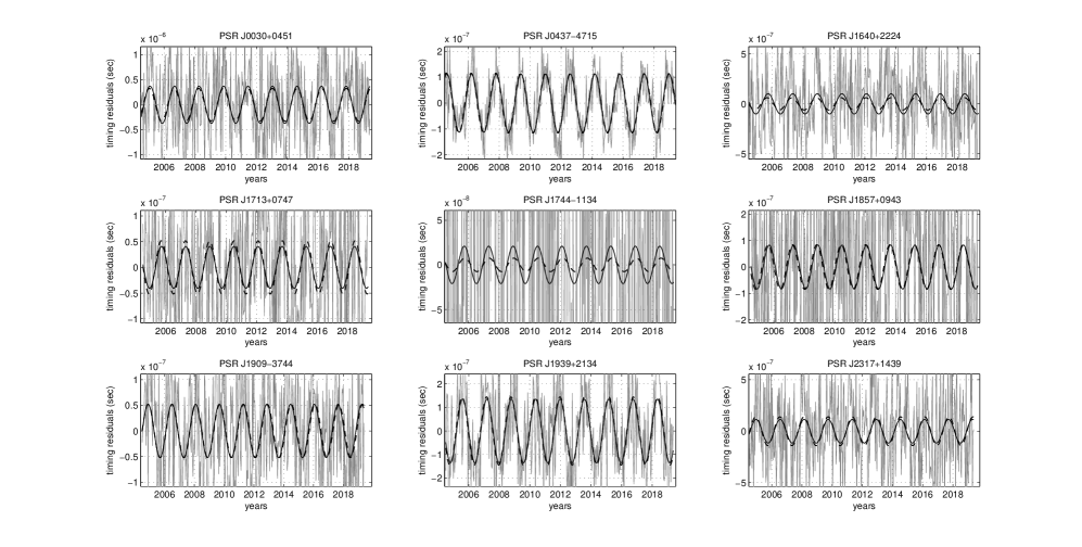
Figure 5: Data realization showing the simulated timing residuals (thin gray line) and signal (dash black line) for all pulsars. The network S/N is $\rho_{n}=30$. The reconstructed signals are shown as solid curves. For some pulsars, such as PSR J1744–1134 and J1857+0943, we have zoomed into the noise in the subplots, so that the signal can be seen clearly.

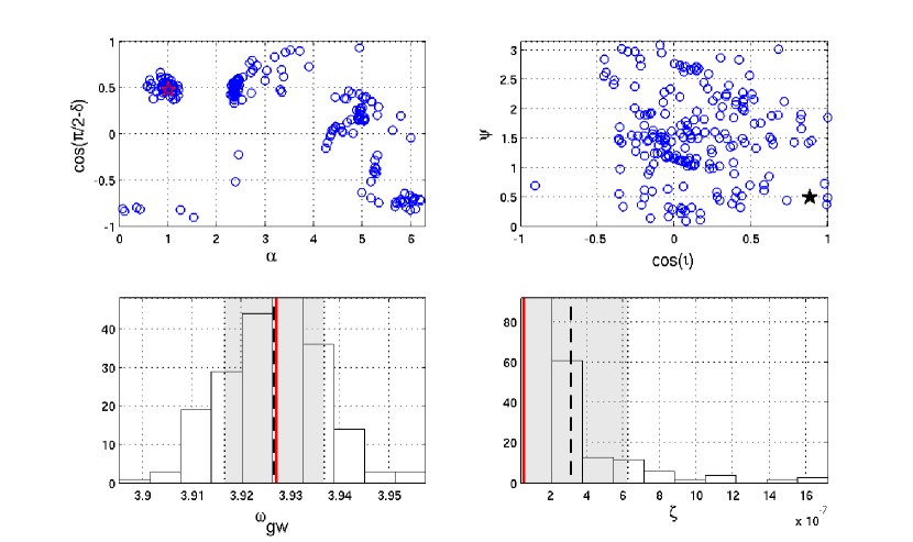
Figure 6: Two-dimensional scatter plots (top) and histograms (bottom) of estimated parameters for network S/N $\rho_{n}=30$. The star and the red vertical line mark the true values of the parameters. The dashed vertical line marks the mean value, and the shaded area covers the one-sigma region around the mean. The total number of trials is 200.

4.3 Weak signal

In this case, the network S/N $\rho_{n}=8$ corresponds to a weak and barely detectable signal. This is also the network S/N used in Taylor et al. (2014). Figure 7 shows one of the realizations of the simulated timing residuals. In this scenario, the noise dominates the signal in all pulsars. This illustrates the most likely situation with the current level of timing precision obtained in pulsar timing arrays. Even though the noise is loud, the recovered signals have deviations mainly in the amplitude (usually biased towards a larger value), while the offset in the phase is tolerable. In Figure 8, the scatter of the sky location becomes larger, but the presence of secondary maxima seen in the previous cases is still discernible. However, now the true location attracts the least number of trial values. The bias in the estimation of the inclination and polarization angle is now much clearer. The uncertainties in $\omega_{\text{gw}}$ and $\zeta$ are $0.036~{}\text{rad}\cdot\text{yr}^{-1}$ and $2.11\times 10^{-6}~{}\text{sec}$, again roughly consistent with the expected linear dependence on network S/N. From Figure 1, the detection probability is $Q_{d}\simeq 0.86$ if we choose the detection threshold to be the largest value of the noise-only distribution. In this case, the signal is still large enough to be detected, although it cannot be localized at all.

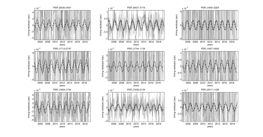
Figure 7: Data realization showing the simulated timing residuals (thin gray line) and signal (dash black line) for all pulsars. The network S/N is $\rho_{n}=8$. The reconstructed signals are shown as solid curves. For most pulsars, we have zoomed into the noise in the subplots, so that the signal can be manifested.

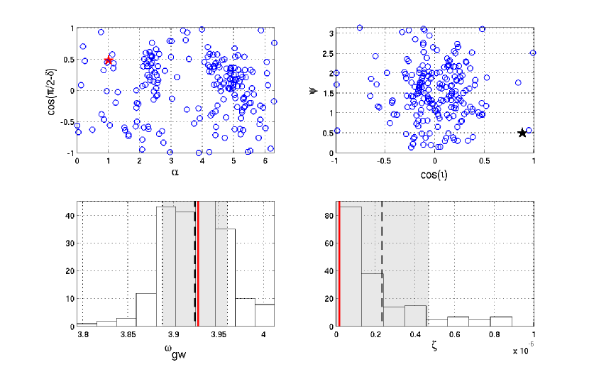
Figure 8: Two-dimensional scatter plots (top) and histograms (bottom) of estimated parameters for network S/N $\rho_{n}=8$. The star and the red vertical line mark the true values of the parameters. The dashed vertical line marks the mean value, and the shaded area covers the one-sigma region around the mean. The total number of trials is 200.

4.4 Comparison with other algorithms

In Figure 9, we show the log likelihood ratio from MaxPhase versus those from WMJ1 for a subset of 100 data realizations chosen randomly from the set used for the simulations reported above. We can see that for most realizations in each of the three signal strength scenarios, the former can find a marginally larger (better) log likelihood ratio than the latter, which suggests that MaxPhase can achieve a greater detection probability than WMJ1 for a given detection threshold.

Comparing parameter estimation performance, Figure 10 gives the estimated sky locations from WMJ1. For the $\rho_{n}=100$ case, the sky localization is very similar to the corresponding one in Figure 4, except that there are no secondary maxima. With the decreasing of $\rho_{n}$ to 30 and 8, the sky localization scatter increases but it still appears uni-modal and concentrated around the true value.

Comparing our results for MaxPhase and WMJ1 with those of the Bayesian method (Taylor et al., 2014), we make the following observations. From the receiver operating characteristics (ROC) curve reported in Fig. 6 of Taylor et al. (2014), the detection probability appears to be close to unity for $\rho_{n}=8$ case at the lowest false alarm probability of 0.01 used in that paper. The corresponding detection probability from MaxPhase is $97.5\%$ (and rapidly approaches unity for higher FAP). Thus, the detection performance of MaxPhase is comparable to that of the Bayesian method. The distribution of the estimated parameters in the Frequentist case can be compared more reliably with the distribution of the maximum-a-posteriori value of the parameters in the Bayesian method. We have picked the same source parameters as in Taylor et al. (2014), so the comparison is straightforward. Although there are differences between the two analyses, such as the use of irregularly versus regularly sampled data, they should not impact the comparison too much. From Figure 8 (MaxPhase), Figure 10 (WMJ1) in this paper and Figure 5 (Bayesian) in Taylor et al. (2014), we see that for $\rho_{n}=8$ case (the only case considered in Taylor et al. (2014)), the estimated sky location by MaxPhase is inferior to the Bayesian method, while the results from WMJ1 and the Bayesian method are qualitatively comparable.

Regarding computational costs, MaxPhase takes 6.7 min on average to complete one PSO run for each data realization on a single processor core, while the WMJ1 algorithm takes 89 min. As far as obtaining point estimates of the signal parameters is concerned, the reported computational cost of the Bayesian algorithm appears to be significantly higher than either of the Frequentist methods. For example, 48 cores are used in Taylor et al. (2014) to run a parallelized implementation of the MultiNest algorithm (Feroz et al., 2009) and the analysis is reported to typically take up to 45 minutes to complete at a network S/N $\rho_{n}=10$. However, it should be noted that the Bayesian method also maps out the posterior probability distribution of parameters, which may provide useful information in an analysis. Interestingly, it has been demonstrated in the context of CMB analysis that a fitting procedure may be combined with PSO to map out the likelihood function locally around the point estimate (Prasad & Souradeep, 2012). Thus, it may be possible to similarly extend MaxPhase (or WMJ1) to obtain information similar to that of a Bayesian method. This will lead to a corresponding increase in the computational cost of MaxPhase.

Figure 9: In each panel, Log likelihood ratio values from MaxPhase algorithm v.s. WMJ1 algorithm are shown for three scenarios with $\rho_{n}=100$, $30$, and $8$, respectively. The number of independent data realization is 100. In almost all trials, the log-likelihood ratios are seen to be higher for the MaxPhase algorithm.

Figure 10: In each panel, blue circles show the estimated sky locations for the source, which are obtained from the WMJ1 algorithm for a PTA consisted of 9 pulsars. A red star marks the true location of the source used in the simulation. The x-axis represents Right Ascension and the y-axis represents the declination. The total number of independent data realization is 100. The panel on the right may be compared with Fig. 5 of Taylor et al. (2014).

4.5 Effect of increasing the PTA size

As we noticed in the strong signal scenario, the maximization over the pulsar phases leaves behind a log-likelihood ratio that has strong secondary maxima, a feature that is absent if the pulsar phases are treated as intrinsic parameters. If these secondary maxima are comparable to the global maximum in value, they become attractors for stochastic search algorithms and reduce their effectiveness in locating the global maximum. With a decrease in signal-to-noise ratio, the probability of the locations of such secondary maxima becoming the global maximum increases. Both these effects worsen parameter estimation as we see in the moderate and weak signal cases.

This situation can be substentially improved by adding more pulsars in a PTA. Unlike the ground and space borne laser interferometers, adding more detectors (millisecond pulsars) in a PTA is technically easier and cheaper in terms of costs. Here, we demonstrate this by using the NANOGrav configuration (Demorest et al., 2013) which consists of 17 pulsars in the catalog. We keep the network S/N $\rho_{n}$ the same for each scenario as in the analysis reported in Sec. 4.1–4.4 with 9 pulsars. Accordingly, the overall amplitude $\zeta$ of the GW is scaled down. This implies that the signal amplitude for individual pulsars becomes significantly lower.

Fig. 11 presents the estimations of Right Ascension and declination of the GW source for 100 independent data realizations with $\rho_{n}=100$, 30 and 8 cases. Clearly, the scatter and the secondary maxima in the sky localization are effectively suppressed comparing to the ones in Fig. 4 and 6 for the strong and moderate signal cases. For the weak signal case, although the localization is still inferior compared to WMJ1 and the Bayesian algorithm, the bias appearing in Fig. 8 is gone and the distribution becomes quite uniform.

Figure 11: In each panel, blue circles show the estimated sky locations of the source, which are obtained from the MaxPhase algorithm for a PTA consisted of 17 pulsars. A red star marks the true location of the source used in the simulation. The x-axis represents Right Ascension and the y-axis represents the declination. The number of independent data realization is 100.

5 Summary and conclusions

Combined with WMJ1, this paper completes the first step in the program of implementing a purely Frequentist detection and parameter estimation approach for continuous wave GW signals using PTAs. There exists a dichotomy in how a GLRT can be implemented for this problem and this paper addresses the approach where pulsar phases are treated as extrinsic parameters that are maximized semi-analytically. Maximizing over pulsar phases is attractive compared to the alternative where they are treated as intrinsic parameters because the GLRT becomes scalable with the size of a PTA. The maximization over the pulsar phases leaves behind a 7-dimensional numerical optimization problem irrespective of the number of pulsars in a PTA. We find that the latter problem is effectively handled using PSO, as was the case in WMJ1, without requiring much tuning. Computational costs of PTA data analysis methods will become especially important for analyzing the IPTA data set that includes about 50 pulsars.

The approach based on the analytical maximization over pulsar phases has the merit that it does not involve the type of constrained maximization that appeared in WMJ1. This greatly simplifies the implementation and boosts the computation speed of the method. However, our results indicate that the performance of the method is not as good as far as estimation of the source location and some of the other angular parameters is concerned. The increased errors appear to stem from secondary maxima. The fact that these secondary maxima disappear when the PTA size is increased, suggests that they are likely to be the result of not taking the ill-posedness of the GW network analysis problem – well known in the context of ground based detector networks (Klimenko et al., 2005; Mohanty et al., 2006) – into account.

Mitigation of ill-posedness can be achieved by regularization of the inverse problem in some form (Greville, 1959; Tikhonov & Arsenin, 1977; Rakhmanov, 2006). However, unlike ground based networks of large-scale detectors, we have the simple option in the case of PTAs to increase the number of independent detectors (i.e., pulsars). In fact, the NANOGrav collaboration is adding 3-4 new MSPs, discovered from the ongoing major pulsar surveys at Arecibo Observatory and Green Bank Telescope (e.g., PALFA and GBNCC), in the observation campaign every year. As known for the ground-based case, this should reduce the effect of ill-posedness. That this is so is shown explicitly by taking a PTA with a larger number of pulsars. However, although increasing the number of pulsars is an obvious way to mitigate the problem of ill-posedness, the results for the weak signal case –the realistic one for the current PTAs– show that it cannot be completely ignored and must be addressed properly. We leave a deeper look at the problem of ill-posedness and regularization to future work.

The results reported here were obtained under the following limitations. The simulated data was evenly sampled whereas real data will have irregular sampling. However, our method works entirely in the time domain, and no major changes are needed to accommodate irregularly sampled data. In fact, if the irregularly sampled data have identically and independently distributed noise samples, no change in the algorithm is required. If, as some studies point out, the noise is not Gaussian or stationary, the actual covariance matrix for the given data will need to be modeled (or estimated) (Wang & et al., 2015; Wang, 2015). Regarding non-Gaussianity, it is worth noting that Finn (2001) shows that coherent techniques, such as MaxPhase and WMJ1, are generally robust against non-Gaussianity in the noise components.

The timing residuals for real data are obtained by fitting, using weighted least squares, a timing model to the data and subtracting it out. The timing model contains a set of parameters specific to the pulsar whose pulse arrival times are being fitted. The fitting procedure can affect the signal form as well as the statistics of the noise in the residual. When analyzing observational data, a common practice is to use the projection matrix R suggested by Demorest et al. (2013). A nice feature of R is that it only depends on the fitting model and the weighting matrix used, not the data itself. The influence of fitting can be easily taken into account by operating R on the timing residuals in the algorithm.

In constructing the GLRT, we assumed that the noise parameters are known a priori or can be estimated independently of the GW analysis. A more sophisticated approach would include the noise parameters as part of the estimation procedure. Since these additional parameters would be intrinsic in nature, directly including them in the GLRT would increase the search space dimensionality for PSO significantly. For example, the number of dimension increases from 7 to 52 for a PTA with 9 pulsars. Although such large dimensional optimization problems appear frequently in the PSO literature, it remains to be seen how the increase in dimensionality will pan out in the case of PTA data analysis. Some dimensional reduction scheme, of which fixing the noise model parameters a priori is an extreme example, will probably need to be implemented.

Finally, our signal model does not include the ellipticity or the evolution of binary orbit during the period of observation. However, these modifications will only lead to a few more intrinsic parameters that are specific to the GW signal and not associated with the pulsars. A study of the GLRT approach for more sophisticated signal models will be carried out in future works.

6 Acknowledgments

This work was supported by the National Science Foundation under PIRE grant 0968296. The contribution of S.D.M. to this paper is supported by NSF awards PHY-1205585 and HRD-0734800. Y.W. is supported by the National Science Fundation of China (NSFC) under grant NO. 11503007. We are grateful to the members in the NANOGrav for helpful comments and discussions. We thank the anonymous referees for helpful comments. Y. W. acknowledges the hospitality of School of Physics at the University of Western Australia during his visiting, where part of this work has been done.

References

- Arzoumanian et al. (2014) Arzoumanian, Z., Brazier, A., Burke-Spolaor, S., Chamberlin, S. J., Chatterjee, S., Cordes, J. M., Demorest, P. B., Deng, X., Dolch, T., Ellis, J. A., Ferdman, R. D., Finn, L. S., Garver-Daniels, N., Jenet, F., Jones, G., Kaspi, V. M., Koop, M., Lam, M., Lazio, T. J. W., Lommen, A. N., Lorimer, D. R., Luo, J., Lynch, R. S., Madison, D. R., McLaughlin, M., McWilliams, S. T., Nice, D. J., Palliyaguru, N., Pennucci, T. T., Ransom, S. M., Sesana, A., Siemens, X., Stairs, I. H., Stinebring, D. R., Stovall, K., Swiggum, J., Vallisneri, M., van Haasteren, R., Wang, Y., & Zhu, W. W. 2014, ArXiv e-prints
- Babak & Sesana (2012) Babak, S., & Sesana, A. 2012, Phys. Rev. D, 85, 044034
- Corbin & Cornish (2010) Corbin, V., & Cornish, N. J. 2010, ArXiv e-prints
- Cutler & Schutz (2005) Cutler, C., & Schutz, B. F. 2005, Phys. Rev. D, 72, 063006
- Degallaix et al. (2013) Degallaix, J., Accadia, T., Acernese, F., Agathos, M., Allocca, A., & et al. 2013, in Astronomical Society of the Pacific Conference Series, Vol. 467, 9th LISA Symposium, ed. G. Auger, P. Binétruy, & E. Plagnol, 151
- Demorest et al. (2013) Demorest, P. B., Ferdman, R. D., Gonzalez, M. E., Nice, D., Ransom, S., Stairs, I. H., Arzoumanian, Z., Brazier, A., Burke-Spolaor, S., Chamberlin, S. J., Cordes, J. M., Ellis, J., Finn, L. S., Freire, P., Giampanis, S., Jenet, F., Kaspi, V. M., Lazio, J., Lommen, A. N., McLaughlin, M., Palliyaguru, N., Perrodin, D., Shannon, R. M., Siemens, X., Stinebring, D., Swiggum, J., & Zhu, W. W. 2013, ApJ, 762, 94
- Deng & Finn (2011) Deng, X., & Finn, L. S. 2011, MNRAS, 414, 50
- Detweiler (1979) Detweiler, S. 1979, ApJ, 234, 1100
- Eberhart & Kennedy (1995) Eberhart, R., & Kennedy, J. 1995, in Micro Machine and Human Science, 1995. MHS’95., Proceedings of the Sixth International Symposium on, IEEE, 39–43
- Ellis (2013) Ellis, J. A. 2013, Classical and Quantum Gravity, 30, 224004
- Ellis et al. (2012) Ellis, J. A., Siemens, X., & Creighton, J. D. E. 2012, ApJ, 756, 175
- Feroz et al. (2009) Feroz, F., Gair, J. R., Hobson, M. P., & Porter, E. K. 2009, Classical and Quantum Gravity, 26, 215003
- Finn (2001) Finn, L. S. 2001, Phys. Rev. D, 63, 102001
- Foster & Backer (1990) Foster, R. S., & Backer, D. C. 1990, ApJ, 361, 300
- Greville (1959) Greville, T. N. E. 1959, SIAM Review, 1, 38
- Hellings & Downs (1983) Hellings, R. W., & Downs, G. S. 1983, ApJ, 265, L39
- Hobbs et al. (2014) Hobbs, G., Dai, S., Manchester, R. N., Shannon, R. M., Kerr, M., Lee, K. J., & Xu, R. 2014, ArXiv e-prints
- Jaffe & Backer (2003) Jaffe, A. H., & Backer, D. C. 2003, ApJ, 583, 616
- Jaranowski & Królak (2012) Jaranowski, P., & Królak, A. 2012, Living Reviews in Relativity, 15, 4
- Jaranowski et al. (1998) Jaranowski, P., Królak, A., & Schutz, B. F. 1998, Phys. Rev. D, 58, 063001
- Jenet et al. (2005) Jenet, F. A., Hobbs, G. B., Lee, K. J., & Manchester, R. N. 2005, ApJ, 625, L123
- Jenet et al. (2006) Jenet, F. A., Hobbs, G. B., van Straten, W., Manchester, R. N., Bailes, M., Verbiest, J. P. W., Edwards, R. T., Hotan, A. W., Sarkissian, J. M., & Ord, S. M. 2006, ApJ, 653, 1571
- Jenet et al. (2004) Jenet, F. A., Lommen, A., Larson, S. L., & Wen, L. 2004, ApJ, 606, 799
- Kay (1998) Kay, S. 1998, Fundamentals of Statistical Signal Processing, Volume II: Detection Theory (Prentice Hall)
- Klimenko et al. (2005) Klimenko, S., Mohanty, S., Rakhmanov, M., & Mitselmakher, G. 2005, Phys. Rev. D, 72, 122002
- Lee et al. (2011) Lee, K. J., Wex, N., Kramer, M., Stappers, B. W., Bassa, C. G., Janssen, G. H., Karuppusamy, R., & Smits, R. 2011, MNRAS, 414, 3251
- Lehmann (1959) Lehmann, E. L. 1959, Testing Statistical Hypotheses (New York: John Wiley)
- Lommen & Backer (2001) Lommen, A. N., & Backer, D. C. 2001, ApJ, 562, 297
- Manchester (2013) Manchester, R. N. 2013, Classical and Quantum Gravity, 30, 224010
- McLaughlin (2014) McLaughlin, M. A. 2014, ArXiv e-prints
- Mingarelli et al. (2012) Mingarelli, C. M. F., Grover, K., Sidery, T., Smith, R. J. E., & Vecchio, A. 2012, Physical Review Letters, 109, 081104
- Mohanty (2012a) Mohanty, S. D. 2012a, The Astronomical Review, 7, 020000
- Mohanty (2012b) —. 2012b, The Astronomical Review, 7, 040000
- Mohanty et al. (2006) Mohanty, S. D., Rakhmanov, M., Klimenko, S., & Mitselmakher, G. 2006, Classical and Quantum Gravity, 23, 4799
- Prasad & Souradeep (2012) Prasad, J., & Souradeep, T. 2012, Phys. Rev. D, 85, 123008
- Press et al. (2002) Press, W. H., Teukolsky, S. A., Vetterling, W. T., & Flannery, B. P. 2002, Numerical recipes in C++ : the art of scientific computing
- Rakhmanov (2006) Rakhmanov, M. 2006, Classical and Quantum Gravity, 23, 673
- Ravi et al. (2014) Ravi, V., Wyithe, J. S. B., Shannon, R. M., & Hobbs, G. 2014, ArXiv e-prints
- Romani & Taylor (1983) Romani, R. W., & Taylor, J. H. 1983, ApJ, 265, L35
- Sazhin (1978) Sazhin, M. V. 1978, Soviet Ast., 22, 36
- Seoane et al. (2013) Seoane, P. A., Aoudia, S., Audley, H., Auger, G., & et al. 2013, ArXiv e-prints
- Sesana & Vecchio (2010) Sesana, A., & Vecchio, A. 2010, Phys. Rev. D, 81, 104008
- Sesana et al. (2009) Sesana, A., Vecchio, A., & Volonteri, M. 2009, MNRAS, 394, 2255
- Seto (2009) Seto, N. 2009, MNRAS, 400, L38
- Shannon et al. (2013) Shannon, R. M., Ravi, V., Coles, W. A., Hobbs, G., Keith, M. J., Manchester, R. N., Wyithe, J. S. B., Bailes, M., Bhat, N. D. R., Burke-Spolaor, S., Khoo, J., Levin, Y., Oslowski, S., Sarkissian, J. M., van Straten, W., Verbiest, J. P. W., & Want, J.-B. 2013, Science, 342, 334
- Smits et al. (2009) Smits, R., Kramer, M., Stappers, B., Lorimer, D. R., Cordes, J., & Faulkner, A. 2009, A&A, 493, 1161
- Somiya (2012) Somiya, K. 2012, Classical and Quantum Gravity, 29, 124007
- Taylor et al. (2014) Taylor, S., Ellis, J., & Gair, J. 2014, Phys. Rev. D, 90, 104028
- Tikhonov & Arsenin (1977) Tikhonov, A. N., & Arsenin, V. Y. 1977, Solutions of Ill Posed Problems (Washington, D.C.: Vh Winston)
- van Haasteren et al. (2011) van Haasteren, R., Levin, Y., Janssen, G. H., Lazaridis, K., Kramer, M., Stappers, B. W., Desvignes, G., Purver, M. B., Lyne, A. G., Ferdman, R. D., Jessner, A., Cognard, I., Theureau, G., D’Amico, N., Possenti, A., Burgay, M., Corongiu, A., Hessels, J. W. T., Smits, R., & Verbiest, J. P. W. 2011, MNRAS, 414, 3117
- Waldman (2011) Waldman, S. J. 2011, ArXiv e-prints
- Wang (2015) Wang, Y. 2015, Journal of Physics Conference Series, 610, 012019
- Wang & et al. (2015) Wang, Y., & et al. 2015, to be submitted
- Wang & Mohanty (2010) Wang, Y., & Mohanty, S. D. 2010, Phys. Rev. D, 81, 063002
- Wang et al. (2014) Wang, Y., Mohanty, S. D., & Jenet, F. A. 2014, ApJ, 795, 96
- Wyithe & Loeb (2003) Wyithe, J. S. B., & Loeb, A. 2003, ApJ, 590, 691
- Yardley et al. (2011) Yardley, D. R. B., Coles, W. A., Hobbs, G. B., Verbiest, J. P. W., Manchester, R. N., van Straten, W., Jenet, F. A., Bailes, M., Bhat, N. D. R., Burke-Spolaor, S., Champion, D. J., Hotan, A. W., Oslowski, S., Reynolds, J. E., & Sarkissian, J. M. 2011, MNRAS, 414, 1777
- Yardley et al. (2010) Yardley, D. R. B., Hobbs, G. B., Jenet, F. A., Verbiest, J. P. W., Wen, Z. L., Manchester, R. N., Coles, W. A., van Straten, W., Bailes, M., Bhat, N. D. R., Burke-Spolaor, S., Champion, D. J., Hotan, A. W., & Sarkissian, J. M. 2010, MNRAS, 407, 669
- Zhu et al. (2014) Zhu, X.-J., Hobbs, G., Wen, L., Coles, W. A., Wang, J.-B., Shannon, R. M., Manchester, R. N., Bailes, M., Bhat, N. D. R., Burke-Spolaor, S., Dai, S., Keith, M. J., Kerr, M., Levin, Y., Madison, D. R., Osłowski, S., Ravi, V., Toomey, L., & van Straten, W. 2014, MNRAS, 444, 3709
- Zhu et al. (2015) Zhu, X.-J., Wen, L., Hobbs, G., Zhang, Y., Wang, Y., Madison, D. R., Manchester, R. N., Kerr, M., Rosado, P. A., & Wang, J.-B. 2015, MNRAS, 449, 1650