Phase evolution of the two-dimensional Kondo lattice model near half-filling

Abstract

Within a mean-field approximation, the ground state and finite temperature phase diagrams of the two-dimensional Kondo lattice model have been carefully studied as functions of the Kondo coupling $J$ and the conduction electron concentration $n_{c}$. In addition to the conventional hybridization between local moments and itinerant electrons, a staggered hybridization is proposed to characterize the interplay between the antiferromagnetism and the Kondo screening effect. As a result, a heavy fermion antiferromagnetic phase is obtained and separated from the pure antiferromagnetic ordered phase by a first-order Lifshitz phase transition, while a continuous phase transition exists between the heavy fermion antiferromagnetic phase and the Kondo paramagnetic phase. We have developed a efficient theory to calculate these phase boundaries. As $n_{c}$ decreases from the half-filling, the region of the heavy fermion antiferromagnetic phase shrinks and finally disappears at a critical point $n_{c}^{\ast}=0.8228$, leaving a first-order critical line between the pure antiferromagnetic phase and the Kondo paramagnetic phase for $n_{c}<n_{c}^{\ast}$. At half-filling limit, a finite temperature phase diagram is also determined on the Kondo coupling and temperature ($J$-$T$) plane. Notably, as the temperature is increased, the region of the heavy fermion antiferromagnetic phase is reduced continuously, and finally converges to a single point, together with the pure antiferromagnetic phase and the Kondo paramagnetic phase. The phase diagrams with such triple point may account for the observed phase transitions in related heavy fermion materials.

I Introduction

Since the discovery of heavy-fermion materials, the underlying mechanism controlling these rare earth or actinide-based compounds has continuously been the focuses of exploration Stewart01 ; Si01 ; Lohneysen07 . In these materials, the strong coupling limit of the on-site Kondo spin exchange causes the Kondo screening (KS) of local moments by the conduction electrons, yielding a Kondo paramagnetic (KP) phase. On the other hand, in the weak coupling limit, the Kondo coupling generates an indirect Ruderman-Kittel-Kasuya-Yosida interaction among the local moments, resulting in either antiferromagnetism (AFM) around the half-filling of the conduction electrons, or ferromagnetism (FM) far away from half-filling Doniach77 ; Lacroix79 .

However, in the intermediate Kondo coupling region, the competition between KS and magnetic correlation may produce a coexisting (CE) phase with AFM and KS near half-filling Zhang00 ; Paschen04 ; Friedemann09 ; Custers12 ; Isaev13 . The CE phase or so-called heavy fermion antiferromagnetic phase (HFAFM) has been observed in CeCoGe_3-xSi_x Duhwa98 ,and Ce₃Pd₂₀Si₆ Custers12 , etc. In Ce₃Pd₂₀Si₆, the HFAFM is observed within the magnetically ordered phase, indicating the separation of two transitions, i.e., the breakdown of Kondo screening effect and concomitant Fermi surface reconstruction (FSR) which happens between HFAFM and pure AFM, and the magnetic transition which occurs between HFAFM and KP phase Custers12 . However, studies of Hall coefficient and pressure effect in YbRh₂Si₂ have shown that the Kondo breakdown occurs precisely at the magnetic transition, while under Co and Ir doping, two transitions separate Paschen04 ; Friedemann09 ; Isaev13 . The Kondo breakdown also occurs away from the magnetic transition in CeIn₃ and CeRh_1-xCo_xIn₅ Harrison07 ; Goh08 .

To understand the novel behavior of the phase transitions in these materials, the corresponding parameter region and the feature of the AFM phase, CE phase, KP phase have been investigated within the framework of the Kondo lattice model (KLM) or Kondo Heisenberg lattice model, and intensively studied at zero temperature by mean-field approximation, variational Monte Carlo calculations, Gutzwiller approximation, etc Zhang00 ; Capponi01 ; Watanabe07 ; Martin08 ; Fabrizio08 ; Fabrizio13 . At half-filling limit, the reconstruction of the energy bands leads to an insulating state, and the ground state phases were computed with varying Kondo coupling Zhang00 ; Capponi01 ; Watanabe07 . Away from half-filling, the phase transitions are discussed by mean-field approximation on the Kondo Heisenberg lattice model, and the shift from onset to offset between the Kondo breakdown and magnetic transition is proposed to be driven by the change of the Heisenberg exchange and the ratio of short and long-range hopping strength Isaev13 .

Actually, the ground state phases and their features are controlled by the Kondo coupling $J$, the electron occupy number $n_{c}$ and the electron hopping strength. However, the phase evolutions with these parameters have not been fully explored yet, particularly how these phases evolute with $n_{c}$ and long-distance electron hoping remains an open issue Lacroix79 ; Fabrizio13 . In order to deal with this issue, we adopt the slave-fermion mean-field technique on the KLM, and developed a more efficient theory to calculate the phase boundaries between various phases. We show that the relative positions of Kondo breakdown and magnetic transition can be shifted by both $n_{c}$ and $t^{\prime}$ on the $n_{c}$-$J$ plane. As $n_{c}$ decreases, two transitions get closer and then coincide. This $n_{c}$-generating offset-to-onset structure with a triple point in the phase diagram is related to the experimental observations of Ce₃Pd₂₀Si₆ and YbRh₂Si₂ under doping.

On the other hand, most of earlier works focused on the ground state, while detailed theoretical studies at finite temperatures are still lacking. In the case when the occupation number of the conduction electron $n_{c}$ is far away from half-filling, the coexisting phase of FM and KS has investigated at finite temperatures and the phase diagram has been derived Zhang10 ; Liu13 . Remarkably, the boundaries separating the various phases joint to a single point on the $J$-$T$ plane, so an interesting issue arises as to whether the half-filled Kondo lattice system possesses similar feature in the finite temperature phase diagram. Therefore, we devote to study the ground state and finite-temperature phase diagram of the Kondo lattice model at and away from half-filling, attempting to give a detailed description of the evolution of the various phases with the Kondo coupling, the conduction electron occupy number, the electron hopping strength and temperature. To this end, a modified mean-field decoupling technique for the Kondo interaction is employed, then the phase diagrams are obtained as functions of $n_{c}$, $J$, $t^{\prime}$, and $T$ . Our method turns out to give a compact description of the phase diagrams at both zero and finite temperatures.

II Model and mean-field treatment

We consider the spin-1/2 Kondo lattice model on a two-dimensional square lattice with $N$ sites,

$$\mathcal{H}=\sum_{\mathbf{k},\sigma}(\epsilon_{\mathbf{k}}-\mu)c_{\mathbf{k}\sigma}^{{\dagger}}c_{\mathbf{k}\sigma}+J\sum_{i}\mathbf{S}_{i}\cdot\mathbf{S}_{ic},$$ (1)

where $\epsilon_{\mathbf{k}}$ is the dispersion of conduction electrons, which interact with local moments through antiferromagnetic Kondo exchange $J>0$, and $\mu$ denotes the chemical potential. $\mathbf{S}_{ic}=\frac{1}{2}\sum_{\alpha\beta}c_{i\alpha}^{{\dagger}}\bm{\sigma}_{\alpha\beta}c_{i\beta}$ with $\bm{\sigma}$ being the Pauli matrix, represents the spin density for conduction electrons, while the local moments can be written in the slave-fermion representation as $\mathbf{S}_{i}=\frac{1}{2}\sum_{\alpha\beta}f_{i\alpha}^{{\dagger}}\bm{\sigma}_{\alpha\beta}f_{i\beta}$, which is subject to the restriction $\sum_{\sigma}f_{i\sigma}^{{\dagger}}f_{i\sigma}=1$  imposing by a Lagrangian term $\sum_{i}\lambda_{i}(\sum_{\sigma}f_{i\sigma}^{{\dagger}}f_{i\sigma}-1)$. The Kondo interaction can be decomposed into

$$J\sum_{i}\mathbf{S}_{i}\cdot\mathbf{S}_{ic}= -\frac{3}{8}\sum_{i}(c_{i\uparrow}^{{\dagger}}f_{i\uparrow}+c_{i\downarrow}^{{\dagger}}f_{i\downarrow})(f_{i\uparrow}^{{\dagger}}c_{i\uparrow}+f_{i\downarrow}^{{\dagger}}c_{i\downarrow})$$

$$+\frac{1}{8}\sum_{i}(c_{i\uparrow}^{{\dagger}}f_{i\uparrow}-c_{i\downarrow}^{{\dagger}}f_{i\downarrow})(f_{i\uparrow}^{{\dagger}}c_{i\uparrow}-f_{i\downarrow}^{{\dagger}}c_{i\downarrow})$$

$$+\frac{1}{8}\sum_{i}(c_{i\uparrow}^{{\dagger}}f_{i\downarrow}+c_{i\downarrow}^{{\dagger}}f_{i\uparrow})(f_{i\downarrow}^{{\dagger}}c_{i\uparrow}+f_{i\uparrow}^{{\dagger}}c_{i\downarrow})$$

$$+\frac{1}{8}\sum_{i}(c_{i\uparrow}^{{\dagger}}f_{i\downarrow}-c_{i\downarrow}^{{\dagger}}f_{i\uparrow})(f_{i\downarrow}^{{\dagger}}c_{i\uparrow}-f_{i\uparrow}^{{\dagger}}c_{i\downarrow}),$$

where the first term represents the Kondo singlet screening effect and the other three terms describe the triplet parings between conduction electrons and slave fermion holes. This expression captures SU(2) invariance of the Kondo coupling.

In order to describe the antiferromagnetism in the Kondo lattice model, two AFM order parameters

$$m_{f}=\frac{1}{2}\sum_{\sigma}\sigma\langle f_{i\sigma}^{{\dagger}}f_{i\sigma}\rangle e^{i\mathbf{Q}\cdot\mathbf{R}_{i}},m_{c}=\frac{-1}{2}\sum_{\sigma}\sigma\langle c_{i\sigma}^{{\dagger}}c_{i\sigma}\rangle e^{i\mathbf{Q}\cdot\mathbf{R}_{i}}$$ (2)

are introduced to decouple the longitudinal Kondo spin exchange coupling Zhang00 , where $\mathbf{Q}=(\pi,\pi)$ is the AFM vector. Then the total staggered magnetization is expressed by $M=m_{f}-m_{c}$. To characterize the KS in the presence of AFM long-range ordering, two different hybridization parameters on each magnetic sublattice A and B have to be introduced Zhang00 ; Fabrizio13

$$V_{1}=\langle c_{iA\uparrow}^{{\dagger}}f_{iA\uparrow}\rangle=\langle c_{iB\downarrow}^{{\dagger}}f_{iB\downarrow}\rangle,$$

$$V_{2}=\langle c_{iB\uparrow}^{{\dagger}}f_{iB\uparrow}\rangle=\langle c_{iA\downarrow}^{{\dagger}}f_{iA\downarrow}\rangle.$$

The conventional hybridization parameter is expressed as

$$V_{s} = \frac{1}{2}(V_{1}+V_{2})$$

$$= \frac{1}{2}\langle c_{iA\uparrow}^{{\dagger}}f_{iA\uparrow}+c_{iA\downarrow}^{{\dagger}}f_{iA\downarrow}\rangle=\frac{1}{2}\langle c_{iB\uparrow}^{{\dagger}}f_{iB\uparrow}+c_{iB\downarrow}^{{\dagger}}f_{iB\downarrow}\rangle,$$

while the staggered hybridization parameter is defined by

$$V_{t} = \frac{1}{2}(V_{1}-V_{2})$$

$$= \frac{1}{2}\langle c_{iA\uparrow}^{{\dagger}}f_{iA\uparrow}-c_{iA\downarrow}^{{\dagger}}f_{iA\downarrow}\rangle=\frac{-1}{2}\langle c_{iB\uparrow}^{{\dagger}}f_{iB\uparrow}-c_{iB\downarrow}^{{\dagger}}f_{iB\downarrow}\rangle,$$

which requires the breaking of particle-hole symmetry of the conduction electrons, i.e., $n_{c}\neq 1$, or $t^{\prime}\neq 0$. It is seen that the singlet channel hybridizes the $c$- and $f$-fermions with the same wave vector, while the longitudinal exchange brings a momentum transfer $\mathbf{Q}$ within both $c$- and $f$-fermions, resulting in the staggered triplet channel. The local Lagrangian constraint is replaced by a uniform one: $\lambda_{i}=\lambda$.

Though such a mean-field treatment, the model Hamiltonian is written in the momentum space by the matrix form

$$\mathcal{H}=N\epsilon_{0}+{\sum_{\mathbf{k},\sigma}}^{\prime}\Phi_{\mathbf{k}\sigma}^{{\dagger}}\mathcal{H}_{\mathbf{k}\sigma}\Phi_{\mathbf{k}\sigma},$$ (3)

where the superscript represents the summation of $\mathbf{k}$ restricted in the magnetic Brillouin zone (MBZ) with boundaries $|k_{x}\pm k_{y}|=\pi$, a four-component Nambu operator has been used $\Phi_{\mathbf{k}\sigma}=(c_{\mathbf{k}\sigma}\hskip 2.84544ptc_{\mathbf{k}+\mathbf{Q}\sigma}\hskip 2.84544ptf_{\mathbf{k}\sigma}\hskip 2.84544ptf_{\mathbf{k}+\mathbf{Q}\sigma})^{T}$, and the constant term is given by $\epsilon_{0}=\frac{J}{2}(3V_{s}^{2}-V_{t}^{2})+Jm_{c}m_{f}-\lambda$. The Hamiltonian matrix is given by

$$\mathcal{H}_{\mathbf{k}\sigma}=\left(\begin{array}[]{cccc}\epsilon_{\mathbf{k}}-\mu&\frac{1}{2}Jm_{f}\sigma&-\frac{3}{4}JV_{s}&\frac{1}{4}JV_{t}\sigma\\ \frac{1}{2}Jm_{f}\sigma&\epsilon_{\mathbf{k}+\mathbf{Q}}-\mu&\frac{1}{4}JV_{t}\sigma&-\frac{3}{4}JV_{s}\\ -\frac{3}{4}JV_{s}&\frac{1}{4}JV_{t}\sigma&\lambda&-\frac{1}{2}Jm_{c}\sigma\\ \frac{1}{4}JV_{t}\sigma&-\frac{3}{4}JV_{s}&-\frac{1}{2}Jm_{c}\sigma&\lambda\end{array}\right),$$

where $\epsilon_{\mathbf{k}}=-2t(\cos{k_{x}}+\cos{k_{y}})+4t^{\prime}\cos{k_{x}}\cos{k_{y}}$ is the tight-binding dispersion of conduction electrons with nearest-neighbor (NN) and next-nearest-neighbor (NNN) hoping strength $t$ and $t^{\prime}$, respectively. In general filling case of conduction electrons, the quasiparticle excitation spectrums can not be derived analytically, we have to perform numerical calculations. However, at half-filling, the particle-hole symmetry can help to simplify the related calculations.

III Zero-temperature phase diagram at half-filling

We first discuss the half-filling limit with only NN hoping $t$. In this case, the particle-hole symmetry guarantees $\lambda=\mu=0$. Moreover, the staggered hybridization disappears as $V_{t}=0$. Further discussions including the influence of $n_{c}$ and NNN hoping $t^{\prime}$ will be given in the last section. The NN hoping between conducting electrons leads to the dispersion $\epsilon_{\mathbf{k}}=-2t(\cos{k_{x}}+\cos{k_{y}})$, satisfying the relation $\epsilon_{\mathbf{k}+\mathbf{Q}}=-\epsilon_{\mathbf{k}}$. For convenience, we define $V=-\frac{3}{2}V_{s}$, then the analytic formulas for the four dispersions are obtained by diagonalizing $\mathcal{H}_{\mathbf{k}\sigma}$:

$$\pm E_{\mathbf{k}}^{\pm}=\pm\frac{1}{\sqrt{2}}\sqrt{E_{1\mathbf{k}}\pm\sqrt{E_{1\mathbf{k}}^{2}-E_{2\mathbf{k}}^{2}}},$$ (4)

where

$$E_{1\mathbf{k}} =\epsilon_{\mathbf{k}}^{2}+\frac{1}{4}J^{2}(m_{c}^{2}+m_{f}^{2})+\frac{1}{2}J^{2}V^{2},$$

$$E_{2\mathbf{k}} =\sqrt{J^{2}m_{c}^{2}\epsilon_{\mathbf{k}}^{2}+\frac{1}{4}J^{4}(m_{c}m_{f}+V^{2})^{2}},$$

with the relation

$$E_{\mathbf{k}}^{-}+E_{\mathbf{k}}^{+}=\sqrt{E_{1\mathbf{k}}+E_{2\mathbf{k}}}\equiv E_{\mathbf{k}}.$$

At zero temperature, two lower branches of spectrums $-E_{\mathbf{k}}^{\pm}$ lying below the Fermi level are full occupied, giving rise to an insulating heavy fermion state. Two higher branches $E_{\mathbf{k}}^{\pm}$ above the Fermi level give no contribution to the ground state energy, therefore the ground state energy density is evaluated as

$$E_{g}^{CE}=[\frac{2}{3}JV^{2}+Jm_{c}m_{f}]-\frac{1}{N}{\sum_{\mathbf{k}}}E_{\mathbf{k}},$$ (5)

with the summation of $\mathbf{k}$ runs over the entire Brillouin zone. The mean-field order parameters are determined by minimizing $E_{g}^{CE}$, yielding the self-consistent equations

$$\frac{J}{4N}{\sum_{\mathbf{k}}}\frac{1}{E_{\mathbf{k}}}=\frac{m_{c}}{3(m_{f}-m_{c})},$$

$$\frac{J^{3}}{8N}(m_{c}m_{f}+V^{2}){\sum_{\mathbf{k}}}\frac{1}{E_{\mathbf{k}}E_{2\mathbf{k}}}=\frac{2m_{f}-3m_{c}}{3(m_{f}-m_{c})},$$

$$\frac{3J}{2N}{\sum_{\mathbf{k}}}\frac{\epsilon_{\mathbf{k}}^{2}}{E_{\mathbf{k}}E_{2\mathbf{k}}}=1+m_{f}/m_{c}.$$ (6)

In the whole coupling range, the pure AFM phase and KP phase should also be examined, then the stable ground state phase corresponds to the phase with lowest energy. When $m_{c}=m_{f}=0$, the energy density of KP phase is obtained by

$$E_{g}^{KP}=\frac{2}{3}JV^{2}-\frac{1}{N}\sum_{\mathbf{k}}\sqrt{\epsilon_{\mathbf{k}}^{2}+J^{2}V^{2}},$$ (7)

where $V$ is determined by $\frac{J}{N}\sum_{\mathbf{k}}\frac{1}{\sqrt{\epsilon_{\mathbf{k}}^{2}+J^{2}V^{2}}}=4/3$. For the pure AFM phase with $V=0$, the conduction electrons and the local moments are totally decoupled, resulting in the dispersions $E_{\mathbf{k}}^{\pm}=\pm\sqrt{\epsilon_{\mathbf{k}}^{2}+\frac{1}{4}J^{2}m_{f}^{2}}$ for the conduction electrons and $E_{d}^{\pm}=\pm\frac{1}{2}Jm_{c}$ for local moments, respectively. By performing similar self-consistent treatments, the energy for AFM phase is found to be

$$E_{g}^{AF}=-\frac{1}{N}\sum_{\mathbf{k}}\sqrt{\epsilon_{\mathbf{k}}^{2}+J^{2}/16},$$ (8)

with order parameters $m_{f}=1/2$, and $m_{c}=\frac{J}{8N}\sum_{\mathbf{k}}\frac{1}{\sqrt{\epsilon_{\mathbf{k}}^{2}+J^{2}/16}}$.

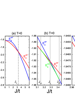
Figure 1: (Color online) (a) (b) Zero-temperature energies of AFM phase $E^{AF}_{g}$, KP phase $E^{KP}_{g}$ and CE phase $E^{CE}_{g}$ vs Kondo coupling $J$. (c) Free energies for the three phases as functions of $J$ at temperature $T=0.2t$. The CE phase exists in a narrow range between $J_{c1}$ and $J_{c2}$. All energies are in unit of NN hopping strength $t$.

The comparison of the ground state energies for AFM, CE and KP phases is demonstrated in Fig. 1(a)-(b). As expected, the competition between ordering of local moments and formation of Kondo singlets leads to a coexisting solution with lowest energy, indicating the stability of the CE phase in the intermediate Kondo coupling range $J_{c1}<J<J_{c2}$ Zhang00 , while the pure AFM phase and the KP phase exist in the region $J<J_{c1}$ and $J>J_{c2}$, respectively. The derived staggered magnetization $M=m_{f}-m_{c}$ and KS strength $V$ are given in Fig. 2(a) as a function of the Kondo coupling $J$. In the CE phase, the fluctuations of local spins in the Kondo channel suppress the AFM order, while the staggered magnetic order brings a rapid decrease of the KS strength. Both $M$ and $V$ vary continuously on the phase boundaries. $J_{c1}$ and $J_{c2}$ correspond to the lower boundary of the KS state with order parameters $m_{c}\neq 0,m_{f}\neq 0,V\rightarrow 0$, and the upper boundary of the AFM state with $m_{c}\rightarrow 0,m_{f}\rightarrow 0,V\neq 0$, respectively. The limit $V\rightarrow 0$ can be replaced by setting $V=0$ in the self-consistent equations Eq. (6), because the denominators of the integral functions are always nonzero, leading to the numerical results $J_{c1}=3.1498t,m_{f}=0.5,m_{c}=0.2735$. To calculate $J_{c2}$, we can simply set $m_{c}=0,m_{f}=0$ in the integrals in Eq. (6) because $E_{\mathbf{k}}=\sqrt{\epsilon_{\mathbf{k}}^{2}+J_{c2}^{2}V^{2}}$ and $E_{2\mathbf{k}}=\frac{1}{2}J_{c2}^{2}V^{2}$ are both gapped. To keep $m_{f}/m_{c}$ as a constant, we obtain the numerical solutions $J_{c2}=3.4161t,V=0.5853$.

As noticed, the energy of CE phase $E_{g}^{CE}$ is tangent to $E_{g}^{AF}$ on the edge $J_{c1}$, and to $E_{g}^{KP}$ at $J_{c2}$, respectively, implying that the Kondo lattice system undergoes second-order phase transitions on both phase boundaries. The coexistence of AFM and KS in the Kondo lattice systems has been reported previously at zero temperature Zhang00 ; Isaev13 ; Capponi01 . Though the proposed phase boundaries $J_{c1}$ and $J_{c2}$ are slightly different from our results, the main physical pictures remain the same. This inconsistence comes from distinct mean-field decoupling procedures. In these earlier studies, the Kondo exchange is decomposed directly into longitudinal term and transversal part (which is the singlet channel of hybridization), respectively; while in this work, the singlet and triplet hybridization between itinerant electrons and local moments are considered at the same level in the beginning. Therefore, our method can be generalized straightforwardly to deal with the case away from half-filling and with hoping beyond NN, as will be discussed in the following.

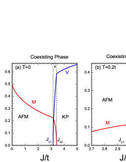
Figure 2: (Color online) Staggered magnetization $M$ and Kondo hybridization $V$ as functions of Kondo coupling $J$ at (a) $T$=0 and (b) $T$=0.2$t$ for the three phases.

IV Finite temperature phase diagram at half-filling

At finite temperatures, the existence of thermal fluctuations may shift the parameter region of the CE phase. For simplicity and without loss of generality, we consider half-filling case $n_{c}=1$ with $t^{\prime}=0$. Since in this situation, the mean-field Hamiltonian has been diagonalized with the spectrums $\pm E_{\mathbf{k}}^{\pm}$, the free energy density $F^{CE}$ can be calculated via the partition function, leading to the result

$$F^{CE}=\frac{2}{3}JV^{2}+Jm_{c}m_{f}-\frac{2T}{N}\sum_{\mathbf{k},\pm}\ln[2\cosh(E_{\mathbf{k}}^{\pm}/2T)].$$ (9)

It is easy to verify the equivalence of the ground state energy and above free energy at zero-temperature limit. The mean-field parameters are determined by minimizing $F^{CE}$, then the self-consistent equations are derived as

$$\frac{4}{3J}=\frac{1}{N}\sum_{\mathbf{k},\pm}F_{\mathbf{k}}^{\pm}[1\pm\frac{2E_{1\mathbf{k}}-J^{2}(m_{c}m_{f}+V^{2})}{2\sqrt{E_{1\mathbf{k}}^{2}-E_{2\mathbf{k}}^{2}}}],$$

$$\frac{2m_{c}}{J}=\frac{1}{N}\sum_{\mathbf{k},\pm}F_{\mathbf{k}}^{\pm}[m_{f}\pm\frac{2E_{1\mathbf{k}}m_{f}-J^{2}m_{c}(m_{c}m_{f}+V^{2})}{2\sqrt{E_{1\mathbf{k}}^{2}-E_{2\mathbf{k}}^{2}}}],$$

$$\frac{1}{N}\sum_{\mathbf{k},\pm}F_{\mathbf{k}}^{\pm}[m_{c}\pm\frac{E_{1\mathbf{k}}m_{c}-\frac{J^{2}}{2}m_{f}(m_{c}m_{f}+V^{2})-2m_{c}\epsilon_{\mathbf{k}}^{2}}{\sqrt{E_{1\mathbf{k}}^{2}-E_{2\mathbf{k}}^{2}}}]$$

$$=\frac{2m_{f}}{J}.$$ (10)

where $F_{\mathbf{k}}^{\pm}=\frac{1}{4E_{\mathbf{k}}^{\pm}}\tanh(E_{\mathbf{k}}^{\pm}/2T)$. In order to draw the phase diagram on the $J$-$T$ plane, the free energies of the pure AFM phase and KP phase should also be calculated.

The free energy of the KP phase is given by

$$F^{KP}=\frac{2}{3}JV^{2}-\frac{2T}{N}\sum_{\mathbf{k},\pm}\ln[2\cosh(E_{\mathbf{k}}^{\pm}/2T)],$$ (11)

with $E_{\mathbf{k}}^{\pm}=\frac{1}{\sqrt{2}}\sqrt{\epsilon_{\mathbf{k}}^{2}+J^{2}V^{2}/2\pm|\epsilon_{\mathbf{k}}|\sqrt{\epsilon_{\mathbf{k}}^{2}+J^{2}V^{2}}}$, and the equation for $V$:

$$\frac{4}{3J}=\frac{1}{4N}\sum_{\mathbf{k},\pm}\frac{\tanh(E_{\mathbf{k}}^{\pm}/2T)}{E_{\mathbf{k}}^{\pm}}(1\pm\frac{|\epsilon_{\mathbf{k}}|}{\sqrt{\epsilon_{\mathbf{k}}^{2}+J^{2}V^{2}}}).$$

As $T$ approaches Kondo temperature $T_{K}$, $V\rightarrow 0$, then $E_{\mathbf{k}}^{+}\rightarrow|\epsilon_{k}|$, $E_{\mathbf{k}}^{-}\rightarrow 0$, therefore $T_{K}$ of the KP phase is determined by

$$\frac{4}{3J}=\frac{1}{2N}\sum_{\mathbf{k}}\frac{\tanh(|\epsilon_{\mathbf{k}}|/2T_{K})}{|\epsilon_{\mathbf{k}}|}.$$ (12)

For the pure AFM phase, the corresponding free energy density is written as

$$F^{AF} =Jm_{c}m_{f}-2T\ln[2\cosh(E_{d}^{+}/2T)]$$

$$-\frac{2T}{N}\sum_{\mathbf{k}}\ln[2\cosh(E_{\mathbf{k}}^{+}/2T)],$$ (13)

with the self-consistent equations for the AFM order parameters:

$$m_{c}-\frac{Jm_{f}}{N}\sum_{\mathbf{k}}\frac{\tanh(E_{\mathbf{k}}^{+}/2T)}{4E_{\mathbf{k}}^{+}} =0,$$

$$m_{f}-\frac{1}{2}\tanh(Jm_{c}/4T) =0.$$

When $T$ approaches the Néel temperature $T_{N}$, $m_{f},m_{c}\rightarrow 0$, then $E_{\mathbf{k}}^{+}\rightarrow|\epsilon_{\mathbf{k}}|,E_{d}^{+}\rightarrow 0$, thus the equation determining $T_{N}$ is derived as

$$\frac{32T_{N}}{J^{2}}=\frac{1}{N}\sum_{\mathbf{k}}\frac{\tanh(|\epsilon_{\mathbf{k}}|/2T_{N})}{|\epsilon_{\mathbf{k}}|}.$$ (14)

In order to derive the finite-temperature phase diagram, the free energies of the AFM phase, the KP phase and the CE phase are compared. In Fig. 1(c), the free energies of the three phases are plotted as functions of kondo coupling strength $J$ at temperature $T=0.2t$. It can be seen that the CE phase is stable in the coupling range $J_{c1}<J<J_{c2}$, as it exhibits lowest free energy, and the AFM and KP phase occur in the coupling region $J<J_{c1}$ and $J>J_{c2}$, respectively. The phase boundaries $J_{c1}$ and $J_{c2}$ now vary with temperature, and are crucial to determine the phase diagram on the $J$-$T$ plane. Alternatively, we can consider the characteristic temperature separating CE phase with AFM phase as a function of $J$. On this boundary, $V$ approaches zero, so it appears as the Kondo temperature $T_{K}^{\prime}$ in CE phase. Using Eq. (10), the equations determining $T_{K}^{\prime}$ are reduced to

$$\frac{4}{3J}-\frac{1}{N}\sum_{\mathbf{k},\pm}\frac{\tanh(E_{\mathbf{k}}^{\pm}/2T_{K}^{\prime})}{4E_{\mathbf{k}}^{\pm}}[1\pm\frac{2E_{1\mathbf{k}}-J^{2}m_{c}m_{f}}{2\sqrt{E_{1\mathbf{k}}^{2}-E_{2\mathbf{k}}^{2}}}]=0,$$

$$\frac{m_{c}}{J}-\frac{m_{f}}{N}\sum_{\mathbf{k}}\frac{\tanh(E_{\mathbf{k}}^{+}/2T_{K}^{\prime})}{4E_{\mathbf{k}}^{+}}=0,$$

$$2m_{f}=\tanh(Jm_{c}/4T_{K}^{\prime}),$$ (15)

where $E_{1\mathbf{k}}=\epsilon_{\mathbf{k}}^{2}+\frac{1}{4}J^{2}(m_{c}^{2}+m_{f}^{2})$, $E_{2\mathbf{k}}=Jm_{c}\sqrt{\epsilon_{\mathbf{k}}^{2}+\frac{1}{4}J^{2}m_{f}^{2}}$, $E_{\mathbf{k}}^{+}=\sqrt{\epsilon_{\mathbf{k}}^{2}+J^{2}m_{f}^{2}/4}$, and $E_{\mathbf{k}}^{-}=Jm_{c}/2$.

On the boundary between CE phase and KP phase, the AFM order vanishes, so this phase boundary line corresponds to the Néel temperature $T_{N}^{\prime}$. On this edge, $m_{f}/m_{c}$ remains finite. The self-consistent equations determining $T_{N}^{\prime}$ with varying $J$ are simplified to

$$\frac{4}{3J}=\frac{1}{N}\sum_{\mathbf{k},\pm}\frac{\tanh(E_{\mathbf{k}}^{\pm}/2T_{N}^{\prime})}{4E_{\mathbf{k}}^{\pm}}[1\pm\frac{|\epsilon_{\mathbf{k}}|}{\sqrt{\epsilon_{\mathbf{k}}^{2}+J^{2}V^{2}}}],$$

$$\frac{2}{J}=\frac{1}{N}\sum_{\mathbf{k},\pm}\frac{\tanh(E_{\mathbf{k}}^{\pm}/2T_{N}^{\prime})}{4E_{\mathbf{k}}^{\pm}}[\gamma\pm\frac{2E_{1\mathbf{k}}\gamma-J^{2}V^{2}}{2\sqrt{E_{1\mathbf{k}}^{2}-E_{2\mathbf{k}}^{2}}}],$$

$$\frac{2\gamma}{J}=\frac{1}{N}\sum_{\mathbf{k},\pm}\frac{\tanh(E_{\mathbf{k}}^{\pm}/2T_{N}^{\prime})}{4E_{\mathbf{k}}^{\pm}}[1\pm\frac{E_{1\mathbf{k}}-\gamma J^{2}V^{2}/2-2\epsilon_{\mathbf{k}}^{2}}{\sqrt{E_{1\mathbf{k}}^{2}-E_{2\mathbf{k}}^{2}}}],$$ (16)

where $E_{1\mathbf{k}}=\epsilon_{\mathbf{k}}^{2}+J^{2}V^{2}/2$, $E_{2\mathbf{k}}=J^{2}V^{2}/2$, $E_{\mathbf{k}}^{\pm}=\frac{1}{\sqrt{2}}\sqrt{\epsilon_{\mathbf{k}}^{2}+J^{2}V^{2}/2\pm|\epsilon_{\mathbf{k}}|\sqrt{\epsilon_{\mathbf{k}}^{2}+J^{2}V^{2}}}$, and $\gamma=m_{f}/m_{c}$.

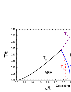
Figure 3: (Color online) Finite temperature phase diagram at half-filling. In addition to the pure AFM phase and KP phase, a coexisting phase emerges in the area between the lines $T^{\prime}_{K}$ and $T^{\prime}_{N}$. $T_{N}$ and $T_{K}$ are Néel temperature and Kondo temperature, respectively. Three phases converge to a single point on the $J$-$T$ plane.

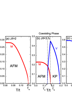
Figure 4: (Color online) Temperature dependence of staggered magnetization $M$ and KS strength $V$ at fixed Kondo couplings.

The critical lines $T_{K}$, $T_{N}$, $T_{K}^{\prime}$ and $T_{N}^{\prime}$ (which are all calculated as functions of $J$) necessary to determine the finite-temperature phase diagram at half-filling case are illustrated in Fig. 3. Both the Kondo temperature and Néel temperature show two distinct parts. In weak Kondo coupling region, the Néel temperature first increases from zero to a maximal value $T_{N}=0.238t$ at $J=2.85t$, then diminishes rapidly down to zero at a critical Kondo exchange $J_{c2}=3.4161t$. The reduction of $T_{N}$ in the intermediate coupling region is due to the spin fluctuations caused by the KS in the CE phase. For the Kondo temperature in the KP phase, it grows rapidly with increasing $J$ from $T_{K}=0.238t$ at $J=2.85t$ , while inside the CE phase, it shows a steep reduction down to zero from $J=2.85t$ to $J_{c1}=3.1498t$. The CE phase exists in the narrow region between $T_{K}^{\prime}$ and $T_{N}^{\prime}$, which contracts continuously as the temperature rises, then finally disappears.

Notably, the four lines intersect each other at $J=2.85t,T=0.238t$, showing that the AFM phase, the KP phase and the CE phase converge to a same point on the $J$-$T$ plane, similar to that reported in the case of far away from half-filling, where the ferromagnetism and KS coexist Zhang10 ; Liu13 . This feature of the phase diagram is similar to that derived by dynamic mean-field theory Si01 . In fact, the CE phase deduced by previous mean-field treatments Zhang00 ; Capponi01 does not converge together with the AFM and KP phase to a single point in the phase diagram, in contrast, the CE phase diminishes as temperature rises, and disappears inside the AFM and KP phase. Therefore, the existence of this convergent point deserves further verification beyond simple mean-field treatments.

The staggered magnetization $M$ and the Kondo hybridization parameter $V$ are calculated as a function of $J$ for given temperatures, illustrated in Fig. 2(b), and as functions of $T$ but constant $J$, demonstrated in Fig. 4. On the edge between AFM phase and CE phase (denoted by $J_{c1}$ in Fig. 2 and by $T_{K}^{\prime}$ in Fig. 4 (b)), $M$ varies continuously showing a kink, then decreases and approaches zero on the upper edge $J_{c2}$ or $T_{N}^{\prime}$; while on the boundary between CE phase and KP phase ($J_{c2}$ in Fig. 2 and $T_{N}^{\prime}$ in Fig. 4 (b)), the KS strength $V$ also varies continuously with a kink and then decreases and disappears when approaching the lower edge ($J_{c1}$ or $T_{K}^{\prime}$). The suppression of AFM order and Kondo hybridization by each other in CE phase is owing to the competition between them.

V Ground-state phase diagram close to half-filling

In above sections, the CE phase is studied in the half-filling case with only NN hoping $t$ among conduction electrons, and the systems is in an insulating phase. While away from half-filling or with NNN hoping $t^{\prime}$ or beyond, the system no longer possesses particle-hole symmetry, thus in addition to the singlet hybridization $V_{s}$, the triplet hybridization $V_{t}$ between the conduction electrons and local moments plays an important role. Consequently, the system may possess enriched phase transitions and phase diagram. In contrast to the mean-field methods in earlier works Zhang00 ; Capponi01 , the optimized mean-field decoupling we employed here can be naturally generalized to include the influence of $n_{c}$ and $t^{\prime}$, and various phases and phase transitions between them can be discussed explicitly.

In general case, the quasiparticle spectrums of CE phase have to be derived by diagonalizing $\mathcal{H}_{\mathbf{k}\sigma}$ numerically, and the unitary transformation between the quasiparticles and $c$ and $f$ fermions can also obtained through this computation. The six self-consistent equations for CE phase are derived by fitting the number of $c$ and $f$ fermions to $n_{c}$ and $1$, respectively, and by the definition of mean-filed parameters $V_{s}$, $V_{t}$, $m_{c}$, $m_{f}$. Each equation is expressed in turns of the matrix elements of the unitary transformation. These equations are solved iteratively until convergence is reached, then the energy of CE phase is obtained by summing the excitations below Fermi level. For pure AFM phase and KP phase, since the analytic spectrums exist, these two phase can be solved by minimizing their ground-state energies. In the AFM phase, the conduction electrons and $f$-fermions are decoupled, with $\lambda=0$, $m_{f}=1/2$, causing a smooth dispersions $E_{d}=\pm\frac{1}{2}Jm_{c}$ of local spins.

In order to determine the phase boundaries among the CE phase, AFM phase and KP phase, we have to develop an efficient theory. Considering when $J\rightarrow J_{c2}$, the parameters $m_{f},m_{c},V_{t}\rightarrow 0$, the quasiparticle spectrums of CE phase can be expressed by two parts: one is the function of $V_{s},\lambda,\mu$, and the other can be perturbed in the first-order of $m_{f},m_{c},V_{t}$. To do this, we rewrite the mean-field Hamiltonian to the form

$$\mathcal{H}=N\epsilon_{0}+{\sum_{\mathbf{k},\sigma}}^{\prime}\Phi_{\mathbf{k}\sigma}^{{\dagger}}\mathcal{H}_{\mathbf{k}\sigma}\Phi_{\mathbf{k}\sigma},$$ (17)

the operator are redefined as $\Phi_{\mathbf{k}\sigma}=(c_{\mathbf{k}\sigma}\hskip 2.84544ptf_{\mathbf{k}\sigma}\hskip 2.84544ptc_{\mathbf{k}+\mathbf{Q}\sigma}\hskip 2.84544ptf_{\mathbf{k}+\mathbf{Q}\sigma})^{T}$, and the Hamiltonian matrix

$$\mathcal{H}_{\mathbf{k}\sigma} =\left(\begin{array}[]{cccc}\epsilon_{\mathbf{k}}-\mu&-\frac{3}{4}JV_{s}&\frac{1}{2}Jm_{f}\sigma&\frac{1}{4}JV_{t}\sigma\\ -\frac{3}{4}JV_{s}&\lambda&\frac{1}{4}JV_{t}\sigma&-\frac{1}{2}Jm_{c}\sigma\\ \frac{1}{2}Jm_{f}\sigma&\frac{1}{4}JV_{t}\sigma&\epsilon_{\mathbf{k}+\mathbf{Q}}-\mu&-\frac{3}{4}JV_{s}\\ \frac{1}{4}JV_{t}\sigma&-\frac{1}{2}Jm_{c}\sigma&-\frac{3}{4}JV_{s}&\lambda\end{array}\right)$$

$$\equiv\left(\begin{array}[]{cc}A_{\mathbf{k}}&\sigma B_{\mathbf{k}}\\ \sigma B_{\mathbf{k}}&A_{\mathbf{k}+\mathbf{Q}}\end{array}\right).$$

Using the Bogoliubov transformation

$$\left(\begin{array}[]{c}c_{\mathbf{k}\sigma}\\ f_{\mathbf{k}\sigma}\end{array}\right)=U_{\mathbf{k}}\left(\begin{array}[]{c}\alpha_{\mathbf{k}\sigma}\\ \beta_{\mathbf{k}\sigma}\end{array}\right)=\left(\begin{array}[]{cc}u_{\mathbf{k}}&-v_{\mathbf{k}}\\ v_{\mathbf{k}}&u_{\mathbf{k}}\end{array}\right)\left(\begin{array}[]{c}\alpha_{\mathbf{k}\sigma}\\ \beta_{\mathbf{k}\sigma}\end{array}\right)$$

with $u_{\mathbf{k}}^{2}+v_{\mathbf{k}}^{2}=1$, the block diagonal parts $A_{\mathbf{k}}$ and $A_{\mathbf{k}+\mathbf{Q}}$ are diagonalized: $U_{\mathbf{k}}^{+}A_{\mathbf{k}}U_{\mathbf{k}}=\mathrm{diag}(E_{\mathbf{k}+}^{(0)},E_{\mathbf{k}-}^{(0)})\equiv\Lambda_{\mathbf{k}}$, $U_{\mathbf{k}+\mathbf{Q}}^{+}A_{\mathbf{k}+\mathbf{Q}}U_{\mathbf{k}+\mathbf{Q}}=\mathrm{diag}(E_{\mathbf{k}+\mathbf{Q}+}^{(0)},E_{\mathbf{k}+\mathbf{Q}-}^{(0)})\equiv\Lambda_{\mathbf{k}+\mathbf{Q}}$, where the dispersions are functions of $V_{s},\lambda,\mu$, and are equal to the spectrums in the KP phase:

$$E_{\mathbf{k}\pm}^{(0)}=\frac{1}{2}[\epsilon_{\mathbf{k}}-\mu+\lambda\pm\sqrt{(\epsilon_{\mathbf{k}}-\mu-\lambda)^{2}+9J^{2}V_{s}^{2}/4}].$$ (18)

To construct a global zero-order unitary transformation with Bogoliubov transformation

$$M_{\mathbf{k}}=\left(\begin{array}[]{cc}U_{\mathbf{k}}&0\\ 0&U_{\mathbf{k}+\mathbf{Q}}\end{array}\right),$$

which acts on the Hamiltonian matrix leads to

$$M_{\mathbf{k}}^{T}\mathcal{H}_{\mathbf{k}\sigma}M_{\mathbf{k}}=\left(\begin{array}[]{cc}\Lambda_{\mathbf{k}}&\sigma D_{\mathbf{k}}\\ \sigma D_{\mathbf{k}}^{T}&\Lambda_{\mathbf{k}+\mathbf{Q}}\end{array}\right).$$

The off-diagonal elements hybrid the zero-order eigenstates with each other, hence bring a correction to the dispersions: $E_{\mathbf{k}\pm}=E_{\mathbf{k}\pm}^{(0)}(V_{s},\lambda,\mu)+E_{\mathbf{k}\pm}^{(1)}(m_{c},m_{f},V_{t})$, where $E_{\mathbf{k}\pm}^{(1)}$ are easily obtained by these off-diagonal elements using perturbation theory. To the second order of $(m_{c},m_{f},V_{t})$, the ground-state energy density near $J_{c2}$ can be divided into two parts $E_{g}^{CE}=E_{g}^{(0)}(V_{s},\lambda,\mu)+E_{g}^{(1)}(m_{c},m_{f},V_{t})$, where

$$E_{g}^{(0)} =\frac{2}{N}\sum_{\mathbf{k},\pm}\theta(-E_{\mathbf{k}\pm}^{(0)})E_{\mathbf{k}\pm}^{(0)}+\frac{3}{2}JV_{s}^{2}-\lambda+\mu n_{c},$$

$$E_{g}^{(1)} =\frac{2}{N}\sum_{\mathbf{k},\pm}\theta(-E_{\mathbf{k}\pm}^{(0)})E_{\mathbf{k}\pm}^{(1)}-\frac{1}{2}JV_{t}^{2}+Jm_{c}m_{f}.$$ (19)

Minimization of $E_{g}^{(0)}$ with respect to $V_{s},\lambda,\mu$ gives rise to three self-consistent equations, while differentiating $E_{g}^{(1)}$ with $(m_{c},m_{f},V_{t})$ produces other three equations. At $J_{c2}$, $(m_{c},m_{f},V_{t})\rightarrow 0$, but $m_{f}/m_{c}$ and $V_{t}/m_{c}$ remain finite. Solving the six equations, $J_{c2}$ and the value of $V_{s}$, $\lambda$, $\mu$, $m_{f}/m_{c}$, $V_{t}/m_{c}$ on this boundary are calculated.

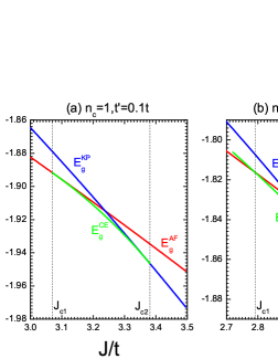
Figure 5: (Color online) Energies of AFM phase $E_{g}^{AF}$, KP phase $E_{g}^{KP}$ and CE phase $E_{g}^{CE}$ vs Kondo exchange $J$. All energies are in unit of NN hopping $t$.

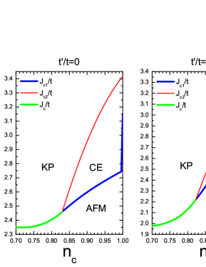
Figure 6: (Color online) Ground-state phase diagram of KLM near half-filling. As $n_{c}$ reduces, the collapse of KS at $J_{c1}$ and the magnetic transition at $J_{c2}$ get closer and finally converge. Thick and thin lines denote first and second order phase transitions, respectively.

In Fig. 5, the energies of the pure AFM phase, the CE phase and the KP phase are plotted with varying $J$, and the derived critical Kondo coupling $J_{c1}$ between AFM and CE phase on which the two phases have equal energy has been given as a function of $n_{c}$ and $t^{\prime}$ in Fig. 6. At half-filling, the pure AFM phase is separated with the CE phase by a second-order phase transition at $J_{c1}$, and on this boundary, $M$ varies continuously, while $V_{s}$ and $V_{t}$ approach zero, see Figs. 7(a). For $n_{c}<1$, the transition at $J_{c1}$ changes to a first-order one, as indicated by the kink in $E_{g}$ (Fig. 5(b)) and the discontinuity of $M$, $V_{s}$ and $V_{t}$ at $J_{c1}$ (Fig. 7(b)). Note that $V_{s}$ and $V_{t}$ remain finite at $J_{c1}$ for $n_{c}<1$. At $J_{c2}$, a second-order phase transition between CE and KP phase takes place, as seen by the tangency of ground state energy at $J_{c2}$ in Fig. 5. $E_{g}$, $V_{s}$, $V_{t}$, $M$ all vary continuously with $J$ at $J_{c2}$, at which $V_{t}$, $M$ approach zero. Moreover, the NNN hoping $t^{\prime}$ can shift both boundaries. We find a sudden jump of $J_{c1}$ at $n_{c}=1$ (see Fig. 6), this feature can be understood by the discontinuity of $M$ and $E_{g}^{CE}$ vs $n_{c}$ on $J_{c1}$ ( see Fig. 8) and may attribute to the change of topology, i.e., from the first order transition at $n_{c}<1$ to second-order transition at $n_{c}=1$. Only $J_{c2}$ represents a real phase transition, because at this boundary the staggered magnetization $M$ vanishes from AFM to KP phase.

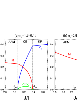
Figure 7: (Color online) Staggered magnetization $M$, Kondo hybridization $V_{s}$ and triplet hybridization $V_{t}$ as functions of Kondo coupling $J$.

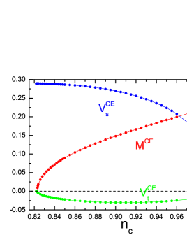
Figure 8: (Color online) Staggered magnetization $M$, Kondo hybridization $V_{s}$ and triplet hybridization $V_{t}$ on $J_{c1}$ as functions of $n_{c}$ for CE phase. At $n_{c}=1$, $V_{s}$ and $V_{t}$ approach zero (see Fig. 7a), while on the triple point ($n_{c}^{\ast}$=0.8228 for $t^{\prime}/t=0.1$), $M$ and $V_{t}$ disappear.

The spectrums and Fermi surface topological structures of these three phases are shown in Fig. 9. The itinerant electrons and local moments are completely decoupled in pure AFM phase, leading to a hole-like Fermi surface around $(\pi/2,\pi/2,)$ at $t^{\prime}=0.1$, which is consisted of the conduction electrons only and the Luttinger volume equals $n_{c}S_{F}$ , where $S_{F}$ is the area of Brillouin zone; while in the CE phase, the hybridization of conduction electrons and local moments constructs a hole-like Fermi surface around $(0,0)$ and $(\pi,\pi)$ points, with Fermi surface volume $n_{c}S_{F}$. The change of Fermi surface topology between AFM and CE phase indicates a first-order Lifshitz transition at $J_{c1}$. For the KP phase, a hole-like Fermi surface exists around $(\pi,\pi)$ with Fermi surface volume $\frac{1+n_{c}}{2}S_{F}$ containing both $c$- and $f$-fermions.

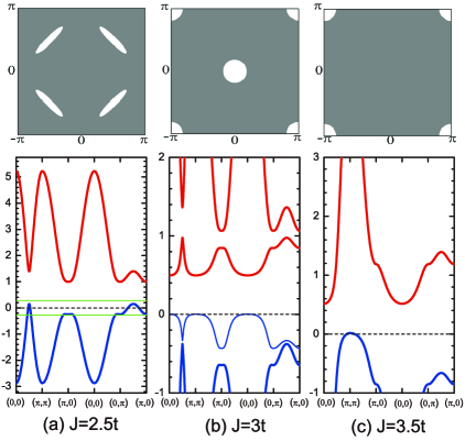
Figure 9: (Color online) Spectrums and Fermi surfaces of (a) AFM phase, (b) CE phase and (c) KP phase at $n_{c}=0.95$ and $t^{\prime}/t=0.1$. The shaded areas are the occupied Fermi sea, the white zones denote Fermi holes.

We have calculated $J_{c1}$ and $J_{c2}$ as $n_{c}$ varies from $0.7$ to $1$. Notably, as $n_{c}$ decreases, $J_{c1}$ and $J_{c2}$ approach each other and finally intersect at $n_{c}^{\ast}=0.8228,J^{\ast}=2.2181t$ for $t^{\prime}/t=0.1$, and at $n_{c}^{\ast}=0.8301,J^{\ast}=2.4604t$ for $t^{\prime}=0$, respectively. This result indicates that the CE phase region reduces with decreasing $n_{c}$ and finally disappears at a triple point. As $n_{c}$ decreases further, the AFM and KP phases are separated by a first-order transition at $J_{c}$, at which the AFM and KP phase shares equal energy. The ground state phase diagram of the KLM are summarized in Fig. 6 on the $n_{c}$-$J$ plane for given hopping parameter $t^{\prime}/t=0$ and $0.1$. When $n_{c}>n_{c}^{\ast}$, the collapse of $V_{s}$ at $J_{c1}$ and the magnetic transition occurring at $J_{c2}$ separate. While $n_{c}<n_{c}^{\ast}$, the KS collapses precisely at the magnetic transition point. Similar phase diagrams are also given by mean-field treatments, Gutzwiller approximation and variational Monte Carlo approach Isaev13 ; Fabrizio08 ; Watanabe07 . This offset-to-onset transition between Kondo breakdown and magnetic transition as $n_{c}$ decreases may account for the experimental observations for CeIn₃ and CeRh_1-xCo_xIn₅ Harrison07 ; Goh08 , and YbRh₂Si₂ under Co and Ir doping and external pressure Paschen04 ; Friedemann09 .

The triple point ($n_{c}^{\ast},J^{\ast}$) in our phase diagram can be shifted by $t^{\prime}/t$, so in our mechanism this offset-to-onset transition can also be generated by varying $t^{\prime}/t$, similar to that proposed in Ref. Isaev13 . Chemical or external pressure may simultaneously change $t^{\prime}/t$ and $n_{c}$, so which path cut in our phase diagram corresponding to these experiments is not clear. Experimental studies of the existence of $n_{c}^{\ast}$ may be particularly interesting. The KP phase possesses larger Fermi surface than AFM phases, consequently, the transition from AFM to KP at $J_{c}$ when $n_{c}<n_{c}^{\ast}$ may induce a abrupt change of Hall coefficient as in YbRh₂Si₂, where the FSR was observed via Hall effect at the onset of magnetic transition Friedemann09 .

VI Conclusion

In summary, we have performed an optimized mean-field decoupling of the Kondo lattice model near half-filling at both zero and finite temperatures. In addition to the pure AFM phase in weak Kondo coupling range and the Kondo paramagnetic phase in relatively strong coupling range, a distinct phase coexisting AFM order with Kondo hybridization arises in the intermediate Kondo exchange region, and the ground state phase diagram has been determined as function of the Kondo coupling, electron concentration and electron hopping. In particular, for the coexisting phase, we found a finite staggered triplet hybridization between local moments and conduction electrons. We also develop an efficient method to calculate the phase boundaries. The characteristic parameters and Fermi surface structures of these phases and the phase transitions between them have been discussed explicitly. We have further found a mechanism explaining the offset-to-onset transition between Kondo breakdown and magnetic transition, which is driven by the decreasing of electron number $n_{c}$. This mechanism may account for the separation of the two transitions in YbRh₂Si₂ under doping, and the existence of triple point ($n_{c}^{\ast},J^{\ast}$) in the phase diagram deserves deep experimental investigation. At half-filling limit, a finite-temperature phase diagram has been determined on $J$-$T$ plane. As temperature rises, the region of this coexisting phase diminishes continuously then finally converges to a single point, together with the pure AFM phase and KP phase, which may require further theoretical and experimental verification.

References

(1) G. Stewart, Rev. Mod. Phys. 73, 797 (2001).
(2) Qimiao Si, S. Rabello, K. Ingersent, and J. L. Smith, Nature
413, 804 (2001).
(3) H. V. Lohneysen, A. Rosch, M. Vojta, and P. Wolfle,
Rev. Mod. Phys. 79, 1015 (2007).
(4) S. Doniach, Physica B+C 91(0), 231 (1977).
(5) C. Lacroix and M. Cyrot, Phys. Rev. B 20, 1969
(1979).
(6) G. M. Zhang and L. Yu, Phys. Rev. B 62, 76 (2000).
(7) S. Paschen, T. Luhmann, S. Wirth, and P. Coleman, Nature
432, 881 (2004).
(8) S. Friedemann, T. Westerkamp, M. Brando, and F.
Steglich, Nature Physics 5, 465 (2009).
(9) J. Custers, K. A. Lorenzer, M. Müller et. al.,
Nature Materials 11, 189 (2012).
(10) L. Isaev and I. Vekhter, Phys. Rev. Lett. 110,
026403 (2013).
(11) E. Duhwa, Masavasu, K. Jiro, and T. Naova, J. Phys. Soc.
Jap 67, 2495 (1998).
(12) N. Harrison, S. E. Sebastian et. al., Phys. Rev. Lett.
99, 056401 (2007).
(13) S. K. Goh, J. Paglione et. al., Phys. Rev. Lett. 101, 056402 (2008).
(14) S. Capponi and F. F. Assaad, Phys. Rev. B 63,
155114 (2001).
(15) H. Watanabe and M. Ogata, Phys. Rev. Lett. 99,
136401 (2007).
(16) L. C. Martin and F. F. Assaad, Phys. Rev. Lett. 101, 066404 (2008).
(17) N. Lanatà, P. Barone, and M. Fabrizio, Phys. Rev. B
78, 155127 (2008).
(18) M. Z. Asadzadeh, F. Becca, and M. Fabrizio, Phys. Rev.
B 87, 205144 (2013).
(19) G. B. Li, G. M. Zhang, and L. Yu, Phys. Rev. B 81, 094420 (2010).
(20) Y. Liu, G. M. Zhang, and L. Yu, Phys. Rev. B 87,
134409 (2013).