On the stability and convergence of a class of consensus systems with a nonlinear input

Abstract

We consider a class of consensus systems driven by a nonlinear input. Such systems arise in a class of IoT applications. Our objective in this paper is to determine conditions under which a certain partially distributed system converges to a Lur’e-like scalar system, and to provide a rigorous proof of its stability. Conditions are derived for the non-uniform convergence and stability of such a system and an example is given of a speed advisory system where such a system arises in real engineering practice.

, , ,

1 Introduction

We consider nonlinear discrete-time systems described by

$$x(k+1)=P(k)x(k)+\mu\big{(}r-g(x(k))\big{)}e$$ (1)

where $k=0,1,2,\dots,$ $x(k)\in\mathbb{R}^{n}$, $P(k)$ is a $n\times n$ row stochastic matrix, $e=[1\ 1\,\dots\,1]^{T}\,$, $\mu$ and $r$ are scalars while $g$ is a scalar valued function. Equation (1) arises in consensus problems subject to an output constraint. It basically says that if consensus is achieved, it must be achieved subject to the equilibrium constraint $g(x^{*})=r$. That is, at equilibrium

$$g(x^{*})=r,$$ (2)

with $x_{i}^{*}=x_{j}^{*}$ for all $i,j\in\left\{1,2,...,n\right\}$. Equation (1) is of interest as it arises in many situations in the study of the internet of things (IOT). For example, in some situations a group of agents are asked to achieve a fair allocation of a constrained resource; TCP is an algorithm that strives to achieve this objective in internet congestion control. Recently, similar ideas have been applied in the context of the charging of electric vehicles, smart grid applications, and in the regulation of pollution in an urban context [19, 9]. A second application arises when one wishes to optimise an objective function subject to certain privacy constraints. For example, collaborative cruise control systems are emerging in which a group of vehicles on a stretch of road share information to determine a common speed that minimises fuel consumption of the group subject to some constraint (traffic flow, pollution constraints) [10]. Since each car is individually optimised for a potentially different speed, the technical challenge is for the group of cars to agree on a common speed without an individual revealing any of its inner workings to other vehicles. Other examples of this nature abound. As we have mentioned, for reasons of privacy, usually one does not attempt to solve such problems in a fully distributed manner. Neither, for reasons of robustness, scale, and communication overhead, does one attempt to solve them in a centralised manner. Rather, one uses a mix of local communication, and limited broadcast information, to solve these problem in a manner that conceals the private information of each of the individual agents. Implicit and explicit consensus algorithms that exploit local and global communication strategies are proposed and studied in [6, 7]. Equation (1) is perhaps the simplest algorithm of the explicit consensus algorithm with inputs, admitting a very simple intuitive understanding. It is well known that a row stochastic matrix $P$ operates on a vector $x\in\mathbb{R}^{n}$ such that $\textrm{max}(x)-\textrm{min}(x)\geq\textrm{max}(Px)-\textrm{min}(Px)$ where $\textrm{max}(x)$ and $\textrm{min}(x)$ are defined as the maximum and minimum component in vector $x$, respectively. Since the addition of $\big{(}r-g(x(k))\big{)}e$ does not affect this contraction, intuition suggests that $x_{i}(k)-x_{j}(k)\rightarrow 0$ as $k$ increases and eventually, the dynamics of (1) will be governed by the following scalar Lur’e system:

$$y(k+1)=y(k)+\mu(r\!-\!g(y(k)e)),$$ (3)

with $x_{i}(k)=y(k)$ asymptotically for all $i$. Intuition further suggests that, as long as (3) is stable, then so is (1). Arguments along these lines, in support of (1), are given in [6, 7]. However, these arguments are not complete in the sense that certain important properties are assumed to hold true. Our objective therefore in this brief note is to establish conditions on the function $g$ for which global uniform asymptotic stability is assured, and to rigorously prove the resulting assertions.

1.1 Comments on related literature

Before proceeding it is prudent to discuss connections to related work.

• (i) Cascade Systems : The setup we study can be viewed as a more general case of the systems studied in [13] where the authors prove local synchronization results for a general class of nonlinear time-varying systems. However, in contrast to the assumptions of that paper we do not require differentiability of the system maps and we state conditions which ensure global convergence. Further related work concerns stability analysis of nonlinear cascades [11, 12, 17]; we will comment on the relation to this literature in the system description and when stating results.
  

• (ii) Consensus : The setup we discuss is obviously connected to work on consensus. While the literature on consensus is too rich to give a complete survey here, recent surveys are available in [18, 14]. Here we briefly note that the standard problem studied in this literature are conditions that guarantee convergence of solutions to the consensus subspace. In this paper, we study the more specific problem of convergence to a specific point in which consensus is reached. Standard results ensuring consensus will therefore not apply in any classical sense to the problem studied here. Furthermore, a standard assumption in the case of a consensus system is a connectivity assumption on the communication graph. For a discussion of conditions used in this area we refer the reader to [15, 1, 14].
  

• (iii) Optimisation : As will be seen later, one particular application for the class of systems discussed in this paper allows for the solution of distributed optimisation problems using a consensus approach. While this is just one application of our result, and a minor part of this paper, some comments placing our work in this context are in order. Note, the idea to use consensus techniques to obtain approximations of optimal solutions has already been studied in other papers; see [16, 20, 3] for some work in this direction. For example, in [3], a constraint exchange based consensus algorithm was proposed, where the authors combined the ideas with dual decomposition and cutting-plane methods to solve convex and robust distributed optimisation problems via polyhedral approximations. While this approach is applicable to more general problems than those studied here, it is also more complex. Further, we note that many of the other techniques in the literature rely on the use of individual constraint sets for the agents and projections onto that set. These reduce to standard consensus in the case that no constraints are present.
  

• (iv) Convergence : As a further difference we point out that we give convergence results which can be non-uniform, whereas the authors in [16] point out that they rely on uniform convergence.

2 Notation, Conventions and Preliminary Results

2.1 Notation

We denote the standard basis in $\mathbb{R}^{n}$ by the vectors $e_{1},\ldots,e_{n}$. Note that $e=\sum_{i=1}^{n}e_{i}$. A matrix $P\in\mathbb{R}^{n\times n}$ is called row stochastic, if all its entries are nonnegative and if all its row sums equal one. The row sum condition is equivalent to $Pe=e$, that is, $e$ is an eigenvector of $P$ corresponding to the eigenvalue $1$. Hence there is a single transformation which achieves upper block triangularisation of all row stochastic matrices. Let $\{v_{2},\ldots,v_{n}\}$ be a basis for the $n-1$ dimensional subspace $e^{\perp}:=\{x\in\mathbb{R}^{n}\,:\,e^{T}x=0\}$. Then $\{e,v_{2},\ldots,v_{n}\}$ is a basis of $\mathbb{R}^{n}$. Consider now the transformation matrix $T:=\begin{bmatrix}e&v_{2}&\ldots&v_{n}\end{bmatrix}$ which represents a change of basis from the standard basis to the new basis. Under this transformation, a row stochastic matrix $P$ is transformed as follows:

$$T^{-1}PT=\begin{bmatrix}1&c\\ 0&Q\end{bmatrix}\,.$$ (4)

2.2 Facts about consensus

Given a sequence of row stochastic matrices $\{P(k)\}_{k\in\mathbb{N}}$, consider the time-varying linear system

$$x(k+1)=P(k)x(k)\,.$$ (5)

A solution of (5) is represented by the left products of the matrix sequence in the following sense: a sequence $\{x(k)\}_{k\in\mathbb{N}}$ is a solution of (5) corresponding to the initial condition $x(0)=x_{0}$ if and only if for all $k\in\mathbb{N}$,

$$x(k)=\Phi(k)x_{0}$$ (6)

where

$$\Phi(k):=P(k-1)\cdots P(0)\qquad\text{for all}\quad k\in\mathbb{N}\,.$$ (7)

The sequence $\{P(k)\}_{k\in\mathbb{N}}$ is called weakly ergodic if the difference between each pair of rows converges to zero, i.e. if for all $i,j$ we have

$$\lim_{k\to\infty}\left(e_{j}^{T}-e_{i}^{T}\right)\Phi(k)=0\,.$$ (8)

This is equivalent to system (5) being a consensus system, that is, every solution $\{x(k)\}_{k\in\mathbb{N}}$ of (5) satisfies

$$\lim_{k\to\infty}x_{j}(k)-x_{i}(k)=0$$ (9)

for all $i,j$. The sequence $\{P(k)\}_{k\in\mathbb{N}}$ is strongly ergodic if it is weakly ergodic and, in addition, the limit $\lim_{k\to\infty}\Phi(k)$ exists; we denote this limit by $\Phi_{\infty}$. Due to a result of Chatterjee and Seneta [4], weak and strong ergodicity are equivalent for left products of row stochastic matrices. This is equivalent to every solution of (5) satisfying

$$\lim_{k\to\infty}x(k)\in E\,,$$ (10)

or, equivalently,

$$\lim_{k\to\infty}\Phi(k)x_{0}\in E$$ (11)

for all $x_{0}\in\mathbb{R}^{n}$ where $E:=\operatorname{span}\{e\}$ is the space of consensus vectors. We call the sequence $\{P(k)\}_{k\in\mathbb{N}}$ strongly ergodic for all initial times, if all tail sequences $\{P(k)\}_{k=k_{0}}^{\infty}$ are strongly ergodic for all $k_{0}\in\mathbb{N}$. Note that a sequence can be strongly ergodic and not strongly ergodic for all initial times. For instance, if one of the matrices in the sequence has rank $1$ and all the subsequent matrices are the identity matrix. Using the transformation (4) a system equivalent to (5) is given by

$$\begin{array}[]{rcl}z(k+1)&=&T^{-1}P(k)Tz(k)\\ T^{-1}P(k)T&:=&\begin{bmatrix}1&c(k)\\ 0&Q(k)\end{bmatrix}\,.\end{array}$$ (12)

It is then clear that $\{P(k)\}$ is strongly ergodic if and only if

$$\lim_{k\to\infty}Q(k)\dots Q(0)=0\,.$$ (13)

A useful property in the study of products of row stochastic matrices is the observation that for any row stochastic matrix $P$ we have

$$\textrm{min}(x)\leq\textrm{min}(Px)\leq\textrm{max}(Px)\leq\textrm{max}(x)$$ (14)

for all $x\in\mathbb{R}^{n}$, where for any vector $y\in\mathbb{R}^{n}$,

$$\textrm{min}(y):=\textrm{min}\{y_{1},\dots,y_{n}\}\,,\ \textrm{max}(y):=\textrm{max}\{y_{1},\dots,y_{n}\}\,.$$

Introducing the function

$$V(x):=\textrm{max}(x)-\textrm{min}(x)\,,$$ (15)

(14) implies that $V(Px)\leq V(x)$. Also, the sequence $\{P(k)\}_{k\in\mathbb{N}}$ is strongly ergodic, if and only if

$$\lim_{k\rightarrow\infty}V\big{(}\Phi(k)x_{0}\big{)}=0$$ (16)

for all $x_{0}\in\mathbb{R}^{n}$ where $\Phi(k)$ is given by (7). Note that any vector $x\in\mathbb{R}^{n}$ can be uniquely decomposed as

$$x=\overline{x}e+x_{\perp}$$ (17)

where

$$\overline{x}:=(1/n)e^{T}x$$ (18)

is the mean of the components of $x$ and

$$x_{\perp}:=x-\overline{x}e\,,$$ (19)

Note that $\overline{x}e\in E$ and $e^{T}x_{\perp}=0$; hence

$$\operatorname{dist}(x,E)=\|x_{\perp}\|$$ (20)

where $\operatorname{dist}(x,E):=\inf\{\|x-z\|\,:z\in E\}\,$ is the distance of a vector $x\in\mathbb{R}^{n}$ to the consensus set $E$ and $\|x\|=\sqrt{x^{T}x}$.

Note also that

$$V(x)=V(x_{\perp})$$

and for any vector $z\in\mathbb{R}^{n}$ and any row-stochastic matrix $P\in\mathbb{R}^{n\times n}$ we have

$$\|z\|_{\infty}=\max_{1\leq i\leq n}|z_{i}|\quad\mbox{and}\quad\|P\|_{\infty}=\underset{1\leq i\leq n}{\text{max}}\sum\limits_{j=1}^{n}|P_{ij}|=1$$

where $P_{ij}$ is the entry in $i^{\textrm{th}}$  row and $j^{\textrm{th}}$  column of the matrix $P$.

As the following results rely on the existence of strongly ergodic sequences, it is of course of interest to have criteria for the occurrence of such a sequence. This is discussed extensively in the literature and here we can only discuss a limited number of references. A number of such criteria can be found in [4]. Relations of this notion to ergodicity or the Dobrushin coefficient is discussed in [5] and the references given therein. In addition, in the consensus literature there are numerous results on the convergence of iterated averaging, see e.g. [1, Theorem 1], and the survey given in [18, Section III].

3 Consensus under Feedback

Consider a sequence of row stochastic matrices $\{P(k)\}_{k\in\mathbb{N}}$ and a continuous function $G:\mathbb{R}^{n}\to\mathbb{R}$. Then the system,

$$\begin{array}[]{rcl}x(k+1)&=&F(k,x(k))\\ F(k,x)&:=&P(k)x+G(x)e\end{array}$$ (21)

can be regarded as a consensus system under feedback. In later statements, further differentiability assumptions will be imposed on $G$ as required. If we apply the similarity transformation defined in (4), then in the new coordinates, $y\in\mathbb{R},z\in\mathbb{R}^{n-1}$, given by $x=T[y\,\,z^{T}]^{T}$, we obtain

$$y(k+1) =y(k)+G(T[y(k)\,z(k)^{T}]^{T})+c(k)z(k)$$

$$z(k+1) =Q(k)z(k)\,.$$ (22)

The class of cascaded systems studied in [11, 12, 17] encompasses this system formulation. We note that in all these references and in subsequent literature based on these papers [8], it is assumed that the subsystems are globally uniformly asymptotically stable. We do not require this assumption. Associated with (21) we consider the one-dimensional system

$$\begin{array}[]{rcl}y(k+1)&=&h(y(k))\\ h(y)&:=&y+G(ye)\,,\end{array}$$ (23)

which is seen to be the one dimensional subsystem in the cascade (22) corresponding to $z(k)=0$. This is the aforementioned Lur’e system and, as we shall see, the dynamics of the consensus system (21) is strongly related to the dynamics of (23). Unless stated otherwise we consider the systems (21) and (23) with initial time $k_{0}=0$. A few comments on results that hold uniformly with respect to all initial times are made where appropriate.

3.1 Local Stability Results

Lemma 1.

Let $\{P(k)\}_{k\in\mathbb{N}}$ be a sequence of row stochastic matrices and $G:\mathbb{R}^{n}\to\mathbb{R}$. If $\{y(k)\}_{k\in\mathbb{N}}$ is a solution of (23) then $\{y(k)e\}_{k\in\mathbb{N}}$ is a solution of (21).

Proof 3.1.

This follows from $P(k)e=e$.

The next result tells us that the consensus system under feedback (21) is also a consensus system. We omit the straightforward proof of this observation.

Lemma 2.

If $\{P(k)\}_{k\in\mathbb{N}}$ is a strongly ergodic sequence of row stochastic matrices, then for every solution $\{x(k)\}_{k\in\mathbb{N}}$ of (21) we have

$$\lim_{k\to\infty}\operatorname{dist}\left(x(k),E\right)=0\,.$$ (24)

We now consider the local stability of (21) and see that it is determined by the stability of the induced system (23) on the consensus space. As we have no global concerns no Lipschitz property of $G$ is required. Initially, it is sufficient that $G$ be continuous.

Theorem 3.

Let $\{P(k)\}_{k\in\mathbb{N}}$ be a strongly ergodic sequence of row stochastic matrices and $G:\mathbb{R}^{n}\rightarrow\mathbb{R}$ be continuous. Suppose that $y^{\ast}$ is a locally asymptotically stable fixed point of the one dimensional system (23). Then $y^{\ast}e$ is a locally asymptotically stable fixed point at time $k_{0}=0$ for (21).

If the sequence $\{P(k)\}_{k\in\mathbb{N}}$ is strongly ergodic for all initial times, then $y^{\ast}e$ is asymptotically stable for all initial times $k_{0}\in\mathbb{N}$.

Proof 3.2.

Suppose that $y^{\ast}$ is a locally asymptotically stable fixed point for system (23). Let $W$ be a local Lyapunov function which guarantees this stability property. That is, $W(y^{*})=0$ and there is an open neighborhood $U$ of $y^{*}$ such that $W(y)>0$ and $W(h(y))<W(y)$ for all $y\in U\setminus\{y^{*}\}$. Without loss of generality we may assume $U$ to be a forward invariant set of (23), i.e., if $y\in U$ then $h(y)\in U$. For $\varepsilon>0$ such that $W^{-1}([0,\varepsilon])\subset U$ is a compact set we may choose $\delta>0$ sufficiently small, so that

$$W(h(y)+d)<\varepsilon\qquad\mbox{for}\qquad W(y)<\epsilon\quad\mbox{and}\quad|d|\leq\delta\,.$$

This is possible by continuity of all the functions involved and by the decay property of the Lyapunov function $W$.

We note that for any $x\in\mathbb{R}^{n}$, $Px=P(\overline{x}e+x_{\perp})=\overline{x}e+Px_{\perp}$, where $\bar{x}$ was defined as the mean of the entries of $x\in\mathbb{R}^{n}$ (recall from (18)). Hence

$$\overline{Px}-\overline{x}=\overline{x}+\overline{Px_{\perp}}-\overline{x}=(1/n)e^{T}Px_{\perp}\,.$$ (25)

Given a sufficiently small $\varepsilon>0$ and an appropriate $\delta$ as above, choosing $\eta>0$ such that $V(x)\leq\eta$ and $W(\bar{x})\leq\epsilon$ implies that for any row stochastic matrix $P$

$$|\overline{Px}-\overline{x}|+|G(x)-G(\overline{x}e)|<\delta\,.$$

This is possible by the estimate for

$$\|Px-x\|_{\infty}=\|Px_{\perp}-x_{\perp}\|_{\infty}\leq\|Px_{\perp}\|_{\infty}+\|x_{\perp}\|_{\infty}\leq 2\|x_{\perp}\|_{\infty}$$

and by uniform continuity of $G$ on a bounded neighborhood of $y^{*}e$. Consider now the neighborhood of $y^{*}e$ given by

$$N_{\varepsilon}:=\{x\in\mathbb{R}^{n}\,:\,\overline{x}\in U,\,W(\overline{x})<\varepsilon,V(x)<\eta\}\,.$$

We claim that $N_{\varepsilon}$ is forward invariant at all times $k\in\mathbb{N}$. Indeed, if $x(k)\in N_{\varepsilon}$, then we obtain

$$\overline{x}(k+1) =\overline{P(k)x(k)}+G(x(k))$$

$$=\overline{x}(k)+G(\overline{x}(k)e)+d$$

$$=h(\overline{x}(k))+d$$

where $d=\overline{P(k)x(k)}-\overline{x}(k)+G(x(k))-G(\overline{x}(k)e)$. Hence $|d|<\delta$ from which it follows that $W(\overline{x}(k+1))<\varepsilon.$ Referring to the argument in the proof of Lemma 2

$$V(x(k+1))=V(P(k)x(k))\leq V(x(k))<\eta.$$

As $\varepsilon,\eta$ were arbitrary, this shows stability of $y^{*}e$. To show local attractivity, let $x_{0}\in N_{\varepsilon}$ for $\varepsilon>0$ sufficiently small so that stability holds. Note that by Lemma 2 and by stability we have that $\omega(x_{0})\subset Ue\subset E$ where $\omega(x_{0})$ is the $\omega$-limit set of the solution corresponding to $x_{0}$ and $Ue:=\left\{ye:y\in U\right\}$ is a subset of $E$. Suppose that $ye\in\omega(x_{0})$ and $y\neq y^{*}$ . Then as the trajectory starting in $ye$ converges to $y^{*}e$ it follows that $y^{*}e\in\omega(x_{0})$. However, the assumption that $y^{*}e$ and $ye$ are in the $\omega$-limit set contradicts the stability of $y^{*}e$. Hence $\{x(k)\}_{k\in\mathbb{N}}$ converges to $y^{*}e$.

We now extend the previous result to local exponential stability. To this end we call a sequence of row stochastic matrices $\{P(k)\}_{k\in\mathbb{N}}$ exponentially ergodic if it is strongly ergodic and there exist scalars $M\geq 1$, $0<r<1$ such that for all $k\in\mathbb{N}$

$$\|\Phi(k)-\Phi_{\infty}\|\leq Mr^{k}\,.$$

The sequence is called uniformly exponentially ergodic, if it is strongly ergodic for all initial times and there exists constants $M,r$ so that for all $k_{0}\in\mathbb{N}$ there exists a matrix $\Phi_{\infty}$ so that for all $k>k_{0}$ we have $\|\tilde{\Phi}(k,k_{0})-\Phi_{\infty}\|\leq Mr^{(k-k_{0})}$; where $\tilde{\Phi}(k,k_{0}):=P(k-1)\cdots P(k_{0})$.

Theorem 4.

Let $\{P(k)\}_{k\in\mathbb{N}}$ be an exponentially ergodic sequence of row stochastic matrices and $G:\mathbb{R}^{n}\rightarrow\mathbb{R}$ be continuously differentiable. Suppose that $y^{\ast}$ is a locally exponentially stable fixed point of the one dimensional system (23). Then, $y^{\ast}e$ is a locally exponentially stable fixed point at time $k_{0}=0$ for (21). If the sequence $\{P(k)\}_{k\in\mathbb{N}}$ is uniformly exponentially ergodic, then $y^{\ast}e$ is locally uniformly exponentially stable.

Proof 3.3.

Consider the linearisation of the one-dimensional map defining (23). By the assumption of exponential stability it must satisfy

$$|h^{\prime}(y^{*})|<1$$ (26)

where $h^{\prime}(y^{*})=1+DG(y^{*}e)e$ and $DG$ is the derivative of $G$, which we interpret as a row vector. We now compute the derivative of $F$ with respect to $x$ at $x=y^{*}e$ and time $k$ to obtain

$$\frac{\partial F}{\partial x}(k,y^{*}e)=P(k)+eDG(y^{*}e).$$ (27)

If we now consider the transformation $T$ which results in (12) and using $T^{-1}e=e_{1}$ we see that

$$T^{-1}\frac{\partial F}{\partial x}(k,y^{*}e)T=\begin{bmatrix}1&c(k)\\ 0&Q(k)\end{bmatrix}+e_{1}DG(y^{*}e)T\,.$$ (28)

Two things are noticeable when considering this equation. First the resulting transformed matrix is of the form

$$\begin{bmatrix}\lambda&\tilde{c}(k)\\ 0&Q(k)\end{bmatrix}\,,$$ (29)

where only the first row is affected by $G$ and $\lambda$ is independent of $k$. Secondly,

$$\lambda=1+DG(y^{*}e)e=h^{\prime}(y^{*})\,.$$ (30)

Hence $|\lambda|<1$. By assumption $\|Q(k)Q(k-1)\dots Q(0)\|\leq Mr^{k}$ for suitable constants $M\geq 1$ and $r\in(0,1)$. It now follows that the linearised system of (21) at the fixed point $y^{*}e$ is exponentially stable. It follows by standard linearisation theory that the nonlinear system is locally exponentially stable at $y^{*}e$. If the sequence $Q(k)Q(k-1)\dots Q(0)$ converges to zero uniformly exponentially, this shows local uniform exponential stability of $y^{*}e$ for the nonlinear system.

3.2 Global Stability Results

To obtain global stability results we first need the following boundedness result.

Lemma 5.

Let $\{P(k)\}_{k\in\mathbb{N}}$ be a strongly ergodic sequence of row stochastic matrices and suppose that $G:\mathbb{R}^{n}\rightarrow\mathbb{R}$ is continuous and satisfies the following conditions.

• There exists an $\varepsilon>0$ such that $G$ satisfies a Lipschitz condition with constant $L>0$ on the set

  $$B_{\varepsilon}(E):=\{x\in\mathbb{R}^{n}\,:\,\operatorname{dist}(x,E)\leq\varepsilon\}\,.$$

• There exist constants $\beta,\gamma>0$ such that

  $$|h(y)|\leq|y|-\gamma\qquad\mbox{when}\quad|y|\geq\beta$$

  where $h(y)=y+G(ye)$.

Then every trajectory of (21) is bounded.

Proof 3.4.

Consider any solution $\{x(k)\}_{k\in\mathbb{N}}$ of (21) with $x(0)=x_{0}$. By Lemma 2 there exists a $k_{0}\in\mathbb{N}$ such that $x(k)\in B_{\varepsilon}(E)$ for all $k\geq k_{0}$. We can express $x(k)$ as $x(k)=\overline{x}(k)e+x_{\perp}(k)$ where $\overline{x}(k)=(1/n)e^{T}x(k)~{}\mbox{and}~{}x_{\perp}(k):=x(k)-\bar{x}(k)e.$ It follows from (24) that $\lim_{k\to\infty}\|x_{\perp}(k)\|=0.$ Hence boundedness of the sequence $\{\bar{x}(k)\}_{k\in\mathbb{N}}$ implies boundedness of $\{x(k)\}_{k\in\mathbb{N}}$. Considering the evolution of $\overline{x}(k)$ we obtain that, for $k\geq k_{0}$,

$$|\overline{x}(k+1)| = |\overline{P(k)x(k)}+G\big{(}\overline{x}(k)e+x_{\perp}(k)\big{)}|$$

$$\leq |\overline{x}(k)+G(\overline{x}(k)e)|+|\overline{P(k)x(k)}-\overline{x}(k)|$$

$$+ |G\big{(}\overline{x}(k)e+x_{\perp}(k)\big{)}-G(\overline{x}(k)e)|$$

$$\leq |h(\overline{x}(k))|+|(1/n)e^{T}P(k)x_{\perp}(k)|+L\|x_{\perp}(k)\|$$

$$\leq |h(\overline{x}(k))|+\tilde{L}\|x_{\perp}(k)\|$$

where $l:=\sup_{k\in\mathbb{N}}(1/n)\|e^{T}P(k)\|$ and $\tilde{L}:=l+L$. Hence

$$|\overline{x}(k+1)|\leq|h(\overline{x}(k))|+\tilde{L}\|x_{\perp}(k)\|\,.$$

It now follows from hypothesis (ii) that whenever $|\bar{x}(k)|\geq\beta$, we must have

$$|\bar{x}(k+1)|\leq|\bar{x}(k)|-\gamma+\tilde{L}\|x_{\perp}(k)\|.$$

Since $\lim_{k\to\infty}\|x_{\perp}(k)\|=0$, there exists a $k_{*}\geq k_{0}$ such that $\tilde{L}\|x_{\perp}(k)\|\leq\gamma$ for all $k>k_{*}$. Thus,

$$|\bar{x}(k+1)|\leq|\bar{x}(k)|\qquad\mbox{when}\quad k\geq k_{*}\mbox{ and }|\bar{x}(k)|\geq\beta.$$

This implies boundedness of $\{\bar{x}(k)\}_{k\in\mathbb{N}}$ and completes the proof.

Remark 6.

As an example of a general class of functions which satisfy hypothesis (ii) of Lemma 5, consider any strict contraction mapping $h$ on $\mathbb{R}$, i.e., for a suitable constant $c\in(0,1)$,

$$|h(x)-h(y)|\leq c|x-y|\,,\quad\forall x,y\in\mathbb{R}.$$

By the Banach contraction theorem, there is a unique fixed point $y^{*}$ such that $h(y^{*})=y^{*}$. Hence,

$$|h(y)| \leq|h(y)-y^{*}|+|y^{*}|\leq c|y-y^{*}|+|y^{*}|$$

$$\leq c|y|+(1+c)|y^{*}|=|y|-(1-c)|y|+(1+c)|y^{*}|.$$

and hypothesis (ii) is assured with $\beta=\frac{1+c}{1-c}|y^{*}|$.

Finally, we state a result on global asymptotic or exponential stability. In spirit, the following two results are closely related to [13, Theorem 1]. Note that we obtain a global result and are only concerned with fixed points, not general attractors. Also no assumption on the existence or invertibility of the Jacobian is required. In this sense the result is more general than those in [13]. Also strong ergodicity does not imply uniform asymptotic stability of the $z$-subsystem in the cascade (22), therefore the results in [11, 12, 17, 8] are not applicable to the systems considered in the following theorem.

Theorem 7.

Let $\{P(k)\}_{k\in\mathbb{N}}\subset\mathbb{R}^{n\times n}$ be a strongly ergodic sequence of row stochastic matrices and and suppose that $G$ satisfies all conditions of Lemma 5. If $y^{\ast}$ is a globally asymptotically stable fixed point of (23) then, $y^{*}e$ is a globally asymptotically stable fixed point for system (21).

Proof 3.5.

The assumptions of Theorem 3 are met and so it only remains to show global attractivity. Note that, by Lemma 5 all solutions of (21) are bounded. By Lemma 2 the $\omega$-limit sets corresponding to all initial conditions lie in $E$. So consider an $\omega$-limit set $\omega(x_{0})$ and assume that $ye\in\omega(x_{0})$ but $y\neq y^{*}$. Let $U$ be a neighborhood of $y^{*}e$ on which local stability holds according to Theorem 3. We may assume $\operatorname{dist}(ye,U)>0$. As $ye\in E$ it follows from Lemma 1 that all solutions $x(\cdot;k_{0},ye)$ with the initial condition $x(k_{0})=ye$ satisfy $\lim_{k\to\infty}x(k;k_{0},ye)=y^{*}e\,.$ Note that on $E$ the system is time-invariant, so that there exists a time $K$, such that for all $k_{0}$ we have $x(k_{0}+K;k_{0},ye)\in U\,.$ By assumption (i) the maps $x\mapsto P(k)x+G(x)e$ are equicontinuous on $B_{\varepsilon}(E)$ (i.e., each map, with respect to $k$, is uniformly continuous). Choose $\eta>0$ such that

$$B_{\eta,\infty}(E):=\{x\in\mathbb{R}^{n}\;;\;\operatorname{dist}_{\infty}(x,E)=\min_{r\in\mathbb{R}}\|x-re\|_{\infty}<\eta\}$$

is contained in $B_{\varepsilon}(E)$. The set $B_{\eta,\infty}(E)$ is forward invariant under all $F(k,\cdot)$, because if $\operatorname{dist}_{\infty}(x,E)=\|x-r_{x}e\|_{\infty}<\eta$, then as $\|P\|_{\infty}=1$ for all row stochastic matrices

$$\operatorname{dist}_{\infty}(P(k)x+G(x)e,E)\leq\|P(k)(x-r_{x}e)\|_{\infty}<\eta\,.$$

Thus there exists a sufficiently small neighborhood $U_{2}$ of $ye$ such that for all $k_{0}\in\mathbb{N}$ the solution corresponding to the initial condition $x(k_{0})\in U_{2}$ satisfies $x(k_{0}+K;k_{0},x(k_{0}))\in U$. But then by local stability, it follows that $x(k;k_{0},x(k_{0}))\in U$ for all $k\geq k_{0}+K$. We thus arrive at a contradiction, if $ye\in\omega(x_{0})$, then there exists a sequence $k_{\ell}\to\infty$ so that $\lim x(k_{\ell};0,x_{0})=ye$. But then $x(k_{\ell};0,x_{0})\in U_{2}$ for a sufficiently large $\ell$ and hence $x(k;0,x_{0})\in U$ for all $k\geq k_{\ell}+K$. Hence no subsequence of $\{x(k)\}$ converges to $ye$. This contradiction completes the proof.

The previous result can be sharpened, if we assume exponential stability of the fixed point of (23). We omit the proof, which uses the same arguments as the proof of Theorem 7 and which could also be obtained easily by appealing to the methods used in [11].

Theorem 8.

Let $\{P(k)\}_{k\in\mathbb{N}}\subset\mathbb{R}^{n\times n}$ be a uniformly exponentially ergodic sequence of row stochastic matrices and suppose that $G:\mathbb{R}^{n}\rightarrow\mathbb{R}$ is differentiable and satisfies conditions (i) and (ii) of Lemma 5. Then $y^{*}e$ is globally uniformly exponentially stable for system (21).

3.3 Switched Systems

Given a compact set of row stochastic matrices ${\mathcal{P}}\subset\mathbb{R}^{n\times n}$, we may consider the switched system

$$x(k+1)=P(k)x(k)+G(x(k))e\,,$$ (31)

where $P(k)\in{\mathcal{P}}$. The results obtained so far have some immediate consequences for consensus under feedback with arbitrary switching. It is well-known that all sequences $\{P(k)\}_{k\in\mathbb{N}}\in{\mathcal{P}}^{\mathbb{N}}$ are strongly ergodic if and only if all sequences in ${\mathcal{P}}^{\mathbb{N}}$ are uniformly exponentially ergodic [13]. In this case we call ${\mathcal{P}}$ uniformly ergodic. The rate of convergence towards $E$ is in fact given by the projected joint spectral radius [13].

With this in mind the results obtained so far have immediate consequences for switched systems of the form (31). We note one of these consequences.

Corollary 9.

Let ${\mathcal{P}}$ be a compact set of row stochastic matrices that is uniformly ergodic and suppose that $G:\mathbb{R}^{n}\rightarrow\mathbb{R}$ is differentiable and satisfies conditions (i) and (ii) of Lemma 5. Then $y^{*}e$ is globally uniformly exponentially stable for the switched system (31) under arbitrary switching.

4 Optimised Consensus for a Speed Advisory System

In this section, we describe an application to design a speed advisory system (SAS) for a fleet of vehicles. The objective of this system is to reduce CO${}_{\mbox{\footnotesize{2}}}$ emissions of vehicles running on the highway. Full details of this application are given in the published paper [10]. Roughly speaking, we use the idea of optimised consensus, as described above, to calculate a set of virtual speeds, which the driver of each vehicle can use to guide an optimal travelling velocity.

Let us consider a scenario in which a number of vehicles are driving along a given stretch of highway on different lanes in the same direction. Let $N$ denote the total number of vehicles on a particular section of the highway where the SAS broadcast signal can be received. Each vehicle equipped with a specific communication device, which is able to receive and transmit messages to either vehicles or the road infrastructure nearby, is regarded as a mobility agent. Here we define the set $\textrm{\text@underline{N}}:=\left\{1,2,...,N\right\}$ for indexing the agents. Let $x_{i}(k)$ denote the recommended speed of the $i^{\textrm{th}}$  agent at time slot $k$. The corresponding recommended speed vector for all vehicles at time $k$ is given by $x(k):=\left[x_{1}(k),x_{2}(k),...,x_{N}(k)\right]^{\mathrm{T}}$. In addition, each agent is associated with a CO${}_{\mbox{\footnotesize{2}}}$ emission cost function $f_{i}:\mathbb{R}\mapsto\mathbb{R}$, which we assume to be convex, continuous and second order differentiable. We also assume that each agent can adjust $x_{i}(k)$ based on the knowledge of $f_{i}(x_{i}(k))$. The first derivative of the $i^{\textrm{th}}$  cost function $f_{i}$ is denoted as $f^{\prime}_{i}:\mathbb{R}\mapsto\mathbb{R}$. In our study, we shall adopt the average-speed model proposed in [2] to model each CO${}_{\mbox{\footnotesize{2}}}$ emission cost function $f_{i}$ as a function of the average speed $x_{i}$ by

$$\begin{gathered}f_{i}=\text{k}\left(\frac{\text{a}+\text{b}x_{i}+\text{c}x_{i}^{2}+\text{d}x_{i}^{3}+\text{e}x_{i}^{4}+\text{f}x_{i}^{5}+\text{g}x_{i}^{6}}{x_{i}}\right),\end{gathered}$$ (32)

where $\text{a},\text{b},\text{c},\text{d},\text{e},\text{f},\text{g},\text{k}\in\mathbb{R}$ are used to specify different levels of emissions by different classes of vehicles - see [10] for details. Setting of the SAS is depicted in Fig. 1.

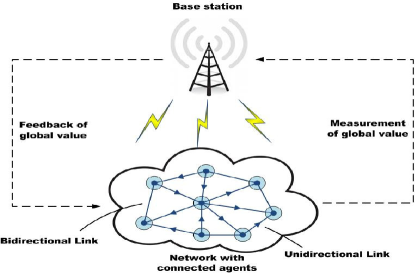
Figure 1: Schematic diagram of the optimisation framework

The specific mathematical problem we wish to solve is to find an optimal consensus point satisfying $x^{*}=y^{*}e$ such that the following optimisation problem is solved:

$$\underset{x\in\mathbb{R}^{\textrm{N}}}{\text{minimise}}\quad\sum\limits_{i=1}^{N}f_{i}(x_{i})\quad\text{subject to }x_{i}=x_{j},\,\,\,i,j\in\textrm{\text@underline{N}}\,.$$ (33)

After finding this common suggested speed, drivers are encouraged to drive at this recommended speed to minimise group emissions. Note in this study we use COPERT emission functions [2], but it is also possible to measure these average-speed functions in the car so as to incorporate individual driver behaviour.

In what follows, we wish to use an iterative feedback scheme of the form (21) to solve the optimisation problem (33). We will require that this problem has a unique solution and derive the specific form for $G$ in (21) from first order optimality conditions. To this end, it follows from elementary optimisation theory that when the $f_{i}$’s are strictly convex, the optimisation problem will be solved if and only if there exists a unique $y^{*}\in\mathbb{R}$ such that $\sum_{i=1}^{N}f^{\prime}_{i}(y^{*})=0.$ With this in mind we apply a feedback signal $G(x)=-\mu\sum_{i=1}^{N}f^{\prime}_{i}(x_{i})$ where $\mu\in\mathbb{R}$ is a parameter to be determined. This gives rise to the following dynamical system

$$x(k+1)=P(k)x(k)-\mu\sum_{i=1}^{N}f^{\prime}_{i}(x_{i}(k))e$$ (34)

where for each $k$ we define $P(k)$ as

$$P_{{i}{j}}\left(k\right)=\left\{\begin{array}[]{cl}\displaystyle{1-\sum_{{j}\in N_{k}^{{i}}}\eta_{{j}}}&\mbox{if }{j}={i}\\ \eta_{{j}}&\mbox{if }{j}\in N_{k}^{{i}}\\ 0&\mbox{otherwise}\end{array}\right.$$ (35)

where $\eta_{{j}}\in\mathbb{R}$ is a weighting factor, and $N_{k}^{{i}}$ represents the set of neighbour agents communicating to the $i^{\textrm{th}}$ vehicle.

As we assume that the $f_{i}$ are strictly convex, their derivatives are strictly increasing. We assume that each $f^{\prime}_{i}$ has a strictly positive and bounded growth, i.e., there exist constants $d_{\min}^{(i)}$ and $d_{\max}^{(i)}$; such that for any $a\neq b$

$$0<d_{\min}^{(i)}\leq\frac{f^{\prime}_{i}(a)-f^{\prime}_{i}(b)}{a-b}\leq d_{\max}^{(i)}\qquad\forall i\in\textrm{\text@underline{N}}.$$ (36)

We claim that provided $\mu$ is chosen according to

$0<\mu<2\left(\sum\limits_{i=1}^{N}d_{\max}^{(i)}\right)^{-1}$ then (34) is uniformly globally asymptotically stable at the unique optimal point $x^{*}e$ of the optimisation problem (33). First, we consider the scalar system associated with (34) which is given by

$$y(k+1)=y(k)-\mu\sum_{i=1}^{N}f^{\prime}_{i}(y(k)).$$ (37)

Note first that the fixed point condition for (37) is $\sum_{i=1}^{N}f^{\prime}_{i}(y^{*})=0$. So that a fixed point $y^{*}$ of (37), gives rise, by Lemma 1 to a fixed point of (34), which satisfies the necessary and sufficient conditions for optimality. Now, we wish to use Theorem 7 to show global asymptotic stability. To this end, we need to verify that system (34) satisfies all the conditions required in Theorem 7. The condition on $\mu$ ensures that the right hand side of (37) is in fact a strict contraction on $\mathbb{R}$. It follows from our comments after Lemma 5 that the assumption (ii) of Lemma 5 is satisfied. To show the Lipschitz condition (i) note that by (36) each $f^{\prime}_{i}$ is globally Lipschitz. As the coordinate functions are globally Lipschitz and sums of globally Lipschitz functions retain that property we obtain condition (ii).

To illustrate this application we consider 20 vehicles travelling along a section of road with random initial suggested speeds uniformly distributed between 60km/h and 70km/h. We assumed that there were 10 vehicles for each emission class, and the parameters set of the cost function for each class was chosen as R007 and R104, respectively, from [10]. The simulation results are presented in Fig. 2. Our results show that the recommended speeds of vehicles will asymptotically converge to the optimal one in less than 100 algorithm iterations.

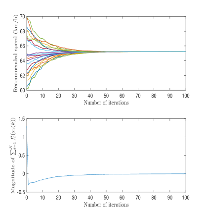
Figure 2: Dynamics of the state variables $x(k)$ with $\mu=0.1$

Remark 10.

Our main results are directed at consensus type applications where a basic type of ergodicity is assumed to hold. Clearly, this assumption is not always true. However, we note the following facts which are pertinent for applications in intelligent transportation systems (ITS), each of which make the assumption of strong ergodicity plausible.

• We are primarily motivated by ITS applications in which agents (cars) are travelling in close proximity to each other, thereby giving rise to connected communication graphs [10]. In areas of sparsely connected cars, roadside infrastructure can play a role in controlling the connectivity of the graph.
  

• Many applications of this type also operate a form of topology control to ensure either spatial or temporal connectivity. Details of one such algorithm is given in [6, 7].
  

• Any real SAS system will almost certainly be augmented by a local vehicle-based vision system. This vision system can provide estimates of neighbouring vehicle speeds, and these can be used as a proxy for suggested speeds. Also, if drivers do not follow the suggested speed, and others do, then vehicles will become closer in space to each other, thereby making the graph more connected, and this will have the effect of making the graph strongly ergodic.
  

• Finally, the central authority can be used to send global information (other than derivatives), every so often, so as to make strong ergodicity even more likely.

5 Conclusion

In this note we present a rigorous proof of stability and convergence of a recently proposed consensus system with feedback. Examples are given to illustrate the usefulness of the algorithm. For other smart grid applications see [9].

This work was in part supported by Science Foundation Ireland under grant 11/PI/1177.

Mingming Liu received his B.E. and Ph.D. degrees from National University of Ireland Maynooth in 2011 and 2015 respectively. He is currently a Post-Doctoral Research Fellow with University College Dublin. His research interests are nonlinear system dynamics, distributed control and optimisation techniques with applications to smart grid and transportation systems.

Fabian Wirth received his PhD from the Institute of Dynamical Systems at the University of Bremen in 1995. He has since held positions in Bremen, at the Centre Automatique et Systèmes of Ecole des Mines, the Hamilton Institute at NUI Maynooth, Ireland, the University of Würzburg and IBM Research Ireland. He holds the chair at the University of Passau, Germany. His current interests include stability theory, queueing networks, switched systems and large scale networks with applications to networked systems and in the domain of smart cities.

Martin Corless is a Professor in the School of Aeronautics & Astronautics at Purdue University. He is also Visiting Professor at University College Dublin and an Adjunct Honorary Professor at The National University of Ireland, Maynooth. He received a B.E. from University College Dublin and a Ph.D. from the University of California at Berkeley; both degrees are in mechanical engineering. His research is concerned with obtaining tools which are useful in the robust analysis and control of systems containing significant uncertainty and in applying these results to aerospace and mechanical systems and to sensor and communication networks.

Robert Shorten is currently Professor of Control Engineering and Decision Science at University College Dublin. Prof. Shorten’s research spans a number of areas. He has been active in computer networking, automotive research, collaborative mobility (including smart transportation and electric vehicles), as well as basic control theory and linear algebra. His main field of theoretical research has been the study of hybrid dynamical systems.

References

- [1] V. Blondel, J. M. Hendrickx, A. Olshevsky, and J. Tsitsiklis. Convergence in multiagent coordination, consensus, and flocking. In Proc. IEEE Conference on Decision and Control, volume 44, pages 2996–3000, 2005.
- [2] P.G. Boulter, T.J. Barlow, and I.S. McCrae. Emission factors 2009: Report 3-exhaust emission factors for road vehicles in the United Kingdom. TRL Report PPR356. TRL Limited, Wokingham, 2009.
- [3] Mathias Burger, Giuseppe Notarstefano, and Frank Allgower. A polyhedral approximation framework for convex and robust distributed optimization. IEEE Transactions on Automatic Control, 59(2):384–395, 2014.
- [4] S. Chatterjee and E. Seneta. Towards consensus: some convergence theorems on repeated averaging. Journal of Applied Probability, 14(1):89–97, 1977.
- [5] Ilse C.F. Ipsen and Teresa M.0 Selee. Ergodicity coefficients defined by vector norms. SIAM Journal on Matrix Analysis and Applications, 32(1):153–200, 2011.
- [6] F. Knorn, R. Stanojevic, M. Corless, and R. Shorten. A framework for decentralised feedback connectivity control with application to sensor network. International Journal of Control, 82(11):2095–2114, 2009.
- [7] Florian Knorn, Martin Corless, and Robert Shorten. Results in cooperative control and implicit consensus. International Journal of Control, 84(3):476–495, 2011.
- [8] T.C. Lee and Z.-P. Jiang. On uniform global asymptotic stability of nonlinear discrete-time systems with applications. IEEE Transactions on Automatic Control, 51(10):1644–1660, 2006.
- [9] M. Liu, E. Crisostomi, Y. Gu, and R. Shorten. Optimal distributed consensus algorithm for fair V2G power dispatch in a microgrid. in Proceedings of the International Electric Vehicle Conference (IEVC), 2014.
- [10] M. Liu, R. H. Ordóñez-Hurtado, F. Wirth, Y. Gu, E. Crisostomi, and R. Shorten. A distributed and privacy-aware speed advisory system for optimizing conventional and electric vehicle networks. IEEE Transactions on Intelligent Transportation Systems, 17(5):1308–1318, 2016.
- [11] A. Lorıa and D. Nešic. Stability of time-varying discrete-time cascades. In Proc. 15th. IFAC World Congress, 2002.
- [12] A. Lorıa and D. Nešić. On uniform boundedness of parameterized discrete-time systems with decaying inputs: Applications to cascades. Systems & Control Letters, 49(3):163–174, 2003.
- [13] W. Lu, F.M. Atay, and J. Jost. Synchronization of discrete-time dynamical networks with time-varying couplings. SIAM Journal on Mathematical Analysis, 39(4):1231–1259, 2007.
- [14] M. Mesbahi and M. Egerstedt. Graph Theoretic Methods in Multiagent Networks. Princeton University Press, 2010.
- [15] L. Moreau. Stability of multiagent systems with time-dependent communication links. IEEE Transactions on Automatic Control, 50(2):169–182, 2005.
- [16] A. Nedic, A. Ozdaglar, and P. A. Parrilo. Constrained consensus and optimization in multi-agent networks. IEEE Transactions on Automatic Control, 55(4):922–938, 2010.
- [17] D. Nešić and A. Loría. On uniform asymptotic stability of time-varying parameterized discrete-time cascades. IEEE Transactions on Automatic Control, 49(6):875–887, 2004.
- [18] R. Olfati-Saber, J. A. Fax, and R. M. Murray. Consensus and cooperation in networked multi-agent systems. Proceedings of the IEEE, 95(1):215–233, 2007.
- [19] A. Schlote, F. Häusler, T. Hecker, A. Bergmann, E. Crisostomi, I. Radusch, and R. Shorten. Cooperative regulation and trading of emissions using plug-in hybrid vehicles. IEEE Transactions on Intelligent Transportation Systems, 14(4):1572–1585, 2013.
- [20] G. Shi, K. H. Johansson, and Y. Hong. Reaching an optimal consensus: dynamical systems that compute intersections of convex sets. IEEE Transactions on Automatic Control, 58(3):610–622, 2013.