Branching Brownian motion with absorption and the all-time minimum of branching Brownian motion with drift

Abstract

We study a dyadic branching Brownian motion on the real line with absorption at 0, drift $\mu\in\mathbb{R}$ and started from a single particle at position $x>0.$ When $\mu$ is large enough so that the process has a positive probability of survival, we consider ${K}(t),$ the number of individuals absorbed at 0 by time $t$ and for $s\geq 0$ the functions ${\omega}_{s}(x):=\mathbb{E}^{x}[s^{{K}(\infty)}].$ We show that ${\omega}_{s}<\infty$ if and only of $s\in[0,s_{0}]$ for some $s_{0}>1$ and we study the properties of these functions. Furthermore, for $s=0,{\omega}(x):={\omega}_{0}(x)=\mathbb{P}^{x}({K}(\infty)=0)$ is the cumulative distribution function of the all time minimum of the branching Brownian motion with drift started at 0 without absorption.

We give three descriptions of the family ${\omega}_{s},s\in[0,s_{0}]$ through a single pair of functions, as the two extremal solutions of the Kolmogorov-Petrovskii-Piskunov (KPP) traveling wave equation on the half-line, through a martingale representation and as an explicit series expansion. We also obtain a precise result concerning the tail behavior of ${K}(\infty)$. In addition, in the regime where ${K}(\infty)>0$ almost surely, we show that $u(x,t):=\mathbb{P}^{x}({K}(t)=0)$ suitably centered converges to the KPP critical travelling wave on the whole real line.

1 Introduction

Consider a branching Brownian motion in which particles move according to a Brownian motion with drift $\mu\in\mathbb{R}$ and split into two particles at rate $\beta$ independently one from another. Call ${\mathcal{N}_{\text{all}}}(t)$ the population of all particles at time $t$ and call $X_{u}(t)$ the position of a given particle $u\in{\mathcal{N}_{\text{all}}}(t)$. When we start with a single particle at position $x$ we write $\mathbb{P}^{x}$ for the law of this process.

In a seminal paper, [13], Kesten considered the branching Brownian motion with absorption, i.e. the model just described with the additional property that particles entering the negative half-line $(-\infty,0]$ are immediately absorbed and removed. We write $\mathcal{N}_{\text{live}}(t)$ for the set of particles alive (not absorbed) in the branching Brownian motion with absorption and ${K}(t)$ the number of particles that have been absorbed up to time $t$. The system with absorption is said to become extinct if $\exists t\geq 0:\mathcal{N}_{\text{live}}(t)=\emptyset$ and to survive otherwise. We let ${K}(\infty):=\lim_{t\to\infty}{K}(t)\in\mathbb{R}\cup\{\infty\}$.

Depending on the value of $\mu$ one has the following behaviours (see Figure 1)

• if $\mu\leq-\sqrt{2\beta}$, the drift towards origin is so large that the system goes extinct almost surely. ${K}(\infty)$ is finite and non-zero.

• if $-\sqrt{2\beta}<\mu<\sqrt{2\beta}$ there is a non-zero probability of survival. On survival, there will always be particles near 0 and ${K}(\infty)=\infty$ almost surely.

• if $\mu\geq\sqrt{2\beta}$ there is still a non-zero probability of survival, but the system is drifting so fast away from 0 that, on survival, $\min_{u\in{\mathcal{N}_{\text{all}}}(t)}X_{u}(t)$ drifts to $+\infty$ almost surely as $t\to\infty$; ${K}(\infty)$ is thus almost surely finite. Furthermore, there is a non-zero probability that ${K}(\infty)=0$.

Figure 1: The three regimes: The hashed region represents the cone in which one expects to find particles.

The behaviour of ${K}(\infty)$ in regime $A$ ($\mu\leq-\sqrt{2\beta}$) has been the subject of very active research recently, including a conjecture by Aldous which was recently settled by P. Maillard [15] (we discuss Maillard’s results bellow), improving earlier results of L. Addario-Berry and N. Broutin [1] and E. Aïdékon [2]. Surprisingly, relatively little was known concerning the regimes B and C. Our main results in the present work concern the study of ${K}(\infty)$ and of certain related KPP-type equations.

1.1 The tail behaviour of ${K}(\infty)$

In [15], Pascal Maillard has shown that in regime A ($\mu\leq-\sqrt{2\beta}$) the variable ${K}(\infty)$ has a very fat tail. More precisely he shows that, as $z\to\infty$, there exists two constants $c,c^{\prime}$ which depend on $x$ such that

$$\mathbb{P}^{x}[{K}(\infty)>z]\sim\begin{cases}c/(z\log(z)^{2})&\text{for $\mu=-\sqrt{2\beta}$},\\[2.15277pt] c^{\prime}z^{-a(\mu)}&\text{for $\mu<-\sqrt{2\beta}$ where $a(\mu)=\frac{\mu+\sqrt{\mu^{2}-2\beta}}{\mu-\sqrt{\mu^{2}-2\beta}}$.}\end{cases}$$

In regime B ($-\sqrt{2\beta}<\mu<\sqrt{2\beta}$) it is clear that ${K}(\infty)=\infty$ on survival so one would essntially condition on extinction to study the tail behaviour of ${K}(\infty)$. This is outside the scope of the present work.

In regime C ($\mu\geq\sqrt{2\beta}$), however, ${K}(\infty)$ is almost surely finite. We introduce for $s\geq 0$ and $x\geq 0$,

$${\omega}_{s}(x):=\mathbb{E}^{x}\big{[}s^{{K}(\infty)}\big{]},\quad{\omega}_{s}(0)=s.$$ (1)

When $s\in[0,1]$ this quantity is the generating function of $K(\infty)$. We show that $\omega_{s}(x)$ is finite for some values of $s$ larger than 1:

Theorem 1.

In regime C ($\mu\geq\sqrt{2\beta}$), there exists a finite $s_{0}>1$ depending only on $\mu/\sqrt{\beta}$ such that

1. For $s\leq s_{0}$, ${\omega}_{s}(x)$ is finite for all $x\geq 0$,

2. For $s>s_{0}$, ${\omega}_{s}(x)$ is infinite for all $x>0$.

The functions $x\mapsto{\omega}_{s}(x)$ are increasing for any $s\in[0,1)$ and decreasing for any $s\in(1,s_{0}]$, converging to 1 when $x\to\infty$, and one has ${\omega}^{\prime}_{s_{0}}(0)=0$.

Furthermore, one has for $n$ large

$$\mathbb{P}^{x}[{K}(\infty)=n]\sim{-{\omega}_{s_{0}}^{\prime}(x)\over 2s_{0}^{n}n^{\frac{3}{2}}\sqrt{\pi\beta(s_{0}-1)}}.$$ (2)

Using the branching structure and a simple coupling allows to relate the ${\omega}_{s}(x)$ with each others, as in the following result (which is already present in [17, 15]):

Theorem 2.

In regime C ($\mu\geq\sqrt{2\beta}$),

1. For each $s\in[0,1)$,  ${\omega}_{s}(x)={\omega}_{0}(x+{\omega}_{0}^{-1}(s))$,

2. For each $s\in(1,s_{0}]$,  ${\omega}_{s}(x)={\omega}_{s_{0}}(x+{\omega}_{s_{0}}^{-1}(s)).$

We do not have an explicit expression for $s_{0}$ as a function of $\mu/\sqrt{\beta}$, but we can evaluate it numerically with a good precision as shown in Figure 2. In the critical case $\mu=\sqrt{2\beta}$, we obtain $s_{0}=1.3486\ldots$.

Figure 2: Numerical determination of $s_{0}$ and $s_{0}\beta/\mu^{2}$ as functions of $\mu/\sqrt{\beta}$.

We can prove the following property:

Proposition 3.

$s_{0}$ is an increasing function of $\mu/\sqrt{\beta}$ and furthermore $s_{0}\sim c\mu^{2}/\beta$ for some constant $c$ as $\mu/\sqrt{\beta}\to\infty$.

1.2 Distribution of the all-time minimum in a branching Brownian motion

The probability that $K(\infty)=0$ for a system started from $x$, is also the probability that the all-time minimum of a full branching Brownian motion with drift $\mu$ started from zero does not go below $-x$:

$${\omega}(x):={\omega}_{0}(x)=\mathbb{P}^{x}[{K}(\infty)=0]=\mathbb{P}^{0}[\min_{t\geq 0}\min_{u\in{\mathcal{N}_{\text{all}}}(t)}X_{u}(t)>-x].$$ (3)

This quantity, of course, is not trivial only in regime C ($\mu\geq\sqrt{2\beta}$). Then, since

$$\lim_{t\to\infty}\min_{u\in{\mathcal{N}_{\text{all}}}(t)}X_{u}(t)=+\infty$$

almost surely, we see that there is a well defined all-time minimum for the branching Bownian motion and we conclude that $\lim_{x\to\infty}{\omega}(x)=1.$

It is not hard to see by standard arguments that ${\omega}$ must satisfy a KPP-type differential equation with boundary conditions:

$$\begin{cases}0=\frac{1}{2}{\omega}^{\prime\prime}+\mu{\omega}^{\prime}+\beta({\omega}^{2}-{\omega}),&x\geq 0,\\ {\omega}(0)=0,\ \ {\omega}(\infty)=1.\end{cases}$$ (4)

In fact, ${\omega}_{s}(x)$ introduced in (1), if finte, is solution to the same equation with the boundary condition ${\omega}(0)=0$ replaced by ${\omega}_{s}(0)=s$:

$$\begin{cases}0=\frac{1}{2}{\omega}_{s}^{\prime\prime}+\mu{\omega}_{s}^{\prime}+\beta({\omega}_{s}^{2}-{\omega}_{s}),&x\geq 0,\\ {\omega}_{s}(0)=s,\ \ {\omega}_{s}(\infty)=1.\end{cases}$$ (5)

This is an example of the deep connection between branching Brownian motion and the KPP equation which goes back to McKean [16] who noticed that one can represent solutions of the KPP equation as expectations of functionals of branching Brownian motions.

Until now this is very classical, however there is one unexpected difficulty here: both (4) and (5) admit infinitely many solutions and are not sufficient to characterize ${\omega}(x)$. Figure 3 gives several numerical solutions to (4).

Figure 3: Solutions to (4) for $\beta=1$ and $\mu=2$. The red (bold) curve is ${\omega}$.

In this work , we present three largely independent ways to characterize ${\omega}(x)$ which are laid out in the three following subsections. The first approach relies on partial differential equations, the second gives ${\omega}(x)$ as the expectation of a certain martingale and the third one gives ${\omega}(x)$ as a power series.

One salient property of ${\omega}$ is that it converges to 1 rather quickly:

Proposition 4.

There exists $B>0$ such that

$$1-{\omega}(x)\sim Be^{-\big{(}\mu+\sqrt{\mu^{2}-2\beta}\big{)}x}\qquad\text{for large $x$}.$$ (6)

Furthermore, ${\omega}(x)$ is the only solution of (4) which remains in $[0,1)$ and converges that fast to 1.

Similarly, for any $s\in[0,s_{0})$, there exists $B_{s}\in\mathbb{R}$ such that

$$1-{\omega}_{s}(x)\sim B_{s}e^{-\big{(}\mu+\sqrt{\mu^{2}-2\beta}\big{)}x}\qquad\text{for large $x$}$$ (7)

where $B_{1}=0,$ $B_{s}>0$ when $s<1$ and $B_{s}<0$ when $s>1$.

This fast decay was actually an unexpected result for reasons explained in Section 1.2.4.

To simplify notation, we call $r$ the exponential decay rate of $1-{\omega}(x)$ as given in (6):

$$r:=\mu+\sqrt{\mu^{2}-2\beta}.$$ (8)

It is the largest solution of $\frac{1}{2}r^{2}-\mu r+\beta=0$.

1.2.1 ${\omega}(x)$ from partial differential equations

A first way to characterize ${\omega}(x)$ is to track the probability that no particle got absorbed up to time $t$. Define

$${u}(t,x):=\mathbb{P}^{x}[{K}(t)=0].$$ (9)

The function ${u}:\mathbb{R}_{+}^{2}\mapsto[0,1]$ is increasing in $x$ and decreasing in $t$ and, clearly, for each $x$, ${u}(t,x)\to{\omega}(x)$ as $t\to\infty$. Furthermore, ${u}$ satisfies the KPP equation with boundary conditions

$$\begin{cases}\partial_{t}{u}=\frac{1}{2}\partial_{xx}{u}+\mu\partial_{x}{u}+\beta({u}^{2}-{u}),\\ {u}(t,0)=0\ (\forall t\geq 0),\quad{u}(0,x)=1\ (\forall x>0),\end{cases}$$ (10)

which, by Cauchy’s Theorem has only one solution.

Therefore, to obtain ${\omega}(x)$, one can in principle solve (10) and take the large time limit. This route leads to the following Theorem:

Theorem 5.

In regime C ($\mu\geq\sqrt{2\beta}$), the function ${\omega}(x)$ defined by (3) is the maximal solution of (4) such that ${\omega}(x)<1$ for all $x\geq 0$.

More generally, $\omega_{s}(x)$ for $s<1$ is the maximal solution of (5) that stays below 1 and $\omega_{s}(x)$ for $s\in(1,s_{0}]$ is the minimal solution of (5) that stays above 1.

1.2.2 Martingale representation for ${\omega}$

There is an explicit probabilistic representation of the maximum standing wave ${\omega}$ in regime C ($\mu\geq\sqrt{2\beta}$). Recall that ${\mathcal{N}_{\text{all}}}(t)$ is the population of all the particles in the branching Brownian motion with no absorption and $\mathcal{N}_{\text{live}}(t)$ is the population of particles alive at time $t$ when we kill at 0. We now define on the same probability space a third process based on the branching Brownian motion in which particles that hit 0 are stopped but not removed from the system (they neither move nor branch). We denote by ${\mathcal{N}_{\text{live+abs.}}}(t)$ the set of particles alive at time $t$ in this model. With a slight abuse of notations we continue to write $X_{u}(t)$ for the positions of particles when $u\in{\mathcal{N}_{\text{live+abs.}}}(t).$

Let us define the following two processes:

$${Z}_{\mathrm{live+abs.}}(t):=\sum_{u\in{\mathcal{N}_{\text{live+abs.}}}(t)}e^{-rX_{u}(t)},\qquad{Z}_{\text{all}}(t):=\sum_{u\in{\mathcal{N}_{\text{all}}}(t)}e^{-rX_{u}(t)},$$ (11)

where $r$ is the asymptotic decay of ${\omega}(x)$ as given in (8). Rewriting $X_{u}(t)=Y_{u}(t)+\mu t$ it is clear that $\big{\{}Y_{u}(t),u\in{\mathcal{N}_{\text{all}}}(t)\big{\}}$ is simply a standard branching Brownian motion with no drift. Therefore ${Z}_{\text{all}}$ is the usual exponential martingale with parameter $r$ associated with the branching Brownian motion $Y.$ The process ${Z}_{\mathrm{live+abs.}}$ is the martingale ${Z}_{\text{all}}$ stopped on the line $t\wedge T_{0}$ (i.e. particles are stopped at time $t$ or when they hit 0 for the first time). It is therefore also a martingale.

Lemma 6.

In regime C ($\mu\geq\sqrt{2\beta}$) the martingale $({Z}_{\mathrm{live+abs.}}(t),t\geq 0)$ converges almost surely and in $L^{1}$ to ${K}(\infty)$ and therefore $\mathbb{E}^{x}[{K}(\infty)]={Z}_{\mathrm{live+abs.}}(0)=e^{-rx}.$

Following the probability tilting method pioneered by [14] and [8] we introduce a new probability measure $\mathbb{Q}^{x}$

$$\frac{\mathrm{d}\mathbb{Q}^{x}}{\mathrm{d}\mathbb{P}^{x}}=e^{rx}{K}(\infty).$$

Note that since ${Z}_{\mathrm{live+abs.}}$ is a closed martingale we have that $\mathbb{E}^{x}[{K}(\infty)|\mathcal{F}_{t}]={Z}_{\mathrm{live+abs.}}(t).$ Thus

$$\left.\frac{\mathrm{d}\mathbb{Q}^{x}}{\mathrm{d}\mathbb{P}^{x}}\right|_{\mathcal{F}_{t}}=\frac{{Z}_{\mathrm{live+abs.}}(t)}{{Z}_{\mathrm{live+abs.}}(0)}.$$

Under this tilted probability measure, the law of the process is the same as the original $\mathbb{P}^{x}$ law except for the movement and branching rate of a distinguished particle (the spine particle $\xi$). The spine moves according to a Brownian motion with drift $-\sqrt{\mu^{2}-2\beta}$, branches at an accelerated rate of $2\beta$ and stops (i.e. sticks and stops reproducing) upon hitting 0.

Theorem 7.

In regime C ($\mu\geq\sqrt{2\beta}$),

$$1-{\omega}(x)=\mathbb{Q}^{x}\bigg{(}\frac{1}{{K}(\infty)}\bigg{)}e^{-rx}.$$

Furthermore, $\mathbb{Q}^{x}\big{(}\frac{1}{{K}(\infty)}\big{)}$ converges to a finite constant $B>0$ when $x\to\infty$ and thus, as $x\to\infty$,

$$1-{\omega}(x)\sim Be^{-rx}.$$

More generally, for any $s\in[0,s_{0}]$, one has

$$1-{\omega}_{s}(x)=\mathbb{Q}^{x}\bigg{(}\frac{1-s^{{K}(\infty)}}{{K}(\infty)}\bigg{)}e^{-rx}$$

and the expectation $\mathbb{Q}^{x}(\cdot)$ converges to a finite positive constant as $x\to\infty$.

We will see in the proof that we can give an explicit representation of the constant $B$ which appears in Proposition 4 as the expectation of ${K}(\infty)^{-1}$ under the measure $\mathbb{Q}^{\infty}$ (similar to $\mathbb{Q}^{x}$ but with the spine particle “started at infinity”).

1.2.3 ${\omega}(x)$ as a series expansion

The function ${\omega}(x)$ can be understood in terms of series expansion. Let $\{a_{n}\}_{n\geq 1}$ be the sequence defined by

$$a_{1}=1,\qquad a_{n}=\frac{\beta}{\frac{1}{2}n^{2}r^{2}-n\mu r+\beta}\sum_{j=1}^{n-1}a_{j}a_{n-j}=\frac{1}{(n-1)\big{(}\frac{r^{2}}{2\beta}n-1\big{)}}\sum_{j=1}^{n-1}a_{j}a_{n-j},\quad n\geq 2,$$ (12)

(recall that $r$ was defined in (8), that $\frac{1}{2}r^{2}-\mu r+\beta=0$ and that $r\geq\mu\geq\sqrt{2\beta}$) and $\Phi$ the function defined by the series

$$\Phi(z)=\sum_{n\geq 1}a_{n}z^{n}.$$ (13)

We have

Proposition 8.

The radius of convergence $\mathcal{R}$ of $\Phi$ is non-zero and there exists $B\in(0,\mathcal{R})$ such that

$$\omega(x)=1-\Phi(Be^{-rx}).$$

More generally, for any $0\leq s\leq s_{0}$, there exists a number $B_{s}$ such that

$$\omega_{s}(x)=1-\Phi(B_{s}e^{-rx})\qquad\text{for all $x\geq 0$ such that $|B_{s}|e^{-rx}<\mathcal{R}$}.$$ (14)

$s\mapsto B_{s}$ is decreasing, positive for $s<1$, zero for $s=1$, and negative for $s>1$. In particular, for $s\leq 1$, the condition $|B_{s}|e^{-rx}<\mathcal{R}$ is automatically fulfilled.

The proof is contained in Section 2.2.4. Numerically, it seems that $\mathcal{R}$ is large enough that $|B_{s}|e^{-rx}<\mathcal{R}$ for all $s\in[0,s_{0}]$ and all $x\geq 0$, but we haven’t proved that point. The representation (14) makes it very easy to compute numerically ${\omega}_{s}$ by first computing $\Phi(z)$, see Figure 4; the value $s_{0}$ is then obtained as 1 minus the first minimum of $\Phi$ for negative arguments. This follows easily from the facts that $w^{\prime}_{s_{0}}=0,w^{\prime\prime}_{s_{0}}<0$ and that $w^{\prime}_{s}(0)<0$ for all $s\in(1,s_{0})$.

, 

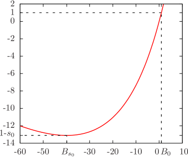
Figure 4: The function $z\mapsto\Phi(z)$ for $\beta=1$ and $\mu=\sqrt{2}$ (left) or $\mu=3$ (right). Numerically, one has $s_{0}\approx 1.35$, $B_{s_{0}}\approx-0.859$, $B_{0}\approx 0.564$, $\mathcal{R}\approx 3.14$ for $\mu=\sqrt{2}$ and $s_{0}\approx 14.11$, $B_{s_{0}}\approx-39.86$, $B_{0}\approx 0.969$, $\mathcal{R}\approx 72.8$ for $\mu=3$.

1.2.4 About the asymptotic decay (6)

The KPP partial differential equation,

$$\partial_{t}h=\frac{1}{2}\partial_{xx}h+\beta(h^{2}-h),$$ (15)

where $0\leq h(t,x)\leq 1$, $h(t,-\infty)=0$ and $h(t,+\infty)=1$, describes how a stable phase ($h=0$ on the left) invades an unstable phase ($h=1$ on the right). It is well known that it admits travelling wave solutions of the form

$$h(t,x)=h_{\mu}(x-\mu t),\qquad 0<h_{\mu}<1,\qquad h_{\mu}(+\infty)=1,\qquad h_{\mu}(-\infty)=0,$$

for any velocity $\mu$ greater or equal to $\sqrt{2\beta}$. The travelling wave $x\mapsto h_{\mu}(x)$ is then solution to

$$\frac{1}{2}h_{\mu}^{\prime\prime}+\mu h_{\mu}^{\prime}+\beta(h_{\mu}^{2}-h_{\mu})=0,\quad h_{\mu}(-\infty)=0,\quad h_{\mu}(+\infty)=1.$$ (16)

The solution to (16) is unique up to translation.

Equation (16) for $h_{\mu}$ is very similar to equation (4) for ${\omega}(x)$, but $h_{\mu}$, surprisingly, does not have the same asymptotic behaviour as ${\omega}$ for large $x$, in the region where $h_{\mu}$ and ${\omega}$ are close to 1. Indeed, linearising (16) around 1, one gets

$$\frac{1}{2}(1-\tilde{h}_{\mu})^{\prime\prime}+\mu(1-\tilde{h}_{\mu})^{\prime}+\beta(1-\tilde{h}_{\mu})=0,\quad\text{[linearized]}$$ (17)

(a term of order $(1-\tilde{h}_{\mu})^{2}$ has been neglected) and the general solution to (17) is, for some constants $A$ and $B$,

$$1-\tilde{h}_{\mu}(x)=\begin{cases}Ae^{-\big{(}\mu-\sqrt{\mu^{2}-2\beta}\big{)}x}+Be^{-\big{(}\mu+\sqrt{\mu^{2}-2\beta}\big{)}x}&\text{for $\mu>\sqrt{2\beta}$},\\ (Ax+B)e^{-\sqrt{2\beta}\,x}&\text{for $\mu=\sqrt{2\beta}$}.\\ \end{cases}\quad\text{[linearized]}$$ (18)

For $x$ large, $\tilde{h}_{\mu}$ is close to $h_{\mu}$ with the meaning that for some constant $A$ and $B$, $1-\tilde{h}_{\mu}\sim 1-h_{\mu}$ (see the discussion in Section 2.2.3). Of course, if $A\neq 0$, the term in factor of $B$ is negligible compared to the term in factor of $A$ and the $A$ term alone is an equivalent to $1-h_{\mu}$. When solving (16), it turns out that the solution has a non-zero $A$ term and that, therefore,

$$1-h_{\mu}(x)\sim\begin{cases}Ae^{-\big{(}\mu-\sqrt{\mu^{2}-2\beta}\big{)}x}&\text{for $\mu>\sqrt{2\beta}$},\\ Axe^{-\sqrt{2\beta x}}&\text{for $\mu=\sqrt{2\beta}$},\end{cases}$$ (19)

where $A$ depends on $\mu$.

We now consider equation (4) for ${\omega}(x)$. Of course, the boundary condition of (4) is not sufficient to determine a unique solution, and for a range of values of $c$ there exists a solution to

$$0=\frac{1}{2}v^{\prime\prime}+\mu v^{\prime}+\beta(v^{2}-v),\quad v(+\infty)=1,\quad v(0)=0,\quad v^{\prime}(0)=c.$$ (20)

(The difference with equation (4) for ${\omega}(x)$ is the added condition $v^{\prime}(0)=c$. Figure 3 shows several solutions.)

One can then do, as above, a large $x$ analysis of $v$ and, the partial differential equation being the same, one finds again that $1-v\sim 1-\tilde{h}_{\mu}$ ($x$ large) as given in (18) for some $c$ and $\mu$ dependent values of $A$ and $B$. Generically, $A$ is non-zero and $1-v$ decays as $1-h_{\mu}$ in (19) (up to a multiplicative constant; the $A$ is usually different and can even be negative, see Figure 3).

However, for a well chosen value of $c$ (depending on $\mu$), one has $A=0$, and the asymptotic decay of $1-v$ is given by the $B$ term (that is: it decays much faster). The meaning of Proposition 4 is that ${\omega}(x)$ is precisely that very special solution to (4) that decays unlike all the other ones and unlike the travelling wave $h_{\mu}$.

It is also interesting to remark that an equation very similar to (4) appears in the study [11, 6] of the the extinction probability of a branching Brownian motion with absorption and supercritical drift $\mu>-\sqrt{2\beta}$ (regimes B and C): let $\theta(x)=\mathbb{P}^{x}[\mathcal{N}_{\text{live}}(\infty)=\emptyset]$ be the extinction probability when the system is started from $x$; then one has

$$\begin{cases}0=\frac{1}{2}\theta^{\prime\prime}+\mu\theta^{\prime}+\beta(\theta^{2}-\theta),&x\geq 0,\\ \theta(0)=1,\ \theta(\infty)=0.\end{cases}$$ (21)

Equations (4) and (21) differ only by their boundary conditions; however (21) has a unique solution, whereas (4) has many.

A possible way to understand the difference is that an asymptotic analysis of $\theta(x)$ for large $x$ similar to (18) yields only one possible exponential decay: $\theta(x)\sim A\exp[-(\mu+\sqrt{\mu^{2}+2\beta})x]$ for some constant $A$, which means that, up to translations, there is only one solution which does converge to zero at infinity, whereas for ${\omega}(x)$ there were two possible exponential decays and infinitely many solutions. Otherwise said, if one were to impose $\theta(0)=1$ and $\theta^{\prime}(0)=-c$, there would only be one value of $c$ for which $\theta$ would converge to zero at infinity.

1.3 A travelling wave result

In regimes A and B ($\mu<\sqrt{2\beta}$) one has ${\omega}(x)=0$ because ${K}(\infty)>0$ almost surely, which is not very interesting. What is more interesting is the way that ${u}(t,x)$, defined in (9) as $\mathbb{P}^{x}\big{[}K(t)=0\big{]}$, converges to zero: it does so by assuming the shape of the critical travelling wave of the KPP equation. Let us recall quickly the well known facts on this critical travelling wave.

Consider the KPP equation (15) without drift on the whole line with Heaviside initial conditions:

$$\begin{cases}\partial_{t}h=\frac{1}{2}\partial_{xx}h+\beta(h^{2}-h),\\ h(0,x)=0\ (\forall x<0),\qquad h(0,x)=1\ (\forall x>0).\end{cases}$$ (22)

It is well known that $h(t,x)$ is the probability that the leftmost particle at time $t$ of a branching Brownian motion started at $x$ is to the right of zero. Furthermore, this probability converges to the critical travelling wave in the following sense:

$$h(t,m_{t}+x)\to h_{*}(x)\text{ uniformly in $x$ as $t\to\infty$}$$

with

$$m_{t}:=\sqrt{2\beta}\,t-\frac{3}{2\sqrt{2\beta}}\log t+\text{Cste}$$ (23)

and where $h_{*}:=h_{\sqrt{2\beta}}$ is the travelling wave moving at the minimal possible velocity $\sqrt{2\beta}$, see (16). To fix the invariance by translation, we impose the further condition $h_{*}(0)=1/2$:

$$\begin{cases}0=\frac{1}{2}h_{*}^{\prime\prime}+\sqrt{2\beta}\,h_{*}^{\prime}+\beta(h_{*}^{2}-h_{*}),\\ h_{*}(-\infty)=0,\quad h_{*}(0)=\frac{1}{2},\quad h_{*}(+\infty)=1,\end{cases}$$ (24)

and the solution to (24) is now unique.

Adding a drift $+\mu\partial_{x}h$ to (22) would only shift the solutions by $-\mu t$ and would make (22) very similar to (10): the only difference would be that ${u}$ is defined on $\mathbb{R}^{+}$ and $h$ on $\mathbb{R}$, but as both equations converge quickly to zero around the origin in regimes A and B $(\mu<\sqrt{2\beta})$, this difference turns out to be minimal and one has

Theorem 9.

In regimes A and B ($\mu<\sqrt{2\beta}$), there exists a constant $C$ depending on $\mu$ and $\beta$ such that

$${u}(t,x+m_{t}-\mu t+C)\to h_{*}(x)\quad\text{uniformly in }x\text{ as }t\to\infty$$

where $m_{t}$ is given by (23) and $h_{*}$ is the solution to (24).

It is interesting to compare this result about the behaviour of $u(t,x)=\mathbb{P}^{x}({K}(t)=0)$ when $\mu<\sqrt{2\beta}$ to the behaviour of the extinction probability ${\tilde{u}}(t,x)=\mathbb{P}^{x}(\mathcal{N}_{\text{live}}(t)=\emptyset)$ when $\mu\leq-\sqrt{2\beta}.$ It is not hard to see that ${\tilde{u}}$ satisfies the same equation (10) as $u$ with different boundary conditions, which is $1$ minus the boundary condition in (10); namely ${\tilde{u}}$ solves

$$\begin{cases}\partial_{t}{\tilde{u}}=\frac{1}{2}\partial_{xx}{\tilde{u}}+\mu\partial_{x}{\tilde{u}}+\beta({\tilde{u}}^{2}-{\tilde{u}}),\\ {\tilde{u}}(t,0)=1\ (\forall t\geq 0),\quad{u}(0,x)=0\ (\forall x>0),\end{cases}$$ (25)

What is particularly striking is that in the critical case $\mu=-\sqrt{2\beta}$ it is known since Kesten [13] (see also [5]) that to survive up to time $t$ one must start with an initial particle at position $x=ct^{1/3}$. This means that if ${\tilde{u}}(t,x+\tilde{m}_{t})$ converges to some limit front shape then the centering term giving the position of the front $\tilde{m}_{t}$ has to be of order $ct^{1/3}$. However the convergence of the solution of (25) to a travelling wave is at present an open problem.

2 Proofs

The proofs section are presented mostly in the same order as the results: Section 2.1 contains the proofs to Theorems 1 and 2 about the structure of the functions ${\omega}_{s}(x)=\mathbb{E}^{x}[s^{{K}(\infty)}]$ in regime C ($\mu\geq\sqrt{2\beta}$). Section 2.2 contains the proofs to Proposition 4, Theorem 5, Lemma 6, Theorem 7 and Proposition 8 about the different representations of ${\omega}(x)={\omega}_{0}(x)=\mathbb{P}^{x}[{K}(\infty)=0]$ in regime C ($\mu\geq\sqrt{2\beta}$). Finally, Section 2.3 contains the proof of Theorem 9 about the establishment of a travelling for ${u}(t,x)=\mathbb{P}^{x}[{K}(t)=0]$ in regimes A and B ($\mu<\sqrt{2\beta}$) and the asymptotic behavior of $s_{0}$ established in Proposition 3 is proven last.

2.1 Proof concerning the tail behaviour of ${K}(\infty)$

In this section we consider exclusively regime C ($\mu\geq\sqrt{2\beta}$) and we focus on the problem of the exponential moments of ${K}(\infty)$. We first establish some properties of ${\omega}_{s}(x)=\mathbb{E}^{x}[s^{{K}(\infty)}]$ as defined in (1) and proceed to prove Theorems 2 and Proposition 3. We then prove the asymptotic behaviour (LABEL:asymptNhits) to complete the proof of Theorem 1.

The first property we need is that for a given $s$, the quantity ${\omega}_{s}(x)$ is either finite for all $x>0$ or infinite for all $x>0$:

Lemma 10.

For a given $s$,

$$\big{(}\exists x>0\ :\ {\omega}_{s}(x)<+\infty\big{)}\Leftrightarrow\big{(}\forall x>0\ :\ {\omega}_{s}(x)<+\infty\big{)}.$$

Proof.

Fix $s>0$, $x>0$ and $y>0$. There is a positive probability, which we note $\epsilon(x,y)$, that the initial particle starting from $x$ reaches position $y$ before any branching or killing happens. Then

$${\omega}_{s}(x)=\mathbb{E}^{x}[s^{{K}(\infty)}]\geq\epsilon(x,y)\mathbb{E}^{y}[s^{{K}(\infty)}]=\epsilon(x,y){\omega}_{s}(y).$$

Therefore, if ${\omega}_{s}(x)$ is finite, then ${\omega}_{s}(y)$ is also finite. ∎

Remark: in the following, we write ${\omega}_{s}<\infty$ when the conditions of the lemma are met. Clearly, this is the case when $s\leq 1$. Furthermore, as $s\mapsto{\omega}_{s}(x)$ is obviously increasing, if ${\omega}_{s_{0}}<\infty$ for some $s_{0}$, then ${\omega}_{s}<\infty$ for all $s<s_{0}$.

When ${\omega}_{s}<\infty$, it is clear by standard arguments that ${\omega}_{s}(x)$ is solution to

$$\begin{cases}0=\frac{1}{2}{\omega}_{s}^{\prime\prime}+\mu{\omega}_{s}^{\prime}+\beta({\omega}_{s}^{2}-{\omega}_{s}),\\ {\omega}_{s}(0)=s.\end{cases}$$ (26)

Let us now prove Theorem 2. A slightly more general result is given by the following Lemma:

Lemma 11.

If ${\omega}_{s}<\infty$ then, for any $x\geq 0$ and $h\geq 0$,

$${\omega}_{s}(x+h)={\omega}_{{\omega}_{s}(h)}(x).$$

Setting $s=0$ and renaming ${\omega}_{0}(h)$ as $s$ gives the first line of the Theorem. Once we have proved that $s_{0}$ exists, setting $s=s_{0}$ and renaming ${\omega}_{s_{0}}(h)$ as $s$ gives the second line of the Theorem.

Proof.

Instead of starting our branching process at position $x$ and killing particles at $0$, it is here more convenient to think of the process as started at 0 and particles being absorbed at $-x$. This allows to couple different values of the killing position. In particular, if $\mathcal{H}_{x}$ designates the particles stopped when they first hit $-x$ and ${K}_{x}(\infty)$ is the number of particles in $\mathcal{H}_{x}$, we have that

$${\omega}_{s}(x+h)=\mathbb{E}\big{[}\prod_{u\in\mathcal{H}_{x}}s^{{K}^{(u)}_{h}(\infty)}\big{]}=\mathbb{E}\big{[}\prod_{u\in\mathcal{H}_{x}}{\omega}_{s}(h)\big{]}=\mathbb{E}\big{[}{\omega}_{s}(h)^{{K}_{x}(\infty)}\big{]}={\omega}_{{\omega}_{s}(h)}(x),$$

where ${K}^{(u)}_{h}(\infty)$ is the total number of descendent of the particle $u$ which are killed at $-x-h$ (which by translation invariance of the branching Brownian motion and the branching property is an independent copy of ${K}_{h}(\infty)$). ∎

We now have a monotonicity result:

Lemma 12.

1. If $s<1$, $x\mapsto{\omega}_{s}(x)$ is an increasing function converging to 1.

2. If $s>1$ and ${\omega}_{s}<\infty$, $x\mapsto{\omega}_{s}(x)$ is a decreasing function converging to 1.

Proof.

Once the increasing/decreasing part is proved, the fact that the limit is 1 is obvious: from its definition, it is clear that ${\omega}_{s}<1$ if $s<1$ and ${\omega}_{s}>1$ if $s>1$. Assuming ${\omega}_{s}$ is increasing or decreasing (depending on $s$), it must have a limit, and from (26) that limit must be 1.

From its interpretation as the distribution of the all-time minimum of a branching Brownian motion, see (3), it is furthermore clear that ${\omega}_{0}={\omega}$ is an increasing function. Then, the coupling provided by Lemma 11 (or more simply Theorem 2) implies that ${\omega}_{s}$ is an increasing function for all $s<1$.

Therefore, it only remains to prove that for $s>1$, ${\omega}_{s}$ is decreasing when it is finite.

Assume $s>1$ and ${\omega}_{s}<\infty$. We first show that ${\omega}_{s}$ is monotonous by considering two cases:

• If ${\omega}_{s}^{\prime}(0)>0$ then, for all $h>0$ small enough, ${\omega}_{s}(h)>s$. But, for $x$ fixed, $s\mapsto{\omega}_{s}(x)$ is a strictly increasing function so ${\omega}_{{\omega}_{s}(h)}(x)>{\omega}_{s}(x)$. Then by Lemma 11, ${\omega}_{s}(x+h)>{\omega}_{s}(x)$ for all $x$ and all $h>0$ small enough: ${\omega}_{s}$ is increasing.

• If ${\omega}_{s}^{\prime}(0)\leq 0$ then, for all $h>0$ small enough, ${\omega}_{s}(h)<s$ because in the limit case ${\omega}_{s}^{\prime}(0)=0$, one has ${\omega}_{s}^{\prime\prime}(0)<0$ from (26). Then, as in previous case, ${\omega}_{s}(x+h)={\omega}_{{\omega}_{s}(h)}(x)<{\omega}_{s}(x)$ for all $x$ and all $h>0$ small enough: ${\omega}_{s}$ is decreasing.

It now remains to rule out the possibility that ${\omega}_{s}$ is increasing for $s>1$. Imagine that $s>1$ and ${\omega}_{s}$ increases. Then, from (26), ${\omega}_{s}^{\prime\prime}(x)\leq-2\beta(\omega_{s}^{2}(x)-\omega_{s}(x))\leq-2\beta(s^{2}-s)$ and ${\omega}_{s}^{\prime}(x)\leq{\omega}_{s}^{\prime}(0)-2\beta(s^{2}-s)x$, which becomes negative for $x$ large enough, in contradiction with the fact that ${\omega}_{s}$ increases. So ${\omega}_{s}$ must decrease for $s>1$. ∎

We need now to characterize the values of $s$ for which ${\omega}_{s}<\infty$.

Lemma 13.

Assume $s>1$. If there exists a function $v$ which solves

$$\begin{cases}0=\frac{1}{2}v^{\prime\prime}+\mu v^{\prime}+\beta(v^{2}-v),\\ v(0)=s,\qquad v(x)\geq 1\ (\forall x\geq 0),\end{cases}$$ (27)

then ${\omega}_{s}<\infty$.

Remark: The converse is obvious: when ${\omega}_{s}$ is finite, it is one of the solutions to (27). This Lemma allows to define

$$s_{0} =\sup\big{\{}s\geq 1:{\omega}_{s}<\infty\big{\}},$$ (28)

$$=\sup\big{\{}s\geq 1:\text{a solution to \eqref{eqv} exists}\},$$

and because $s\mapsto{\omega}_{s}(x)$ increases, one has ${\omega}_{s}<\infty$ for all $s<s_{0}$.

Proof.

We present two proofs: one probabilistic and one analytical.

Choose $s>1$ such that (27) has a solution $v$. We introduce the process

$$M_{t}:=\prod_{u\in{\mathcal{N}_{\text{live+abs.}}}(t)}v\big{(}X_{u}(t)\big{)},$$

where we recall that ${\mathcal{N}_{\text{live+abs.}}}(t)$ is the set of particles in the branching Brownian motion where particles are frozen at the origin, see Section 1.2.2.

$M_{t}$ is a positive local martingale and therefore a positive super-martingale which thus converges almost surely to $M_{\infty}$. Observe that under $\mathbb{P}^{x}$

$$v(x)=M_{0}\geq\mathbb{E}^{x}(M_{t})\geq\mathbb{E}^{x}(M_{\infty}).$$

But since for all $t\geq 0$ one has

$$M_{t}\geq v(0)^{{K}(t)}=s^{{K}(t)},$$

we see that $M_{\infty}\geq s^{{K}(\infty)}$ and therefore

$${\omega}_{s}(x)=\mathbb{E}^{x}\big{[}s^{{K}(\infty)}\big{]}\leq v(x)<\infty.$$

The same result can be proved analytically through the maximum principle. Let us introduce

$${u}_{s}(t,x):=\mathbb{E}^{x}[s^{{K}(t)}],$$ (29)

which is clearly solution to

$$\begin{cases}\partial_{t}{u}_{s}=\frac{1}{2}\partial_{xx}{u}_{s}+\mu\partial_{x}{u}_{s}+\beta({u}_{s}^{2}-{u}_{s}),\qquad x\geq 0,\\ {u}_{s}(t,0)=s\ (\forall t\geq 0),\qquad{u}_{s}(0,x)=1\ (\forall x>0).\end{cases}$$ (30)

(Compare to (9).) With $v$ as above, one clearly has $\forall x\geq 0$, ${u}_{s}(0,x)\leq v(x)$. Therefore, by the maximum principle we have that

$${u}_{s}(t,x)\leq v(x),\qquad\forall t\geq 0,x\geq 0$$

and as ${u}_{s}(t,x)\nearrow{\omega}_{s}(x)$ as $t\to\infty$ we see that ${\omega}_{s}(x)\leq v(x)<\infty$. ∎

It is obvious that $s_{0}$ defined in (28) depends only on the ratio $\mu/\sqrt{\beta}$ by a simple scaling argument: the branching Brownian motion with drift $\mu$ and branching rate $\beta$ is transformed, when time is scaled by $\lambda$ and space by $\sqrt{\lambda}$, into a branching Brownian motion with drift $\mu\sqrt{\lambda}$ and branching rate $\beta\lambda$. In particular, ${\omega}_{s,\beta,\mu}(x)={\omega}_{s,\beta\lambda,\mu\sqrt{\lambda}}(\sqrt{\lambda}\,x)={\omega}_{s,1,\mu/\sqrt{\beta}}(x/\sqrt{\beta})$ with the obvious new notation. What remains to be shown are the following properties of ${\omega}_{s}$: $s_{0}$ is finite, ${\omega}_{s_{0}}$ is finite, ${\omega}_{s_{0}}^{\prime}(0)=0$ and $s_{0}>1$.

Lemma 14.

$s_{0}<\infty$, that is: ${K}(\infty)$ does not have exponential moments of all orders.

Proof.

For the system started from $x>0$, consider the following family of events for $n\in\mathbb{N}$:

$$\mathcal{A}_{n}=\begin{cases}{K}(\infty)=n,\quad\text{and}\\ \text{for all integers $i\leq n$, }{K}(i)=i,\quad\text{and}\\ \text{for all integers $i\leq n$, there is at time~{}$i$ only one particle alive and it sits in $[x,x+1]$.}\end{cases}$$

In words, for each $i\in\{0,1,\ldots,n-1\}$ there is one particle alive at time $i$, it sits in $[x,x+1]$, and during a time interval one, this particle splits exactly once, one the offspring gets absorbed and the other is again in $[x,x+1]$ at time $i+1$. The one particle alive at time $n$ generates a tree drifting to infinity with no more absorbed particles.

Let $\epsilon_{y,z}\mathrm{d}z$ be the probability that a particle sitting at $y$ has, during a time interval one, exactly one splitting event with one offspring being absorbed and the other one ending up in $\mathrm{d}z$. Define furthermore

$$q=\min_{y\in[x,x+1]}\int_{x}^{x+1}\epsilon_{y,z}\mathrm{d}z.$$

$q$ is the minimal probability for a particle sitting somewhere in $[x,x+1]$ to have, during a time interval one, exactly one splitting event with one offspring being absorbed and the other one ending up in $[x,x+1]$. It is clear that $q>0$ and that, furthermore,

$$\mathbb{P}^{x}({K}(\infty)=n)>\mathbb{P}^{x}(\mathcal{A}_{n})>q^{n}\mathbb{P}^{x}({K}(\infty)=0).$$

This implies that $\mathbb{E}^{x}[q^{-{K}(\infty)}]=\infty$ and that $s_{0}\leq 1/q<\infty$. ∎

Lemma 15.

${\omega}_{s_{0}}<\infty$.

Proof.

If $s_{0}=1$, this is trivial as ${\omega}_{1}=1$. Assume now $s_{0}>1$ and let us fix $x>0$. For any $1<s<s_{0}$, as ${\omega}_{s}$ is decreasing, one has ${\omega}_{s}(x)<s<s_{0}$. This implies that (using the monotone convergence Theorem) ${\omega}_{s_{0}}(x)=\lim_{s\nearrow s_{0}}{\omega}_{s}(x)$ is finite which entails the result. ∎

Lemma 16.

${\omega}_{s_{0}}^{\prime}(0)=0$.

Proof.

We already know that ${\omega}_{s_{0}}^{\prime}(0)\leq 0$. Assuming ${\omega}_{s_{0}}^{\prime}(0)<0$, one could continue the function ${\omega}_{s_{0}}$ to negative arguments using (27) and one could find a $x_{0}<0$ such that ${\omega}_{s_{0}}(x_{0})>s_{0}$; then the function $x\mapsto{\omega}_{s_{0}}(x_{0}+x)$ satisfies (27) with $s>s_{0}$, which is a contradiction. ∎

The proof that $s_{0}>1$ for all $\mu\geq\sqrt{2\beta}$ is divided into two steps. First, we show that $s_{0}>1$ in the critical case $\mu=\sqrt{2\beta}$. Then we conclude by proving Proposition 3, which states that $s_{0}$ is an increasing function of $\mu/\sqrt{\beta}$.

Lemma 17.

In the critical case $\mu=\sqrt{2\beta}$, for $s>1$ small enough, there exists solutions to (27), that is $s_{0}>1$.

Proof.

Assume $\mu=\sqrt{2\beta}$. After the change of variables $\ell(x):=e^{\mu x}\big{(}v(x)-1\big{)}$, (27) reads

$$\frac{1}{2}\ell^{\prime\prime}+\beta e^{-\mu x}\ell^{2}=0.$$ (31)

Let us consider the solution to (31) with $\ell(0)=\ell^{\prime}(0)=\epsilon$ for some $\epsilon>0$. We want to prove that $\forall x,\ell(x)>0$ if $\epsilon$ is small enough. Assume otherwise and call $x_{0}=\inf\{x\geq 0:\ell(x)=0\}$. Then, as $\ell^{\prime\prime}(x)\leq 0$, we have $\ell(x)\leq\epsilon+x\epsilon$ and thus on $[0,x_{0}]$ (where $\ell(x)\geq 0$),

$$\ell^{\prime\prime}(x)\geq-2\beta\epsilon^{2}(1+x)^{2}e^{-\mu x}.$$

We conclude that

$$\ell^{\prime}(x_{0})\geq\epsilon-2\beta\epsilon^{2}\int_{0}^{x_{0}}(1+x)^{2}e^{-\mu x}\,\mathrm{d}x\geq\epsilon-2\beta\epsilon^{2}\int_{0}^{\infty}(1+x)^{2}e^{-\mu x}\,\mathrm{d}x,$$

which is strictly positive for $\epsilon$ small enough. This contradicts the definition of $x_{0}$ and thus we have found a solution of (31) such that $\ell(x)>0$ for all $x\geq 0$. Then $v(x)=1+\ell(x)e^{-\mu x}$ is a solution to (27) started from $s=1+\epsilon$; in other words $s_{0}\geq 1+\epsilon$ in the $\mu=\sqrt{2\beta}$ case. ∎

We now proceed to prove that $s_{0}$ is a strictly increasing function of $\mu/\sqrt{\beta}$.

Proof of Proposition 3.

Let us fix $\mu\geq\sqrt{2\beta_{1}}>\sqrt{2\beta_{2}}$. One can easily construct two branching Brownian motions with parameters $(\mu,\beta_{1})$ and $(\mu,\beta_{2})$ on the same probability space to realise a coupling so that the particles of the second one are a subset of the particles of the first one. It is then clear that for any $s>1$ one has

$${\omega}_{s,\beta_{1},\mu}(x)\geq{\omega}_{s,\beta_{2},\mu}(x)$$ (32)

(with the obvious extension of notation) so that

$$s_{0}(\mu/\sqrt{\beta_{1}})\leq s_{0}(\mu/\sqrt{\beta_{2}}).$$ (33)

This already gives non-strict monotonicity and concludes the proof that $s_{0}>1$ for all $\mu$, $\beta$ with $\mu\geq\sqrt{2\beta}$.

We can now prove that the inequality (33) is strict. Assume otherwise; one would have ${\omega}_{s_{0},\beta_{1},\mu}(0)={\omega}_{s_{0},\beta_{2},\mu}(0)=s_{0}$ (where $s_{0}>1$ would be the common value), ${\omega}_{s_{0},\beta_{1},\mu}^{\prime}(0)={\omega}_{s_{0},\beta_{2},\mu}^{\prime}(0)=0$ (from Lemma 16) and, from (26), ${\omega}_{s_{0},\beta_{1},\mu}^{\prime\prime}(0)=-\beta_{1}(s_{0}^{2}-s_{0})<{\omega}_{s_{0},\beta_{2},\mu}^{\prime\prime}(0)=-\beta_{2}(s_{0}^{2}-s_{0})$, which would imply by Taylor expansion that for $x>0$ small enough ${\omega}_{s_{0},\beta_{1},\mu}(x)<{\omega}_{s_{0},\beta_{2},\mu}(x)$ in contradiction with (32). ∎

Finally, the only remaining point to complete the proof of Theorem 1 is the asymptotic behaviour (2), i.e. the assertion that for $x>0$ fixed

$$p_{n}(x):=\mathbb{P}^{x}[{K}(\infty)=n]\sim{-{\omega}_{s_{0}}^{\prime}(x)\over 2s_{0}^{n}n^{\frac{3}{2}}\sqrt{\pi\beta(s_{0}-1)}}\qquad\text{as $n\to\infty$}.$$ (34)

Write $D(z,r)$ for the open disc of the complex plane with center $z\in\mathbb{C}$ and radius $r$. We extend the definition of $s\mapsto{\omega}_{s}(x)$ to $s\in\mathbb{C}$:

$${\omega}_{s}(x)=\mathbb{E}^{x}[s^{{K}(\infty)}]=\sum_{n\geq 0}s^{n}p_{n}(x),\quad\forall s\in\mathbb{C}.$$ (35)

This quantity is analytical on $D(0,s_{0})$ because the $p_{n}$ in (35) are positive and the first singularity on the real axis is at $s_{0}$. Furthermore, it is finite on $\overline{D(0,s_{0})}$ by uniform convergence because it is finite at $s_{0}$.

The arguments we use are extremely close to those used by Maillard in [15]. The key argument, which improves on usual Tauberian theorems, is an application of [9, Corollary VI.1] relying on the analysis of generating functions near their singular points. We need to show that

Lemma 18.

Fix $x>0$. There exists $r_{x}>0$ such that $s\mapsto{\omega}_{s}(x)$ is analytical in $V=D(s_{0},r_{x})\setminus[s_{0},\infty),$ and

$$\partial_{s}{\omega}_{s}(x)\sim{-{\omega}^{\prime}_{s_{0}}(x)\over 2\sqrt{\beta(s_{0}-s)(s_{0}^{2}-s_{0})}}\qquad\text{ as }s\to s_{0},s\in V,$$ (36)

and that

Lemma 19.

Fix $x>0$. There exists $\epsilon>0$ such that $s\mapsto{\omega}_{s}(x)$ is analytical on $D(0,s_{0}+\epsilon)\setminus[s_{0},\infty)$.

Then, applying Corollary VI.1 in [9] to $s\mapsto\partial_{s}{\omega}_{s}(x)$, Lemmas 18 and 19 lead to

$$(n+1)p_{n+1}(x)\sim{-{\omega}_{s_{0}}^{\prime}(x)\over 2s_{0}^{n+1}n^{\frac{1}{2}}\sqrt{\pi\beta(s_{0}-1)}},\quad\text{ as }n\to\infty,$$ (37)

which obviously implies (34).

Proof of Lemma 18.

We know that ${\omega}^{\prime}_{s_{0}}(0)=0$ and ${\omega}^{\prime\prime}_{s_{0}}(0)=-2\beta(s_{0}^{2}-s_{0})<0.$ Since ${\omega}_{s_{0}}$ solves the KPP traveling wave differential equation, for each $x\geq 0$ we can extend $z\mapsto{\omega}_{s_{0}}(x+z)$ analytically on a neighborhood of zero in $\mathbb{C}$ (see e.g. [18]). In particular for $x=0$ we have the following expansion:

$${\omega}_{s_{0}}(z)=s_{0}+{{\omega}_{s_{0}}^{\prime\prime}(0)\over 2}z^{2}+o(z^{2})\quad\text{ as }z\to 0.$$ (38)

The function ${\omega}_{s_{0}}$ is analytic and zero is a zero of order two of ${\omega}_{s_{0}}(z)-s_{0}$, by Theorem 10.32 of [18] there exists $r_{1}>0$ and a function $\psi$ analytic and invertible on $D(0,r_{1})$ such that

$${\omega}_{s_{0}}(z)=s_{0}+{{\omega}_{s_{0}}^{\prime\prime}(0)\over 2}\psi(z)^{2}.$$ (39)

This means that

$$z=\psi^{-1}\left(\sqrt{\frac{{\omega}_{s_{0}}(z)-s_{0}}{{\omega}_{s_{0}}^{\prime\prime}(0)/2}}\right)=\psi^{-1}\left(\sqrt{\frac{s_{0}-{\omega}_{s_{0}}(z)}{\beta(s_{0}^{2}-s_{0})}}\right)$$ (40)

for any $z$ in $D(0,r_{1})$ such that ${\omega}_{s_{0}}(z)\not\in(s_{0},\infty)$ (so that the right-hand side is well defined and is analytic on this domain when using the standard definition of the complex square root).

Recall from Lemma 11 that for any non-negative real $x$ and $z$ one has

$${\omega}_{{\omega}_{s_{0}}(z)}(x)={\omega}_{s_{0}}(z+x).$$ (41)

Replace the $z$ in the right-hand side by its expression (40) and write ${\omega}_{s_{0}}(z)$ as $s$ to obtain

$${\omega}_{s}(x)={\omega}_{s_{0}}\left(\psi^{-1}\left(\sqrt{{s_{0}-s\over\beta(s_{0}^{2}-s_{0})}}\right)+x\right)$$ (42)

for $s\in{\omega}_{s_{0}}\big{(}[0,r_{1})\big{)}=(s_{0}-r_{2},s_{0}]$ for some $r_{2}>0$. But (42) is an equality between analytical functions as long as $s\in D(s_{0},r_{x})\setminus[s_{0},\infty)$ for some $r_{x}>0$ small enough (one must have $D(s_{0},r_{x})\subset{\omega}_{s_{0}}\big{(}D(0,r_{1})\big{)}$ for $\psi^{-1}$ to be analytical, which is possible by the open mapping Theorem, and one must have $\psi^{-1}(\ldots)$ small enough for ${\omega}_{s_{0}}$ to be also analytical). From the analytical continuation principle, (42) must hold on the whole $D(s_{0},r_{x})\setminus[s_{0},\infty)$ domain. Now differentiate with respect to $s$ to get

$$\partial_{s}{\omega}_{s}(x)=-{(\psi^{-1})^{\prime}\left(\sqrt{{s_{0}-s\over\beta(s_{0}^{2}-s_{0})}}\right)\over 2\sqrt{\beta(s_{0}-s)(s_{0}^{2}-s_{0})}}{\omega}_{s_{0}}^{\prime}\left(\psi^{-1}\left(\sqrt{{s_{0}-s\over\beta(s_{0}^{2}-s_{0})}}\right)+x\right),$$ (43)

yielding

$$\partial_{s}{\omega}_{s}(x)\sim-{(\psi^{-1})^{\prime}(0)\over 2\sqrt{\beta(s_{0}-s)(s_{0}^{2}-s_{0})}}{\omega}_{s_{0}}^{\prime}(x)\quad\text{ as }s\to s_{0}\text{ in }D(s_{0},r_{x})\setminus[s_{0},\infty).$$ (44)

A straightforward computation shows that $(\psi^{-1})^{\prime}(0)=1,$ which concludes the proof. ∎

Proof of Lemma 19.

${\omega}_{s}(x)$ is already analytical on $D(0,s_{0})$. To prove the Lemma it is sufficient to show that it can be analytically extended around any point $s\in\partial D(0,s_{0})\setminus\{s_{0}\}$. Indeed, by the finite covering property of compacts one can then show analycity on a open containing the compact $\partial D(0,s_{0})\setminus D(s_{0},r_{x}/2)$ with $r_{x}$ defined in Lemma 18, and then we conclude with the help of Lemma 18.

So it now remains to see why $s\mapsto{\omega}_{s}(x)$ can be analytically extended to neighboorhoods of any $s\neq s_{0}$ with $|s|=s_{0}$. This is essentially the content of Lemma 6.2 in [15]. As in Maillard, we define

$$a(s):={\omega}^{\prime}_{s}(0),$$ (45)

where we recall that the prime is a derivatice with respect to $x$. We first show analycity of $a(s)$ on $D(0,s_{0})$ by writing an integral representation of $a(s)$: multiply (5) by $\exp\big{[}(\mu-\sqrt{\mu^{2}+2\beta})x\big{]}$ and integrate on $x\in[0,\infty)$. Integrate several times by part to get rid of the derivatives of ${\omega}_{s}$; one is left with

$$a(s)=\big{(}\mu-\sqrt{\mu^{2}+2\beta}\big{)}s+2\beta\int_{0}^{\infty}\mathrm{d}x\,{\omega}_{s}(x)^{2}e^{\big{(}\mu-\sqrt{\mu^{2}+2\beta}\big{)}x}.$$ (46)

For any $x\geq 0$ and $s\in\overline{D(0,s_{0})}$ one has $|{\omega}_{s}(x)|\leq{\omega}_{s_{0}}(x)\leq s_{0}$. This implies that the convergence for $x$ close to infinity of the integral in (46) is uniform on the disk $s\in\overline{D(0,s_{0})}$. As $s\mapsto{\omega}_{s}(x)$ is analytical on $D(0,s_{0})$, this is sufficient to ensure that $s\mapsto a(s)$ is also analytical on $D(0,s_{0})$. Furthermore, notice that the series (35) defining ${\omega}_{s}(x)$ converges uniformly on $s\in\overline{D(0,s_{0})}$ because we know it converges absolutely (all the $p_{n}(x)$ are non-negative) at $s=s_{0}$. This implies that $s\mapsto{\omega}_{s}(x)$ is continuous on $\overline{D(0,s_{0})}$ and, from the expression (46), so is $s\mapsto a(s)$ (by dominated convergence Theorem since $|{\omega}_{s}(x)|\leq s_{0}$ on the closed disc).

We proceed to show that $a(s)$ can be extended analytically around any point $s\neq s_{0}$ with $|s|=s_{0}$ and show that the property extends to ${\omega}_{s}(x)$.

In Lemma 11 we showed for any $s\in[0,s_{0}]$ and any $x\geq 0$ and $h\geq 0$ one had

$${\omega}_{s}(x+h)={\omega}_{{\omega}_{s}(h)}(x).$$ (47)

One can check that the proof of Lemma 11 extends to complex $s$ so that (47) remains valid for any $s\in C$ such that ${\omega}_{s}(x)$ is finite.

For fixed (complex) $s$, by deriving (47) with respect to $h$ and then setting $h=0$, one gets

$${\omega}^{\prime}_{s}(x)=a(s)\partial_{s}{\omega}_{s}(x).$$ (48)

Derive again with respect to $x$, and then set $x=0$:

$${\omega}^{\prime\prime}_{s}(0)=a(s)\partial_{s}a(s),$$ (49)

so that the differential equation (26) on $x\mapsto{\omega}_{s}(x)$ applied at $x=0$ gives

$$0=\frac{1}{2}a(s)\partial_{s}a(s)+\mu a(s)+\beta(s^{2}-s),$$ (50)

which is equation (3.5) in [15]. This equation is valid for all $s\in D(0,s_{0})$.

We now use the Fact 5.2 in [15], which we reproduce here with some change of notation for clarity:

Fact 5.2 in [15] Let $H$ be a region in $\mathbb{C}$ and $s\mapsto\phi(s)$ analytic in $H$. Let $G$ be a region in $\mathbb{C}^{2}$ such that $(\phi(s),s)\in G$ for each $s\in H$ and suppose that there exists an analytic function $f:G\to\mathbb{C}$ such that

$$\phi^{\prime}(s)=f\big{(}\phi(s),s\big{)},\quad\forall s\in H.$$

Let $s^{*}\in\partial H.$ Suppose $\phi(s)$ is continuous at $s^{*}$ and that $(\phi(s^{*}),s^{*})\in G$. Then $s^{*}$ is a regular point of $\phi(s)$ i.e. $\phi(s)$ admits an analytic continuation at $s^{*}$.

We apply to our case with $\phi=a$, $H=D(0,s_{0})\setminus\{1\}$ and $G=\mathbb{C}^{*}\times\mathbb{C}$. From (50), the only candidate values of $s$ in $D(0,s_{0})$ such that $a(s)=0$ are 0 and 1, and we know that $a(0)>0$, so the condition “$(a(s),s)\in G$ for each $s\in H$” is verified. The function $f(a,s)$ is obtained from (50): $f(a,s)=-2\mu+2(s-s^{2})/a$, and is obviously analytical on $G$; we have already shown that $a(s)$ is continuous on $\overline{D(0,s_{0})}$. Therefore, for any point $s^{*}\in\partial D(0,s_{0})$ such that $a(s^{*})\neq 0$ (because we want $(a(s^{*}),s^{*})\in G$), the function $a(s)$ admits an analytic continuation at $s^{*}$. We know that $a(s_{0})=0$, and we prove now that one has $a(s^{*})\neq 0$ for any $s^{*}\in\partial D(0,s_{0})\setminus\{s_{0}\}$, which will conclude the proof that $a(s)$ can be analytically continued around any point in $\partial D(0,s_{0})\setminus\{s_{0}\}$. From (35) one can write $a(s)$ as a series:

$$a(s)=\sum_{n}p_{n}^{\prime}(0)s^{n}.$$ (51)

We know that $p_{1}^{\prime}(0)\leq 0$ (because $p_{1}(0)=1$ and $p_{1}(x>0)<1$) and that for $n\neq 1$, $p_{n}^{\prime}(0)\geq 0$ (because $p_{n}(0)=0$ and $p_{n}(x>0)>0$). Since $a(s_{0})=0$, we write

$$\sum_{n\neq 1}p_{n}^{\prime}(0)s_{0}^{n}=-p_{1}^{\prime}(0)s_{0}.$$ (52)

All the terms on the left hand side are non-negative and infinitely many of them are non-zero since (50) does not have polynomial solutions. Thus, for any $s^{*}\in\partial D(0,s_{0})\setminus\{s_{0}\}$ one has

$$\Big{|}\sum_{n\neq 1}p_{n}^{\prime}(0)(s^{*})^{n}\Big{|}<\sum_{n\neq 1}p_{n}^{\prime}(0)s_{0}^{n}.$$ (53)

In particular, $a(s^{*})\neq 0$ because it is the sum of two terms (the $\sum_{n\neq 1}$ and the term $n=1$) with different moduli and $s\mapsto a(s)$ can be extended analytically around $s^{*}$.

We now show how the analycity of $a(s)$ translates into analycity of ${\omega}_{s}(x)$. First derive (47) again but this time with respect to $x$, then set $x=0$, and rename $h$ into $x$ to obtain

$${\omega}_{s}^{\prime}(x)=a\big{[}{\omega}_{s}(x)\big{]}=a(s)\partial_{s}{\omega}_{s}(x),$$ (54)

where we used (48) for the second equality.

For each given $s^{*}\in\partial D(0,s_{0})\setminus\{s_{0}\}$ we consider a neibourhood V of $s^{*}$ where $a(s)$ is analytical and we apply again Fact 5.2 in [15] to prove that $s\mapsto{\omega}_{s}(x)$ is also analytical around $s^{*}$. This time, we take $\phi(s)={\omega}_{s}(x)$ and $f({\omega},s)=a({\omega})/a(s)$ from (54). We pick $H=D(0,s_{0})\setminus\{1\}$ and $G=D(0,s_{0})\times(H\cup V)$. For any $s\in\overline{D(0,s_{0})}\setminus\{s_{0}\}$ one has $|{\omega}_{s}(x)|<{\omega}_{s_{0}}(x)\leq s_{0}$ so that the condition “$(\phi(s),s)\in G$ for each $s\in H$” is satisfied. We have already shown that $s\mapsto{\omega}_{s}(x)$ is continuous on $\overline{D(0,s_{0})}$, so we conclude that $s^{*}$ is a regular point of $s\mapsto{\omega}_{s}(x)$.

∎

2.2 Proofs concerning ${\omega}(x)$

In this section we consider exclusively regime C ($\mu\geq\sqrt{2\beta}$) and prove our results concerning the properties of ${\omega}$ and ${\omega}_{s}$.

2.2.1 Proof of Theorem 5

We need to prove that ${\omega}$ is the maximal solution remaining below 1 of the differential equation (4). This is an elementary application of the maximum principle again. Suppose that $v$ is any solution of (4) which stays below 1. Since $v$ is a standing wave solution of (10), that is ${\tilde{u}}(t,x)=v(x)$ for all $t\geq 0$ is a solution of

$$\partial_{t}{\tilde{u}}=\frac{1}{2}\partial_{xx}{\tilde{u}}+\mu\partial_{x}{\tilde{u}}+\beta({\tilde{u}}^{2}-{\tilde{u}}),$$

and since $v(x)<1$ for all $x\geq 0$ we have that

$$v(x)\leq{u}(t,x),\qquad\forall t\geq 0,\forall x\geq 0$$

where ${u}$ is the solution of (10). As for each $x$ we know that $t\mapsto{u}(t,x)\searrow{\omega}(x)$ we conclude that ${\omega}(x)\geq v(x)$ and therefore ${\omega}$ is the maximal solution of (4) bounded by 1. The same argument is easily generalized to the case of an arbitrary value of $s\in[0,s_{0}]$.

2.2.2 Proof of the martingale representation, Theorem 7

We start by proving Lemma 6, i.e. that the martingale $({Z}_{\mathrm{live+abs.}}(t),t\geq 0)$ converges $\mathbb{P}$-almost surely and in $L^{1}$ to ${K}(\infty)$ and therefore that $\mathbb{E}^{x}[{K}(\infty)]=e^{-rx}.$

Proof of Lemma 6.

Recall that by (11)

$${Z}_{\mathrm{live+abs.}}(t):=\sum_{u\in{\mathcal{N}_{\text{live+abs.}}}(t)}e^{-rX_{u}(t)},\qquad{Z}_{\text{all}}(t):=\sum_{u\in{\mathcal{N}_{\text{all}}}(t)}e^{-rX_{u}(t)},$$ (55)

are positive martingales which therefore converge $\mathbb{P}$-almost surely to their respective limits ${Z}_{\mathrm{live+abs.}}$ and ${Z}_{\text{all}}$. Furthermore, as ${Z}_{\text{all}}(t)$ is the usual additive martingale with parameter $r\geq\sqrt{2\beta}$, one has ${Z}_{\text{all}}=0$. As the bounds

$${K}(t)\leq{Z}_{\mathrm{live+abs.}}(t)\leq{K}(t)+{Z}_{\text{all}}(t)$$

always hold, it is clear that ${Z}_{\mathrm{live+abs.}}={K}(\infty)$. The only thing left is to show that the convergence also holds in $L^{1}$.

We start by recalling the description of the measure $\mathbb{Q}^{x}|_{\mathcal{F}_{t}}$ which is defined by

$$\frac{\mathrm{d}\mathbb{Q}^{x}}{\mathrm{d}\mathbb{P}^{x}}\Big{|}_{\mathcal{F}_{t}}=\frac{{Z}_{\mathrm{live+abs.}}(t)}{{Z}_{\mathrm{live+abs.}}(0)}.$$

Standard arguments (see [10]) allow us to conclude that under $\mathbb{Q}^{x}$ the process behaves as follows: for $t\geq 0$, there is a distinguished line of descent (the spine) denoted $\xi(t)\in{\mathcal{N}_{\text{live+abs.}}}(t)$. Under $\mathbb{Q}^{x}$ the particle $\xi$ moves according to a Brownian motion with drift $-\sqrt{\mu^{2}-2\beta}$ and therefore almost surely hits 0 in finite time; we call $\tau_{\xi}=\inf\{t\geq 0:X_{\xi(t)}(t)=0\}$ the time at which it reaches 0. For $t<\tau_{\xi}$, the spine branches at rate $2\beta$ creating non-spine particles which start new independent branching Brownian motion behaving according to the usual $\mathbb{P}$ law. After $\tau_{\xi}$, the spine particle is frozen at zero (no motion, no branching). Observe that $\mathbb{Q}^{x}$ is actually the projection of the measure just described since under $\mathbb{Q}^{x}$ we do not know which is the spine particle $\xi.$

To prove the $L^{1}$ convergence of ${Z}_{\mathrm{live+abs.}}(t)$ towards its limit ${Z}_{\mathrm{live+abs.}}:=\lim_{t}{Z}_{\mathrm{live+abs.}}(t)$, it is sufficient to show that

$$\mathbb{Q}^{x}({Z}_{\mathrm{live+abs.}}<\infty)=1.$$

As the time $\tau_{\xi}$ at which the spine is absorbed at 0 is $\mathbb{Q}$-almost surely finite, there are only finitely many branching events from the spine $\mathbb{Q}$-almost surely as well. At each of these events, a non-spine particle $u$ starts its own independent $\mathbb{P}$ branching Brownian motion and we call ${K}_{u}(\infty)$ the total number of particles frozen at 0 that are descended from $u$. Let us also call ${Z}_{\mathrm{live+abs.}}^{(u)}$ the analogue of the limit ${Z}_{\mathrm{live+abs.}}$ (but we sum only on particles descended from $u$) and ${Z}_{\text{all}}^{(u)}$ is the same as ${Z}_{\mathrm{live+abs.}}^{(u)}$ but without any absorption or freezing at 0. It is clear as above that

$${K}_{u}(\infty)\leq{Z}_{\mathrm{live+abs.}}^{(u)}\leq{K}_{u}(\infty)+{Z}_{\text{all}}^{(u)}.$$

and that ${Z}_{\text{all}}^{(u)}=0$. We conclude that ${Z}_{\mathrm{live+abs.}}^{(u)}={K}_{u}(\infty)<\infty$, $\mathbb{Q}$-almost surely, and finally

$${Z}_{\mathrm{live+abs.}}={K}(\infty)<\infty\quad\text{$\mathbb{Q}$-almost surely.}$$

Observe that since ${K}(\infty)\geq 1$ almost surely under $\mathbb{Q}$, we have $\mathbb{Q}\sim\mathbb{P}$. Thus we know that under $\mathbb{P}$ ${Z}_{\mathrm{live+abs.}}(t)\to{Z}_{\mathrm{live+abs.}}={K}(\infty)$ in $L^{1}$. Hence, $\mathbb{E}^{x}({K}(\infty))={Z}_{\mathrm{live+abs.}}(0)=e^{-rx}.$ ∎

We now move to the proof of Theorem 7.

Lemma 20.

Recall ${\omega}(x)=\mathbb{P}^{x}({K}(\infty)=0)$ and ${\omega}_{s}(x):=\mathbb{E}^{x}[s^{{K}(\infty)}]$ for $0<s\leq s_{0}$ as usual. Then

$$1-{\omega}(x)=\mathbb{Q}^{x}\Big{[}\frac{1}{{K}(\infty)}\Big{]}e^{-rx}$$

and

$$1-{\omega}_{s}(x)=\mathbb{Q}^{x}\Big{[}\frac{1-s^{{K}(\infty)}}{{K}(\infty)}\Big{]}e^{-rx}.$$

Proof.

As ${K}(\infty)>0$ $\mathbb{Q}^{x}$-almost surely, it is sufficient to prove the second assertion. Using that ${K}(\infty)={Z}_{\mathrm{live+abs.}}$ $\mathbb{P}^{x}$-almost surely,

$$1-{\omega}_{s}(x) =\mathbb{P}^{x}[1-s^{{K}(\infty)}]=\mathbb{P}^{x}[(1-s^{{K}(\infty)})\mathbbm{1}_{\{{Z}_{\mathrm{live+abs.}}>0\}}]$$

$$=\mathbb{P}^{x}\big{[}(1-s^{{K}(\infty)})\frac{{Z}_{\mathrm{live+abs.}}(0)}{{Z}_{\mathrm{live+abs.}}}\frac{{Z}_{\mathrm{live+abs.}}}{{Z}_{\mathrm{live+abs.}}(0)}\mathbbm{1}_{\{{Z}_{\mathrm{live+abs.}}>0\}}\big{]}$$

$$=\mathbb{Q}^{x}\big{[}\frac{{Z}_{\mathrm{live+abs.}}(0)}{{Z}_{\mathrm{live+abs.}}}(1-s^{{K}(\infty)})\mathbbm{1}_{\{{Z}_{\mathrm{live+abs.}}>0\}}\big{]}$$

$$=\mathbb{Q}^{x}\big{[}\frac{1-s^{{K}(\infty)}}{{K}(\infty)}\big{]}e^{-rx}.$$

∎

Since we already know from Proposition 4 (its proof is analytical and is independent of the present discussion) that $(1-{\omega}_{s}(x))e^{rx}$ tends to a constant $B>0$, it is now clear that the $\mathbb{Q}^{x}$ expectations in Lemma 20 also converge to $B$ as $x\to\infty$. However, we are now going to define $\mathbb{Q}^{\infty}$ as the law of the process under which we can couple all the $\mathbb{Q}^{x}$ together and interpret the limit constant $B$ as the expectation of a limit variable under $\mathbb{Q}^{\infty}$. Loosely speaking, we want $\mathbb{Q}^{\infty}$ to be the law of the process where the spine particle starts at $x=+\infty$ before drifting to 0. In fact it is easier to reverse time and have the spine start at 0 and drift to $+\infty.$

We start with the following Lemma:

Lemma 21.

Let $(Y(t),t\geq 0)$ be a Brownian motion with drift $+\sqrt{\mu^{2}-2\beta}$, started from 0 conditioned to never hit 0. Otherwise said, $Y$ is solution of the following stochastic differential equation

$$\begin{cases}\mathrm{d}Y(t)=\mathrm{d}B_{t}+\sqrt{\mu^{2}-2\beta}\coth\big{(}\sqrt{\mu^{2}-2\beta}\,Y(t)\big{)}\mathrm{d}t\qquad\text{ if }\mu>\sqrt{2\beta}\\ \mathrm{d}Y(t)=\mathrm{d}B_{t}+{1\over Y(t)}\mathrm{d}t\qquad\text{ if }\mu=\sqrt{2\beta}.\end{cases}$$

Let $(t_{i})$ be a Poisson point process on $\mathbb{R}^{+}$ with intensity $2\beta$. For each $i\geq 0$ start a branching Brownian motion with law $\mathbb{P}^{Y(t_{i})}$ and call $\tilde{K}_{i}$ the total number of absorbed particles at 0 for this process.

Fix $x>0$, then the distribution of the variable ${K}(\infty)$ under $\mathbb{Q}^{x}$ is the same as that of

$${K}^{x}(\infty):=1+\sum_{i:t_{i}\leq\tau_{x}}\tilde{K}_{i}$$

under $\mathbb{Q}^{\infty}$ where $\tau_{x}:=\sup_{t\geq 0}\{Y(t)=x\}$.

This result should be clear once it is realized that the process $Y$ is the reversed path of the spine $\xi$.

Proof.

We only treat the case $\mu>\sqrt{2\beta}$ since the zero-drift case is similar. The only thing we need to prove here is that if $(\xi(t),t\leq\tau_{\xi})$ is a Brownian motion with drift $-\sqrt{\mu^{2}-2\beta}$ started form $x$ and stopped at time $\tau_{\xi}:=\inf\{t:\xi(t)=0\}$, then

$$\{(\xi(t),t\leq\tau_{\xi}),\tau_{\xi}\}\stackrel{{\scriptstyle\mathcal{L}}}{{=}}\{(Y(\tau_{x}-t),t\leq\tau_{x}),\tau_{x}\}.$$

This follows for instance from [3].

∎

The upshot of Lemma 21 is that we can now construct the variables ${K}(\infty)$ under $\mathbb{Q}^{x}$ for all values of $x$ simultaneously. We write $\mathbb{Q}^{\infty}$ for the joint law of the variables $((Y(t),t\geq 0),(t_{i})_{i\in\mathbb{N}},\tilde{K}_{i})$ described above. Then under $\mathbb{Q}^{\infty}$, clearly $({K}^{x}(\infty),x\geq 0)$ is an increasing process in $x$. We call ${K}^{\infty}(\infty)$ its limit which is also the total number of particles absorbed at 0 under $\mathbb{Q}^{\infty}.$

Lemma 22.

We have that ${K}^{\infty}(\infty)<\infty$ $\mathbb{Q}^{\infty}$-almost surely.

Proof.

We start with the $\mu>\sqrt{2\beta}$ case. First observe that for $\epsilon>0$ fixed, there exists almost surely a random $i_{0}\in\mathbb{N}$ such that

$$\forall i\geq i_{0},\quad Y(t_{i})\geq\Big{(}{\sqrt{\mu^{2}-2\beta}\over 2\beta}-\epsilon\Big{)}i.$$

This simply comes form the fact that $Y(t)/t\to\sqrt{\mu^{2}-2\beta}$ and $t_{i}/i\to(2\beta)^{-1}$ almost surely. Now, $1-{\omega}(x)\leq e^{-(\mu+\sqrt{\mu^{2}-2\beta})x}$ because under $\mathbb{Q}^{x}$ we have that ${Z}_{\mathrm{live+abs.}}\geq 1$ almost surely and therefore $\mathbb{Q}^{x}(1/{Z}_{\mathrm{live+abs.}})\leq 1.$ Hence, for any $i\geq i_{0}$ we have that

$$\mathbb{Q}^{\infty}(\tilde{K}_{i}>0)\leq 1-{\omega}\Big{(}\big{(}{\sqrt{\mu^{2}-2\beta}\over 2\beta}-\epsilon\big{)}i\Big{)}\leq e^{-ci}$$

for some positive constant $c$. Thus a straightforward application of Borel-Cantelli Lemma shows that almost surely, there exists $j_{0}\in\mathbb{N}$ such that $\forall i\geq j_{0},\tilde{K}_{i}=0,$ which yields the desired result. The zero-drift case is similar. One just needs to start the argument by observing that for $\epsilon>0$ fixed, there exists almost surely a random $i_{0}\in\mathbb{N}$ such that

$$\forall i\geq i_{0},\quad Y(t_{i})\geq ci^{1/2-\epsilon}$$

where $c$ is a constant. The proof then follows as before. ∎

The following Lemma completes the proof of Theorem 7.

Lemma 23.

For $s\in[0,s_{0}]$ small enough, we have that

$$\mathbb{Q}^{x}\Big{(}\frac{s^{{K}(\infty)}}{{K}(\infty)}\Big{)} \to\mathbb{Q}^{\infty}\Big{(}\frac{s^{{K}^{\infty}(\infty)}}{{K}^{\infty}(\infty)}\Big{)}.$$ (56)

Proof.

The monotone convergence Theorem applies when $s\leq 1$ so we suppose $1<s\leq s_{0}$. Observe that the map $t\mapsto s^{t}/t$ is decreasing on $[1,1/\log s]$ and increasing on $[1/\log s,\infty).$ Thus we write

$$\mathbb{Q}^{x}\Big{(}\frac{s^{{K}(\infty)}}{{K}(\infty)}\Big{)} =\mathbb{Q}^{\infty}\Big{(}\frac{s^{{K}^{x}(\infty)}}{{K}^{x}(\infty)}\Big{)}$$

$$=\mathbb{Q}^{\infty}\Big{(}\frac{s^{{K}^{x}(\infty)}}{{K}^{x}(\infty)};{K}^{x}(\infty)\leq 1/\log s\Big{)}+\mathbb{Q}^{\infty}\Big{(}\frac{s^{{K}^{x}(\infty)}}{{K}^{x}(\infty)};{K}^{x}(\infty)\geq 1/\log s\Big{)}$$

$$\to\mathbb{Q}^{\infty}\Big{(}\frac{s^{{K}^{\infty}(\infty)}}{{K}^{\infty}(\infty)};{K}^{\infty}(\infty)\leq 1/\log s\Big{)}+\mathbb{Q}^{\infty}\Big{(}\frac{s^{{K}^{\infty}(\infty)}}{{K}^{\infty}(\infty)};{K}^{\infty}(\infty)\geq 1/\log s\Big{)}$$

$$=\mathbb{Q}^{\infty}\Big{(}\frac{s^{{K}^{\infty}(\infty)}}{{K}^{\infty}(\infty)}\Big{)}$$

where the first convergence comes from the dominated convergence Theorem and the second from the monotone convergence Theorem.

∎

2.2.3 Proof of Proposition 4

We consider here all the solutions $x\mapsto v(x)$ to (4) that remains in $[0,1)$. By Cauchy’s theorem, a solution to (4) is entirely determined once the derivative at the origin is given.

Let $r$ and $R<r$ be the two roots of the polynomial $\frac{1}{2}X^{2}-\mu X+\beta$:

$$r=\mu+\sqrt{\mu^{2}-2\beta},\qquad R=\mu-\sqrt{\mu^{2}-2\beta}.$$

(See also (8).) From the general theory of differential equations, one has

Lemma 24.

Let $v$ be a solution to

$$0=\frac{1}{2}v^{\prime\prime}+\mu v^{\prime}+\beta(v^{2}-v)$$ (57)

such that $v(x)$ converges to 1 as $x\to\infty$. Then, for some non-zero constant $A$ or $B$,

• if $\mu>\sqrt{2\beta}$ one has either $1-v(x)\sim Ae^{-Rx}$ or $1-v(x)\sim Be^{-rx}$ as $x\to\infty$.

• If $\mu=\sqrt{2\beta}=r=R$ one has either $1-v(x)\sim Axe^{-\mu x}$ or $1-v(x)\sim Be^{-\mu x}$ as $x\to\infty$.

Furthermore, up to invariance by translation, there are exactly two solutions which converges to 1 in the fast way (as $Be^{-rx}$); one of them approaching 1 by above and the other from below.

This lemma simply tells that the solutions to the non-linear equation (57) behave around $v=1$ as the solutions to the equation linearised around 1. We already used implicitly this result in Section 1.2.4.

Proof.

This follows from a result of Hartman [12] who shows that if

$$\dot{X}=\Gamma X+F(X)$$ (58)

is a non-linear differential system of dimension 2 with $\Gamma$ a hyperbolic (eigenvalues have a non-zero real part) matrix and $F$ is $C^{1}$ with $F(x)=o(|x|)$ as $x\to 0$ (so 0 is a critical point) , then there exists a $C^{1}$ diffeomorphism $\phi$ with derivative the identity at the origin such that $U(t)=\phi(X(t))$ solves

$$\dot{U}=\Gamma U.$$ (59)

Otherwise said the solutions of the linearized system and the solutions of the non-linear system are (locally around 0) in one-to-one correspondence through $\phi$.

We apply this result to the following system where $v=1-u$ is a solution of (57)

$$X(t)=\begin{pmatrix}x(t)\\ y(t)\end{pmatrix}=\begin{pmatrix}u(t)\\ u^{\prime}(t)\end{pmatrix};\quad\dot{X}(t)=\begin{pmatrix}u^{\prime}(t)\\ u^{\prime\prime}(t)\end{pmatrix}=\begin{pmatrix}y(t)\\ -2\mu y(t)-2\beta\big{[}x(t)-x^{2}(t)\big{]}\end{pmatrix},$$ (60)

which has a critical point at $(x,y)=(0,0)$. In this case

$$\Gamma=\begin{pmatrix}0&1\\ -2\beta&-2\mu\end{pmatrix}$$ (61)

with eigenvalues $-r=-\mu-\sqrt{\mu^{2}-2\beta}$ and $-R=-\mu+\sqrt{\mu^{2}-2\beta}$ (for simplicity we only consider the case $r\neq R$ here) and corresponding eigenvectors $\begin{pmatrix}1\\ -r\end{pmatrix}$ and $\begin{pmatrix}1\\ -R\end{pmatrix}$. The solutions of $\dot{U}=\Gamma U$ are of the form

$$U(t)=\begin{pmatrix}u_{1}(t)\\ u_{2}(t)\end{pmatrix}=Be^{-rt}\begin{pmatrix}1\\ -r\end{pmatrix}+Ae^{-Rt}\begin{pmatrix}1\\ -R\end{pmatrix}.$$ (62)

Thus the only solutions such that $|U(t)|\sim ce^{-rt}$ for some constant $c$ are those such that $A=0.$ If $B>0$ then $u_{1}$ approaches by above, if $B<0$ $u_{1}$ approaches by below. Hartman’s Theorem tells us that there exists

$$\phi(X)=X+f(X),\quad f(X)=o(|X|)\text{ when }x\to 0$$ (63)

such that the solutions $X(t)$ of the non-linear system are locally

$$X(t)=\phi^{-1}(U(t)).$$ (64)

Thus, (after a shift in the argument, replacing $x$ by $x+\ln|B|/r$) there is exactly one solution $X$ to the non linear system such that $|X(t)|e^{rt}$ has a non degenerate limit and such that $x(t)$, the first coordinate of $X(t)$, is eventually positive (resp. eventually negative). ∎

Let $s<1$ be such that there is a solution $v$ of (57) with $v(0)=s$, $1-v(x)\sim ce^{-rx}$, and $v(x)<1$ for all $x\geq 0$ (we now know that such an $s$ exists). Then ${\omega}_{s}(x)$ being the maximal solution of (4) that starts from $s$ and stays below 1, we must have

$${\omega}_{s}(x)\geq v(x),\forall x\geq 0.$$

Since we also know that the only two possibilities for the asymptotic behavior of ${\omega}_{s}$ are that either ${\omega}_{s}(x)e^{rx}\to c$ or ${\omega}_{s}(x)e^{Rx}\to c$ we conclude that it is the former that holds. The same argument apply for ${\omega}_{s}(x)$ for any $s\leq s_{0}$ and in the critical case. This concludes the proof of Proposition 4 for ${\omega}(x)$.

2.2.4 Proof of Proposition 8

We consider the series $\Phi(z)=\sum_{n\geq 1}a_{n}z^{n}$ defined in (13) with the coefficients $a_{n}$ defined in (12). The function $z\mapsto\Phi(z)$ is a well defined object because, by induction on (12) one has easily $0<a_{n}\leq 1$ and, therefore, $\mathcal{R}\geq 1$. It is then very easy to check by direct substitution that for any $B\in\mathbb{R}$, the function

$$x\mapsto v(x)=1-\Phi(Be^{-rx})\quad\text{for $x$ such that $|B|e^{-rx}<\mathcal{R}$},$$ (65)

is solution to the partial differential equation $\frac{1}{2}v^{\prime\prime}+\mu v^{\prime}+\beta(v^{2}-v)=0$ which appears in (4) (when discussing ${\omega}$) and in (26) (when discussing ${\omega}_{s}$). Recall that $r=\mu+\sqrt{\mu^{2}-2\beta}$ is the larger root of $\frac{1}{2}X^{2}-\mu X+\beta$.

As the coefficients $a_{n}$ are positive, $\Phi(z)$ is non-negative and increasing for $z\geq 0$. As $a_{1}=1$ and $a_{2}>0$, it is easy to find a $0<z_{0}<1\leq\mathcal{R}$ such that $\Phi(z_{0})>a_{1}z_{0}+a_{2}z_{0}^{2}>1$. This implies that there must exists a $B_{0}\in(0,\mathcal{R})$ (smaller than $z_{0}$) such that $\Phi(B_{0})=1$. With $B=B_{0}$, the function $v(x)$ in (65) is smaller than 1 and converges to 1 for large $x$ as $e^{-rx}$. Using Proposition 4, this implies that $v(x)={\omega}(x)=1-\Phi(B_{0}e^{-rx})$.

Recall by Theorem 2 that ${\omega}_{s}$ for $s<1$ is simply equal to ${\omega}$ correctly shifted to have ${\omega}_{s}(0)=s$. This implies that, for $s<1$, ${\omega}_{s}(x)=1-\Phi(B_{s}e^{-rx})$ where $B_{s}\in(0,B_{0}]$ is such that $\Phi(B_{s})=1-s$.

The case $s=1$ is trivial, we now turn to $s>1$. As for $s=0$, we have the following points:

• for $s>1$, ${\omega}_{s}$ is the smallest solution to (26) that remains above 1 (Theorem 5).

• By Lemma 24, there is exactly one solution to (26) which remains above 1 and decays to 1 as $e^{-rx}$. Because of the previous point, this solution must be ${\omega}_{s}$.

Now consider $\Phi(z)$ for negative arguments. Because $\Phi(0)=0$ and $\Phi^{\prime}(0)=1$, there must exists $B\in(-\mathcal{R},0)$ such that $\Phi$ is negative on $[B,0)$. Then, the function $x\mapsto 1-\Phi(Be^{-rx})$ is solution to (26) for $s=1-\Phi(B)>1$, remains above 1 for $x\geq 0$ and converges to 1 as $e^{-rx}$. Therefore, it must be ${\omega}_{s}$ for that particular $s$.

But all the functions ${\omega}_{s}$ for $1<s\leq s_{0}$ are related through Theorem 2: they are all shifted versions of ${\omega}_{s_{0}}$. Therefore, for any $s\in(1,s_{0}]$, one has ${\omega}_{s}(x)=1-\Phi(B_{s}e^{-rx})$ for a well chosen negative $B_{s}$ (which represents the shift), at least for values of $x$ sufficiently large to have $|B_{s}|e^{-rx}<\mathcal{R}$.

2.3 Proof of Theorem 9

We assume to be in regime A or B ($\mu<\sqrt{2\beta}$) and we want to show how ${u}(t,x)=P^{x}(K(t)=0)$ converges to a KPP travelling wave.

The proof is essentially analytic and relies on Bramson’s result [7] and the maximum principle. The key step is to compare ${u}(t,x)$ to a new function $v^{T}:[T,+\infty)\times\mathbb{R}\mapsto\mathbb{R}$ (where $T\geq 0$ is a parameter) where $v^{T}(t,x)$ is defined as the probability, in the standard branching Brownian motion (without absorption nor stopping) with drift $\mu$ starting from $x$, that no particles are present in the negative half-line between times $t-T$ and $t$. In symbols

$$v^{T}(t,x):=\mathbb{P}^{x}\big{(}\forall r\in[t-T,t],\forall u\in{\mathcal{N}_{\text{all}}}(r):X_{u}(r)>0\big{)},$$ (66)

where we recall that ${\mathcal{N}_{\text{all}}}(s)$ is the population of particles at time $s$ in a branching Brownian motion without absorption or stopping.

The advantage of $v^{T}$ is that since it is defined on ${\mathcal{N}_{\text{all}}}$ it satisfies a KPP equation on the whole real line:

$$\begin{cases}\partial_{t}v^{T}=\frac{1}{2}\partial_{xx}v^{T}+\mu\partial_{x}v^{T}+\beta\big{(}(v^{T})^{2}-v^{T}\big{)},\qquad(t,x)\in[T,+\infty)\times\mathbb{R}\\ v^{T}(T,x)={u}(T,x),\quad\text{for }x\geq 0,\\ v^{T}(T,x)=0,\quad\text{for }x<0.\end{cases}$$

Otherwise said the function $\tilde{v}^{T}(t,x)=v^{T}(T+t,x)$ solves the KPP equation on the whole line with initial condition $\tilde{v}^{T}(0,x)={u}(T,x)\mathbbm{1}_{\{x>0\}}$. Since for $T>0$ fixed, $1-{u}(T,x)$ goes to 0 as $x\to\infty$ with a super exponential decay (like the tail of a Gaussian), Bramson’s convergence Theorem [7, Theorem A], ensures that there exists a constant $\tilde{C}_{T}\in\mathbb{R}$ such that we have

$$\|\tilde{v}^{T}(t,\cdot+m_{t}-\mu t+\tilde{C}_{T})-h_{*}(\cdot)\|_{\infty}\to 0\text{ as }t\to\infty,$$ (67)

where Bramson’s displacement $m_{t}$ is given in (23). The value $\tilde{C}_{T}$ depends on $T$ because for different $T$ we plug different initial conditions in the KPP equation .

Since $m_{t}-m_{t-T}\to\sqrt{2\beta}\,T$ when $t\to\infty$, one obtains taking $C_{T}=\tilde{C}_{T}-\sqrt{2\beta}\,T+\mu T$:

$$\|v^{T}(t,\cdot+m_{t}-\mu t+C_{T})-h_{*}(\cdot)\|_{\infty}\to 0\text{ as }t\to\infty.$$ (68)

Therefore we only need to show that for $t$ large enough, ${u}(t,x)$ is close to $v^{T}(t,x)$:

Lemma 25.

$$\|v^{T}(\cdot,\cdot)-{u}(\cdot,\cdot)\|_{\infty}\to 0\text{ as }T\to\infty.$$ (69)

In addition, there exists $C\in\mathbb{R}$ such that $C_{T}\to C$ as $T\to\infty.$

Indeed, assuming that Lemma 25 holds, we can conclude the

Proof of Theorem 9.

Fix $\epsilon>0$. Using (68) and (69), choose $T$ large enough that $\|v^{T}(\cdot,\cdot)-{u}(\cdot,\cdot)\|_{\infty}<\epsilon$ and then choose $t$ large enough so that $\|v^{T}(t,\cdot+m_{t}-\mu t+C_{T})-h_{*}(\cdot)\|_{\infty}<\epsilon$. Then, we have that

$$\|{u}(t,\cdot+m_{t}-\mu t)-h_{*}(\cdot-C)\|_{\infty} \leq\|{u}(t,\cdot+m_{t}-\mu t)-v^{T}(t,\cdot+m_{t}-\mu t)\|_{\infty}$$

$$\quad+\|v^{T}(t,\cdot+m_{t}-\mu t)-h_{*}(\cdot-C_{T})\|_{\infty}$$

$$\quad+\|h_{*}(\cdot-C_{T})-h_{*}(\cdot-C)\|_{\infty},$$

$$\leq 2\epsilon+c|C_{T}-C|,$$

where $c=\max_{x\in\mathbb{R}}h_{*}^{\prime}(x)$. As $C_{T}\to C$, for $T$ large enough independently of $x$ this can be made smaller than $3\epsilon.$ Thus $\|{u}(t,\cdot+m_{t}-\mu t)-h_{*}(\cdot-C)\|_{\infty}\to 0$ as $t\to\infty$, which is the Theorem. ∎

It now remains to prove Lemma 25. We start with

Lemma 26.

For any $\epsilon>0$ there exists $T_{\epsilon}$ such that for all $t\geq T\geq T_{\epsilon}$ one has $v^{T}(t,0)\leq\epsilon/(1+\epsilon).$

(The $1+\epsilon$ in the denominator makes the following easier.)

Proof.

We use the representation (66). Let $t\geq T$; obviously

$$v^{T}(t,0)\leq\mathbb{P}^{0}(\min_{u\in{\mathcal{N}_{\text{all}}}(t)}X_{u}(t)>0)=h(t,-\mu t),$$

where $h$ is the solution of (22). $h(t,-\mu t)$ is by definition the probability that the leftmost particle at time $t$ of a driftless branching Brownian motion is to the right of $-\mu t$; it is also the probability that the leftmost particle at time $t$ of a branching Brownian motion with drift $\mu$ is to the right of zero. For $\mu<\sqrt{2\beta}$ (regimes A and B), this probability is known to tend to zero when $t\to\infty$. ∎

The next step is the following Lemma:

Lemma 27.

For any $\epsilon>0$ and any $T>T_{\epsilon}$ one has

$$(1+\epsilon)v^{T}(t,x)-\epsilon\leq{u}(t,x)\leq v^{T}(t,x),\quad(t,x)\in[T,\infty)\times\mathbb{R}_{+}.$$

(The $T_{\epsilon}$ in Lemma 27 is the same as in Lemma 26.)

Proof.

${u}\leq v^{T}$ follows immediately from their definitions as probabilities. Let us introduce

$$\tilde{{u}}(t,x):=\frac{{u}(t,x)+\epsilon}{1+\epsilon}.$$

We have that

$$(1+\epsilon)\partial_{t}\tilde{{u}}=(1+\epsilon)\frac{1}{2}\partial_{xx}\tilde{{u}}+(1+\epsilon)\mu\partial_{x}\tilde{{u}}+\beta\big{[}\big{(}(1+\epsilon)\tilde{{u}}-\epsilon\big{)}^{2}-\big{(}(1+\epsilon)\tilde{{u}}-\epsilon\big{)}\big{]}$$

Performing simple calculations we arrive at

$$\partial_{t}\tilde{{u}} =\frac{1}{2}\partial_{xx}\tilde{{u}}+\mu\partial_{x}\tilde{{u}}+\beta(\tilde{{u}}-1)(\tilde{{u}}-\epsilon+\epsilon\tilde{{u}})$$

$$\geq\frac{1}{2}\partial_{xx}\tilde{{u}}+\mu\partial_{x}\tilde{{u}}+\beta(\tilde{{u}}-1)\tilde{{u}}$$

since $\tilde{u}\leq 1$ and $\epsilon>0$.

Now, for any $T>T_{\epsilon}$, we have with Lemma 26

$$v^{T}(t,0)\leq\frac{\epsilon}{1+\epsilon}=\tilde{{u}}(t,0),\qquad t\geq T.$$

Moreover one checks directly that

$$v^{T}(T,x)={u}(T,x)\leq\tilde{{u}}(T,x),\quad x\geq 0.$$

By the parabolic maximum principle (and the unicity of solutions) [4] we get that for any $T>T_{\epsilon}$

$$v^{T}(t,x)\leq\tilde{{u}}(t,x),\quad\forall(t,x)\in(T,\infty)\times\mathbb{R}_{+}.$$

This proves the first inequality and thus concludes the proof of the lemma. ∎

Lemma 27 implies that $|{u}(t,x)-v^{T}(t,x)|\leq\epsilon(1-v^{T}(t,x))\leq\epsilon$ for each $x\in\mathbb{R}_{+}$ and each $t$ and $T$ with $t\geq T\geq T(\epsilon)$, which is the first assertion of Lemma 25.

The last step is then to prove that $C_{T}$ has a limit $C$ for large $T$.

As ${u}(t,\cdot)$ is strictly increasing and continuous, ${u}(t,0)=0$ and $\lim_{x\to+\infty}{u}(t,x)=1$, we may define $m_{\frac{1}{2}}:(0,+\infty)\mapsto\mathbb{R}_{+}$ by

$${u}\big{(}t,m_{\frac{1}{2}}(t)\big{)}=1/2.$$

Fix $\epsilon>0$. We have that

$$\big{|}1/2-h_{*}\big{(}m_{\frac{1}{2}}(t)-m_{t}+\mu t-C_{T}\big{)}\big{|} \leq\big{|}{u}\big{(}t,m_{\frac{1}{2}}(t)\big{)}-v^{T}\big{(}t,m_{\frac{1}{2}}(t)\big{)}\big{|}$$

$$\quad+\big{|}v^{T}\big{(}t,m_{\frac{1}{2}}(t)\big{)}-h_{*}\big{(}m_{\frac{1}{2}}(t)-m_{t}+\mu t-C_{T}\big{)}\big{|},$$

$$\leq 2\epsilon,$$

as long as $T$ and $t$ are large enough by (68) and (69). From this we deduce

$$m_{\frac{1}{2}}(t)-m_{t}+\mu t-C_{T}\in\big{[}h_{*}^{-1}(1/2-2\epsilon),h_{*}^{-1}(1/2+2\epsilon)\big{]}.$$ (70)

Consequently

$$\limsup_{t\to+\infty}\big{[}m_{\frac{1}{2}}(t)-m_{t}+\mu t\big{]}-\liminf_{t\to+\infty}\big{[}m_{\frac{1}{2}}(t)-m_{t}+\mu t\big{]}\leq h_{*}^{-1}(1/2+2\epsilon)-h_{*}^{-1}(1/2-2\epsilon).$$

Since $\epsilon$ can be chosen arbitrarily small we have that $\lim_{t\to+\infty}\big{[}m_{\frac{1}{2}}(t)-m_{t}+\mu t\big{]}=C$, for some constant $C\in\mathbb{R}$. This and (70) immediately yields that

$$\lim_{T\to+\infty}C_{T}=C,$$

where we used that $h_{*}^{-1}(1/2)=0$. This concludes the proof of Lemma 25.

3 Radius of convergence and asymptotic behavior of $S_{0}$

In Section 1.2.3, we related the ${\omega}_{s}(x)$ to a function $x\mapsto\Phi(z)$ defined as a series of which the coefficients $a_{n}$ follows the recursive equation (12). We write here the same property in a slightly different but equivalent way. Let $p\in(0,1]$ be defined by

$$p:=\frac{2\beta}{r^{2}},$$

and introduce $\Psi^{(p)}(z)=p\Phi(z/p)$ and $b_{n}^{(p)}=a_{n}/p^{n-1}$. These quantities satisfy the relations

$$\Psi^{(p)}(z)=\sum_{n\geq 1}b_{n}^{(p)}z^{p},\qquad b_{1}^{(p)}=1,\qquad b_{n}^{(p)}=\frac{1}{(n-1)(n-p)}\sum_{j=1}^{n-1}b_{j}^{(p)}b_{n-j}^{(p)},\quad n\geq 2.$$ (71)

Let $\mathcal{R}^{(p)}$ be the radius of convergence of $\Psi^{(p)}$. We know that there exists a $B_{s_{0}}$ relating $\Psi^{(p)}$ and ${\omega}_{s_{0}}$ through

$${\omega}_{s_{0}}(x)=1-\frac{1}{p}\Psi^{(p)}(pB_{s_{0}}e^{-rx}).$$

The following observation will be useful. Since ${\omega}_{s_{0}}^{\prime}(0)=0$ and ${\omega}_{s_{0}}^{\prime\prime}(0)<0$, the function ${\omega}_{s_{0}}$ (defined on a domain containing zero) has a local maximum in zero. This implies that for $p>0$ the function $\Psi^{(p)}$ has a local minimum in $m^{(p)}:=pB_{s_{0}}<0$. In fact $m^{(p)}$ is the first local minimum (and indeed the first point where the first derivative cancels) one encounters left of zero for $\Psi^{(p)}.$

The steps of the proof are the following:

1. We show that ${\mathcal{R}}^{(p)}\geq 4$ for small enough $p$ (including $p=0$).

2. We prove that there exists $m^{(0)}\in(-3,0]$ which is the first minimum one encounters left of zero for $\Psi^{(0)}$ and that

   $$[\Psi^{(0)}]^{\prime}(x)<0,x\in[a,m^{(0)}),\quad\text{and}\quad[\Psi^{(0)}]^{\prime}(x)>0,x\in(m^{(0)},0],$$ (72)

   for some $a\in[-3,m^{(0)}]$.

3. We show that $[\Psi^{(p)}]^{\prime}$ converges to $[\Psi^{(p)}]^{\prime}$ uniformly on $(-3,0]$. This implies that

   $$\lim_{p\searrow 0}m^{(p)}=m^{(0)}\in(-3,0).$$ (73)

4. Since $|pB_{s_{0}}|\to|m^{(0)}|<4$ we conclude that that $B_{s_{0}}$ is within the radius of convergence of $\Phi$ for $p$ small enough. The identity

   $$s_{0}=w_{s_{0}}(0)=1-\Phi(B_{s_{0}})=1-\Psi^{(p)}(m^{(p)})/p.$$

   shows that

   $$\lim_{p\searrow 0}ps_{0}(p)=\Psi^{(0)}(m^{(0)}),$$

   where we made the dependance of $s_{0}$ on $p=2\beta/r^{2}$ explicit.

We now prove these points.

1. The key remark is that if for a real $\alpha>0$ and an integer $n_{0}$, one has $b_{n}^{(p)}\leq(n_{0}-p)\alpha^{-n}$ for all $n\in\{1,\ldots,n_{0}-1\}$ then, as can be shown by a very simple recursion, the property $b_{n}^{(p)}\leq(n_{0}-p)\alpha^{-n}$ holds for all $n\geq 1$.

   Computing the first values of $b_{n}^{(0)}$, one checks easily that the maximum of $4^{n}b_{n}^{(0)}$ for $n\in\{1,\ldots,14\}$ is around 14.14. For $p$ small enough, by continuity of $p\mapsto b_{n}^{(p)}$, the maximum of $b_{n}^{(p)}$ for $n\in\{1,\ldots,14\}$ will be no more than $15-p$ and hence one has

   $$b_{n}^{(p)}\leq 15\times 4^{-n},\qquad\text{(for $p$ small enough)}$$ (74)

   As a consequence, $\mathcal{R}^{(p)}\geq 4$ for $p$ small enough (including $p=0$).

2. The bound (74) applies for $p=0$. Thus, for any $z\in[-3,3]$ using only the the fifty first terms of the expansion leads to an error of at most $\sum_{n\geq 51}15\times(3/4)^{n}<3\,10^{-5}$. In that way we computed $\Psi^{(0)}(-3)\approx-0.8528$ and $\Psi^{(0)}(-2.5)\approx-0.8575$. Therefore $\Psi^{(0)}(-2.5)$ is smaller than both $\Psi^{(0)}(-3)$ and $\Psi^{(0)}(0)=0$, and the function $\Psi^{(0)}$ must have a minimum in $(-3,0)$. In other words we proved $m^{(0)}\in(-3,0)$. It is easy to check that $\sum_{n=1}^{50}n(n-1)a_{n}x^{n-2}\geq 0.7$ for $x\in[-3,0]$. Estimating an error by $\sum_{n\geq 51}15n(n-1)(3/4)^{n}<0.074$ we conclude that $[\Psi^{(0)}]^{\prime\prime}(x)>0$ for $x\in[-3,0]$. In this way we get (72).

3. By (74) there exist $p_{0}>0$ and $C>0$ such that the functions $[\Psi^{(p)}]^{\prime}$ are analytic in $[-3,0]$ and $\sup_{p\in[0,p_{0}],x\in[-3,0]}|\Psi^{(p)}(x)|<C$. By continuity of $p\mapsto b_{n}^{(p)}$, for any $x\in[-3,0]$ we have $[\Psi^{(p)}]^{\prime}(x)\to[\Psi^{(0)}]^{\prime}(x)$. The Vitali-Proter theorem strengthen this to uniform convergence. This together with (72) implies easily (73).

Acknowledgments

PM’s research was supported by NCN grant DEC-2012/07/B/ST1/03417".

References

- [1] L. Addario-Berry and N. Broutin. Total progeny in killed branching random walk. Probab. Th. Related Fields, 151(1-2):265–295, 2011.
- [2] E. Aïdékon. Tail asymptotics for the total progeny of the critical killed branching random walk. Electron. Comm. Probab., 15:522–533, 2010.
- [3] L. Alili, P. Graczyk, and T. Żak. On inversions and doob -transforms of linear diffusions. 2012. arXiv:1209.5322.
- [4] H. Berestycki and F. Hamel. see Theorem 24, chapter 2 of book in preparation.
- [5] J. Berestycki, N. Berestycki, and J. Schweinsberg. Critical branching brownian motion with absorption: survival probability. Probab. Th. Related Fields, to appear, 2012.
- [6] J. Berestycki, N. Berestycki, and J. Schweinsberg. The genealogy of branching Brownian motion with absorption. Ann. Probab., 41(2):527–618, 2013.
- [7] M. Bramson. Convergence of solutions of the Kolmogorov equation to travelling waves. Mem. Amer. Math. Soc., 44(285):iv+190, 1983.
- [8] B. Chauvin and A. Rouault. KPP equation and supercritical branching Brownian motion in the subcritical speed area. Application to spatial trees. Probab. Th. Related Fields, 80(2):299–314, 1988.
- [9] P. Flajolet and R. Sedgewick. Analytic combinatorics. Cambridge University press, 2009.
- [10] J. W. Harris and S. C. Harris. Survival probabilities for branching Brownian motion with absorption. Electron. Comm. Probab., 12:81–92 (electronic), 2007.
- [11] J. W. Harris, S. C. Harris, and A. E. Kyprianou. Further probabilistic analysis of the Fisher-Kolmogorov-Petrovskii-Piscounov equation: one sided travelling-waves. Ann. Inst. H. Poincaré Probab. Statist., 42(1):125–145, 2006.
- [12] P. Hartman. On local homeomorphisms of Euclidean spaces. Bol. Soc. Mat. Mexicana (2), 5:220–241, 1960.
- [13] H. Kesten. Branching Brownian motion with absorption. Stochastic Proc. Appl., 7(1):9–47, 1978.
- [14] R. Lyons, R. Pemantle, and Y. Peres. Conceptual proofs of criteria for mean behavior of branching processes. Ann. Probab, 23(3):1125–1138, 1995.
- [15] P. Maillard. The number of absorbed individuals in branching Brownian motion with a barrier. Ann. Inst. H. Poincaré Probab. Statist., 49(2):428–455, 2013.
- [16] H. P. McKean. Application of Brownian motion to the equation of Kolmogorov-Petrovskii-Piskunov. Comm. Pure Appl. Math., 28(3):323–331, 1975.
- [17] J. Neveu. Multiplicative martingales for spatial branching processes. In Seminar on Stochastic Processes, 1987 (Princeton, NJ, 1987), volume 15 of Progr. Probab. Statist., pages 223–242. Birkhäuser Boston, Boston, MA, 1988.
- [18] W. Rudin. Real and complex analysis. Tata McGraw-Hill Education, 1987.