Trading classical and quantum computational resources

Abstract

We propose examples of a hybrid quantum-classical simulation where a classical computer assisted by a small quantum processor can efficiently simulate a larger quantum system. First we consider sparse quantum circuits such that each qubit participates in $O(1)$ two-qubit gates. It is shown that any sparse circuit on $n+k$ qubits can be simulated by sparse circuits on $n$ qubits and a classical processing that takes time $2^{O(k)}poly(n)$. Secondly, we study Pauli-based computation (PBC) where allowed operations are non-destructive eigenvalue measurements of $n$-qubit Pauli operators. The computation begins by initializing each qubit in the so-called magic state. This model is known to be equivalent to the universal quantum computer. We show that any PBC on $n+k$ qubits can be simulated by PBCs on $n$ qubits and a classical processing that takes time $2^{O(k)}poly(n)$. Finally, we propose a purely classical algorithm that can simulate a PBC on $n$ qubits in a time $2^{\alpha n}poly(n)$ where $\alpha\approx 0.94$. This improves upon the brute-force simulation method which takes time $2^{n}poly(n)$. Our algorithm exploits the fact that $n$-fold tensor products of magic states admit a low-rank decomposition into $n$-qubit stabilizer states.

I Introduction

Quantum computers promise a substantial speedup over classical ones for certain number-theoretic problems and the simulation of quantum systems Shor (1994); Hallgren (2007); Lloyd (1996). Experimental efforts to build a quantum computer remain in their infancy though, limited to proof-of-principle experiments on a handful of qubits. In contrast, the design of classical computers is a mature field offering billions of operations per second in off-the-shelf machines and petaflops in leading supercomputers. To prove their worth, quantum computers will have to offer computational solutions that rival the performance of classical supercomputers, a daunting task to be sure.

Here we study hybrid quantum-classical computation, wherein a small quantum processor is combined with a large-scale classical computer to jointly solve a computational task. To motivate this problem, imagine that a client can access a quantum computer with 100 qubits and essentially perfect quantum gates. Such a computer lies in the regime where it is likely to outperform any classical machine (since it would be nearly impossible to emulate classically). Imagine further that the client wants to implement a quantum algorithm on 101 qubits, but it is impossible to expand the hardware to accommodate one extra qubit. Does the client have any advantage at all from the access to a quantum computer in this scenario? Can one divide a quantum algorithm into subroutines that require less qubits than the entire algorithm? Can one implement each subroutine separately and combine their outputs on a classical computer? These are the main questions addressed in the present paper. Put differently, we ask how to add one virtual qubit to an existing quantum machine at the cost of an increased classical and quantum running times, but without modifying the machine hardware. More generally, one may ask what is the cost of adding $k$ virtual qubits to an existing quantum computer of $n$ qubits and how to characterize the tradeoff between quantum and classical resources in these settings.

As one may expect, the cost of adding virtual qubits varies for different computational models. Although the circuit-based model of a quantum computer is the most natural and well-studied, several alternative models have been proposed, such as the measurement-based Raussendorf and Briegel (2001) and the adiabatic Aharonov et al. (2007) quantum computing, as well as the model DQC1 where most of the qubits are initialized in the maximally mixed state Knill and Laflamme (1998). Our goal is to identify quantum computing models which enable efficient addition of virtual qubits. Below we describe two examples of such models.

We begin with the model based on sparse quantum circuits. Recall that a quantum circuit on $n$ qubits is a collection of gates, drawn from some fixed (usually universal) gate set, with $n$ input qubits and $n$ output qubits. Below we assume that the gate set includes only one-qubit and two-qubit gates. Let us say that a circuit is $d$-sparse if each qubit participates in at most $d$ two-qubit gates. We shall be interested in the regime when $d$ is a constant independent of $n$ or when $d$ grows very slowly, say $d\sim\log{(n)}$. This regime covers interesting quantum algorithms that can be described by low-depth circuits Cleve and Watrous (2000) since any depth-$d$ quantum circuit must be $d$-sparse (although the converse is generally not true). It is believed that a constant-depth quantum computation cannot be efficiently simulated by classical means only Terhal and DiVincenzo (2004); Shepherd and Bremner (2009). It is also likely that early applications of quantum computers will be based on relatively low-depth circuits because they impose less stringent requirements on the qubit coherence times.

Define a $d$-sparse quantum computation, or $d$-SQC, as a sequence of the following steps: (i) initialization of $n$ qubits in the $|0\rangle$ state, (ii) action of a $d$-sparse quantum circuit, (iii) measurement of each qubit in the $0,1$ basis, and (iv) classical processing of the measurement outcomes that returns a single output bit $b_{out}$. We require that the final classical processing takes time at most $poly(n)$. A classical or quantum algorithm is said to simulate a $d$-SQC if it computes probability of the output $b_{out}=1$ with a small additive error. Our first result is the following theorem, which quantifies the cost of adding $k$ virtual qubits to a $d$-SQC on $n$ qubits.

Theorem 1.

Suppose $n\geq kd+1$. Then any $d$-sparse quantum computation on $n+k$ qubits can be simulated by a $(d+3)$-sparse quantum computation on $n$ qubits repeated $2^{O(kd)}$ times and a classical processing which takes time $2^{O(kd)}poly(n)$.

The above result is most useful when both $k$ and $d$ are small, for example, $k=O(1)$ and $d=O(\log{n})$. In this case both quantum and classical running time of the simulation scale as $poly(n)$. On the other hand, we expect that a direct simulation of a $d$-SQC on a classical computer takes a super-polynomial time (see the discussion above). Hence the theorem provides an example when a hybrid quantum-classical simulation is more efficient than a classical simulation alone.

The proof of the theorem exploits the fact that any $d$-sparse quantum circuit $U$ acting on a bipartite system $AB$ with $|A|\approx k$ and $|B|\approx n$ can be decomposed into a linear combination of $2^{O(kd)}$ tensor product terms $V_{\alpha}\otimes W_{\alpha}$, where $V_{\alpha}$ and $W_{\alpha}$ are $d$-sparse circuits acting on $A$ and $B$ respectively. We show that the task of simulating $U$ can be reduced to simulating the smaller circuits $W_{\alpha}$, as well as computing certain interference terms that involve pairs of circuits $W_{\alpha},W_{\beta}$. We show that the interference terms can be estimated by a simple SWAP test which can be realized by a $(d+3)$-sparse computation on $n$ qubits.

Our second model is called Pauli-based computation (PBC). We begin with a formal definition of the model. Let ${\mathcal{P}}^{n}$ be the set of all hermitian Pauli operators on $n$ qubits, that is, $n$-fold tensor products of single-qubit Pauli operators $I,X,Y,Z$ with the overall phase factor $\pm 1$. A PBC on $n$ qubits is defined as a sequence of elementary steps labeled by integers $t=1,\ldots,n$ where at each step $t$ one performs a non-destructive eigenvalue measurement of some Pauli operator $P_{t}\in{\mathcal{P}}^{n}$. Let $\sigma_{t}$ be the measured eigenvalue of $P_{t}$. Note that $\sigma_{t}=\pm 1$ since any element of ${\mathcal{P}}^{n}$ squares to one. We allow the choice of $P_{t}$ to be adaptive, that is, $P_{t}$ may depend on all previously measured eigenvalues $\sigma_{1},\ldots,\sigma_{t-1}$. The latter have to be stored in a classical memory. The computation begins by initializing each qubit in the so-called magic state

$$|H\rangle=\cos{(\pi/8)}|0\rangle+\sin{(\pi/8)}|1\rangle.$$

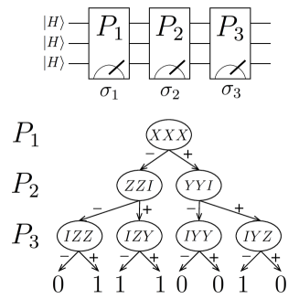
Figure 1: Example of a PBC on $n=3$ qubits. Each step $t$ involves an eigenvalue measurement of a Pauli operator $P_{t}$ on $n$ qubits with an outcome $\sigma_{t}=\pm 1$. A choice of $P_{t}$ may depend on the outcomes of all previous measurements. A PBC on $n$ qubits can be described by a binary tree ${\mathcal{T}}$ of height $n$ such that internal nodes of ${\mathcal{T}}$ are labeled by $n$-qubit Pauli operators and leaves of ${\mathcal{T}}$ are labeled by $0$ and $1$. The latter represent the final output bit $b_{out}$. We require that label of any node of ${\mathcal{T}}$ can be computed classically in time $poly(n)$.

Once all Pauli operators $P_{1},\ldots,P_{n}$ have been measured, the final quantum state is discarded and one is left with a list of measured eigenvalues $\sigma_{1},\ldots,\sigma_{n}$. The outcome of a PBC is a single classical bit $b_{out}$ obtained by performing a classical processing of the measured eigenvalues. All classical processing must take time at most $poly(n)$. We shall prove that the computational power of a PBC does not change if one additionally requires that all Pauli operators $P_{1},\ldots,P_{n}$ pairwise commute (for all measurement outcomes). A classical or quantum algorithm is said to simulate a PBC if it computes probability of the output $b_{out}=1$ with a small additive error. An example of a PBC is shown at Fig. 1.

The PBC model naturally appears in fault-tolerant quantum computing schemes based on error correcting codes of stabilizer type Gottesman (1998). Such codes enable a simple fault-tolerant implementation of non-destructive Pauli measurements on encoded qubits, for example using the Steane method Steane (1997). Furthermore, topological quantum codes such as the surface code enable a direct measurement of certain logical Pauli operators by measuring a properly chosen subset of physical qubits Fowler et al. (2009). Several fault-tolerant protocols for preparing encoded magic states such as $|H\rangle$ have been developed Bravyi and Kitaev (2005); Meier et al. (2012); Bravyi and Haah (2012); Jones (2013); Fowler et al. (2013). PBCs implicitly appeared in the previous work on quantum fault-tolerance. Our analysis closely follows the work by Campbell and Brown Campbell and Browne (2009) who showed that a certain class of magic state distillation protocols can be implemented by PBCs.

Let us now state our results. First, we claim that a PBC has the same computational power as the standard circuit-based quantum computing model.

Theorem 2.

Any quantum computation in the circuit-based model with $n$ qubits and $poly(n)$ gates drawn from the Clifford+T set can be simulated by a PBC on $m$ qubits, where $m$ is the number of $T$ gates, and $poly(n)$ classical processing.

Recall that the Clifford+T gate set consists of single-qubit gates

$$H=\frac{1}{\sqrt{2}}\left[\begin{array}[]{cc}1&1\\ 1&-1\\ \end{array}\right],\quad S=\left[\begin{array}[]{cc}1&0\\ 0&i\\ \end{array}\right],\quad T=\left[\begin{array}[]{cc}1&0\\ 0&e^{i\pi/4}\\ \end{array}\right],$$

and the two-qubit CNOT gate. This gate set is known to be universal for quantum computing. Secondly, we show that PBCs enable efficient addition of virtual qubits.

Theorem 3.

A PBC on $n+k$ qubits can be simulated by a PBC on $n$ qubits repeated $2^{O(k)}$ times and a classical processing which takes time $2^{O(k)}poly(n)$.

Both theorems follow from the fact that a generalized PBC that incorporates unitary Clifford gates, ancillary stabilizer states (such as $|0\rangle$ or $|+\rangle$), and has $poly(n)$ measurements can be efficiently simulated by the standard PBC defined above. To prove Theorem 2 we convert a given quantum circuit on $n$ qubits with $m$ $T$-gates into a generalized PBC on $n+m$ qubits initialized in the $|0^{\otimes n}\rangle\otimes|H^{\otimes m}\rangle$ state. Each $T$-gate of the circuit is converted into a simple gadget that includes adaptive Pauli measurements and consumes one copy of the $|H\rangle$ state. Simulating such generalized PBC by the standard PBC on $m$ qubits proves Theorem 2.

To prove Theorem 3 we represent $k$ copies of the magic state $|H\rangle$ as a linear combination of $k$-qubit stabilizer states $\phi_{\alpha}$ such that $|H\rangle\langle H|^{\otimes k}=\sum_{\alpha}c_{\alpha}|\phi_{\alpha}\rangle\langle\phi_{\alpha}|$ for some real coefficients $c_{\alpha}$. The number of terms in this sum is $2^{O(k)}$. We carry out the simulation independently for each $\alpha$ using a generalized PBC on $k+n$ qubits initialized in the state $|\phi_{\alpha}\rangle\otimes|H^{\otimes n}\rangle$ and combine the outcomes on a classical computer. Finally, we simulate the generalized PBCs by the standard PBCs on $n$ qubits.

Perhaps more surprisingly, we prove that PBCs can be simulated on a classical computer alone more efficiently than one could expect naively. Let us first describe a brute-force simulation method based on the matrix-vector multiplication. Let $\phi_{t}$ be the $n$-qubit state obtained after measuring the Pauli operators $P_{1},\ldots,P_{t}$. One can store $\phi_{t}$ in a classical memory as a complex vector of size $2^{n}$. Each step of a PBC involves a transformation $\phi_{t}\to\phi_{t+1}$ where $\phi_{t+1}=(1/2)(I+\sigma_{t}P_{t})\phi_{t}$. Since $P_{t}$ is a Pauli operator, the matrix of $P_{t}$ in the standard basis is a permutation matrix modulo phase factors. Thus, for a fixed vector $\phi_{t}$, one can compute $\phi_{t+1}$ for both choices of $\sigma_{t}$ in time $O(2^{n})$. Furthermore, one can compute the norm of $\phi_{t+1}$ in time $O(2^{n})$ and thus determine the probability of each measurement outcome $\sigma_{t}$. By flipping a classical coin one can generate a random variable $\sigma_{t}=\pm 1$ with the desired probability distribution. Since any PBC has at most $n$ steps, the overall cost of the classical simulation is $O(n2^{n})$. Below we show that this brute force simulation method is not optimal.

Theorem 4.

Any PBC on $n$ qubits can be simulated classically in time $2^{\alpha n}poly(n)$, where $\alpha\approx 0.94$.

Our simulation algorithm exploits the fact that tensor products of magic states admit a low-rank decomposition into stabilizer states. Recall that an $n$-qubit state $\phi$ is called a stabilizer state if $|\phi\rangle=U|0^{\otimes n}\rangle$ for some $n$-qubit Clifford operator $U$ — a product of the elementary gates $H$, $S$, and the CNOT.

Suppose $\psi$ is an arbitrary $n$-qubit state. Define a stabilizer rank of $\psi$ as the smallest integer $\chi$ such that $\psi$ can be written as $|\psi\rangle=\sum_{\alpha=1}^{\chi}c_{\alpha}|\phi_{\alpha}\rangle$, where $c_{\alpha}$ are complex coefficients and $\phi_{\alpha}$ are $n$-qubit stabilizer states. The stabilizer rank of $\psi$ will be denoted $\chi(\psi)$. By definition, $1\leq\chi(\psi)\leq 2^{n}$ for any $n$-qubit state $\psi$ and $\chi(\psi)=1$ iff $\psi$ is a stabilizer state. For example, the magic state $|H\rangle$ has stabilizer rank $\chi(H)=2$, since $|H\rangle$ is not a stabilizer state itself, but it can be written as a linear combination of two stabilizer states $|0\rangle$ and $|1\rangle$. Furthermore, using the identity

$$|H^{\otimes 2}\rangle=\frac{1}{2}(|00\rangle+|11\rangle)+\frac{1}{2\sqrt{2}}(|00\rangle+|01\rangle+|10\rangle-|11\rangle)$$

one can easily check that $\chi(H^{\otimes 2})=2$. More generally, let $\chi_{n}$ be the stabilizer rank of $|H^{\otimes n}\rangle$. Note that $\chi_{n+m}\leq\chi_{n}\chi_{m}$ since a tensor product of two stabilizer states is a stabilizer state. In particular, $\chi_{n}\leq(\chi_{2})^{n/2}=2^{n/2}$.

The probability to observe measurement outcomes $\sigma_{1},\ldots,\sigma_{t}$ in a PBC implemented up to a step $t$ can be written as

$$\langle H^{\otimes n}|\Pi|H^{\otimes n}\rangle=\sum_{\alpha,\beta=1}^{\chi_{n}}\overline{c}_{\alpha}c_{\beta}\langle\phi_{\alpha}|\Pi|\phi_{\beta}\rangle$$

where $\phi_{\alpha}$ are $n$-qubit stabilizer states, $c_{\alpha}$ are complex coefficients, and $\Pi=\prod_{a=1}^{t}(I+\sigma_{a}P_{a})/2$ is the projector describing the partially implemented PBC. We will use a version of the Gottesman-Knill theorem Aaronson and Gottesman (2004) to show that each term $\langle\phi_{\alpha}|\Pi|\phi_{\beta}\rangle$ can be computed on a classical computer in time $n^{3}$. Since the number of terms is $\chi_{n}^{2}$ and the number of steps is at most $n$, we would be able to simulate a PBC on $n$ qubits classically in time $(\chi_{n})^{2}n^{4}$. Improving upon the brute-force simulation method thus requires an upper bound $\chi_{n}\leq 2^{\beta n}$ for some $\beta<1/2$. We establish such an upper bound with $\beta=\log_{2}{(7)}/6\approx 0.468$ by showing that $\chi_{6}\leq 7$ which implies $\chi_{n}\leq(\chi_{6})^{n/6}\leq 7^{n/6}$. We expect that the scaling in Theorem 4 can be improved by computing $\chi_{n}$ for larger values of $n$. In Appendix B we describe a heuristic algorithm for computing low-rank decompositions of $|H^{\otimes n}\rangle$ into stabilizer states which yields the following upper bounds:

$n$	$\;2\;$	$\;3\;$	$\;4\;$	$\;5\;$	$\;6\;$
$\chi_{n}\leq$	$2$	$3$	$4$	$6$	$7$

We believe that these upper bounds are tight. A lower bound $\chi_{n}\geq\Omega(n^{1/2})$ is proved in Appendix C.

II Discussion and previous work

Classical algorithms for simulation of quantum circuits based on the stabilizer formalism have a long history. Notably, Aaronson and Gottesman Aaronson and Gottesman (2004) studied adaptive quantum circuits that contain only a few non-Clifford gates. Assuming that a circuit contains at most $m$ non-Clifford gates and that all $n$ qubits are initially prepared in some stabilizer state, Ref. Aaronson and Gottesman (2004) showed how to simulate such a circuit classically in time $2^{4m}poly(n)$. To enable a comparison with our results, assume that all unitary gates belong to the Clifford+$T$ set. By Theorem 2, a quantum circuit as above can be transformed into a PBC on $m$ qubits, where $m$ is the number of $T$-gates. Thus Theorems 2,4 provide a classical simulation algorithm with a running time $2^{0.94m}poly(n)$ which improves upon Aaronson and Gottesman (2004). In addition, Ref. Aaronson and Gottesman (2004) studied adaptive quantum circuits composed only of Clifford gates and Pauli measurements with more general initial states. Assuming that the initial $n$-qubit state can be written as a tensor product of some $b$-qubit states, a quantum circuit as above can be simulated classically in time $2^{2b+2d}poly(n)$, where $d$ is the total number of measurements Aaronson and Gottesman (2004).

Methods for decomposing arbitrary states into a linear combination of stabilizer states aimed at simulation of quantum circuits were pioneered by Garcia, Markov, and Cross Garcia et al. (2012); García et al. (2014) who studied decompositions into pairwise orthogonal stabilizer states (named stabilizer frames). The latter are more restrictive than the general decompositions analyzed in the present paper. Furthermore, Refs. Garcia et al. (2012); García et al. (2014) have not studied stabilizer decompositions of magic states.

The simulation algorithm of Theorem 4 is conceptually close to the matrix multiplication algorithms based on tensor decompositions Strassen (1969); Coppersmith and Winograd (1987). In this case the analogue of a stabilizer state is a product state and the analogue of a magic state is a tripartite entangled state that contains EPR-type states shared between each pair of parties, see Chitambar et al. (2008) for details.

Efficient classical algorithms for simulation of quantum circuits in which the initial state can be described by a discrete Wigner function taking non-negative values were investigated by Veitch et al Veitch et al. (2012) and by Howard Howard et al. (2014) et al. As was pointed out by Pashayan, Wallman, and Bartlett Pashayan et al. (2015), such methods can be combined with Monte Carlo sampling techniques to enable classical simulation of general quantum circuits with the running time scaling exponentially with the quantity related to the negativity of the Wigner function. To enable a comparison between Theorem 4 and the results of Pashayan et al. (2015) one can employ a discrete Wigner function representation of stabilizer states and Clifford operations on qubits developed by Delfosse et al Delfosse et al. (2014). The latter is applicable only to states with real amplitudes and to Clifford operations that do not mix $X$-type and $Z$-type Pauli operators (CSS-preserving operations). A preliminary analysis shows that combining the results of Refs. Pashayan et al. (2015); Delfosse et al. (2014) yields a classical algorithm for simulating a restricted class of PBC on $n$ qubits in time $M^{2n}poly(n)\approx 2^{0.543n}poly(n)$, where $M=2^{-1}+2^{-1/2}\approx 1.207$ is the so-called mana of the magic state $|H\rangle\langle H|$, see Pashayan et al. (2015); Delfosse et al. (2014) for details. The restriction is that all Pauli operators to be measured are either $X$-type or $Z$-type, and the measurements cannot be adaptive. Such restricted PBCs are not known to be universal for quantum computation.

Our method of simulating sparse quantum circuits has connections to ideas of tensor network representations of quantum circuits developed by Markov and Shi Markov and Shi (2008). Indeed, our proof of Theorem 1 can be interpreted as a particular method of expressing the acceptance probability of a quantum computation in terms of a contraction of tensors associated with the quantum circuit. The individual entries of the tensors are then estimated separately with a smaller quantum computer and then added together.

Let us now discuss some open problems and possible generalizations of our work. A natural question is whether the scaling in Theorem 4 can be improved if $|H\rangle$ is replaced by some other magic state. By definition, any magic state is Clifford-equivalent to one of the states $|H\rangle$ and $|R\rangle$, where $|R\rangle$ is the $+1$ eigenvector of an operator $(X+Y+Z)/\sqrt{3}$, see Ref. Bravyi and Kitaev (2005) for details. The numerics suggests that $|H^{\otimes n}\rangle$ and $|R^{\otimes n}\rangle$ have the same stabilizer rank for $n\leq 6$. We conjecture that this remains true for all $n$. Moreover, we pose the following conjecture which, if true, highlights a new optimality property of magic states in terms of their stabilizer rank.

Conjecture 1.

Let $\chi_{n}$ be the stabilizer rank of $|H^{\otimes n}\rangle$ and $\phi$ be an arbitrary single-qubit state. Then

$$\chi(\phi^{\otimes n})=1 \mbox{if $\phi$ is a stabilizer state},$$

$$\chi(\phi^{\otimes n})=\chi_{n} \mbox{if $\phi$ is a magic state},$$

$$\chi(\phi^{\otimes n})>\chi_{n} \mbox{otherwise}.$$

Less formally, the conjecture says that magic states have the smallest possible stabilizer rank among all non-stabilizer single-qubit states.

It is also of great interest to understand the asymptotic scaling of the stabilizer rank $\chi_{n}$. Assuming that a universal quantum computation cannot be simulated classically in polynomial time, one infers that $\chi_{n}$ must grow super-polynomially in the limit $n\to\infty$. However, we were unable to derive such a lower bound directly without using any assumptions. The fact that amplitudes of any stabilizer state in the standard basis take only $O(1)$ different values implies a weaker lower bound $\chi_{n}\geq\Omega(n^{1/2})$, see Appendix C. We conjecture that in fact $\chi_{n}\geq 2^{\Omega(n)}$. Note that if this conjecture is false, that is, $\chi_{n}\leq 2^{o(n)}$, then constant-depth circuits in the Clifford+$T$ basis can be simulated classically in a sub-exponential time, which appears unlikely. Indeed, since such a circuit contains at most $m=O(n)$ $T$-gates, where $n$ is the number of qubits, Theorems 2,4 would provide a simulation algorithm with a running time $\chi_{m}^{2}\cdot poly(n)=2^{o(n)}poly(n)$. (Here we ignore the complexity of finding the optimal stabilizer decomposition since it has to be done only once for each $n$.)

Finally, one may explore generalizations of the stabilizer rank to approximate decompositions into stabilizer states. It should be pointed out that the simulation algorithm of Theorem 4 would require approximate stabilizer decompositions with a precision at least $2^{-\Omega(n)}$ since the probability of a particular measurement outcome $\sigma_{1},\ldots,\sigma_{t}$ can be exponentially small in $n$. It is not clear whether such approximate decompositions would have a rank substantially smaller than the exact ones.

In the rest of the paper we prove the theorems stated in the introduction. From the technical perspective, Theorems 1,2,3 follow easily from the definitions and from the previously known results. On the other hand, Theorem 4 and the notion of a stabilizer rank appear to be new. We analyze sparse quantum circuits in Section III. A classical algorithm for simulation of PBCs and the stabilizer rank of magic states are discussed in Section IV. Theorems 2,3 are proved in Section V. Appendix A proves a technical lemma needed to compute inner products between stabilizer states. Appendix B describes a numerical method of computing low-rank stabilizer decompositions. Appendix C proves a lower bound on the stabilizer rank of magic states.

III Sparse quantum circuits

In this section we prove Theorem 1. All quantum circuits considered below are defined with respect to some fixed basis of gates $\mathcal{G}$. We assume that any gate in $\mathcal{G}$ acts on at most two qubits. Furthermore, we assume that $\mathcal{G}$ contains all single-qubit Pauli gates $X,Y,Z$, their controlled versions, the Hadamard gate, and the $\pi/2$ phase shift $S=|0\rangle\langle 0|+i|1\rangle\langle 1|$. For example, $\mathcal{G}$ could be the Clifford+$T$ basis. Let $\Sigma^{n}\equiv\{0,1\}^{n}$ be the set of $n$-bit binary strings.

Lemma 1.

Let $U$ be a $d$-sparse quantum circuit on $k+n$ qubits. Partition the set of qubits as $AB$, where $|A|=k$ and $|B|=n$. Then

$$U=\sum_{\alpha=1}^{\chi}c_{\alpha}V_{\alpha}\otimes W_{\alpha},\quad\quad\chi\equiv 2^{4kd},$$ (1)

where $V_{\alpha}$ and $W_{\alpha}$ are $d$-sparse quantum circuit acting on $A$ and $B$ respectively, and $c_{\alpha}$ are some complex coefficients such that $\sum_{\alpha=1}^{\chi}|c_{\alpha}|^{2}=1$.

Proof.

Since $U$ is a $d$-sparse circuit, it contains at most $kd$ two-qubit gates that couple some qubit of $A$ and some qubit of $B$. Let $G_{1},\ldots,G_{m}$ be the list of all such gates, where $m\leq kd$. Any two-qubit gate $G[i,j]$ acting on qubits $i\in A$ and $j\in B$ can be expanded in the Pauli basis as $G[i,j]=\sum_{\alpha=1}^{16}c_{\alpha}P_{\alpha}[i]\otimes P_{\alpha}[j]$, where $P_{\alpha}\in\{I,X,Y,Z\}$ are Pauli operators and $c_{\alpha}$ are some complex coefficients such that $\sum_{\alpha}|c_{\alpha}|^{2}=1$. Applying the above decomposition to each gate $G_{1},\ldots,G_{m}$ and, if necessary, appending dummy identity gates to make $m=kd$, one arrives at Eq. (1). Note that replacing a two-qubit gate in $U$ by a tensor product of two single-qubit Pauli gates cannot increase the sparsity of the circuit. Thus each term $V_{\alpha}\otimes W_{\alpha}$ is a tensor product of two $d$-sparse circuits. ∎

The classical post-processing step can be described by a $poly(n)$ classical circuit $f\,:\,\Sigma^{n+k}\to\{0,1\}$. By definition of the SQC model, the final output of a computation is a single random bit $b_{out}=f(x)$, where $x\in\Sigma^{n+k}$ is the bit string obtained by measuring each qubit of a state $U|0^{n+k}\rangle$ in the $0,1$ basis. Let $\pi(U)$ be the probability of the output $b_{out}=1$, that is,

$$\pi(U)=\langle 0^{n+k}|U^{\dagger}\Pi U|0^{n+k}\rangle,$$

$$\Pi=\sum_{x\,:\,f(x)=1}|x\rangle\langle x|.$$ (2)

Let us first show how to estimate the quantity $\pi(U)$ with a small additive error using $dk$-sparse circuits on $n+1$ qubits. Substituting Eq. (1) into the definition of $\pi(U)$ one gets

$$\pi(U)=\sum_{y\in\Sigma^{k}}\sum_{\alpha,\beta=1}^{\chi}c_{\alpha}(y)\overline{c_{\beta}(y)}\langle\phi_{\alpha}|\Pi(y)|\phi_{\beta}\rangle,$$ (3)

where

$$c_{\alpha}(y)=c_{\alpha}\langle y|V_{\alpha}|0^{k}\rangle,\quad\quad|\phi_{\alpha}\rangle=W_{\alpha}|0^{n}\rangle,$$

and

$$\Pi(y)=\sum_{\begin{subarray}{c}z\in\Sigma^{n}\\ f(yz)=1\\ \end{subarray}}\;|z\rangle\langle z|.$$

We claim that each coefficient $c_{\alpha}(y)$ can be computed exactly in time $O(kd\cdot 2^{k})$. Indeed, we can merge consecutive single-qubit gates of $V_{\alpha}$ such that each qubit is acted upon by at most $d$ two-qubit gates and at most $d+1$ single-qubit gates. Thus we can assume that the total number of gates in $V_{\alpha}$ is $O(kd$). One can compute the quantity $\langle y|V_{\alpha}|0^{k}\rangle$ classically in time $O(kd\cdot 2^{k})$ by performing matrix-vector multiplication for each gate of $V_{\alpha}$. Furthermore, it is clear from the proof of Lemma 1 that each coefficient $c_{\alpha}$ can be computed in time $O(kd)$.

Consider some fixed triple $(y,\alpha,\beta)$ that appears in the sum Eq. (3). Define a controlled-$W$ operator

$$\Lambda(W)=|0\rangle\langle 0|\otimes W_{\alpha}+|1\rangle\langle 1|\otimes W_{\beta}.$$

Define a quantum circuit $R$ acting on $n+1$ qubits that consists of the following steps: (i) initialize $n+1$ qubits in the $|0\rangle$ state, (ii) apply $H$ gate to the first qubit, (iii) apply $\Lambda(W)$ with the first qubit acting as the control one, (iv) apply $H$ gate to the first qubit, (v) measure each qubit in the $0,1$-basis. The construction of $R$, illustrated at Fig. 2, is very similar to the standard SWAP test, except that we finally measure each qubit. Let $b,z$ be the measurement outcomes, where $b=0,1$ and $z\in\Sigma^{n}$, see Fig. 2. Define a random variable $\sigma^{\prime}_{y,\alpha,\beta}$ taking values $\pm 1$ such that $\sigma^{\prime}_{y,\alpha,\beta}=1$ iff $b=0$ and $f(yz)=1$. Otherwise $\sigma^{\prime}_{y,\alpha,\beta}=-1$. A simple algebra shows that

$$\mathrm{Re}(\langle\phi_{\alpha}|\Pi(y)|\phi_{\beta}\rangle)=\mathbb{E}(\sigma^{\prime}_{y,\alpha,\beta}),$$ (4)

that is $\sigma^{\prime}_{y,\alpha,\beta}$ is an unbiased estimator of the real part of $\langle\phi_{\alpha}|\Pi(y)|\phi_{\beta}\rangle$. We claim that one can get a sample of $\sigma^{\prime}_{y,\alpha,\beta}$ by executing a single instance of a $dk$-sparse quantum computation on $n+1$ qubits (with certain special properties). Indeed, by construction, the circuits $W_{\alpha}$ and $W_{\beta}$ can be obtained from each other by changing some subset of at most $kd$ single-qubit Pauli gates. Thus the controlled circuit $\Lambda(W)$ only needs control for at most $kd$ single-qubit Pauli gates. This shows that the control qubit participates in at most $kd$ two-qubit gates. Furthermore, since all locations where $W_{\alpha}$ and $W_{\beta}$ differ from each other originate from two-qubit gates in the initial $d$-sparse circuit $U$, we conclude that the circuit $R$ has a special property that all qubits except for the control one participate in at most $d$ two-qubit gates. One can similarly define a random variable $\sigma^{\prime\prime}_{y,\alpha,\beta}$ such that

$$\mathrm{Im}(\langle\phi_{\alpha}|\Pi(y)|\phi_{\beta}\rangle)=\mathbb{E}(\sigma^{\prime\prime}_{y,\alpha,\beta}).$$

The only difference is that the $H$ gate in the circuit $R$ must be replaced by $HS$ gate. We conclude that

$$\langle\phi_{\alpha}|\Pi(y)|\phi_{\beta}\rangle=\mathbb{E}(\sigma^{\prime}_{y,\alpha,\beta})+i\mathbb{E}(\sigma^{\prime\prime}_{y,\alpha,\beta}).$$

Thus the quantity $\pi(U)$ has an unbiased estimator

$$\xi\equiv\sum_{y\in\Sigma^{k}}\sum_{\alpha,\beta=1}^{\chi}c_{\alpha}(y)\overline{c_{\beta}(y)}\left(\sigma^{\prime}_{y,\alpha,\beta}+i\sigma^{\prime\prime}_{y,\alpha,\beta}\right),$$

that is, $\pi(U)=\mathbb{E}(\xi)$. Using the bounds $|c_{\alpha}(y)|\leq|c_{\alpha}|$ and $\sum_{\alpha=1}^{\chi}|c_{\alpha}|^{2}=1$ one gets

$$|\xi|\leq 2\sum_{y\in\Sigma^{k}}\sum_{\alpha,\beta=1}^{\chi}|c_{\alpha}(y)\overline{c_{\beta}(y)}|\leq 2^{k+1}\chi$$

with probability one. By Hoeffding’s inequality, one can estimate $\mathbb{E}(\xi)$ with a small additive error by generating $c2^{2k}\chi^{2}$ samples of $\xi$ for some constant $c=O(1)$. Generating each sample of $\xi$ requires $2^{k}\chi^{2}$ samples of the $\sigma$-variables. Thus one can estimate $\pi(U)$ by repeated applications of $dk$-sparse circuits on $n+1$ qubits with the number of repetitions scaling as $c2^{3k}\chi^{4}=c2^{16kd+3k}=2^{O(kd)}$.

Recall that the $dk$-sparse circuits $R$ constructed above have a very special pattern of sparsity. Namely, all qubits except for one participate in at most $d$ two-qubit gates, whereas one remaining qubit participates in at most $kd$ two-qubit gates. We can distribute the sparsity more evenly among all $n+1$ qubits by performing a swap gate that changes position of the control qubit after each application of a control gate (this is possible only if $n$ is sufficiently large, specifically, if $n\geq kd+1$). After this modification one obtains an equivalent circuit which is $(d+3)$-sparse.

Finally, we can apply exactly the same arguments as above if the subsets $A$ and $B$ in Lemma 1 have size $|A|=k+1$ and $|B|=n-1$. This frees up one extra qubit that can play the role of the control one in the above construction. Now we can estimate $\pi(U)$ by repeated applications of $(d+3)$-sparse circuits on $n$ qubits with the number of repetitions scaling as $c2^{16(k+1)d+3(k+1)}=2^{O(kd)}$. This completes the proof of Theorem 1.

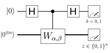
Figure 2: Quantum circuit $R$ used to estimate the real part of $\langle\phi_{\alpha}|\Pi(y)|\phi_{\beta}\rangle$ in Eq. (3). The final output of the circuit is a random variable $\sigma^{\prime}_{y,\alpha,\beta}=\pm 1$ such that $\sigma^{\prime}_{y,\alpha,\beta}=1$ iff $b=0$ and $f(yz)=1$, where $f\,:\,\{0,1\}^{n+k}\to\{0,1\}$ is the Boolean function describing post-processing step in the original circuit $U$ on $n+k$ qubits. We construct a circuit $R$ as above for each triple $(y,\alpha,\beta)$ with $y\in\{0,1\}^{k}$ and $\alpha,\beta=1,\ldots,\chi$. A simple algebra shows that $\sigma^{\prime}_{y,\alpha,\beta}$ is an unbiased estimator of $\mathrm{Re}(\langle\phi_{\alpha}|\Pi(y)|\phi_{\beta}\rangle)$.

IV Stabilizer rank and classical simulation of PBC

In this section we prove Theorem 4. We begin with an algorithm for computing a quantity $\langle\psi|\Pi|\phi\rangle$, where $\psi,\phi$ are $n$-qubit stabilizer states and $\Pi$ is a projector onto the codespace of some stabilizer code. We note that several previous works addressed the problem of computing the inner product $\langle\psi|\phi\rangle$ between stabilizer states $\psi,\phi$. In particular, Aaronson and Gottesman Aaronson and Gottesman (2004) showed that the magnitude $|\langle\psi|\phi\rangle|$can be computed in time $O(n^{3})$. Furthermore, Garcia, Markov, and Cross García et al. (2014) used canonical form of Clifford circuits to compute both the magnitude and the phase of $\langle\psi|\phi\rangle$ in time $O(n^{3})$. Below we describe a technically different (and somewhat simpler) algorithm which is more suited for computing the quantity $\langle\psi|\Pi|\phi\rangle$ as above.

Let $\mathbb{Z}_{m}\equiv\{0,1,\ldots,m-1\}$ be the cyclic group of order $m$. A function $f\,:\,\mathbb{F}_{2}^{n}\to\mathbb{Z}_{8}$ is called a degree-two polynomial if

$$f(x_{1},\ldots,x_{n})=f_{\emptyset}+2\sum_{a=1}^{n}f_{a}x_{a}+4\sum_{1\leq a<b\leq n}f_{a,b}x_{a}x_{b}$$

where $f_{\emptyset}\in\mathbb{Z}_{8}$, $f_{a}\in\mathbb{Z}_{4}$, and $f_{a,b}\in\mathbb{Z}_{2}$ are some constant coefficients. Define

$$\langle f\rangle=\sum_{x\in\mathbb{F}_{2}^{n}}\omega^{f(x)},\quad\quad\omega\equiv e^{i\pi/4}.$$

Lemma 2.

Let $f\,:\,\mathbb{F}_{2}^{n}\to\mathbb{Z}_{8}$ be a degree-two polynomial. Then either $\langle f\rangle=0$ or $\langle f\rangle=2^{p/2}\omega^{m}$ for some integer $n\leq p\leq 2n$ and some $m\in\mathbb{Z}_{8}$. Furthermore, one can compute $\langle f\rangle$ in time $O(n^{3})$.

Since the proof is rather straightforward, we postpone it until Appendix A. It was shown by Dehaene and De Moor Dehaene and De Moor (2003) and by Van den Nest Van den Nest (2010) that any stabilizer state $\psi$ of $n$-qubit can be written (up to a global phase and a normalization) as

$$|\psi\rangle=\sum_{u\in\mathbb{F}_{2}^{k}}\omega^{f(u)}|z+u\Psi\rangle,$$ (5)

for some degree-two polynomial $f\,:\,\mathbb{F}_{2}^{k}\to\mathbb{Z}_{8}$, some $k\times n$ binary matrix $\Psi$, and some vector $z\in\mathbb{F}_{2}^{n}$. Here we treat $u$ and $z$ as row vectors. In the rest of this section we take Eq. (5) as our definition of a stabilizer state.

Let $\mathcal{G}\subset{\mathcal{P}}^{n}$ be an abelian group with $t$ independent generators $P_{1},P_{2},\ldots,P_{t}\in\mathcal{G}$. Define a projector $\Pi$ onto the $\mathcal{G}$-invariant subspace,

$$\Pi=2^{-t}\sum_{P\in\mathcal{G}}P.$$

Lemma 3.

The action of $\Pi$ in the computational basis can be represented as

$$\Pi|x\rangle=2^{-t}\sum_{y\in\mathbb{F}_{2}^{t}}\omega^{g(y)}(-1)^{yBx^{T}}|x+yA\rangle$$

for some degree-two polynomial $g\,:\,\mathbb{F}_{2}^{t}\to\mathbb{Z}_{8}$ and some binary matrices $A,B$ of size $t\times n$.

Proof.

Given a binary vector $f\in\mathbb{F}_{2}^{n}$, let $X(f)\in{\mathcal{P}}^{n}$ be the Pauli operator that applies $X$ to each qubit in the support of $f$. Define $Z(f)$ in a similar fashion. Let $e^{k}\in\mathbb{F}_{2}^{t}$ be the basis vector which has a single ‘1’ at the position $k$. The $k$-th generator of $\mathcal{G}$ can be written as $P_{k}=i^{c_{k}}X(e^{k}A)Z(e^{k}B)$ for some $c_{k}\in\mathbb{Z}_{4}$ and some binary matrices $A,B$ of size $t\times n$. In other words, the $k$-th row of $A$ (of $B$) specifies the $X$-part (the $Z$-part) of $P_{k}$. Choose any vector $y\in\mathbb{F}_{2}^{t}$. Then

$$P(y)\equiv\prod_{k\,:\,y_{k}=1}P_{k}=\omega^{g(y)}X(yA)Z(yB),$$

where

$$\omega^{g(y)}=i^{\sum_{k=1}^{t}c_{k}y_{k}}\cdot(-1)^{\sum_{1\leq k<l\leq t}(BA^{T})_{k,l}y_{k}y_{l}}.$$

Clearly, $g\,:\,\mathbb{F}_{2}^{t}\to\mathbb{Z}_{8}$ is a degree-two polynomial. Thus

$$2^{t}\Pi|x\rangle=\sum_{y\in\mathbb{F}_{2}^{t}}P(y)|x\rangle=\sum_{y\in\mathbb{F}_{2}^{t}}\omega^{g(y)}(-1)^{yBx^{T}}|x+yA\rangle.$$

∎

Consider now a pair of $n$-qubit stabilizer states $\psi,\phi$, where $\psi$ is defined in Eq. (5) and

$$|\phi\rangle=\sum_{v\in\mathbb{F}_{2}^{m}}\omega^{h(v)}|z^{\prime}+v\Phi\rangle.$$ (6)

Here $h\,:\,\mathbb{F}_{2}^{m}\to\mathbb{Z}_{8}$ is a degree-two polynomial, $\Phi$ is a binary matrix of size $m\times n$, and $z^{\prime}\in\mathbb{F}_{2}^{n}$ is some vector. Using Lemma 3 and Eqs. (5,6) one gets

$$\langle\psi|\Pi|\phi\rangle =2^{-t}\sum_{u,v,y}\omega^{h(v)-f(u)+g(y)}$$

$$\cdot(-1)^{yB(z^{\prime}+v\Phi)^{T}}\langle z+u\Psi|z^{\prime}+v\Phi+yA\rangle.$$

Clearly the non-zero terms are those with $z+u\Psi=z^{\prime}+v\Phi+yA$. We can enforce this equality by introducing an extra variable $x\in\mathbb{F}_{2}^{n}$ such that

$$\langle z+u\Psi|z^{\prime}+v\Phi+yA\rangle=2^{-n}\sum_{x\in\mathbb{F}_{2}^{n}}(-1)^{x(z+u\Psi+z^{\prime}+v\Phi+yA)}.$$

Then

$$\langle\psi|\Pi|\phi\rangle=2^{-n+t}\sum_{u,v,x,y}\omega^{F(u,v,x,y)}=2^{-n+t}\langle F\rangle$$ (7)

with

$$F(u,v,x,y) =h(v)-f(u)+g(y)+4yB(z^{\prime}+v\Phi)^{T}$$

$$+4x(z+u\Psi+z^{\prime}+v\Phi+yA).$$

Note that $F(u,v,x,y)$ is a degree-two polynomial in $k+m+n+t$ variables. By Lemma 2, one can compute the sum $\langle F\rangle$ in time $O(k+m+t+n)^{3}=O(n^{3})$. Also, Lemma 2 and Eq. (7) implies that $\langle\psi|\Pi|\phi\rangle$ takes values $2^{q/2}\omega^{j}$ for some integer $q$ and $j\in\mathbb{Z}_{8}$.

Consider now a PBC on $n$ qubits as defined in Section V. Let $t$ be some fixed time step. Recall that a sequence of measurement outcomes $\sigma_{1},\ldots,\sigma_{t}$ is observed with the probability

$$\mathrm{Pr}(\sigma_{1},\ldots,\sigma_{t})=\langle H^{\otimes n}|\prod_{k=1}^{t}(1/2)(I+\sigma_{k}P_{k})|H^{\otimes n}\rangle.$$

Below we shall construct an algorithm that takes as input a step $t$, a sequence of outcomes $\sigma_{1},\ldots,\sigma_{t}$ and returns $\mathrm{Pr}(\sigma_{1},\ldots,\sigma_{t})$. It allows us to compute $\mathrm{Pr}(\sigma_{1})$ and get a sample of $\sigma_{1}$ by flipping a coin with a properly chosen bias. By calling the algorithm twice one can also compute conditional probabilities

$$\mathrm{Pr}(\sigma_{t}|\sigma_{1},\ldots,\sigma_{t-1})=\frac{\mathrm{Pr}(\sigma_{1},\ldots,\sigma_{t})}{\mathrm{Pr}(\sigma_{1},\ldots,\sigma_{t-1})}.$$

Thus, for fixed variables $\sigma_{1},\ldots,\sigma_{t-1}$ one can get a sample of $\sigma_{t}$ by computing the conditional probability $\mathrm{Pr}(\sigma_{t}|\sigma_{1},\ldots,\sigma_{t-1})$ and flipping a coin with a properly chosen bias. The ability to sample the outcomes $\sigma_{1},\ldots,\sigma_{n}$ from the distribution $\mathrm{Pr}(\sigma_{1},\ldots,\sigma_{n})$ is equivalent to simulating the PBC classically. Hence it suffices to construct an algorithm that computes $\mathrm{Pr}(\sigma_{1},\ldots,\sigma_{t})$.

Suppose we are given some integers $k,\chi=O(1)$ and a decomposition

$$|H^{\otimes k}\rangle=\sum_{\alpha=1}^{\chi}c_{\alpha}|\phi_{\alpha}\rangle$$ (8)

where $\phi_{a}$ are $k$-qubit stabilizer states and $c_{a}$ are complex coefficients. Suppose also that $n=mk$ for some integer $m$. Taking the $m$-fold tensor power of Eq. (8) one gets

$$|H^{\otimes n}\rangle=\sum_{\mathbf{a}=1}^{\chi^{m}}c_{\mathbf{a}}|{\phi}_{\mathbf{a}}\rangle,$$ (9)

where $\mathbf{a}=(\alpha_{1},\ldots,\alpha_{m})$, $c_{\mathbf{a}}=c_{\alpha_{1}}\cdots c_{\alpha_{m}}$, and ${\phi}_{\mathbf{a}}=\phi_{\alpha_{1}}\otimes\cdots\otimes\phi_{\alpha_{m}}$. Note that ${\phi}_{\mathbf{a}}$ are stabilizer states and for a given index $\mathbf{a}$ one can compute the standard form of ${\phi}_{\mathbf{a}}$ as defined in Eq. (5) in time $O(n)$. Denoting

$$\Pi=2^{-t}\prod_{k=1}^{t}(I+\sigma_{k}P_{k})$$

we get

$$\mathrm{Pr}(\sigma_{1},\ldots,\sigma_{t})=\sum_{\mathbf{a},\mathbf{b}=1}^{\chi^{m}}\overline{c_{\mathbf{a}}}c_{\mathbf{b}}\langle{\phi}_{\mathbf{a}}|\Pi|{\phi}_{\mathbf{{b}}}\rangle.$$ (10)

The discussion above implies that each term $\langle{\phi}_{\mathbf{a}}|\Pi|{\phi}_{\mathbf{b}}\rangle$ can be computed exactly in time $O(n^{3})$. Assuming that arithmetic operations with complex numbers have a unit cost (see Remark 1 below), the probability $\mathrm{Pr}(\sigma_{1},\ldots,\sigma_{t})$ can be computed in time $O(\chi^{2m}n^{3})=O(\chi^{2n/k}n^{3})$.

Let us now show an explicit decomposition Eq. (8) with $k=6$ and $\chi=7$. This gives an algorithm for computing $\mathrm{Pr}(\sigma_{1},\ldots,\sigma_{t})$ with a running time $O(7^{n/3}n^{3})$ which is enough to prove Theorem 4. It will be more convenient to normalize the magic state such that

$$|H\rangle=|0\rangle+t|1\rangle,\quad\quad t=\tan{(\pi/8)}=\sqrt{2}-1.$$

Let $B_{n}=\mathbb{F}_{2}^{n}$ be the set of all $n$-bit strings and $B_{n,k}\subset B_{n}$ be the subset of strings with the Hamming weight exactly $k$. Let $B_{n}=E_{n}\cup O_{n}$, where $E_{n}$ and $O_{n}$ are the subsets of even-weight and odd-weight strings respectively. Given a set of bit strings $S$, we shall write $|S\rangle=\sum_{x\in S}|x\rangle$ for the uniform superposition of all strings in $S$. For example, $|B_{n,0}\rangle=|0^{\otimes n}\rangle$, $|B_{n,n}\rangle=|1^{\otimes n}\rangle$, and $|H^{\otimes n}\rangle=\sum_{k=0}^{n}t^{k}|B_{n,k}\rangle$. Define also a state

$$|K_{n}\rangle=\sum_{x\in B_{n}}(-1)^{|x|(|x|-1)/2}\,|x\rangle=\prod_{i<j}\Lambda(Z)_{i,j}|B_{n}\rangle$$

Note that $|B_{n,0}\rangle$, $|B_{n,n}\rangle$, $|E_{n}\rangle$, $|O_{n}\rangle$, and $|K_{n}\rangle$ are stabilizer states as defined by Eq. (5). Define also a pair of graphs $G^{\prime}=(V^{\prime},E^{\prime})$ and $G^{\prime\prime}=(V^{\prime\prime},E^{\prime\prime})$ with six vertices shown on Fig. 3. The desired stabilizer decomposition of $|H^{\otimes 6}\rangle$ is

$$|H^{\otimes 6}\rangle = (-16+12\sqrt{2})|B_{6,0}\rangle+(96-68\sqrt{2})|B_{6,6}\rangle+(10-7\sqrt{2})|E_{6}\rangle+(-14+10\sqrt{2})|O_{6}\rangle$$ (11)

$$+(7-5\sqrt{2})Z^{\otimes 6}|K_{6}\rangle+(10-7\sqrt{2})|\phi^{\prime}\rangle+(10-7\sqrt{2})|\phi^{\prime\prime}\rangle.$$

where

$$|\phi^{\prime}\rangle=\prod_{(i,j)\in E^{\prime}}\Lambda(Z)_{i,j}|O_{6}\rangle\quad\mbox{and}\quad|\phi^{\prime\prime}\rangle=\prod_{(i,j)\in E^{\prime\prime}}\Lambda(Z)_{i,j}|O_{6}\rangle.$$

Figure 3: Graphs $G^{\prime}$ and $G^{\prime\prime}$ used in the definition of stabilizer states $\phi^{\prime}$ and $\phi^{\prime\prime}$, see Eq. (11).

This completes the proof of Theorem 4. The numerical method used to find the above decomposition is discussed in Appendix B. We conjecture that $k=6$ is the smallest integer such that $\chi_{k}^{2}<2^{k}$, see Section I. Accordingly, $k=6$ is likely to be the smallest integer for which the the above simulation strategy outperforms the brute-force simulation algorithm.

Remark 1: Let us point out that all coefficients in Eq. (11) belong to the ring $\mathbb{Z}[\sqrt{2}]=\{p+\sqrt{2}q\,:\,p,q\in\mathbb{Z}\}$ known the ring of quadratic integers with a base two. Hence the coefficients $c_{\mathbf{a}}$ in Eq. (9) also belong to $\mathbb{Z}[\sqrt{2}]$. Using Eq. (7) and Lemma 2 we conclude that each term in Eq. (10) has a form $2^{-q}\eta\omega^{j}$ for some integer $0\leq q\leq n$, some $\eta\in\mathbb{Z}[\sqrt{2}]$, and some $j\in\mathbb{Z}_{8}$. Multiplying Eq. (10) by a suitable power of two we can assume that each term in Eq. (10) has a form $\alpha+i\beta$ where $\alpha,\beta\in\mathbb{Z}[\sqrt{2}]$ (of course we can ignore the imaginary part $i\beta$ since $\mathrm{Pr}(\sigma_{1},\ldots,\sigma_{t})$ is a real number). Thus computing the sum in Eq. (10) only requires arithmetic operations in the ring $\mathbb{Z}[\sqrt{2}]$.

Remark 2: One can notice that the first five terms in Eq. (11) are stabilizer states symmetric under all permutations of qubits. On the other hand, the states $\phi^{\prime}$ and $\phi^{\prime\prime}$ break the permutation symmetry. Interestingly, we found that the state $|H^{\otimes 6}\rangle$ does not belong to the subspace spanned by symmetric stabilizer states of six qubits. Thus any stabilizer decomposition of $|H^{\otimes 6}\rangle$ must use at least two non-symmetric states. On the other hand, one can check that $|H^{\otimes n}\rangle$ belongs to the subspace spanned by symmetric stabilizer states for $n\leq 5$. The best decompositions that we were able to find for $n\leq 5$ are formed by symmetric stabilizer states, see Appendix B.

V Adding virtual qubits to a PBC

In this section we prove Theorems 2,3. We begin with Theorem 2. Recall that we consider a quantum circuit $U$ on $n$ qubits in the Clifford+$T$ basis which contains $m$ $T$-gates. We assume that all qubits are initialized in the $|0\rangle$ state. Each qubit is finally measured in the $0,1$ basis. Let us first define a more general version of PBC called PBC^∗ where some subset of qubits can be initialized in the $|0\rangle$ state. Apart from that, definitions of PBC and PBC^∗ are the same. First we will show that $U$ can be efficiently simulated by PBC^∗ on $n+m$ qubits with the initial state $|0^{\otimes n}\rangle\otimes|H^{\otimes m}\rangle$. Indeed, replace each $T$-gate of $U$ by the gadget shown on Fig. 4. This gadget uses one ancillary qubit prepared in the magic state $|T\rangle\sim|0\rangle+e^{i\pi/4}|1\rangle$. The latter is equivalent to $|H\rangle$ modulo Clifford gates, $|T\rangle=e^{i\pi/8}HS^{{\dagger}}|H\rangle$. Let $|\psi\rangle=\alpha|0\rangle+\beta|1\rangle$ be the input state for the gadget. Let $\sigma_{1}$ and $\sigma_{2}$ be the measured eigenvalues of $ZZ$ and $IX$ operators, see Fig. 4. One can check that the gadget outputs a state $\psi_{\sigma_{1},\sigma_{2}}$ where

$$|\psi_{++}\rangle \sim T|\psi\rangle,$$

$$|\psi_{+-}\rangle \sim ZT|\psi\rangle,$$

$$|\psi_{-+}\rangle \sim T^{-1}|\psi\rangle,$$

$$|\psi_{--}\rangle \sim ZT^{-1}|\psi\rangle.$$

Furthermore, all four measurement outcomes are equally likely. Applying a correcting Clifford operator $I,Z,S,ZS$ for the measurement outcomes $++,+-,-+,--$ respectively, one gets the desired $T$ gate. Let $U^{\prime}$ be the circuit obtained from $U$ by replacing each $T$ gate with the gadget as above.

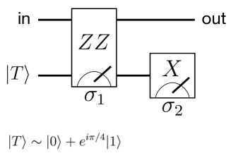
Figure 4: Implementation of the $T$-gate.

The final measurement of $n$ qubits in the $0,1$ basis is equivalent to a non-destructive eigenvalue measurement of $Z_{1},\ldots,Z_{n}$ after which the final state is discarded. This allows one to commute all Clifford gates of $U^{\prime}$ towards the end of the circuit by properly updating which Pauli operator one has to be measured at each step. Once a Clifford gate reaches the end of the circuit, it serves no purpose and can be discarded. We conclude that $U$ can be simulated by a PBC^∗ on $n+m$ qubits. Let $P_{1},\ldots,P_{r}\in{\mathcal{P}}^{n+m}$ be the Pauli operators that have to be measured. We can assume that all Pauli operators $P_{1},\ldots,P_{r}$ pairwise commute. Indeed, suppose this is not the case and let $t$ be the first time step when $P_{t}$ anti-commutes with $P_{s}$ for some $s<t$. Let $\phi$ be the state reached just before the measurement of $P_{t}$. Note that $P_{s}\phi=\pm\phi$ and thus $(I+\sigma_{t}P_{t})\phi=(\sigma_{t}P_{t}\pm P_{s})\phi$. One can easily check that an operator $V\equiv(\sigma_{t}P_{t}\pm P_{s})/\sqrt{2}$ is a Clifford unitary operator whenever $P_{t}$ and $P_{s}$ anticommute. This shows that both outcomes $\sigma_{t}$ have the same probability and the measurement of $P_{t}$ has the same effect as drawing $\sigma_{t}$ from the uniform distribution and applying the Clifford unitary $V$ defined above. Such a unitary $V$ can be commuted towards the end of the circuit and discarded. Hence we can assume that all operators $P_{1},\ldots,P_{r}$ pairwise commute. Furthermore, one can append the sequence $P_{1},\ldots,P_{r}$ at the beginning with dummy Pauli measurements of $Z_{i}$ for all qubits $i$ initialized in the $|0\rangle$ state. Applying the above argument again one can modify the sequence $P_{1},\ldots,P_{r}$ such that all $P_{t}$ commute with the dummy measurements, that is, any operator $P_{t}$ acts trivially on the qubits initialized in the $|0\rangle$ state. Therefore such qubits serve no purpose and can be discarded. We have shown that the original circuit $U$ can be simulated by a PBC on $m$ qubits with $r$ steps and pairwise commuting Pauli operators $P_{1},\ldots,P_{r}$. Furthermore, since the number of independent pairwise commuting Pauli operators on $m$ qubits is at most $m$, we can assume that $r\leq m$, that is, the PBC has the standard form. This completes the proof of Theorem 2.

Let us now prove Theorem 3. Let ${\mathcal{Q}}$ be a fixed PBC on $n+k$ qubits and let $p({\mathcal{Q}})$ be the probability that the final outcome of ${\mathcal{Q}}$ is $b_{out}=1$. Our goal is to approximate $p({\mathcal{Q}})$ on a classical computer assisted by a PBC on $n$ qubits. Suppose one can find a decomposition

$$|H\rangle\langle H|^{\otimes k}=\sum_{i=1}^{\chi}\alpha_{i}|\phi_{i}\rangle\langle\phi_{i}|$$ (12)

for some $k$-qubit stabilizer states $\phi_{i}$ and some real coefficients $\alpha_{i}$. By linearity, one has

$$p({\mathcal{Q}})=\sum_{i=1}^{\chi}\alpha_{i}p({\mathcal{Q}}_{i}),$$ (13)

where ${\mathcal{Q}}_{i}$ is a PBC-type computation obtained from ${\mathcal{Q}}$ by initializing the first $k$ qubits in the state $\phi_{i}$ rather than $|H\rangle^{\otimes k}$. We note that any stabilizer state $\phi_{i}$ can be represented as $|\phi_{i}\rangle=U_{i}|0\rangle^{\otimes k}$ for some Clifford unitary $U_{i}$. Commuting $U_{i}$ towards the end of ${\mathcal{Q}}_{i}$ and properly updating which Pauli operator has to be measured at each step we can assume that $|\phi_{i}\rangle=|0\rangle^{\otimes k}$ for all $i$. As we have already showed above, such computation ${\mathcal{Q}}_{i}$ is equivalent to a PBC on $n$ qubits. Let $b_{i}$ be the output bit of ${\mathcal{Q}}_{i}$ such that $\mathbb{E}(b_{i})=p({\mathcal{Q}}_{i})$. Define a random variable

$$\xi=\sum_{i=1}^{\chi}\alpha_{i}b_{i}.$$

The above shows that $\xi$ is an unbiased estimator of $p({\mathcal{Q}})$ and one can generate a sample of $\xi$ by repeating a PBC on $n$ qubits $\chi$ times. Since all variables $b_{i}$ are independent, the variance of $\xi$ is bounded as

$$\sigma^{2}\equiv\mathbb{E}(\xi^{2})-\mathbb{E}(\xi)^{2}\leq\sum_{i=1}^{\chi}\alpha_{i}^{2}.$$ (14)

Using the Monte Carlo method one can estimate $p({\mathcal{Q}})$ with a constant precision by generating $M=\min{\{1,O(\sigma^{2})\}}$ independent samples of $\xi$. Thus the overall cost of adding $k$ virtual qubits is

$$C\sim\chi\max{\left(1,\sum_{i=1}^{\chi}\alpha_{i}^{2}\right)}.$$

It remains to choose a decomposition in Eq. (12). One can decompose each copy of $|H\rangle\langle H|$ as a linear combination of stabilizer states using the identity

$$|H\rangle\langle H|=\alpha_{1}|0\rangle\langle 0|+\alpha_{2}|1\rangle\langle 1|+\alpha_{3}|+\rangle\langle+|,$$ (15)

where

$$\alpha_{1}=\frac{1}{2},\quad\alpha_{2}=\frac{1-\sqrt{2}}{2},\quad\alpha_{3}=\frac{1}{\sqrt{2}}$$

and then take the tensor product decomposition. Thus $\chi=3^{k}$ and $C\sim\chi=2^{O(k)}$. This completes the proof of Theorem 3.

Appendix A

In this section we prove Lemma 2. Since the constant term $f_{\emptyset}$ contributes a multiplicative factor $\omega^{m}$ to $\langle f\rangle$, we can assume wlog that $f_{\emptyset}=0$. Define coefficients $g_{1},\ldots,g_{n}\in\mathbb{Z}_{2}$ such that

$$g_{a}=\left\{\begin{array}[]{rcl}0&\mbox{if}&f_{a}=1{\pmod{4}},\\ 1&\mbox{if}&f_{a}=3{\pmod{4}},\\ f_{a}/2&\mbox{if}&f_{a}=0,2{\pmod{4}}.\\ \end{array}\right.$$

Let $S\subseteq[n]$ be the set of indexes $a$ such that $f_{a}=1,3{\pmod{4}}$. A simple algebra shows that

$$\omega^{f(x)}=i^{\sum_{a\in S}x_{a}}\cdot(-1)^{g(x)},$$

where

$$g(x)=\sum_{a=1}^{n}g_{a}x_{a}+\sum_{1\leq a<b\leq n}f_{a,b}x_{a}x_{b}.$$

Let us first assume that $S\neq\emptyset$. Without loss of generality $S\ni n$ (otherwise permute the variables). Define a new summation variable $y\in\mathbb{F}_{2}^{n}$ such that $y_{a}=x_{a}$ for $a=1,\ldots,n-1$ and $y_{n}=\sum_{a\in S}x_{a}$. Note that

$$x_{a}=\left\{\begin{array}[]{rcl}y_{a}&\mbox{if}&a=1,\ldots,n-1,\\ y_{n}+\sum_{a\in S\backslash n}y_{a}&\mbox{if}&a=n.\\ \end{array}\right.$$

Using the identity

$$i^{\sum_{a\in S}x_{a}}=i^{\sum_{a\in S}x_{a}{\pmod{2}}}\cdot(-1)^{\sum_{a<b\in S}x_{a}x_{b}}$$

one arrives at

$$\langle f\rangle=\sum_{y\in\mathbb{F}_{2}^{n}}i^{y_{n}}\cdot(-1)^{h(y)}$$

with

$$h(y) = \sum_{a\notin S}g_{a}y_{a}+\sum_{a\in S\backslash n}(g_{a}+g_{n})y_{a}+g_{n}y_{n}$$

$$+\sum_{1\leq a<b\leq n-1}f_{a,b}y_{a}y_{b}+\sum_{a=1}^{n-1}f_{a,n}y_{a}y_{n}$$

$$+\sum_{a=1}^{n-1}\sum_{b\in S\backslash n}f_{a,n}y_{a}y_{b}.$$

Let us split the sum over $y$ into two terms corresponding to $y_{n}=0,1$. We get

$$\langle f\rangle=S_{0}+iS_{1},$$

where

$$S_{\epsilon}=\sum_{z\in\mathbb{F}_{2}^{n-1}}(-1)^{h(z,\epsilon)},\quad\quad\epsilon=0,1.$$

Using the definition of $h(y)$ one gets

$$h(z,\epsilon)=\sum_{1\leq a<b\leq n-1}H_{a,b}z_{a}z_{b}+L_{\epsilon}(z)$$

where $L_{\epsilon}(z)$ is a linear Boolean function and $H$ is a symmetric binary matrix with zero diagonal. Importantly, the matrix $H$ does not depend on $\epsilon$. It is well-known that any matrix $H$ as above can be transformed into a block-diagonal form with all non-zero blocks being $\left[\begin{array}[]{cc}0&1\\ 1&0\\ \end{array}\right]$ by a transformation $H\to V^{T}HV$, where $V$ is an invertible binary matrix MacWilliams and Sloane (1977). The number of non-zero blocks in $V^{T}HV$ is $r$, where $2r$ is the rank of $H$ (which is always even). Moreover, the matrix $V$ can be computed in time $O(n^{3})$ using the standard linear algebra methods MacWilliams and Sloane (1977). Performing a change of variable $z\to Vz$ and defining new linear functions $L^{\prime}_{\epsilon}(z)=L_{\epsilon}(Vz)$ one gets

$$S_{\epsilon}=\sum_{z\in\mathbb{F}_{2}^{n-1}}(-1)^{\sum_{a=1}^{r}z_{2a-1}z_{2a}+L^{\prime}_{\epsilon}(z)}.$$

Obviously, $S_{\epsilon}=0$ if $L^{\prime}_{\epsilon}(z)$ includes at least one of the variables $z_{a}$ with $2r<a\leq n-1$. Otherwise one gets

$$S_{\epsilon}=2^{n-1-2r}\prod_{a=1}^{r}S_{\epsilon,a},$$

where

$$S_{\epsilon,a}=\sum_{z_{2a-1},z_{2a}=0,1}(-1)^{z_{2a-1}z_{2a}+u(\epsilon,a)z_{2a-1}+v(\epsilon,a)z_{2a}}$$

for some coefficients $u(\epsilon,a)=0,1$ and $v(\epsilon,a)=0,1$ determined by $L^{\prime}_{\epsilon}$. A direct inspection shows that $S_{\epsilon,a}$ takes values $0$ and $\pm 2$. We conclude that $S_{\epsilon}$ takes values $0$ and $\pm 2^{n-1-r}$. This leaves only nine possible combinations for $\langle f\rangle=S_{0}+iS_{1}$, Namely, $\langle f\rangle=0$ (if both $S_{0}$ and $S_{1}$ are zero), or $\langle f\rangle=2^{n-1-r}\omega^{2m}$ for some $m\in\mathbb{Z}_{4}$ (if exactly one of $S_{0}$ and $S_{1}$ is non-zero), or $\langle f\rangle=2^{n-1-r+1/2}\omega^{2m+1}$ for some $m\in\mathbb{Z}_{4}$ (if both $S_{0}$ and $S_{1}$ are non-zero). This is equivalent to the statement of Lemma 2. The case when $S=\emptyset$ is completely analogous.

Appendix B

In this section we describe a numerical method for computing a low-rank decomposition of a given target state $\phi$ into stabilizer states. We shall be mostly interested in the case $|\phi\rangle=|H^{\otimes n}\rangle$.

Let $\mathcal{S}_{n}$ be the set of pure $n$-qubit stabilizer states. Given a target $n$-qubit state $\phi$ and an integer $\chi$ we would like to check whether $\phi$ admits a decomposition

$$|\phi\rangle=\sum_{a=1}^{\chi}c_{a}|\phi_{a}\rangle$$ (16)

for some $\phi_{1},\ldots,\phi_{\chi}\in\mathcal{S}_{n}$. It is known Aaronson and Gottesman (2004) that the size of $\mathcal{S}_{n}$ grows asymptotically as $2^{(1/2+o(1))n^{2}}$. Thus performing an exhaustive search over all $\chi$-tuples of $n$-qubit stabilizer states becomes impractical even for small values of $n$. Instead, we used a Monte Carlo algorithm that performs a random walk on the set of $\chi$-tuples $(\phi_{1},\ldots,\phi_{\chi})\in\mathcal{S}_{n}^{\chi}$ and tries to maximize a suitable objective function $F(\phi_{1},\ldots,\phi_{\chi})$. Specifically, we choose $F(\phi_{1},\ldots,\phi_{\chi})=\|\Pi\phi\|$, where $\Pi$ is the projector onto the linear subspace spanned by $\phi_{1},\ldots,\phi_{\chi}$. Assuming that $\|\phi\|=1$, the decomposition Eq. (16) is possible iff $\max F(\phi_{1},\ldots,\phi_{\chi})=1$.

We define the random walk on $\mathcal{S}_{n}^{\chi}$ using the Glauber dynamics. Let $\beta>0$ be some fixed parameter which has a meaning of the inverse temperature. At each step of the walk we randomly choose a state label $a\in\{1,2,\ldots,\chi\}$ and a Pauli operator $P\in\mathcal{P}^{n}$. All choices are made with respect to the uniform distribution. We perform a tentative move $\phi_{a}\to\phi_{a}^{\prime}=c(I+P)\phi_{a}$, where $c$ is a normalizing coefficient. One can easily check that this move maps stabilizer states to stabilizer states. If the move increases the value of the objective function $F$, we accept the new state $\phi_{a}^{\prime}$, that is, $\phi_{a}$ is replaced by $\phi_{a}^{\prime}$. Otherwise, the new state $\phi_{a}^{\prime}$ is accepted with a probability $p_{acc}=\exp{[-\beta(F-F^{\prime})]}$, where $F$ and $F^{\prime}$ are the values of the objective function before and after the move. If $(I+P)\phi_{a}=0$, the move is rejected right away. The walk is stopped as long as we observe a tuple of states with $F=1$. We start with relatively small values $\beta=\beta_{in}$ and gradually increase $\beta$ using the geometric sequence until it reaches the final value $\beta=\beta_{f}$. This corresponds to the simulated annealing method. For each value of $\beta$ the random walk was repeated for $M\gg 1$ steps. In practice we used values $\beta_{in}=1$, $\beta_{f}=4000$, and $M=1000$. The number of annealing steps was chosen as $100$. Since we worked with relatively small values of $n$, the stabilizer states $\phi_{j}$ were represented by vectors of size $2^{n}$.

Since our target state $|\phi\rangle=|H^{\otimes n}\rangle$ has real amplitudes in the computational basis, one can easily show that the optimal decomposition Eq. (16) can be chosen such that all stabilizer states $\phi_{a}$ have real amplitudes as well (the real part of a stabilizer state is either zero or proportional to a stabilizer state). Accordingly, we restricted the random walk to the subset of $\mathcal{S}_{n}^{\chi}$ corresponding to real stabilizer states. Clearly, a move $\phi_{j}\to\phi_{j}^{\prime}=c(I+P)\phi_{j}$ maps real states to real states if $P$ contains even number of $Y$’s. The move was accepted only if this condition is satisfied.

The best decompositions of $|H^{\otimes n}\rangle$ found using this method are shown below. Here we use the notations of Section IV, so that $|H\rangle=|0\rangle+(\sqrt{2}-1)|1\rangle$.

$$|H^{\otimes 2}\rangle=(2-\sqrt{2})|E_{2}\rangle+(-1+\sqrt{2})|K_{2}\rangle.$$

$$|H^{\otimes 3}\rangle=(-8+6\sqrt{2})|B_{3,3}\rangle+(2-\sqrt{2})|E_{3}\rangle+(-1+\sqrt{2})|K_{3}\rangle.$$

$$|H^{\otimes 4}\rangle=(4-2\sqrt{2})|B_{4,0}\rangle+(20-14\sqrt{2})|B_{4,4}\rangle+(-4+3\sqrt{2})|O_{4}\rangle+(-3+2\sqrt{2})Z^{\otimes 4}|K_{4}\rangle.$$

$$|H^{\otimes 5}\rangle = (-16+12\sqrt{2})|B_{5,0}\rangle+(-40+28\sqrt{2})|B_{5,5}\rangle+(-4+3\sqrt{2})|O_{5}\rangle+(10-7\sqrt{2})|E_{5}\rangle$$

$$+(3-2\sqrt{2})K|O_{5}\rangle+(7-5\sqrt{2})K|E_{5}\rangle.$$

Here $K=\prod_{i<j}\Lambda(Z)_{i,j}$ applies cnotrolled-Z to each pair of qubits. The stabilizer decomposition of $|H^{\otimes 6}\rangle$ is shown in Eq. (11). By definition, the number of terms $\chi$ in these decompositions gives an upper bound on the stabilizer rank $\chi_{n}$. We conjecture that all above decompositions and the one in Eq. (11) are optimal in the sense that $\chi=\chi_{n}$.

Appendix C

Let $\chi_{n}$ be the stabilizer rank of $|H^{\otimes n}\rangle$. Here we prove a lower bound $\chi_{n}=\Omega(n^{1/2})$.

Let $\phi$ be a pure $n$-qubit state. Define the $T$-count of $\phi$ denoted $\tau(\phi)$ as the minimum integer $\tau$ such that $\phi$ can be prepared starting from the all-zeros state by a quantum circuit composed of Clifford gates, $T$-gates, and (postselective) eigenvalue measurements of Pauli operators, such that the number of $T$-gates is at most $\tau$. We claim that

$$\chi_{\tau(\phi)}\geq\chi(\phi).$$ (17)

Indeed, as was shown in Section V, the $T$-gate can be realized by a gadget that consumes one copy of the magic state $|H\rangle$ and performs (postselective) Pauli measurements. Thus we can prepare $\phi$ starting from $\tau(\phi)$ copies of the magic state $|H\rangle$ by a sequence of (postselective) Pauli measurement and Clifford operations. Since the latter do not increase stabilizer rank, we can write $\phi$ as a linear combination of $\chi_{\tau(\phi)}$ stabilizer states. This is equivalent to Eq. (17).

We shall now choose a state $\phi$ will a relatively small $T$-count and a large stabilizer rank. Define

$$|\phi_{n}\rangle=|\theta_{1}\otimes\theta_{2}\otimes\cdots\otimes\theta_{n}\rangle,\quad\quad|\theta_{k}\rangle=|0\rangle+(2^{k+1}-1)|1\rangle.$$

Lemma 4.

The state $\phi_{n}$ has $2^{n}$ distinct amplitudes in the computational basis.

We postpone the proof of the lemma until the end of the section. Let us first show that $\phi_{n}$ has a large stabilizer rank. Indeed, any stabilizer state has $C=O(1)$ distinct amplitudes in the computational basis. Thus any linear combination of $\chi$ stabilizer states has at most $C^{\chi}$ distinct amplitudes. Applying this to $\phi_{n}$ one gets $C^{\chi(\phi_{n})}\geq 2^{n}$, that is, $\chi(\phi_{n})=\Omega(n)$.

Let us now show that $\phi_{n}$ has a small $T$-count. First we claim that the state $\theta_{k}$ has $T$-count $O(k)$. Indeed, we can first prepare a state $|+\rangle^{\otimes(k+1)}\otimes|0\rangle$ and then apply multiple control CNOT gate $\Lambda^{k+1}(X)$ such that the last qubit is the target one. This creates a state

$$\sum_{x\in\{0,1\}^{k+1}}|x_{1},x_{2},\ldots,x_{k+1}\rangle\otimes|x_{1}x_{2}\cdots x_{k+1}\rangle.$$

Measuring the first $k+1$ qubits in the $X$-basis and postselecting the outcome $+$ leaves the last qubit in a state $(2^{k+1}-1)|0\rangle+|1\rangle$, which coincides with $\theta_{k}$ modulo a bit-flip. One can easily check that the multiple control CNOT gate $\Lambda^{k+1}(X)$ can be implemented using $O(k)$ Toffoli gates. Furthermore, the Toffoli gate can be implemented using seven $T$-gates Amy et al. (2013); Gosset et al. (2014). Thus $\theta_{k}$ has $T$-count $O(k)$ and therefore $\phi_{n}$ has $T$-count $O(\sum_{k=1}^{n}k)=O(n^{2})$. Substituting this into Eq. (17) yields $\chi_{n^{2}}\geq\Omega(n)$, that is, $\chi_{n}=\Omega(n^{1/2})$.

Proof of Lemma 4.

Consider any basis vector $x\in\mathbb{F}_{2}^{n}$. Let $K\subseteq\{1,2,\ldots,n\}$ be the support of $x$. Then

$$\langle x|\phi_{n}\rangle=\prod_{k\in K}(2^{k+1}-1).$$

The lemma follows from the following fact.

Proposition 1.

Suppose $K,M\subseteq[2,\infty)$ are finite subsets of integers such that

$$\prod_{k\in K}(2^{k}-1)=\prod_{m\in M}(2^{m}-1).$$ (18)

Then $K=M$.

Proof.

First we claim that

$$\prod_{b\geq a}(1-2^{-b})>1-2^{-a+1}\quad\mbox{for all $a\geq 1$}.$$ (19)

Indeed, define $x=2^{-a}$. Then

$$\prod_{b\geq a}(1-2^{-b})^{-1}=\prod_{b\geq 0}(1-x2^{-b})^{-1}$$

$$=1+\sum_{p=1}^{\infty}x^{p}\prod_{q=1}^{p}(1-2^{-q})^{-1}.$$

Define $\xi_{p}=\prod_{q=1}^{p}(1-2^{-q})$. One can easily check that $\xi_{p}>\lim_{p\to\infty}\xi_{p}>1/4$. Since $\xi_{1}=1/2$, one gets

$$\prod_{b\geq a}(1-2^{-b})^{-1}<1+2x+4\sum_{p=2}^{\infty}x^{p}\leq\sum_{p=0}^{\infty}(2x)^{p}=(1-2x)^{-1}.$$

This is equivalent to Eq. (19).

Now let $s(K)$ and $s(M)$ be the sum of all elements in $K$ and $M$ respectively. Assume wlog that $s(K)\geq s(M)$. Then Eq. (18) implies

$$2^{s(K)-s(M)}=\frac{\prod_{m\in M}(1-2^{-m})}{\prod_{k\in K}(1-2^{-k})}$$

$$\leq\frac{1}{\prod_{k\geq 2}(1-2^{-k})}<\frac{1}{1-2^{-1}}=2.$$

Here the last inequality follows from Eq. (19). Thus $s(K)=s(M)$ and

$$\prod_{k\in K}(1-2^{-k})=\prod_{m\in M}(1-2^{-m})\equiv\xi.$$ (20)

Let $k_{1}$ and $m_{1}$ be the smallest elements of $K$ and $M$ respectively. Assume wlog that $m_{1}\geq k_{1}$. Let us show that in fact $m_{1}=k_{1}$. Indeed, otherwise $m_{1}\geq k_{1}+1$. Then Eq. (20) implies $\xi\leq 1-2^{-k_{1}}$ and

$$\xi\geq(1-2^{-m_{1}})\prod_{b\geq m_{1}+1}(1-2^{-b})>(1-2^{-m_{1}})^{2}.$$

Here the last inequality follows from Eq. (19). Thus $(1-2^{-m_{1}})^{2}<1-2^{-k_{1}}$ which implies $m_{1}<k_{1}+1$ leading to a contradiction. We conclude that $k_{1}=m_{1}$. Thus we can cancel the factor $(1-2^{-k_{1}})$ in both parts of Eq. (20) and use induction in the number of elements in the largest of the sets $K,M$ to show that $K=M$. ∎

∎

Finally, let us sketch an argument that could potentially provide a stronger lower bound on $\chi_{n}$. Consider a decomposition $|H^{\otimes n}\rangle=\sum_{\alpha=1}^{\chi}c_{\alpha}|\phi_{\alpha}\rangle$, where $\phi_{\alpha}$ are normalized stabilizer states. We can assume wlog that $\phi_{\alpha}$ are linearly independent. Define a vector $c=(c_{1},\ldots,c_{\chi})$ and a Gram matrix $G_{\alpha,\beta}=\langle\phi_{\alpha}|\phi_{\beta}\rangle$. Then $\langle c|G|c\rangle=1$. Let $g_{min}>0$ be the smallest eigenvalue of $G$. Then $G\geq g_{min}I$ and thus $\|c\|^{2}\leq g_{min}^{-1}$. Let $\delta_{n}$ be the largest magnitude of the overlap between $|H^{\otimes n}\rangle$ and a normalized $n$-qubit stabilizer state. One can easily check that $\delta_{n}\leq 2^{-\Omega(n)}$. The identity $1=\sum_{\alpha=1}^{\chi}c_{\alpha}^{*}\langle\phi_{\alpha}|H^{\otimes n}\rangle$ implies $1\leq\delta_{n}\|c\|_{1}\leq\chi^{1/2}\delta_{n}\|c\|$. We conclude that $\chi\geq g_{min}\delta_{n}^{-2}\geq g_{min}2^{\Omega(n)}$. This proves that $\chi\geq 2^{\Omega(n)}$ in the special case when all states $\phi_{\alpha}$ are pairwise orthogonal, that is, $g_{min}=1$.

References

- Shor (1994) P. W. Shor, Proceedings of the 35th Annual Symposium on Foundations of Computer Science pp. 124–134 (1994).
- Hallgren (2007) S. Hallgren, Journal of the ACM (JACM) 54, 4 (2007).
- Lloyd (1996) S. Lloyd, Science 273, 1073 (1996).
- Raussendorf and Briegel (2001) R. Raussendorf and H. J. Briegel, Phys. Rev. Lett. 86, 5188 (2001).
- Aharonov et al. (2007) D. Aharonov, W. Van Dam, J. Kempe, Z. Landau, S. Lloyd, and O. Regev, SIAM J. of Computing 37, 166 (2007).
- Knill and Laflamme (1998) E. Knill and R. Laflamme, Phys. Rev. Lett. 81, 5672 (1998).
- Cleve and Watrous (2000) R. Cleve and J. Watrous, Proceedings of the 41st Annual Symposium on Foundations of Computer Science pp. 526–536 (2000).
- Terhal and DiVincenzo (2004) B. Terhal and D. DiVincenzo, Quant. Inf. Comp. 4, 134 (2004).
- Shepherd and Bremner (2009) D. Shepherd and M. Bremner, Proc. R. Soc. A 465, 1413 (2009).
- Gottesman (1998) D. Gottesman, Phys. Rev. A 57, 127 (1998).
- Steane (1997) A. M. Steane, Phys. Rev. Lett. 78, 2252 (1997).
- Fowler et al. (2009) A. Fowler, A. Stephens, and P. Groszkowski, Phys. Rev. A 80, 052312 (2009).
- Bravyi and Kitaev (2005) S. Bravyi and A. Kitaev, Phys. Rev. A 71, 022316 (2005).
- Meier et al. (2012) A. Meier, B. Eastin, and E. Knill, arXiv:1204.4221 (2012).
- Bravyi and Haah (2012) S. Bravyi and J. Haah, Phys. Rev. A 86, 052329 (2012).
- Jones (2013) C. Jones, Phys. Rev. A 87, 042305 (2013).
- Fowler et al. (2013) A. Fowler, S. Devitt, and C. Jones, Scientific reports 3, 1939 (2013).
- Campbell and Browne (2009) E. Campbell and D. Browne, arXiv:0908.0838 (2009).
- Aaronson and Gottesman (2004) S. Aaronson and D. Gottesman, Phys. Rev. A 70, 052328 (2004).
- Garcia et al. (2012) H. Garcia, I. Markov, and A. Cross, arXiv preprint arXiv:1210.6646 (2012).
- García et al. (2014) H. J. García, I. Markov, and A. Cross, Quant. Inf. and Comp. 14, 683 (2014).
- Strassen (1969) V. Strassen, Numerische Mathematik 13, 354 (1969).
- Coppersmith and Winograd (1987) D. Coppersmith and S. Winograd, Proceedings of the 19th Annual Symposium on Foundations of Computer Science pp. 1–6 (1987).
- Chitambar et al. (2008) E. Chitambar, R. Duan, and Y. Shi, Phys. Rev. Lett. 101, 140502 (2008).
- Veitch et al. (2012) V. Veitch, C. Ferrie, D. Gross, and J. Emerson, New J. Phys. 14, 113011 (2012).
- Howard et al. (2014) M. Howard, J. Wallman, V. Veitch, and J. Emerson, Nature 510, 351 (2014).
- Pashayan et al. (2015) H. Pashayan, J. Wallman, and S. Bartlett, arXiv preprint arXiv:1503.07525 (2015).
- Delfosse et al. (2014) N. Delfosse, P. Guerin, J. Bian, and R. Raussendorf, arXiv preprint arXiv:1409.5170 (2014).
- Markov and Shi (2008) I. Markov and Y. Shi, SIAM J. on Comp. 38, 963 (2008).
- Dehaene and De Moor (2003) J. Dehaene and B. De Moor, Phys. Rev. A 68, 042318 (2003).
- Van den Nest (2010) M. Van den Nest, Quant. Inf. Comp. 10, 0258 (2010).
- MacWilliams and Sloane (1977) F. MacWilliams and N. Sloane, The theory of error correcting codes (Elsevier, 1977).
- Amy et al. (2013) M. Amy, D. Maslov, M. Mosca, and M. Roetteler, Computer-Aided Design of Integrated Circuits and Systems, IEEE Transactions on 32, 818 (2013).
- Gosset et al. (2014) D. Gosset, V. Kliuchnikov, M. Mosca, and V. Russo, Quant. Inf. and Comp. 14, 1261 (2014).