Modal locking between vocal fold and vocal tract oscillations: Simulations in time domain

Abstract

During voiced speech, the human vocal folds interact with the vocal tract acoustics. The resulting glottal source-resonator coupling has been observed using mathematical and physical models as well as in in vivo phonation. We propose a computational time-domain model of the full speech apparatus that, in particular, contains a feedback mechanism from the vocal tract acoustics to the vocal fold oscillations. It is based on numerical solution of ordinary and partial differential equations defined on vocal tract geometries that have been obtained by Magnetic Resonance Imaging. The model is used to simulate rising and falling pitch glides of [, i] in the fundamental frequency ($f_{o}$) interval $[150\,\mathrm{Hz},320\,\mathrm{Hz}]$. The interval contains the first vocal tract resonance $f_{R1}$ and the first formant $F_{1}$ of [i] as well as the fractions of the first resonance $f_{R1}/4$ and $f_{R1}/3$ of [].

The simulations reveal a locking pattern of the $f_{o}$-trajectory at $f_{R1}$ of [i] in falling and rising glides. The resonance fractions of [] produce perturbations in the pressure signal at the lips but no locking. All these observations from the model behaviour are consistent and robust within a wide range of feasible model parameter values and under exclusion of secondary model components.

Index Terms: Speech modelling, vocal fold model, flow induced vibrations, modal locking.

1 Introduction

The classical source–filter theory of vowel production is built on the assumption that the source (i.e., the vocal fold vibration) operates independently of the filter (i.e., the vocal tract, henceforth VT) whose resonances modulate the resulting vowel sound [1, 2]. Even though this approach captures a wide range of phenomena in speech production, at least in male speakers, some observations remain unexplained by the source–filter model lacking feedback. The purpose of this article is to deal with some of these observations using computational modelling.

More precisely, simulated rising and falling frequency glides of vowels [] and [i] over the frequency range $[150\,\mathrm{Hz},320\,\mathrm{Hz}]$ are considered. Similar glides recorded from eleven female test subjects are treated in the companion article [3]. Such a vowel glide is particularly interesting if its glottal frequency ($f_{o}$) range intersects an isolated acoustic resonance of the supra- or subglottal cavity, which we here assume to correspond to the lowest formant $F_{1}$. Since $F_{1}$ almost always lies high above $f_{o}$ in adult male phonation, this situation occurs typically in female subjects and only when they are producing vowels such as [i] with low $F_{1}$. As reported below, simulations reveal (in addition to other observations) a characteristic locking behaviour of $f_{o}$ at the VT acoustic resonance $f_{R1}\approx F_{1}$. To check the robustness of the model observations, secondary features of the model and the role of unmodelled physics are discussed at the end of the article.

As a matter of fact, this article has two equally important objectives. Firstly, we pursue better understanding of the time-domain dynamics of glottal pulse perturbations near $f_{R1}$ of [i] and at other acoustic “hot spots” of the VT and the subglottal system within $[150\,\mathrm{Hz},320\,\mathrm{Hz}]$ that may be reached in speech or singing. An acoustic and flow-mechanical model of the speech apparatus is a well-suited tool for this purpose. Secondly, we introduce and validate a computational model that meets these requirements. The proposed model has been originally designed to be a glottal pulse source for high-resolution 3D computational acoustics model of the VT which is being developed for medical purposes [5]. There is an emerging application for this model as a development platform of speech signal processing algorithms such as discussed in [6], [7] and [8]; however, the model introduced in [9] has been used in [8]. Since perturbations of $f_{o}$ near $F_{1}$ are a widely researched, yet quite multifaceted phenomenon, it is a good candidate for model validation experiments.

The simulations carried out in this paper indicate special kinds of perturbations in vocal folds vibrations near a VT resonance as reported below. The mere existence of such perturbations is not surprising considering the wide range of existing literature. Since the seminal work of [10], a wide range of glottal source perturbation patterns related to acoustic loading has been investigated. Experiments were carried out in [11] on excised larynges mounted on a resonator to determine how glottal amplitude ratio changes with the subglottal resonator length. Physical models were used in [12] with a subglottal resonator to study phonation onsets and offsets, and in [13] with sub- and supraglottal resonators to study phonation onsets. The latter also considered the dynamics of frequency jumps as the natural frequency of their physical model was varied over time. Similarly, a physical model of phonation with tubular, variable length supraglottal resonator was studied in [14, 15], and it was used to validate a flow-acoustic model somewhat resembling the one proposed in this article.

In [16] the problem was approached using both reasoning based on sub- and supraglottal impedances and a non-computational flow model as well as computational model comprising a multi-mass vocal fold model and wave-reflection models of the subglottal and supraglottal systems. A two-mass model of vocal folds, coupled with a variable-length resonator tube, was used in [17], and pitch glides were simulated using a four-mass model to analyse the interactions between vocal register transitions and VT resonances in [18].

These works reveal a consistent picture of the existence of perturbations caused by resonant loads, and this phenomenon has also been detected experimentally in [19] using speech recordings and in [20] using simultaneous recordings of laryngeal endoscopy, acoustics, aerodynamics, electroglottography, and acceleration sensors. The latter article also contains a review on related voice bifurcations.

Although the existence of these perturbations has been well reported, speech modelling studies have given only limited attention to the time-domain dynamics of fundamental frequency glides where such perturbations would be expected to occur. Of the above mentioned studies, upward glides were simulated in [13] by varying the natural frequency of their physical model over time. Their small amplitude oscillation model exhibited a frequency jump in the vicinity of the resonance of their downstream tube when the load resistance was sufficiently strong. Downward glides were simulated in [16] followed by upward glides by varying the parameters of a multi-mass vocal fold model. Frequency jumps, subharmonics and amplitude changes were observed in the regions where load reactances were changing rapidly. Changes in the rate of change of the fundamental frequency in these regions can also be seen in their Figures 10-14. In [18] upward glides were simulated followed by downward glides by adjusting the tension parameter (i.e. decreasing masses and increasing stiffness parameters by the same factor) in their four-mass vocal fold model. They observed frequency jumps associated with register changes, which in turn were shown to occur at different frequencies depending on the vocal tract load.

Some of the most popular approaches to modelling phonation are based on the Kelly–Lochbaum vocal tract [21] or various transmission line analogues [22, 23, 24]. Contrary to these approaches, the proposed model consists of (ordinary and partial) differential equations, conservation laws, and coupling equations. In this modelling paradigm, the temporal and spatial discretisation is conceptually and practically separated from the actual mathematical model of speech. The computational model is simply a numerical solver for the model equations, written in MATLAB environment. The modular design makes it easy to decouple model components for assessing their significance to simulated behaviour. Since the generalised Webster’s equation for the VT acoustics assumes intersectional area functions as its geometric data, VT configurations from Magnetic Resonance Imaging (MRI) can be used without transcription to non-geometric model parameters. Thus, time-dependent VT geometries are easy to implement. Further advantages of speech modelling based on Webster’s equation have been explained in [26] where the approach is somewhat similar to one taken here.

The proposed model aims at qualitatively realistic functionality, tunability by a low number of parameters, and tractability of model components, equations, and their relation to biophysics. Similar functionality in higher precision can be obtained using Computational Fluid Dynamics (CFD) with elastic tissue boundaries. In the CFD approach, the aim is to model the speech apparatus as undivided whole [27], but the computational cost is much higher compared to our model or the models proposed in, e.g., [26] and [28]. The numerical efficiency is a key issue because some parameter values or their feasible ranges (in particular, for hard-to-get physiological parameters) can only be determined by the trial and error method as discussed in Chapter 4 in [29], leading to a high number of required simulations.

2 Model of the Vocal Folds

2.1 Anatomy, physiology, and control of phonation

All voiced speech sounds originate from self-sustained quasi-periodic oscillations of the vocal folds where the closure of the aperture — known as the rima glottidis — between the two string-like vocal folds cuts off the air flow from lungs. This process is called phonation, and the system comprising the vocal folds and the rima glottidis is known as the glottis. A single period of the glottal flow produced by phonation is known as a glottal pulse. A description of structures in human larynx and their function can be found, e.g., in [30] or [31], and we give here only a brief summary.

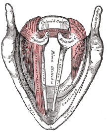
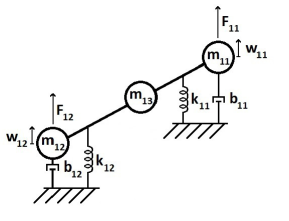
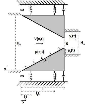
Figure 1: The topmost panel on left: Sketch of the anatomy of the larynx seen from above according to [32]. Right panel: The geometry of the glottis model and the symbols used. The trachea (i.e., the channel leading from the lungs to glottis) is to the left in this sketch and the vocal tract is to the right. The lower panel on left: Lumped-element representation of the glottis model with two degrees of freedom shown for the lower vocal fold ($j=1$).

As shown in Figure 1 (upper left panel), each vocal fold consists of a vocal ligament (also known as a vocal cord) together with a medial part of the thyroarytenoid muscle, and the vocalis muscle (not specified in upper left panel of Figure 1). Left and right vocal folds are attached to the thyroid cartilage from their anterior ends and to the respective left and right arytenoid cartilages from their posterior ends. In addition, there is the fourth, ring-formed cricoid cartilage whose location is inferior to the thyroid cartilage. The vocal folds and the associated muscles are supported by these cartilages.

There are two muscles attached between each of the arytenoid cartilages and the cricoid cartilage: the posterior and the lateral cricoarytenoid muscles whose mechanical actions are opposite. The vocal folds are adducted by the contraction of the lateral cricoarytenoid muscles during phonation, and conversely, abducted by the posterior cricoarytenoid muscles during, e.g., breathing. This control action is realised by a rotational movement of the arytenoid cartilages in a transversal plane. In addition, there is a fifth (unpaired) muscle — the arytenoid muscle — whose contraction brings the arytenoid cartilages closer to each other, thus reducing the opening of the glottis independently of the lateral cricoarytenoid muscles. These rather complicated control mechanisms regulate the type of phonation in the breathy-pressed scale.

The main mechanism controlling the fundamental frequency $f_{o}$ of voiced speech sound is actuated by two cricothyroid muscles (not visible in upper left panel of Figure 1). The contraction of these muscles leads to a rotation of the thyroid cartilage with respect to the cricoid cartilage. As a result, the thyroid cartilage inclines to the anterior direction, thus stretching the vocal folds. The elongation of the string-like vocal folds leads to increased stress which raises the fundamental frequency $f_{o}$ of their longitudinal vibrations. The vertical movement of larynx also rotates cricoid cartilage impacting $f_{o}$. Finally, the phonation and $f_{o}$ are influenced by subglottal pressure through the control of respiratory muscles.

2.2 Glottis model

The anatomic configuration in upper left panel of Figure 1 is idealised as a low-order mass-spring system with aerodynamic surfaces as shown in right panel of Figure 1 and discussed in [33] and [29]. Such lumped-element models have been used frequently (see, e.g., [34], [35], [36], [37], [15], and [38]) since the introduction of the classic two-mass model [10]. For recent reviews of the variety of lumped-element and PDE based models and their applications, see [39], [40] and [41].

The radically simplified glottis model geometry in Figure 1 (right panel) corresponds to the coronal section through the center of the vocal folds. Both the fundamental frequency $f_{o}$ as well as the phonation type can be chosen by adjusting parameter values (see Section 4 in [29]). Register shifts (e.g., from modal register to falsetto) are not in the scope of this model since it would require either modelling the vocal folds as aerodynamically loaded strings or as a high-order mass-spring system that has a string-like “elastic” behaviour.

The vocal fold model in Figure 1 (right panel) consists of two wedge-shaped moving elements that have two degrees of freedom each: each end of the vocal fold can move in the y-direction. Although this causes some distortion to the shape of the wedges, the displacements are small enough that this effect is negligible. The distributed mass of these elements is reduced into three mass points which, for the $j^{\textrm{th}}$ fold, $j=1,2$, are located so that $m_{j1}$ is at $x=L$, $m_{j2}$ at $x=0$, and $m_{j3}$ at $x=L/2$. Here $L$ denotes the thickness of the modelled vocal fold structures. In calculation of the masses, the reduced system retains the mass, and static and inertial moments of a more realistic vocal fold shape (for details, see [33] p. 14). The elastic support of the vocal ligament is approximated by two springs at points $x=l_{1}L$ and $x=l_{2}L$. The equations of motion for the vocal folds are given by

$$\begin{cases}\ M_{1}\ddot{W}_{1}(t)+B_{1}\dot{W}_{1}(t)+K_{1}W_{1}(t)=F_{1}(t),\\ \ M_{2}\ddot{W}_{2}(t)+B_{2}\dot{W}_{2}(t)+K_{2}W_{2}(t)=F_{2}(t),\qquad t\in\mathbb{R},\end{cases}$$ (1)

where $W_{j}=\left[\begin{matrix}w_{j1}&w_{j2}\end{matrix}\right]^{T}$ are the displacements of $m_{j1}$ and $m_{j2}$ in the y-direction as shown in Figure 1 (lower left panel). The loading force pair $F_{j}(t)=\left[\begin{matrix}F_{j1}(t)&F_{j2}(t)\end{matrix}\right]^{T}$ is due to aerodynamic and acoustic pressure forces in Eq. (8) when the glottis is open, and the collision forces in Eq. (4) when the vocal folds are in contact. The respective mass, damping, and stiffness matrices $M_{j}$, $B_{j}$, and $K_{j}$ in (1) are

$$\begin{array}[]{c}M_{j}=\left[\begin{array}[]{cc}m_{j1}+\frac{m_{j3}}{4}&\frac{m_{j3}}{4}\\ \frac{m_{j3}}{4}&m_{j2}+\frac{m_{j3}}{4}\end{array}\right],\hskip 17.07164ptB_{j}=\left[\begin{array}[]{cc}b_{j1}&0\\ 0&b_{j2}\end{array}\right],\vspace{4mm}\\ \textrm{and }\quad K_{j}=\left[\begin{array}[]{cc}l_{1}^{2}k_{j1}+l_{2}^{2}k_{j2}&l_{1}l_{2}(k_{j1}+k_{j2})\\ l_{1}l_{2}(k_{j1}+k_{j2})&l_{2}^{2}k_{j1}+l_{1}^{2}k_{j2}\end{array}\right].\end{array}$$ (2)

The entries of these matrices have been computed by means of Lagrangian mechanics in [33]. The damping matrices $B_{j}$ are diagonal since the dampers are located at the endpoints of the vocal folds. The model supports asymmetric vocal fold vibrations but for this work symmetry is imposed on the vocal folds by using parameters $M=M_{j}$, $K=K_{j}$, and $B=B_{j}$, $j=1,2$, and by setting $F(t)=F_{2}(t)=-F_{1}(t)$. The parameters in equation (2) as well as the loading force components in equation (1) are illustrated in Figure 1 (right and lower left panels).

The glottal openings at the two ends of the vocal folds, denoted by $\Delta W_{i}$, $i=1,2$, are related to equations (1) through

$$\left[\begin{array}[]{c}\Delta W_{1}\\ \Delta W_{2}\end{array}\right]=W_{2}-W_{1}+\left[\begin{array}[]{c}g\\ H_{0}\end{array}\right]$$ (3)

where the rest gap parameters $g$ and $H_{0}$ are as in Figure 1 (right panel). In human anatomy, the parameter $g$ is related to the position and orientation of the arytenoid cartilages.

As is typical in related biomechanical modelling [34, 42, 18], the lumped parameters of the mass-spring system (1)– (2) are in some correspondence to the true masses, material parameters, and geometric characteristics of the sound producing tissues. More precisely, matrices $M$ correspond to the vibrating masses of the vocal folds, including the vocal ligaments together with their covering mucous layers and (at least, partly) the supporting vocalis muscles. The elements of the matrices $K$ are best understood as linear approximations of $k(s)=f/s$ where $f=f(s)$ is the contact force required for deflection $s$ at the center of the string-like vocal ligament in the anatomy shown in Figure 1 (upper left panel). It should be emphasised that the exact numerical correspondence of tissue parameters to lumped model parameters $M$ and $K$ is intractable (and for most practical purposes even irrelevant), and their values in computer simulations must be tuned using measurement data of $f_{o}$ and the measured form of the glottal pulse [29].

2.3 Forces during the closed phase

During the glottal closed phase (i.e., when $\Delta W_{1}(t)<0$ at the narrow end of the vocal folds), there are no proper aerodynamic forces affecting the vocal folds dynamics in equations (1). There are, however, nonlinear spring forces with parameter $k_{H}$, accounting for the elastic collision of the vocal folds. They are accompanied by the resultant acoustic counter pressure from the VT and subglottal cavities, denoted by $p_{c}=p_{c}(t)$ in equation (13) below. Thus, the force pair for equations (1) during glottal closed phase is given by

$$F=F_{H}=\left[\begin{array}[]{c}k_{H}|\Delta W_{1}|^{3/2}-C_{pc}p_{c}\\ C_{pc}p_{c}\end{array}\right]\quad\mathrm{for}\quad\Delta W_{1}<0.$$ (4)

Here, the coupling coefficient $C_{pc}=C_{pc}(t)$ accounts for the moment arms and areas on which $p_{c}$ acts, and it will be given an expression in equation (14).

This approach is related to the Hertz impact model that has been used similarly in [34] and [43]. During the glottal open phase (i.e., when $\Delta W_{1}(t)>0$), the spring force in equations (4) is not enabled. Then the load terms in equation (1) are given by $F(t)=F_{A}(t)$ as introduced below in equation (8) in terms of the aerodynamic forces from the glottal flow.

3 Glottal Flow and the Aerodynamic Force

The air flow within the glottis is assumed to be incompressible and one-dimensional with velocity $V(x,t)$, satisfying the mass conservation law $H(x,t)V(x,t)=H_{1}v_{o}(t)$, where $H(x,t)$ is the height of the flow channel inside the glottis. In the model geometry of Figure 1 (right panel) we have

$$H(x,t)=\Delta W_{2}(t)+\frac{x}{L}(\Delta W_{1}(t)-\Delta W_{2}(t)),\ \ \ x\in[0,L].$$

The velocity $v_{o}(t)$ of the flow through the control area $hH_{1}$ superior to the glottis is described by

$$\dot{v}_{o}(t)=\frac{1}{C_{iner}hH_{1}}\left(p_{sub}-R_{g}(t)v_{o}(t)\right)$$ (5)

where $p_{sub}$ is an ideal pressure source (whose values are given relative to the ambient air pressure) located immediately inferior to the vocal folds, $C_{iner}$ regulates flow inertia, $h$ is the width of the rectangular flow channel, and $R_{g}(t)$ represents the total pressure loss in the glottis. In fact, equation (5) is related to Newton’s second law for the air column in motion. Although the pressure driving phonation originates at the lungs, it is here assumed that physiological mechanisms enable the adequate control of the pressure source $p_{sub}$. Note that due to assumed incompressibility, equation (5) can equivalently be written in terms of position-independent volume flow through the glottis $U(t)=v_{o}(t)hH_{1}$.

To derive equation (5) following [33, Section 2.2], one begins with the pressure loss balance $p_{sub}=p_{g}+p_{a}$ where the $p_{sub}$ is the sum of the glottal pressure loss and the accelerating pressure of the fluid column mass in the airways and lungs. The power of accelerating or decelerating an (incompressible) fluid column is $p_{a}(t)(hH_{1})v_{0}(t)$. This power is equal to the derivative of the kinetic energy of the fluid column, yielding the identity $p_{a}(t)(hH_{1})v_{0}(t)=\rho v_{0}(t)v_{0}^{\prime}(t)(hH_{1})^{2}\int{\frac{d\vec{r}}{A(\vec{r})^{2}}}$ where the integration is extended over the VT and SGT volume. Here $A(\vec{r})$ denotes the area of the fluid column cross-section that contains the position vector $\vec{r}$, and the incompressibility $A(\vec{r})v(\vec{r},t)=hH_{1}v_{0}(t)$ was used. Equation (5) follows from this by denoting $C_{iner}=\rho\int{\frac{d\vec{r}}{A(\vec{r})^{2}}}$. The contribution of the VT to the total inertance can be further integrated to $C_{iner}^{VT}=\rho\int_{0}^{L_{VT}}{\frac{ds}{A(s)}}$ but the inertance of the subglottal masses cannot be expressed similarly in terms of anatomic data. Hence, the parameter $C_{iner}$ has to be used as a tuning parameter.

The total pressure loss in the glottis in equation (5) consists of two components, namely

$$R_{g}(t) =R_{v}(t)+R_{t}(t),\quad\text{ where }$$ (6)

$$R_{v}(t) =\frac{12\mu H_{1}L_{g}}{\Delta W_{1}(t)^{3}}\quad\text{ and }\quad R_{t}(t)=k_{g}\frac{\rho H_{1}^{2}v_{o}(t)}{2\Delta W_{1}(t)^{2}}.$$

The first term $R_{v}(t)$ represents the viscous pressure loss, and it is motivated by the Hagen–Poiseuille law in a narrow aperture. It approximates the pressure loss in the glottis using a rectangular tube of width $h$, height $\Delta W_{1}$, and length $L_{g}$. The parameter $\mu$ is the kinematic viscosity of air. The second term $R_{t}(t)$ takes into account the pressure losses not attributable to viscosity in the sense of $R_{v}$, and its form is motivated by the experimental work in [44]. The coefficient $k_{g}$ represents the difference between energy loss at the glottal inlet and pressure recovery at the outlet. This coefficient depends not only on the glottal geometry but also on the glottal opening, subglottal pressure, and flow through the glottis [45]. It should be noted that equations (5)–(6) bear resemblance to the description of airflow in [14, 15] where the pressure loss and recovery effects, however, are accounted for by flow separation in a diverging channel.

The pressure $p=p(x,t)$ in the glottis is given in terms of $v_{0}$ from equation (5) by making use of the mass conservation and the Bernoulli theorem $p(x,t)+\frac{1}{2}\rho V(x,t)^{2}=p_{sub}$ for static flow. Since each vocal fold has two degrees of freedom, the pressure $p$ in the glottis and the VT/SGT counter pressure $p_{c}$ can be reduced to an aerodynamic force pair $F_{A}=\left[\begin{matrix}F_{A,1}&F_{A,2}\end{matrix}\right]^{T}$ where $F_{A,1}$ affects at the right (i.e., the superior) end of the glottis ($x=L$) and $F_{A,2}$ the left (i.e., the inferior) end ($x=0$) in Figure 1 (lower left panel). This reduction can be carried out by using the total force and moment balance equations

$$F_{A,1}+F_{A,2} =h\int_{0}^{L}(p(x,t)-p_{sub})\,dx\text{ and }$$ (7)

$$L\cdot F_{A,1} =\frac{h}{\cos^{2}\phi}\int_{0}^{L}x(p(x,t)-p_{sub})\,dx-LC_{pc}p_{c},$$

where $\phi$ is the angle of the inclined vocal fold surface from the horizontal as shown in Figure 1 (right panel), and $C_{pc}=C_{pc}(t)$ accounts for the moment arms and areas on which $p_{c}$ acts. An expression for $C_{pc}$ is given in equation (14). The force calculations are done using the pressure difference $p(x,t)-p_{sub}$ because we assume that $w_{ij}=0$ for all $i,j=1,2$ is the equilibrium under subglottal pressure $p_{sub}$ (making the simplifying approximation that this equals the ambient hydrostatic pressure in the tissues surrounding the vocal folds), and therefore forces $F_{A,1}$ and $F_{A,2}$ must vanish when $p(x,t)\equiv p_{sub}$ and $p_{c}=0$. Note that since the displacements $w_{i}$ are in the y-direction only, the aerodynamic forces have been assumed to act in this direction as well as shown in Figure 1 (lower left panel). The moment is evaluated with respect to point $(x,y)=(0,0)$ for the lower fold and $(x,y)=(0,H_{0})$ for the upper fold in Figure 1 (right panel). Evaluation of these integrals yields

$$F_{A,1} =\frac{\rho hLH_{1}^{2}v_{o}^{2}}{2\cos^{2}\phi}\left(-\frac{1}{\Delta W_{1}(\Delta W_{2}-\Delta W_{1})}+\frac{1}{(\Delta W_{1}-\Delta W_{2})^{2}}\ln{\left(\frac{\Delta W_{2}}{\Delta W_{1}}\right)}\right)$$ (8)

$$-C_{pc}p_{c},\quad\mathrm{for}\quad\Delta W_{1}>0,\quad\mathrm{and}$$

$$F_{A,2} =\frac{\rho hLH_{1}^{2}v_{o}^{2}}{2\cos^{2}\phi}\left(\frac{\sin^{2}\phi\Delta W_{2}+\cos^{2}\phi\Delta W_{1}}{\Delta W_{1}\Delta W_{2}(\Delta W_{2}-\Delta W_{1})}-\frac{1}{(\Delta W_{1}-\Delta W_{2})^{2}}\ln{\left(\frac{\Delta W_{2}}{\Delta W_{1}}\right)}\right)$$

$$+C_{pc}p_{c},\quad\mathrm{for}\quad\Delta W_{1}>0.$$

During the glottal closed phase (i.e., when $\Delta W_{1}(t)<0$), the aerodynamic force in equations (8) is not enabled, and the vocal fold load force is instead given by equation (4) above.

4 Vocal Tract and Subglottal Acoustics

4.1 Modelling VT acoustics by Webster’s equation

A generalised version of Webster’s horn model resonator is used as acoustic loads to represent both the VT and the SGT. It is given by

$$\frac{1}{c^{2}\Sigma(s)^{2}}\frac{\partial^{2}\psi}{\partial t^{2}}+\frac{2\pi\alpha_{1}W(s)}{A(s)}\frac{\partial\psi}{\partial t}-\frac{1}{A(s)}\frac{\partial}{\partial s}\left(A(s)\frac{\partial\psi}{\partial s}\right)=0,$$ (9)

where $c$ denotes the speed of sound, the parameter $\alpha_{1}\geq 0$ regulates the energy dissipation through air/tissue interface, and the solution $\psi=\psi(s,t)$ is the velocity potential of the acoustic field. Then the sound pressure is given by $p=\rho\psi_{t}$ where $\rho$ denotes the density of air. The generalised Webster’s model for acoustic waveguides has been derived from the wave equation in a tubular domain in [46], its solvability and energy notions have been treated in [47], and the approximation properties in [48].

The generalised Webster’s equation (9) is applicable if the VT is approximated as a curved tube of varying cross-sectional area and length $L_{VT}$. The centreline $\gamma:[0,L_{VT}]\longrightarrow\mathbb{R}^{3}$ of the tube is parametrised using distance $s\in[0,L_{VT}]$ from the superior end of the glottis, and it is assumed to be a smooth planar curve. At every $s$, the cross-sectional area of the tube perpendicular to the centreline is given by the area function $A(s)$, and the (hydrodynamic) radius of the tube, denoted by $R(s)>0$, is defined by $A(s)=\pi R(s)^{2}$. The curvature of the tube is defined as $\kappa(s):=\|\gamma^{\prime\prime}(s)\|$, and the curvature ratio as $\eta(s):=R(s)\kappa(s)$. Since the tube does not fold on to itself, we have always $\eta(s)<1$, and clearly $\eta\equiv 0$ if the tube is straight.

We are now ready to describe the rest of the parameters appearing in equation (9): They are the stretching factor $W(s)$ and the sound speed correction factor $\Sigma(s)$, defined by

$$W(s) :=R(s)\sqrt{R^{\prime}(s)^{2}+(\eta(s)-1)^{2}},$$ (10)

$$\Sigma(s) :=\left(1+\tfrac{1}{4}\eta^{2}(s)\right)^{-1/2}.$$

In the context of VT, we use the following boundary conditions for equation (9):

$$\left\{\begin{array}[]{r c l}\frac{\partial\psi}{\partial t}(L_{VT},t)+\theta c\frac{\partial\psi}{\partial s}(L_{VT},t)&=&0,\\ \frac{\partial\psi}{\partial s}(0,t)&=&-c_{1}v_{0}(t).\end{array}\right.$$ (11)

The first boundary condition is imposed at the mouth opening, and the parameter $\theta\geq 0$ is the normalised acoustic resistance due to exterior space. The values for $\theta$ are based on the piston model given in [49, Chapter 7, Eq. (7.4.31)]. However, the acoustic impedance of the piston model has a significant reactive part as well, and its effect has been investigated by replacing the first equation in (11) by another boundary condition that corresponds to the impedance $Z(s)=\frac{sRL}{R+sL}$. The rational impedance of the same form appears also as the “first-order high pass model” for termination of an acoustic horn in [50, Section 4.1]. In the present article, the nominal values for $R$ and $L$ have been obtained by interpolation from the impedance of the piston model as given in Table 3 below where also the effects of the reactive component are discussed.

The latter boundary condition in equation (11) couples the resonator to the glottal flow given by equation (5). The scaling parameter $c_{1}=hH_{1}/A(0)$ extends the assumption of incompressibility from the control area just right to the glottis in Figure 1 (right panel) to the VT area slice nearest to the glottis. Using $c_{1}$ and a VT geometry independent control area, instead of defining $v_{o}$ as the flow through $A(0)$ directly, reduces the sensitivity of the model to the accurate placement of the glottis in the VT geometries which can be problematic in MRI data.

4.2 Subglottal tract acoustics

Anatomically, the SGT consists of the airways below the larynx: trachea, bronchi, bronchioles, alveolar ducts, alveolar sacs, and alveoli. This system has been modelled either as a tree-like structure [28] or, more simply, as an acoustic horn whose area increases towards the lungs [51, 36]. We take the latter approach and denote the cross-sectional area and the horn radius by $A_{s}(s)$ and $R_{s}(s)$, respectively, where $s\in[0,L_{SGT}]$ and $L_{SGT}$ is the nominal length of the SGT.

Since the subglottal horn is assumed to be straight, i.e. $\eta\equiv 0$, we have $\Sigma\equiv 1$ and $W_{s}(s)=R_{s}(s)\sqrt{R_{s}^{\prime}(s)^{2}+1}$. Then equations (9)–(11) translate to

$$\left\{\begin{array}[]{r c l}\frac{1}{c^{2}}\frac{\partial^{2}\widetilde{\psi}}{\partial t^{2}}+\frac{2\pi\alpha_{2}W_{s}(s)}{A_{s}(s)}\frac{\partial\widetilde{\psi}}{\partial t}-\frac{1}{A_{s}(s)}\frac{\partial}{\partial s}\left(A_{s}(s)\frac{\partial\widetilde{\psi}}{\partial s}\right)&=&0,\\ \frac{\partial\widetilde{\psi}}{\partial t}(L_{SGT},t)+\theta_{s}c\frac{\partial\widetilde{\psi}}{\partial s}(L_{SGT},t)&=&0,\\ \frac{\partial\widetilde{\psi}}{\partial s}(0,t)&=&c_{2}v_{0}(t),\end{array}\right.$$ (12)

where the solution $\widetilde{\psi}$ is the velocity potential for the SGT acoustics. We now use the scaling parameter value $c_{2}=hH_{1}/A_{s}(0)$. The same kind of losses are considered in the SGT as in the VT: a termination loss characterised by normalised acoustic resistance $\theta_{s}\geq 0$, and energy dissipation through the air/tissue interface along the length of the horn regulated by parameter $\alpha_{2}\geq 0$.

4.3 The acoustic counter pressure

The final part of the vowel model produces the feedback coupling from VT/SGT acoustics back to glottal oscillations. This coupling is realised by the product of the acoustic counter pressure $p_{c}=p_{c}(t)$ and the coupling coefficient $C_{pc}=C_{pc}(t)$ as already shown in equations (4) and (8) above.

The counter pressure is the resultant of sub- and supraglottal pressure components, and it is given in terms of velocity potentials from equations (9) and (12) by

$$p_{c}(t)=Q_{pc}\rho\left(\psi_{t}(0,t)-c_{3}\widetilde{\psi}_{t}(0,t)\right).$$ (13)

The tuning parameter $Q_{pc}\in[0,1]$ enables scaling the magnitude of the feedback from the VT and SGT resonators to the vocal folds. The parameter $Q_{pc}$ is necessary because it is difficult to estimate from anatomic data the area on which the counter pressure $p_{c}$ acts. In simulations, excessive acoustic load forces lead to non-stationary, even chaotic vibrations of the vocal folds.

The second parameter $c_{3}\geq 0$ in equation (13) accounts for the differences in the areas and moment arms for the supra- and subglottal pressures that load the equations of motion equations (1) for vocal folds. Based on the idealised vocal folds geometry in Figure 1 (right panel), we obtain an overly high nominal value $c_{3}=8.6$. In the simulations of this article, we use $Q_{pc}$ as a tuning parameter to obtain the desired glottal pulse waveform, and the value of $c_{3}$ is kept fixed (one could say, arbitrarily) at $c_{3}=1$ (if the subglottal resonator is coupled) or $c_{3}=0$ (if the subglottal acoustics is ignored). If it is necessary for producing a realistic balance between supra- and subglottal feedbacks, the value of $c_{3}$ can be increased without losing stable phonation up to $Q_{pc}c_{3}\approx 0.6$.

The coupling coefficient $C_{pc}$ is best understood in reference to the moment balance in equation (7), although it appears in the same way in both equations (4) and (8). The counter pressure $p_{c}$ is assumed to affect only in the longitudinal direction (i.e., vertically in right panel of Figure 1). For each vocal fold, $p_{c}$ acts on an area of $\frac{H_{1}-\Delta W_{1}}{2}h$ and produces a moment arm of $\frac{2H_{0}-H_{1}-\Delta W_{1}}{4}$ around points $(x,y)=(0,0)$ and $(x,y)=(0,H_{0})$ for the lower and upper folds, respectively. Hence

$$C_{pc}=\frac{(H_{1}-\Delta W_{1})(2H_{0}-H_{1}-\Delta W_{1})}{8L}.$$ (14)

5 Anatomic Data and Model Parameters

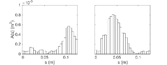
Figure 2: Left: The VT intersections extracted from the test subject during phonation of [] and [i]. Right: The resulting area functions for equation (9), represented as a function of distance from the glottis.

5.1 Area functions for VT and SGT

Solving Webster’s equation requires that the VT is represented with an area function and a centreline, from which curvature information can be computed. Two different VT geometries corresponding to vowels from a healthy 26 years old female are used: A prolonged [] produced at fundamental frequency $f_{o}=168$ Hz and similarly produced [i] at $f_{o}=210$ Hz. These geometries have been obtained by Magnetic Resonance Imaging (MRI) using the experimental setting that has been described in [5]; see also [52, 53, 54] for earlier approaches. The extraction of the computational geometry from raw MRI data has been carried out by the custom software described in [55, 56]. The VT geometries and the area functions are shown in Figure 2, and related VT geometry dependent parameter values are given in Table 1.

The piston model [49, Chapter 7] gives the expression $\theta=2\pi A(L_{VT})/\ell^{2}$ for the normalised acoustic resistance in equation (11) where we use the nominal wavelength $\ell=171.5\,\mathrm{mm}$, corresponding to the centre frequency $2\,\mathrm{kHz}$ of the voice band. The values for $\theta$[], $\theta$[i] together with the resonances $f_{Rj}$[], $f_{Rj}$[i] for $j=1,2$ are given in Table 1. These values of the purely resistive load correspond to an infinitely long, non-resonant waveguide placed in front of the mouth, diameter of which is $95.2\,\textrm{mm}$ for [] and $96.6\,\textrm{mm}$ for [i].

Table 1: Physical and physiological parameters dependent on the VT geometry.

Parameter	[]	[i]
normalised acoustic resistance at mouth, $\theta$	0.064	0.014
area at mouth	299 mm2	66 mm2
VT inertia parameter, $C_{iner}^{VT}$	2540 kg/m4	2820 kg/m4
length of VT, $L_{VT}$	132 mm	136 mm
1st VT resonance, $f_{R1}$, from equations (9)–(11)	749 Hz	199 Hz
2nd VT resonance, $f_{R2}$, from equations (9)–(11)	2084 Hz	2798 Hz

The MRI data that is used for the VT does not cover all of the SGT. For this reason, an exponential horn is used as the subglottal area function for equation (12)

$$A_{s}(s)=A_{s}(0)e^{\epsilon s}\quad\text{ where }\quad\epsilon=\tfrac{1}{L_{SGT}}\ln{\left(\tfrac{A_{s}(L_{SGT})}{A_{s}(0)}\right)}$$ (15)

following [51]. The values for $A_{s}(0)=2\,\mathrm{cm^{2}}$ and $A_{s}(L_{SGT})=10\,\mathrm{cm^{2}}$ are taken from Figure 1 in [51]. The horn length $L_{SGT}$ is tuned so that the lowest subglottal resonance is $f^{\prime}_{R1}=500\,\mathrm{Hz}$ which results in the second lowest resonance at $f^{\prime}_{R2}=1000\,\mathrm{Hz}$. This is a reasonable value for $f_{R1}$ based on Table 1 in [11]; see also [57, 58], [43] and Figure 1 in [28]. The SGT lung termination resistance in equation (12) is given the value $\theta_{s}=1$ which corresponds to an absorbing boundary condition. The air column in this SGT model has a nominal inertia parameter value of 1040 kg/m⁴ which is taken as a guideline for tuning the total inertia of the airways to obtain desirable flow pulse waveforms. For the simulations in this article, $C_{iner}=1.5C_{iner}^{VT}$, where $C_{iner}^{VT}$ refers to the VT inertia parameters given in Table 1.

5.2 Static parameter values

Table 2 lists the numerical values of physiological and physical constants used in all simulations. Note that the vocal fold springs are, for this study, placed symmetrically about the midpoint of the vocal folds. Based on the acoustic reflection and transmission coefficients at the air/tissue interface, the common value of the energy loss coefficients $\alpha_{1}$ and $\alpha_{2}$ in equations (9) and (12), respectively, is taken as

$$\alpha_{1}=\alpha_{2}=\frac{\rho}{\rho_{h}c_{h}}=7.6\cdot 10^{-7}\,\mathrm{\frac{s}{m}}.$$ (16)

All the model parameter values introduced so far are assumed to be equally valid for both female and male phonation, except for vocal fold length $h$. As we are treating female phonation in this article, it remains to describe the parameter values for equations (1) where the differences between female and male phonation are most significant. Horáček et al. provide parameter values for $M$ and $K$ for in male phonation [34, 42] but similar data for female subjects cannot be found in literature. Instead, the masses in $M$ are calculated by combining the vocal fold shape function used in [34] with female vocal fold length reported in [59]. A first estimate for the spring coefficients in $K$ is calculated by assuming that the first eigenfrequency of the vocal folds matches the starting frequency for the simulations. The spring coefficients are then adjusted until simulations produce the desired starting fundamental frequency for the $f_{o}$-glides, giving the constant $K^{0}$ for equations (17)–(18). For details of these rather long calculations, see [33] and [29].

Table 2: Physical and physiological constants.

Parameter	Symbol	Value
speed of sound in air	$c$	343 m/s
density of air	$\rho$	1.2 kg/m3
kinematic viscosity of air	$\mu$	$18.27$ $\mu$N s/m2
vocal fold tissue density	$\rho_{h}$	1020 kg/m3
VT loss coefficient	$\alpha_{1}$	7.6 $\cdot 10^{-7}$ s/m
SG loss coefficient	$\alpha_{2}$	7.6 $\cdot 10^{-7}$ s/m
spring constant in contact (from [34])	$k_{H}$	730 N/m
glottal gap at rest	$g$	0.3 mm
vocal fold length (from [59])	$h$	10 mm
vocal fold thickness (from [34])	$L$	6.8 mm
superior vocal fold spring location (from [33])	$l_{1}$	0.85
inferior vocal fold spring location (from [33])	$l_{2}$	0.15
control area height below glottis	$H_{0}$	11.3 mm
control area height above glottis	$H_{1}$	2 mm
equivalent gap length for viscous loss in glottis	$L_{g}$	1.5 mm
SGT length	$L_{SGT}$	350 mm
normalised acoustic resistance at lungs	$\theta_{s}$	1
glottal entrance/exit coefficient	$k_{g}$	0.2
subglottal (lung) pressure over the ambient	$p^{0}_{sub}$	650 Pa

Let us conclude with a sanity check on the parameter magnitudes for equation (1) describing the vocal folds. The total vibrating mass for female phonation is $m_{1}+m_{2}+m_{3}=0.27\ \mathrm{g}$ and the total spring coefficients are $k_{1}+k_{2}=216\ \mathrm{N/m}$. These nominal values yield $f_{o}\approx 150$ Hz for female phonation. If the characteristic thickness of the vocal folds is assumed to be about $5\ \mathrm{mm}$, these parameters yield a magnitude estimate for the elastic modulus of the vocal folds by $E\approx\frac{k_{1}+k_{2}}{Lh}\cdot 5\cdot 10^{-3}\ \mathrm{m}\approx 15.9\ \mathrm{kPa}$. This should be compared to Figure 7 in [60] where estimates are given for the elastic modulus of ex vivo male vocal folds and values between $2.0\ \mathrm{kPa}$ and $7.5\ \mathrm{kPa}$ are proposed for different parts of the vocal fold tissue.

6 Computational Aspects

6.1 Parameter control for obtaining vowel glides

The $f_{o}$-glide is simulated by controlling two parameter values dynamically. First, the matrix $K$ is scaled while keeping the matrix $M$ constant. This approach is based on the assumption that the vibrating mass of vocal folds is not significantly reduced when the speaker’s pitch increases; a reasonable assumption as far as register changes are excluded. It should be noted that the relative magnitudes of $M$ and $K$ essentially determine the resonance frequencies of model (1). However, attention must be paid to their absolute magnitudes using, e.g., dimensional analysis since otherwise the load terms $F_{j}(t)$ in equation (1) (containing the aerodynamic forces, contact force between the vocal folds during the glottal closed phase, and the counter pressure from the VT/SGT) would scale in an unrealistic manner.

The subglottal pressure, $p_{sub}$, is the second parameter used to control the glide production. The dependence of the fundamental frequency on $p_{sub}$ has been observed in simulations [10, 61], physical experiments using upscaled replicas [14], as well as in humans [62] and excised canine larynges [63]. The impact of $p_{sub}$ on $f_{o}$ is, however, secondary in these glides ($f_{o}$ trajectories are within a few Hz). Instead, $p_{sub}$ is scaled in order to maintain phonation and to prevent large changes in phonation type as the stiffness of the vocal folds changes. The scaling parameter value of 2 was found by trial and error to maintain the glottal open quotient $OQ$ (proportion of glottal cycle during which the glottis is open), the closing quotient $ClQ$ (proportion of the glottal cycle during which the flow is decreasing), and the maximum of $\Delta W_{1}$ approximately steady over the upward glide when acoustic feedback was disabled.

The parameters are scaled exponentially with time

$$K(t)=2.2^{2t/T}K^{0},\quad p_{sub}(t)=2^{t/T}p^{0}_{sub}$$ (17)

for rising glides, and

$$K(t)=2.2^{2-2t/T}K^{0},\quad p_{sub}(t)=2^{1-t/T}p^{0}_{sub}$$ (18)

for falling glides. The duration of the glide is $T=3\,\mathrm{s}$, and $t$ is the time from the beginning of the glide. Note that the temporal scale of the glides is long compared to glottal cycles, and hence the control parameters $K$ and $p_{sub}$ can be regarded as static from the point of view of the vocal fold dynamics. Other starting conditions (particularly, vocal fold displacements and velocities, and pressure and velocity distributions in the resonators) are taken from stabilised simulations. These parameters produce glides with $f_{o}$ approximately in the range $[150\,\mathrm{Hz},320\,\mathrm{Hz}]$, although the exact range depends on the VT geometry and vocal fold damping as well.

The damping parameters $b_{i}$ for $i=1,2,$ in equation (2) play an important but problematic role in glottis models. If there is too much damping (while keeping all other model parameters fixed), sustained oscillations do not occur. Conversely, too low damping will cause instability in simulated vocal fold oscillations. The magnitude of physically realistic damping in vibrating tissues is not available, and the present model could possibly fail to give a quasi-stationary glottis signal even if realistic experimental damping values were used. With some parameter settings, the model even produces quasi-stationary signal at several damping levels. For simplicity, we set $b_{i}=\beta>0$ for $i=1,2$, and use golden section search to find at least one value of vocal fold loss $\beta$ that results in stable, sustained oscillation. The damping remains always so small that its lowering effect on the resonances of the mass-spring system (1) is negligible.

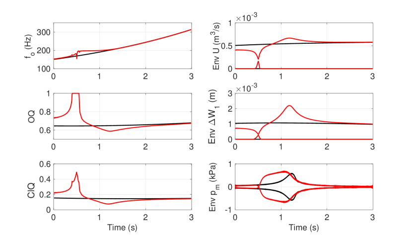
Figure 3: Glide for vowel [i] with $Q_{pc}=0.1$ and $\beta=0.012\,\textrm{kg/s}$ (red) and the same glide without VT and SGT feedback ($Q_{pc}=0$) (black). Left: fundamental frequency ($f_{o}$), open quotient ($OQ$), and closing quotient ($ClQ$). Right: Envelopes of volume flow ($U$), glottal opening ($\Delta W_{1}$), and sound pressure at lips ($p_{m}$). The values of $f_{o}$, $OQ$, and $ClQ$ have been extracted pulse by pulse from the volume flow signal.

6.2 Numerical realisation

The model equations are solved numerically using MATLAB software and custom-made code. The vocal fold equations of motion (1) are solved by the fourth order Runge–Kutta time discretisation scheme. The flow equation (5) is solved by the backward Euler method. The VT and SGT are discretised by the FEM using piecewise linear elements ($N=29$ for VT and $N=10$ for SGT) and the physical energy norm of Webster’s equation. Energy preserving Crank–Nicolson time discretisation (i.e., Tustin’s method [64]) is used. The time step is almost always $10\ {\mu s}$ which is small enough to keep the frequency warping in Tustin’s method under one semitone for frequencies under $13\mathrm{kHz}$. Reduced time step, however, is used near glottal closure. This is due to the discontinuity in the aerodynamic force in equation (8) at the closure which requires numerical treatment by interpolation and time step reduction as explained in Section 2.4.1 of [33].

Solving the equations of motion of the vocal folds is the computationally most expensive part of the model, taking approximately 55% of the running time in simulations of steady phonation with given parameter values. In comparison, solving the Webster’s equations with precomputed mass, stiffness, and loss matrices takes approximately 10% of the simulation time, and the flow equation solver less than 2%.

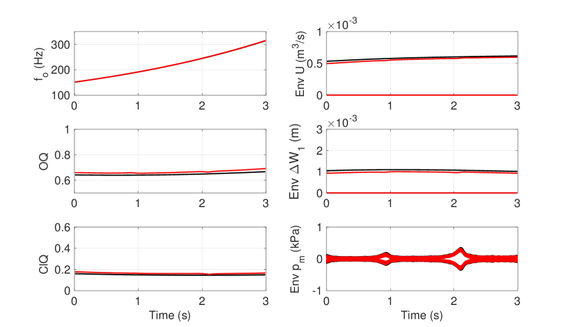
Figure 4: Glide for vowel [] with $Q_{pc}=0.1$ and $\beta=0.012\,\textrm{kg/s}$ (red) and the same glide without VT and SGT feedback ($Q_{pc}=0$) (black). Left: fundamental frequency ($f_{o}$), open quotient ($OQ$), and closing quotient ($ClQ$). Right: Envelopes of volume flow ($U$), glottal opening ($\Delta W_{1}$), and sound pressure at lips ($p_{m}$). $f_{o}$, $OQ$, and $ClQ$ have been extracted pulse by pulse from the volume flow signal.

7 Simulation Results

The results of upward glide simulations for vowels [, i] are shown in Figures 3–4. The fundamental frequency $f_{o}$ trajectory as well as glottal open quotient $OQ$ and closing quotient $ClQ$ have been extracted from the glottal volume flow $U$ signal pulse by pulse in all figures. Envelopes of $U$, glottal opening $\Delta W_{1}$, and pressure signal at lips $p_{m}$ are also displayed.

The simulations indicate a consistent locking pattern at $f_{R1}[{\tipaencoding i}]$ in $f_{o}$ trajectories that vanishes if the VT feedback is decoupled by setting $Q_{pc}=0$. The locking pattern in rising glides follows the representation given in Figure 6 (right panel): sudden jump upwards to $f_{R1}$, a locking to a plateau level, and a smooth release. Such locking behaviour is not observed for glides of [] where $f_{R1}$[] is not inside the simulated frequency range $[150\,\mathrm{Hz},320\,\mathrm{Hz}]$. The vocal tract resonance fractions $f_{R1}$[]$/4=187\,\mathrm{Hz}$ and $f_{R1}$[]$/3=250\,\mathrm{Hz}$, are within the frequency range, and the corresponding events are visible in the sound pressure signal at the lips; see Figure 4. They do not, however, cause noticeable changes in the $f_{o}$ trajectory of the glottal flow.

The frequency jump at $f_{R1}[{\tipaencoding i}]$ in the simulations is preceded by a decrease in vocal fold oscillation and glottal flow amplitudes. This is accompanied by the disappearance of full glottal closure ($OQ=1$) and less sharp decrease in glottal flow during closure (higher $ClQ$), both of which indicate increased breathiness of the phonation. The locking plateau coincides with a nearly constant rate of decreasing $OQ$ and $ClQ$, and after the release of $f_{o}$ the parameters return to the feedback free trajectories.

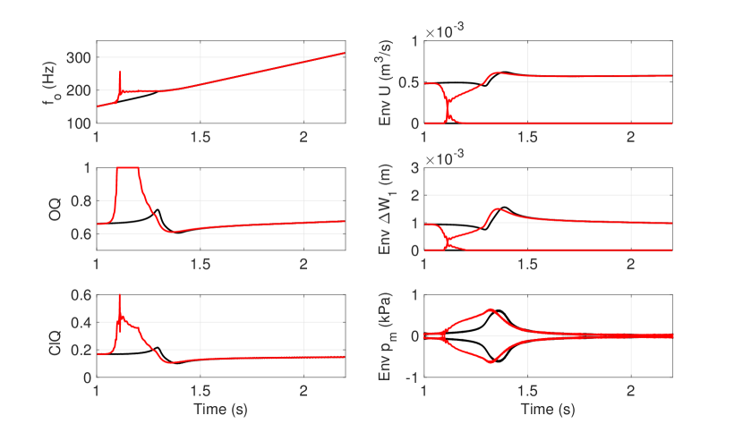
Figure 5: Upward (black) and downward (red) glides for vowel [i] with $Q_{pc}=0.04$ and $\beta=0.012\,\textrm{kg/s}$. Left: fundamental frequency ($f_{o}$), open quotient ($OQ$), and closing quotient ($ClQ$). Right: Envelopes of volume flow ($U$), glottal opening ($\Delta W_{1}$), and sound pressure at lips ($p_{m}$). On the x-axis, relative vocal fold stiffness refers to the coefficient of the $K^{0}$ matrix in equations (17) and (18).

Keeping $Q_{pc}$ and other model parameters the same, a falling $f_{o}$ glide shows a significantly more pronounced or longer locking at $f_{R1}$ compared to rising glides; see Figure 5. Note that in Figure 5 the x-axis is the relative vocal fold stiffness, which for rising glides is $2^{t/T}$ and for falling glides $2^{1-t/T}$ as given in equations (17) and (18). The fluctuations in $f_{o}$ in the falling glides around the "corner" of the lock and at frequencies below this are qualitatively similar to what occurs at extreme values of $Q_{pc}$ and $\beta$ for rising glides. In contrast, fluctuations in the lip pressure envelope occur temporally after the release of the locking in both rising and falling glides.

Finally, the effect of model parameters $\beta$ and $Q_{pc}$ on the glide simulations at $f_{R1}$[i] is considered. These observations are qualitatively described in Figure 6. In the right panel, the medium values for $\beta$ refer to the interval $[0.01,0.02]$ and for $Q_{pc}$ to the interval $[0.05,0.1]$. These intervals can thus be regarded as feasible parameter ranges for vowel glide simulations of [i].

Referring to Figure 6 (right panel), the full frequency range $[150\,\mathrm{Hz},320\,\mathrm{Hz}]$ for $f_{o}$ can be obtained with modal locking as shown in Figure 3 if both $Q_{pc}$ and $\beta$ have medium values or if one is high and the other low. If both parameters are high or one is high and other medium, the simulated $f_{o}$ range is reduced to above $200\,\mathrm{Hz}$ which is the value of $f_{R1}$[i]. This glide starting frequency cannot be lowered by changing $K$, and it appears to represent very strong modal locking at the onset of the vowel glide simulation.

The stability of glide simulations (understood as slowly changing amplitude envelope of glottal volume flow $U$) becomes a serious issue at low and high values of $\beta$. We have tuned the subglottal pressure $p_{sub}$ in glide simulations as given in equations (17)–(18). If $p_{sub}$ were instead kept constant, we would observe an increasing $OQ$ and decreasing amplitudes of glottal flow and vocal fold oscillations throughout the glide but the qualitative behaviour of modal locking events, including the behaviour of phonation type parameters around these events, remains very similar.

8 Sensitivity and Robustness

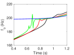
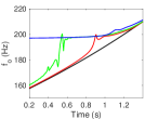
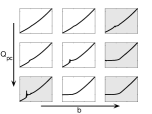
Figure 6: Left: $f_{o}$ trajectories for [i] fixed $Q_{pc}=0.1$ and different values of $\beta$: black $0.005\,\textrm{kg/s}$, red $0.01\,\textrm{kg/s}$, green $0.015\,\textrm{kg/s}$, and blue $0.03\,\textrm{kg/s}$. Middle: $f_{o}$ trajectories for [i] with $\beta=0.012\,\textrm{kg/s}$ and different values of $Q_{pc}$: black $0.0$, red $0.05$, green $0.1$, and blue $0.25$. Right: $f_{o}$ trajectories for [i] qualitatively as $Q_{pc}$ and $\beta$ increase in the direction of the arrow. Light gray background indicates that small parameter changes can lead to loss of quasi-stable glides.

Parameter tuning of the vowel model is tricky business as can be seen from model parameter optimisation experiments described in Chapter 4 in [29]. By exaggerating some of the parameter values, it is possible to make vowel glide simulations over $f_{R1}$[i] behave in a way that can be excluded by experiments or observations from natural speech.

In phonetically relevant simulations, various tuning parameters must be kept in values that are not only physically reasonable but also do not produce obviously counterfactual predictions. When such a realistic operating point has been found, it remains to make sure that the simulations give consistent and robust results near it. In doing so, we also check which parts of the full model are truly significant for the model behaviour reported above.

8.1 Acoustics of the vocal tract by Webster’s equation

The constants $\alpha_{1}$ and $\alpha_{2}$ in respective equations (9) and (12) regulate the boundary dissipation at the air/tissue interface. As shown in Section 3 in [46], the same parameter appears in the corresponding dissipating boundary condition $\alpha\phi_{t}+\bar{\nu}\cdot\nabla\phi=0$ for the wave equation $\phi_{tt}=c^{2}\Delta\phi$ where $\phi$ is the 3D acoustic velocity potential and $\bar{\nu}$ denotes the exterior normal of the VT/air boundary. The qualitative effect of physically realistic tissue losses to vowel glide simulations was observed to be insignificant; see also Section 5 in [26]. However, these losses move slightly the VT resonance positions computed from equations (9).

On the other hand, the VT resonances are quite sensitive to the normalised acoustic resistance $\theta$ in equation (11). This parameter regulates the energy loss through mouth to the external acoustic space, and its extreme values $0$ and $\infty$ correspond to open and closed ends for idealised acoustic waveguides, respectively. Again, physically realistic variation in $\theta$ does not change the qualitative behaviour of vowel glides near $f_{R1}$[i] as reported above.

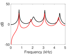
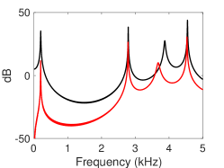
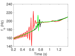
Figure 7: Left and middle: The frequency responses of the VT acoustic loads for [] and [i], computed from Webster’s equation (9). The black curves are the responses using the purely resistive load of equation (11) at the mouth where the parameter values are given in Table 1. The responses using the RL impedance model and its nominal parameter values in Table 3 are shown in red. Right: Ringing at a modal locking event of [i] shown for both types of loads at the mouth: purely resistive load (black) and RL model load using nominal and tuned parameter values (red and green, respectively). The parameter values for the RL impedance model are given in Table 3.

To consider the effect of the reactive acoustic loading at the mouth opening, a first order impedance model was used, based on a parallel coupling of a resistive load $R$ and an inductive load $L$. The nominal values for $R$ and $L$ in Table 3 were obtained by interpolation at $200\,\textrm{Hz}$ from the piston model given in [49, Chapter 7, Eq. (7.4.31)]. The transfer function $Z(s)=\frac{sRL}{R+sL}$ approximates the irrational piston model impedance very well for frequencies under $2\,\textrm{kHz}$, and the frequency responses in Figure 7 (left and middle panels) are reasonable as well.

Table 3: Values for the parameters of the RL impedance model and its transfer function.

Parameter	[]	[i]
Nominal value of $R$	$1.98\cdot 10^{6}\frac{\textrm{kg}}{\textrm{s m}^{4}}$	$8.96\cdot 10^{6}\frac{\textrm{kg}}{\textrm{s m}^{4}}$
Nominal value of $L$	$33.2\frac{\textrm{kg}}{\textrm{m}^{4}}$	$70.6\frac{\textrm{kg}}{\textrm{m}^{4}}$
Tuned value of $R$	(Not required.)	$8.96\cdot 10^{4}\frac{\textrm{kg}}{\textrm{s m}^{4}}$
Nominal value of $Z(400\pi i)$	$879+4.17\cdot 10^{4}i$	$879+8.87\cdot 10^{4}i$

However, the value $\lim_{s\to+\infty}{Z(s)}=R$ overestimates its piston model counterpart by over 700 %, and the vowel simulations show excessive ringing, e.g., at modal locking events as shown in Figure 7 (right panel). In a low-order rational model, all of the lumped inductance appears at the mouth opening whereas the inductance is distributed by resistive shunting and transmission delays to an infinite volume in the piston model. Hence, the value of $R$ must be tuned down from its nominal value so as not to contradict experimental evidence.

Another low-order time-domain model for termination, based on an idealised spherical interface at a horn opening, is proposed in [50, Eq. (39)]. In its most general form, the model is an integro-differential delay equation with nine parameters and a single delay lag. Unfortunately, the general form cannot be introduced to Webster’s model as a boundary condition: this is the salient feature of the parallel RL model (having the same circuit topology as the first-order high pass model [50, Eq. (28)]) that simplifies the implementation of the FEM solver.

The role of the VT curvature in equation (9) is involved, too. As can be seen from equation (10), the curvature results in a second order correction in the curvature ratio $\eta$ to the speed of sound $c$ in equation (9). In waveguides of significant intersectional diameter compared to wavelengths of interest, the contribution of $\eta$ in equation (10) appears to be secondary to a larger error source that is related to curvature as well. This is caused by the fact that a longitudinal acoustic wavefront does not propagate in the direction of the geometric centreline of a curved waveguide even if the waveguide were of circular intersection with constant diameter. The wavefront has a tendency to “cut the corners” in a frequency and geometry dependent manner, and we do not have a mathematically satisfying description of the “acoustically correct” centreline that would deal with this phenomenon optimally in the context of Webster’s equation. Extraction of the area function $A(\cdot)$ for equation (9) from MR images, however, requires some notion of a centreline, and using a different centreline would lead to slightly different version of $A(\cdot)$. This would somewhat change, e.g., the resonance frequencies of equation (9) but not the mathematical structure of the model nor the results of vowel glide simulations. Hence, we simply use the area functions and centrelines obtained from 3D MR images by the custom code described in [56] using its nominal settings.

It remains to consider the non-longitudinal resonances of the VT. By its construction, the generalised Webster’s equation does not take into account at all the transversal acoustic dynamics of the VT. It is known from numerical 3D Helmholtz resonance experiments on several dozens of VT geometries that lowest non-longitudinal resonances of the human VT tract are at approximately $4\,\mathrm{kHz}$ corresponding to $\lambda/2\approx 4\,\mathrm{cm}$; see, e.g., [5] and [55]. Anatomically, such length may appear between opposing valleculae, piriform fossae, or even across the mouth cavity in some VT vowel configurations. However, the upper limit of $4\,\mathrm{kHz}$ for Webster’s equation is adequate for the computation of the acoustic counter pressure $p_{c}$ in equation (13) for several octaves lower fundamental frequencies $f_{o}\in[150\,\mathrm{Hz},320\,\mathrm{Hz}]$ that are used in vowel glide simulations.

8.2 Subglottal acoustics

To large extent, what was stated above about the modelling error of the VT acoustics applies to the SGT acoustics as well. We complement this treatment by considering how and to what extent subglottal acoustics plays a role in the vowel glide simulations reported above

Even though the acoustic termination at lungs is strongly resistive (see [65]), significant ringing (i.e., oscillatory response to an abrupt change of a forcing) takes place in the subglottal space. In simulations, it is seen in the bottom panels of Figure 8. Moreover, it has been verified by in vivo measurements [57, 58, 66, 12], using physical models [11, 67], and by mathematically modelling the subglottal acoustics [28] based on anatomic data of trachea and the progressively subdividing system of bronchi and the alveoles [68, 69]. A refined model for subglottal acoustic impedance was developed in [65] for the branching airway network in terms of transmission line theory, taking into consideration the contribution from yielding walls due to material parameters of cartilages and soft tissues.

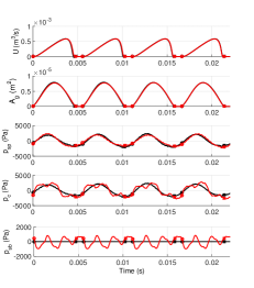
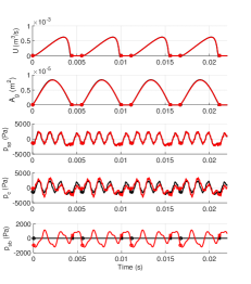
Figure 8: Left: Volume flow ($U$), glottal area ($A_{g}=\Delta W_{1}h$), supraglottal pressure ($p_{sp}$) just superior to the vocal folds, counter pressure ($p_{c}$), and subglottal pressure just inferior to the vocal folds ($p_{sb}$) without SGT (black line) and with SGT (red line) for the vowel [i] at $f_{o}=180$ Hz. Glottal closure are indicated by squares and openings by circles. Right: Similar signals for the vowel [].

During the open phase, the inertia of the air column from bronchi up to mouth opening is taken into account by $C_{iner}$ in equation (5). At closure, the flow velocity $v_{o}$ drops to zero, and a rarefaction pulse is formed above the vocal folds due to air column inertia in the VT, and this is part of the acoustics modelled by equation (9). Similarly, a compression pulse is formed below the vocal folds, known as the “water hammer” in [70]. The subglottal resonator equation (12) is mainly excited by the water hammer. Both of these pulses can be seen in the supra- and subglottal pressure signals $p_{sp}$ and $p_{sb}$ in Figure 8.

The water hammer is the most important component of subglottal ringing, accompanied by its first echo that arrives back to vocal folds after approximately $2\,\mathrm{ms}$ delay. The delay corresponds to the lowest subglottal formant between $500\,\mathrm{Hz}$ and $600\,\mathrm{Hz}$ as reported in [58] and [28]. The first echo returns during the glottal closure at least if $f_{o}<150\,\mathrm{Hz}$ and the open quotient (OQ) of the pulse does not exceed $50$ %; see Figure 4 in [57] for measurements and Figure 12 in [28] for simulations. The echoes of the water hammer pulse can be clearly seen in Figure 8 as well but now the first echo returns after the glottis has opened again due to higher values of $f_{o}$ and OQ in these simulations.

The observations from simulations indicate that the subglottal acoustics has an observable effect on glottal pulse waveform. The subglottal effect will get more pronounced when $f_{o}\to f^{\prime}_{R1}=500\,\mathrm{Hz}$ which is the predefined frequency of the first subglottal resonance. This can be understood in terms of the supraglottal behaviour shown in Figure 8 since both the VT and the SGT resonators have been realised similarly within the full model. The sensitivity of the $f_{o}$ trajectory in the range $[150\,\mathrm{Hz},320\,\mathrm{Hz}]$ for the subglottal effect depends on the magnitude of the SGT component of the counter pressure, regulated by the parameter $c_{3}$ in equation (13). Considering the model behaviour at supraglottal resonance fractions of $f_{R1}$[], it is to be expected that the first subglottal resonance fraction $f^{\prime}_{R1}/2$ should show up similarly. This, indeed, happens if the coupling constant $c_{3}$ in equation (13) is large.

8.3 Flow model

The glottal flow described by equations (5)–(6) contains terms representing the effect of viscosity in the glottis as well as pressure loss and recovery at the entrance and exit of the glottis, respectively. Viscous pressure loss can easily be seen to be significant by considering the glottal dimensions and viscosity of air in the first term of equation (6). It is clear from this equation that the viscous losses dominate at least if the glottal opening is small.

The importance of entrance and exit effects during parts of the glottal open phase can be seen, for example, by comparing simulated volume velocities and glottal opening areas with the experimental curves in Figure 3 in [44], obtained from a physical model of the glottis. In model simulations, leaving out this transglottal pressure loss term changes the glottal pulse waveform significantly if other model parameters are kept the same, as shown in Figure 3.7 in [29]. About half of the total pressure loss in simulations is due to entrance and exit effects at the peak of opening of the glottis; see Figure 3.6 in [29]. However, the behaviour of the simulated $f_{o}$ trajectories over $f_{R1}$[i] does not change if the transglottal pressure loss term is removed. Then, however, the vowel glide must be produced by different model parameter values.

9 Discussion

We have reported observations on the locking of simulated $f_{o}$ glides on a resonance of the VT. The locking behaviour shows a consistent time-dependent behaviour that is similar for rising and falling glides. The $f_{o}$ jump at the beginning of the locking in rising glides and end of the locking in falling glides occurs together with and increased breathiness of phonation as characterised by open quotient $OQ$ and closing quotient $ClQ$. During the locking plateau, these parameters indicated an approximately steady change of phonation type.

The locking takes place only at frequencies determined by sub- or supraglottal resonances. Use of $p_{sub}$ as a secondary control parameter for the glides ensure that the main cause for changes in $OQ$ and $ClQ$ is the acoustic loading. By modifying the strength of the acoustic feedback (i.e., the parameter $Q_{pc}$ in equation (13)) and vocal fold tissue losses (i.e., the parameter $\beta$), the locking tendency at $f_{R1}$[i] may be modulated from non-existent (where both $Q_{pc}$ and $\beta$ have low values) to extreme locking at $f_{R1}$[i] without release (where $Q_{pc}$ and/or $\beta$ have exaggeratedly large values); see Figure 6. By decoupling secondary components from the simulation model, the locking behaviour at $f_{R1}$[i] remains the same, even though the model parameter values required for the desired glottal waveform change. We conclude that the simulation results on vowel glides reported above reflect the model behaviour in a consistent and robust manner.

Vowel glides observed in test subjects are another matter. Any model is a simplification of reality, and there is a catch in assessing the role of unmodelled physics: a proper treatment would require the modelling of it. Short of this, we discuss these aspects based on literature, model experiments, and reasoning by analogy.

9.1 Acoustics

Viscosity of air has not been taken into account in the acoustics model though a measurable effect is likely take place in narrow parts of the VT or SGT. Resulting attenuation can be treated by adding a dissipation term of Kelvin–Voigt type to equations (9) and (12). For a constant diameter waveguide, the term is proportional to $\mu\psi_{sst}/c^{2}$. Adding viscosity losses will widen and lower the resonance peaks of Webster’s resonators (i.e., lower their Q-value), with a slight change in the centre frequencies. An analogous effect can be studied by increasing the tissue dissipation parameter $\alpha_{1}$ in equation (9) (or $\alpha_{2}$ in equation (12)) to a very high value which has been observed not to change the conclusions on vowel glide simulations. Similarly, the overall acoustic resistance of the VT has no qualitative effect which can be seen in [71] where the modal locking was observed for vowel [œ] at the lowest resonance $647\,\mathrm{Hz}$ despite the fact that the anatomic geometry of [œ] has a much wider flow channel than that of [i].

The SGT modelling by the horn is a crude simplification of the fractal-like lower airways and lungs. The network structure of the subglottal model in [28] could be replicated by interconnecting a large number of Webster’s resonators, each modelled by equation (12). The resulting transmission graph is a passive dynamical system by Section 5 in [72], but it is not clear how to write an efficient FEM solver for such configurations.

The model proposed in [28] as well as the transmission graph approach are likely to produce the correct resonance distribution and frequency-dependent energy dissipation rate at the lung end without tuning. The horn model does require tuning of the horn opening area and the boundary condition on it in order to get realistic behaviour on the lowest subglottal resonance $f^{\prime}_{R1}=500\,\mathrm{Hz}$. Doing so freezes all the higher subglottal resonances at fixed positions, e.g., $f^{\prime}_{R2}=1\,\mathrm{kHz}$. The branching subglottal models given in Figure 8 in [28] have the second subglottal resonance between $1.3\,\mathrm{kHz}$ and $1.5\,\mathrm{kHz}$. It was observed in [65] that the soft tissues introduce an additional resonance to the subglottal system that is lower than the first subglottal formant $F^{\prime}_{1}$ due to air column dynamics. The is no obvious way how a horn model could be used to accommodate such a resonance at $\approx 350\,\mathrm{Hz}$ due to the yielding wall dynamics.

Based on the observations on the simulated vowel glides, it seems convincing that the overall subglottal effect on the fundamental frequency $f_{o}$ is insignificant for vowel glides within $[150\,\mathrm{Hz},320\,\mathrm{Hz}]$ that is over $100\,\textrm{Hz}$ away from $f^{\prime}_{R1}$. However, the subglottal effect is certainly discernible in waveforms as in Figure 8, but the effect of higher subglottal resonances $f^{\prime}_{R2},f^{\prime}_{R3},\ldots$ cannot be seen even there. In current simulations of female phonation, the vocal fold mass-spring system has its mechanical resonances at approximately $150\,\mathrm{Hz}$, which acts as a low-pass filter for subglottal excitation in higher frequencies. The same conclusions are likely to hold when using a more complicated subglottal resonator geometry with one caveat: a graph-like subglottal geometry has lots of cross-mode resonances that affect the subglottal acoustic impedance in other ways than just moving the pole positions.

Also the DC-component of the glottal flow loads the acoustic resonators in equations (11) and (12). If we use $v_{ac}(t)=v_{0}(t)-\frac{1}{T}\int_{t-T}^{t}{v_{0}(\tau)\,d\tau}$ with $T=2/f_{o}$ instead of $v_{0}$ as input to the resonator equations, only negligible effects are observed in simulated stable waveforms. There are more pronounced effects in the beginnings of simulated phonation when a stable waveform has not yet developed.

9.2 Vocal fold geometry and glottal flow

The idealised vocal folds geometry shown in Figure 1 (right panel) leads to a particularly simple expression for the aerodynamic force in equation (8). Replacing the sharp peaks by flat tops in Figure 1 (but keeping the same glottal gap $g$ at rest) results in phonation that has typically lower open quotient (OQ) whereas the original wedge-like geometry produces more often phonation where the glottis does not close. This change makes it easier to adjust the parametrisation of the model to obtain some phonation targets. In particular, the glottal loss parameter $k_{g}$ can be set closer to more commonly used, somewhat larger values since the model geometry becomes more similar to the geometries used in related literature.

Another aspect involving the aerodynamic force on vocal fold structures is associated with the hydrostatic pressure reference level in vibrating tissues. This level is denoted by $p_{ref}$, and it is expected to satisfy $p_{ref}\leq p_{sub}$. If the air pressure between the vocal folds were equal to $p_{ref}$, then the vocal fold wedges would not be accelerated by the pressure difference. In equation (7), we use $p_{ref}=p_{sub}$, and we always have $p(x,t)-p_{sub}\leq 0$. For this reason, the effect of the aerodynamic force is always trying to close the glottis in this case. For small flow velocities $V(x,t)$, using $p(x,t)-p_{ref}$ with $p_{ref}<p_{sub}$ in equation (7) would give the following outcome: the driving pressure $p_{sub}$ would push the vocal folds open more strongly than the aerodynamic force would pull them close. Unfortunately, there is no obvious way to determine the true magnitude of $p_{ref}$ as it is an outcome of dynamic pressure equalisation processes related to $p_{sub}$ and the additional partial pressure due to haemodynamics in tissues. Using a tuned value of $p_{ref}$ instead of $p_{sub}$ in equation (7) would be desirable, e.g., in phonation onset simulations; in particular, if $g=0$ where using $p_{ref}=p_{sub}$ would not start a phonation cycle at all.

The glottal flow has been studied extensively since 1950’s. Compared to the flow model given above, physiologically more faithful glottal flow solvers have been proposed in, e.g., [37], [73] and [74]; see also [51], [10], [75], and [44]. As pointed out in [75], more sophisticated flow models are challenging to couple to acoustic resonators since the interface between the flow-mechanical (in particular, the turbulent) and the acoustic components is no longer clearly defined.

Flow separation and Coandă effect during the diverging phase of the phonatory cycle (which obviously cannot occur in wedge-like geometry of Figure 1) have been studied in [74], [76] and [37] using boundary layer theory and physical model experiments. The boundary layer leaves the vocal fold surfaces at the time-dependent flow separation point, say $x_{s}$, forming a jet which extends downstream into supraglottal space. Thus, the vocal folds “stall” at $x_{s}$, and the aerodynamic force on them is greatly diminished; see Section IV in [74] where the vocal fold model is from [77]. Similarly, the viscous pressure loss equation (A7) in [37] depends only on the upstream part of glottis that ends at $x_{s}$. Simplifying assumptions on the vocal fold geometry [37] are required for computing $x_{s}$, and the result is sensitive to the geometry which makes it challenging to model.

Turbulence in supraglottal space is a spatially distributed acoustic source, and it does not provide a scalar flow velocity signal for boundary control as $v_{0}$ in equation (11). The supraglottal jet may even exert an additional aerodynamic force to vocal folds that would not be part of the acoustic counter pressure $p_{c}$ from the acoustic resonators. Turbulence in VT constrictions is the primary acoustic source for unvoiced fricatives, and many such sources have been modelled separately in, e.g., [51]. Much of the turbulence noise energy lies above $4\,\mathrm{kHz}$ but Webster’s model equation (9) is an accurate description of VT acoustics only below $4\,\mathrm{kHz}$ due to the lack of cross-modes [78, 79]. This fact speaks against the wisdom of including turbulence noise in the proposed model.

The proposed phonation model treats flow-mechanical and acoustic components using separate equations, and we conclude that this paradigm is not conducive for including the advanced flow-mechanical features discussed above. Instead, phonation models based on Navier–Stokes equations would be a more appropriate framework.

10 Conclusions

We have presented a model for vowel production, based on (partial) differential equations, that consists of submodels for glottal flow, vocal folds oscillations, and acoustic responses of the VT and subglottal cavities. The model has been originally designed as a tunable glottal pulse source for a high-resolution VT acoustics simulator that is based on the 3D wave equation and VT geometries obtained by MRI as explained in [5, 55]. The model has found applications as a controlled source of synthetic vowels that are needed in, e.g., developing speech processing algorithms such as the inverse filtering [6, 7].

In this article, the model was used for simulations of rising and falling vowel glides of [, i] in frequencies that span one octave $[150\,\mathrm{Hz},320\,\mathrm{Hz}]$. This interval contains the lowest VT resonance $f_{R1}$ of [i] but not that of []. Perturbation events in simulated vowel glides were observed at VT acoustic resonances, or at some of their fractions but nowhere else. The fundamental frequency $f_{o}$ of the simulated vowel was observed to lock to $f_{R1}$[i] but similar locking was not seen at any of the resonance fractions. The locking events were accompanied by changes in the phonation: increased breathiness below and partially at the locking frequency and steady change in breathiness during most of the lock. Such modal locking event takes place only when the acoustic feedback from VT to vocal folds is present, and then it has a characteristic time-dependent behaviour. A large number of simulation experiments were carried out with different parameter settings of the model to verify the robustness and consistency of all observations.

To what extent do the simulation results validate the proposed model? The model produces perturbations of the glottal pulse both at VT resonances and at some of the VT resonance fractions. Of the former, a wide existing literature was reviewed in Introduction. Observations on the subformant perturbations in speech have not been reported, to our knowledge, in experimental literature. There is a particular temporal pattern of locking in simulated perturbations at $f_{R1}$[i] as explained in Figure 6 (left panel). Although pulse based $f_{o}$ trajectories are rarely shown in literature, a similar pattern can be seen in the speech spectrograms given in Figure 5 in [19], and Figure 4 in [18], as well as in vowel glide samples in the data set of the companion article [3]. A similar locking behaviour can also be seen in simulated spectrograms in Figure 6 in [80] and Figures 13 and 14 in [16], and it can also be interpreted to lie behind the experimental results shown in Figures 10b and 13b of [14]. The glottal flow and area simulations in Figure 8 are remarkably similar with the experimental data presented in Figures 4-7 in [57], the signals produced by different numerical models (see Figures 14a-14c in [10], Figures 8 and 10 in [43], Figures 10–11 in [28], Figure 6 in [73], Figure 5 in [81]), and the glottal pulse waveforms obtained by inverse filtering in, e.g., Figures 10–13 in [6], Figures 5.3, 5.4, and 5.17 in [82], [83], and Figures 3 and 6 in [7].

The simulation model does not include the neural control actions on the vocal fold structures or dynamic modifications of the VT geometry. There is also a significant control action affecting the subglottal pressure and it has been used as a control variable in equations (17)–(18) for glide productions. In humans, neural control actions are part of feedback loops, of which some are auditive, and some others operate directly through tissue innervation and the central nervous system. So little is known about these feedback mechanisms that their explicit mathematical modelling seems infeasible. Instead, the model parameters for simulations are tuned so that the simulated glottal pulse waveform corresponds to experimental speech data. Despite these simplifications the model appears to be sufficiently detailed to replicate the observations found in literature.

References

- [1] T. Chiba, M. Kajiyama, The vowel, its nature and structure, Phonetic Society of Japan, Tokyo, 1941.
- [2] G. Fant, Acoustic theory of speech production, Mouton, The Hague, 1960.
- [3] D. Aalto, J. Malinen, M. Vainio, Modal locking between vocal fold and vocal tract oscillations: Experiments and statistical analysis, Tech. rep., arXiv:1211.4788 (2013).
- [4] I. R. Titze, R. J. Baken, K. W. Bozeman, S. Granqvist, N. Henrich, C. T. Herbst, D. M. Howard, E. J. Hunter, D. Kaelin, R. D. Kent, J. Kreiman, M. Kob, A. L’́ofqvist, S. McCoy, D. G. Miller, H. Noé, R. C. Scherer, J. R. Smith, B. H. Story, J. G. Švec, S. Ternstr’́om, J. Wolfe, Toward a consensus on symbolic notation of harmonics, resonances, and formants in vocalization, The Journal of the Acoustical Society of America 137 (5) (2015) 3005–3007. doi:10.1121/1.4919349.
- [5] D. Aalto, O. Aaltonen, R.-P. Happonen, P. Jääsaari, A. Kivelä, J. Kuortti, J.-M. Luukinen, J. Malinen, T. Murtola, R. Parkkola, J. Saunavaara, T. Soukka, M. Vainio, Large scale data acquisition of simultaneous MRI and speech, Applied Acoustics 83 (2014) 64–75. doi:10.1016/j.apacoust.2014.03.003.
- [6] P. Alku, Glottal wave analysis with pitch synchronous iterative adaptive inverse filtering, Speech Communication 11 (2) (1992) 109–118. doi:10.1016/0167-6393(92)90005-R.
- [7] P. Alku, Glottal inverse filtering analysis of human voice production - A review of estimation and parameterization methods of the glottal excitation and their applications, Sadhana 36 (5) (2011) 623–650. doi:10.1007/s12046-011-0041-5.
- [8] P. Alku, J. Pohjalainen, M. Vainio, A.-M. Laukkanen, B. H. Story, Formant frequency estimation of high-pitched vowels using weighted linear prediction, The Journal of the Acoustical Society of America 134 (2) (2013) 1295–1313. doi:10.1121/1.4812756.
- [9] B. H. Story, Physiologically-based speech simulation using an enhanced wave-reflection Model of the Vocal Tract, Ph.D. thesis, University of Iowa, Iowa City (Jan. 1995).
- [10] K. Ishizaka, J. L. Flanagan, Synthesis of voiced sounds from a two mass model of the vocal cords, Bell System Technical Journal 51 (1972) 1233–1268.
- [11] S. F. Austin, I. R. Titze, The effect of subglottal resonance upon vocal fold vibration, Journal of Voice 11 (4) (1997) 391–402. doi:10.1016/S0892-1997(97)80034-3.
- [12] Z. Zhang, J. Neubauer, D. A. Berry, The influence of subglottal acoustics on laboratory models of phonation, The Journal of the Acoustical Society of America 120 (3) (2006) 1558–1569. doi:10.1121/1.2225682.
- [13] J. C. Lucero, K. G. Lourenço, N. Hermant, A. Van Hirtum, X. Pelorson, Effect of source-tract acoustical coupling on the oscillation onset of the vocal folds, The Journal of the Acoustical Society of America 132 (1) (2012) 403–411. doi:10.1121/1.4728170.
- [14] N. Ruty, X. Pelorson, A. Van Hirtum, I. Lopez-Arteaga, A. Hirschberg, An in-vitro setup to test the relevance and the accuracy of low-order vocal folds models, The Journal of the Acoustical Society of America 121 (5) (2007) 479–490. doi:10.1121/1.2384846.
- [15] N. Ruty, X. Pelorson, A. Van Hirtum, Influence of acoustic waveguides lengths on self-sustained oscillations: Theoretical prediction and experimental validation, The Journal of the Acoustical Society of America 123 (5) (2008) 3121–3121. doi:10.1121/1.2933042.
- [16] I. R. Titze, Nonlinear source-filter coupling in phonation: Theory, The Journal of the Acoustical Society of America 123 (5) (2008) 2733–2749. doi:10.1121/1.2832337.
- [17] H. Hatzikirou, W. T. Fitch, H. Herzel, Voice instabilities due to source-tract interactions, Acta Acustica united with Acustica 92 (2006) 468–475.
- [18] I. T. Tokuda, M. Zemke, M. Kob, H. Herzel, Biomechanical modeling of register transitions and the role of vocal tract resonators, The Journal of the Acoustical Society of America 127 (3) (2010) 1528–1536.
- [19] I. R. Titze, T. Riede, P. Popolo, Nonlinear source-filter coupling in phonation: Vocal exercises, The Journal of the Acoustical Society of America 123 (4) (2008) 1902–1915. doi:10.1121/1.2832339.
- [20] M. Zañartu, D. D. Mehta, J. C. Ho, G. R. Wodicka, R. E. Hillman, Observation and analysis of in vivo vocal fold tissue instabilities produced by nonlinear source-filter coupling: A case study), The Journal of the Acoustical Society of America 129 (1) (2011) 326–339. doi:10.1121/1.3514536.
- [21] K. L. Kelly, C. C. Lochbaum, Speech synthesis, in: Proceedings of the Fourth International Congress on Acoustics, Paper G42, 1962, pp. 1–4.
- [22] H. K. Dunn, The calculation of vowel resonances, and an electrical vocal tract, The Journal of the Acoustical Society of America 22 (1950) 740–753.
- [23] S. El-Masri, X. Pelorson, P. Saguet, P. Badin, Development of the transmission line matrix method in acoustics. Applications to higher modes in the vocal tract and other complex ducts, Intermational Journal of Numerical Modelling: Electronic Networks, Devices and Fields 11 (1998) 133–151.
- [24] J. Mullen, D. Howard, D. Murphy, Waveguide physical modeling of vocal tract acoustics: Flexible formant bandwith control from increased model dimensionality, IEEE Transactions on Audio, Speech, and Language Processing 14 (3) (2006) 964–971.
- [25] S. Rienstra, A. Hirschberg, An introduction to acoustics, Tech. rep., Eindhoven University of Technology (2013).
- [26] K. van den Doel, U. M. Ascher, Real-time numerical solution of Webster’s equation on a nonuniform grid, IEEE Transactions on Audio, Speech, and Language Processing 16 (6) (2008) 1163–1172.
- [27] J. Horáček, V. Uruba, V. Radolf, J. Veselỳ, V. Bula, Airflow visualization in a model of human glottis near the self-oscillating vocal folds model, Applied and Computational Mechanics 5 (2011) 21–28.
- [28] J. C. Ho, M. Zañartu, G. R. Wodicka, An anatomically based, time-domain acoustic model of the subglottal system for speech production, The Journal of the Acoustical Society of America 129 (3) (2011) 1531–1547. doi:10.1121/1.3543971.
- [29] T. Murtola, Modelling vowel production, Licentiate thesis, Aalto University School of Science (Department of Mathematics and Systems Analysis 2014).
- [30] K. N. Stevens, Acoustic phonetics, Vol. 30, MIT press, 2000.
- [31] H. Hirose, Investigating the physiology of laryngeal structures, The handbook of phonetic sciences (2010) 130–52.
- [32] H. Gray, Anatomy of the human body, Lea & Febiger, Philadelphia, 1918.
- [33] A. Aalto, A low-order glottis model with nonturbulent flow and mechanically coupled acoustic load, Master’s thesis, Helsinki University of Technology, Department of Mathematics and Systems Analysis (2009).
- [34] J. Horáček, P. Šidlof, J. G. Švec, Numerical simulation of self-oscillations of human vocal folds with Hertz model of impact forces, Journal of Fluids and Structures 20 (6) (2005) 853–869. doi:10.1016/j.jfluidstructs.2005.05.003.
- [35] J. Liljencrants, A translating and rotating mass model of the vocal folds, STL-QPSR 32 (1) (1991) 1–18.
- [36] N. J. C. Lous, G. C. J. Hofmans, R. N. J. Veldhuis, A. Hirschberg, A symmetrical two-mass vocal-fold model coupled to vocal tract and trachea, with application to prosthesis design, Acta Acustica united with Acustica 84 (6) (1998) 1135–1150.
- [37] X. Pelorson, A. Hirschberg, R. R. van Hassel, A. P. J. Wijnands, Y. Auregan, Theoretical and experimental study of quasisteady-flow separation within the glottis during phonation. Application to a modified two-mass model, The Journal of the Acoustical Society of America 96 (6) (1994) 3416–3431. doi:10.1121/1.411449.
- [38] B. H. Story, I. R. Titze, Voice simulation with a body-cover model of the vocal folds, The Journal of the Acoustical Society of America 97 (2) (1995) 1249–1260. doi:10.1121/1.412234.
- [39] F. Alipour, C. Brucker, D. D. Cook, A. Gommel, M. Kaltenbacher, W. Mattheus, L. Mongeau, E. Nauman, R. Schwarze, I. Tokuda, S. Zorner, Mathematical models and numerical schemes for the simulation of human phonation, Current Bioinformatics 6 (3) (2011) 323–343. doi:10.2174/157489311796904655.
- [40] P. Birkholz, A survey of self-oscillating lumped-element models of the vocal folds, in: B. J. Kröger, P. Birkholz (Eds.), Studientexte zur Sprachkommunikation: Elektronische Sprachsignalverarbeitung, 2011, pp. 47–58.
- [41] B. D. Erath, M. Zañartu, K. C. Stewart, M. W. Plesniak, D. E. Sommer, S. D. Peterson, A review of lumped-element models of voiced speech, Speech Communication 55 (5) (2013) 667–690. doi:10.1016/j.specom.2013.02.002.
- [42] J. Horáček, J. G. Švec, Aeroelastic model of vocal-fold-shaped vibrating element for studying the phonation threshold, Journal of Fluids and Structures 16 (7) (2002) 931–955. doi:10.1006/jfls.2002.0454.
- [43] M. Zañartu, L. Mongeau, G. R. Wodicka, Influence of acoustic loading on an effective single mass model of the vocal folds, The Journal of the Acoustical Society of America 121 (2) (2007) 1119–1129. doi:10.1121/1.2409491.
- [44] J. van den Berg, J. T. Zantema, P. Doornenbal, On the air resistance and the Bernoulli effect of the human larynx, The Journal of the Acoustical Society of America 29 (5) (1957) 626–631. doi:10.1121/1.1908987.
- [45] L. P. Fulcher, R. C. Scherer, T. Powell, Pressure distributions in a static physical model of the uniform glottis: Entrance and exit coefficients, The Journal of the Acoustical Society of America 129 (3) (2011) 1548–1553. doi:10.1121/1.3514424.
- [46] T. Lukkari, J. Malinen, Webster’s equation with curvature and dissipation, SubmittedarXiv:1204.4075.
- [47] A. Aalto, T. Lukkari, J. Malinen, Acoustic wave guides as infinite-dimensional dynamical systems, ESAIM: Control, Optimisation and Calculus of Variations 21 (2) (2015) 324–347. doi:10.1051/cocv/2014019.
- [48] T. Lukkari, J. Malinen, A posteriori error estimates for Webster’s equation in wave propagation, Journal of Mathematical Analysis and Applications 427 (2) (2015) 941–961. doi:10.1016/j.jmaa.2015.02.074.
- [49] P. M. Morse, K. U. Ingard, Theoretical acoustics, McGraw-Hill, 1968.
- [50] T. Hélie, X. Rodet, Radiation of a pulsating portion of a sphere: application to horn radiation, Acta Acustica united with Acustica 89 (2003) 565–577.
- [51] P. Birkholz, D. Jackel, B. Kröger, Simulation of losses due to turbulence in the time-varying vocal system, IEEE Transactions on Audio, Speech, and Language Processing 15 (4) (2007) 1218–1226. doi:10.1109/TASL.2006.889731.
- [52] B. Story, I. Titze, E. Hoffman, Vocal tract area functions from magnetic resonance imaging, The Journal of the Acoustical Society of America 100 (1) (1996) 537–554.
- [53] B. H. Story, I. R. Titze, E. A. Hoffman, Vocal tract area functions for an adult female speaker based on volumetric imaging, The Journal of the Acoustical Society of America 104 (1) (1998) 471–487. doi:10.1121/1.423298.
- [54] B. H. Story, I. R. Titze, Parameterization of vocal tract area functions by empirical orthogonal modes, Journal of Phonetics 26 (3) (1998) 223–260. doi:10.1006/jpho.1998.0076.
- [55] A. Kivelä, Acoustics of the Vocal Tract: MR image segmentation for modelling, Master’s thesis, Aalto University School of Science, Department of Mathematics and Systems Analysis (2015).
- [56] A. Ojalammi, J. Malinen, Automated segmentation of upper airways from MRI: Vocal tract geometry extraction, in: BIOIMAGING 2017, 2017, pp. 77–84.
- [57] B. Cranen, L. Boves, Pressure measurements during speech production using semiconductor miniature pressure transducers: Impact on models for speech production, The Journal of the Acoustical Society of America 77 (4) (1985) 1543–1551. doi:10.1121/1.391997.
- [58] B. Cranen, L. Boves, On subglottal formant analysis, The Journal of the Acoustical Society of America 81 (3) (1987) 734–746. doi:10.1121/1.394842.
- [59] I. R. Titze, Physiologic and acoustic differences between male and female voices, The Journal of the Acoustical Society of America 85 (4) (1989) 1699–1707.
- [60] D. K. Chhetri, Z. Zhang, J. Neubauer, Measurement of Young’s modulus of vocal folds by indentation, Journal of Voice 25 (2011) 1–7. doi:10.1016/j.jvoice.2009.09.005.
- [61] D. Scimarella, C. d’Alessandro, On the acoustic sensitivity of a symmetric two-mass model of the vocal folds to the variation of control parameters, Acta Acustica united with Acustica 90 (2004) 746–761.
- [62] P. Lieberman, R. Knudson, J. Mead, Determination of the rate of change of fundamental frequency with respect to subglottal air pressure during sustained phonation, The Journal of the Acoustical Society of America 45 (6) (1969) 1537–1543. doi:10.1121/1.1911635.
- [63] I. R. Titze, On the relation between subglottal pressure and fundamental frequency in phonation, The Journal of the Acoustical Society of America 85 (2) (1989) 901–906. doi:10.1121/1.397562.
- [64] V. Havu, J. Malinen, The Cayley transform as a time discretization scheme, Numerical Functional Analysis and Optimization 28 (7-8) (2007) 825–851. doi:10.1080/01630560701493321.
- [65] S. M. Lulich, H. Arsikere, Tracheo-bronchial soft tissue and cartilage resonances in the subglottal acoustic input impedance, The Journal of the Acoustical Society of America 137 (6) (2015) 3436–3446. doi:10.1121/1.4921281.
- [66] K. Neumann, V. Gall, H. K. Schutte, D. G. Miller, A new method to record subglottal pressure waves: Potential applications, Journal of Voice 17 (2) (2003) 140–159. doi:10.1016/S0892-1997(03)00037-7.
- [67] Y. Koike, M. Hirano, Glottal-area time function and subglottal-pressure variation, The Journal of the Acoustical Society of America 54 (6) (1973) 1618–1627. doi:10.1121/1.1914458.
- [68] E. R. Weibel, Morphometry of the human lung, Springer, Berlin, 1963. doi:10.1007/978-3-642-87553-3.
- [69] H.-C. Yeh, G. Schum, Models of human lung airways and their application to inhaled particle deposition, Bulletin of Mathematical Biology 42 (3) (1980) 461–480. doi:10.1016/S0092-8240(80)80060-7.
- [70] D. Sciamarella, G. Artana, A water hammer analysis of pressure and flow in the voice production system, Speech Communication 51 (4) (2009) 344–351. doi:10.1016/j.specom.2008.10.004.
- [71] A. Aalto, D. Aalto, J. Malinen, M. Vainio, Interaction of vocal fold and vocal tract oscillations, in: Proceedings of the 24th Nordic Seminar on Computational Mechanics, 2011, pp. 186–189.
- [72] A. Aalto, J. Malinen, Composition of passive boundary control systems, Mathematical Control and Related Fields 3 (1) (2013) 1–19. doi:10.3934/mcrf.2013.3.1.
- [73] I. R. Titze, Regulating glottal airflow in phonation: Application of the maximum power transfer theorem to a low dimensional phonation model, The Journal of the Acoustical Society of America 111 (1) (2002) 367–376. doi:10.1121/1.1417526.
- [74] B. D. Erath, S. D. Peterson, M. Zañartu, G. R. Wodicka, M. W. Plesniak, A theoretical model of the pressure field arising from asymmetric intraglottal flows applied to a two-mass model of the vocal folds, The Journal of the Acoustical Society of America 130 (1) (2011) 389–403. doi:10.1121/1.3586785.
- [75] P. Punčochářová-Pořízková, K. Kozel, J. Horáček, J. Fürst, Numerical simulation of unsteady compressible low Mach number flow in a channel, Engineering Mechanics 17 (2-3) (2010) 83–97.
- [76] B. D. Erath, M. W. Plesniak, An investigation of asymmetric flow features in a scaled-up driven model of the human vocal folds, Experiments in Fluids 49 (1) (2010) 131–146. doi:10.1007/s00348-009-0809-0.
- [77] I. Steinecke, H. Herzel, Bifurcations in an asymmetric vocal-fold model, The Journal of the Acoustical Society of America 97 (3) (1995) 1874–1884. doi:10.1121/1.412061.
- [78] T. Vampola, J. Horáček, A.-M. Laukkanen, J. G. Švec, Human vocal tract resonances and the corresponding mode shapes investigated by three-dimensional finite-element modelling based on CT measurement, Logopedics Phoniatrics Vocology 40 (1) (2013) 1–10. doi:10.3109/14015439.2013.775333.
- [79] T. Vampola, A.-M. Laukkanen, J. Horáček, J. G. Švec, Finite element modelling of vocal tract changes after voice therapy, Applied and Computational Mechanics 5 (1) (2011) 77–88.
- [80] N. Ruty, X. Pelorson, A. van Hirtum, Influence of acoustic waveguides lengths on self-sustained oscillations: Theoretical prediction and experimental validation, in: Proceedings of Acoustics ’08, Paris, 2008, pp. 1243–1247.
- [81] I. R. Titze, Parameterization of the glottal area, glottal flow, and vocal fold contact area, The Journal of the Acoustical Society of America 75 (2) (1984) 570–580. doi:10.1121/1.390530.
- [82] H. Pulakka, Analysis of human voice production using inverse filtering, high-speed imaging, and electroglottography, Master’s thesis, Helsinki University of Technology, Department of Computer Science and Engineering (2005).
- [83] A. Aalto, P. Alku, J. Malinen, A LF-pulse from a simple glottal flow model, in: Proceedings of the 6th International Workshop on Models and Analysis of Vocal Emissions for Biomedical Applications (MAVEBA2009), Florence, Italy, 2009, pp. 199–202.