High energy density in multi-soliton collisions

Abstract

Solitons are very effective in transporting energy over great distances and collisions between them can produce high energy density spots of relevance to phase transformations, energy localization and defect formation among others. It is then important to study how energy density accumulation scales in multi-soliton collisions. In this study, we demonstrate that the maximal energy density that can be achieved in collision of $N$ slowly moving kinks and antikinks in the integrable sine-Gordon field, remarkably, is proportional to $N^{2}$, while the total energy of the system is proportional to $N$. This maximal energy density can be achieved only if the difference between the number of colliding kinks and antikinks is minimal, i.e., is equal to 0 for even $N$ and 1 for odd $N$ and if the pattern involves an alternating array of kinks and anti-kinks. Interestingly, for odd (even) $N$ the maximal energy density appears in the form of potential (kinetic) energy, while kinetic (potential) energy is equal to zero. The results of the present study rely on the analysis of the exact multi-soliton solutions for $N=1,2,$ and 3 and on the numerical simulation results for $N=4,5,6,$ and 7. Based on these results one can speculate that the soliton collisions in the sine-Gordon field can, in principle, controllably produce very high energy density. This can have important consequences for many physical phenomena described by the Klein-Gordon equations.

I Introduction

The celebrated sine-Gordon equation (SGE) Scott ; BookSGE

$$\phi_{tt}-\phi_{xx}+\sin\phi=0,$$ (1)

has emerged in the geometry of surfaces Eisenhart and then it has long been used in physics to describe propagation of magnetic flux on an array of superconducting Josephson junctions Watanabe , to study the interacting mesons and baryons Perring , fermions in the Thirring model Coleman , the properties of crystal dislocations BraunKivshar , dynamics of domain walls in ferromagnetics Ekomasov and ferroelectrics Ferro1 ; Ferro2 , the oscillations of an array of pendula Drazin , and others BookSGE ; BraunKivshar ; Barone ; KivshMal .

The SGE is capable of describing the dynamics of topological solitons such as a kink and an antikink, as well as their bound state called breather, a feature that distinguishes it from other continuum models weinbirn . Multi-soliton solutions to Eq. (1) have been derived with the help of the Bäcklund transformation Backlund1 ; Backlund2 or Hirota method Hirota ; Pol .

However, in addition to its importance in classical mechanics and also e.g. in condensed matter physics (see e.g. giamar for a relatively recent example of its use for the description of the Beresinskii-Kosterlitz-Thouless vortices in superconductors), it is also an important model in high energy physics. In the latter context, in addition to its connection to super-symmetric field theories takacs and string theory malda , it has also been argued to be related to exotic structures at the interface of fields and effective particles, such as oscillons hindmar and Skyrmions (when trapped by vortices) skyr , among others. Hence, it remains a topic of extensive interest not only within nonlinear waves but also principally within the theme of fields and elementary particles.

In the present work, we focus on the energy density arising from the interaction of prototypical nonlinear structures within the SGE model. The energy density has a maximum in the kink’s core and vanishes away from it. A moving kink transports this energy as its center of mass moves and hence kink collisions can result in an increase of the energy density. For applications it is important to know what is the largest energy density that can be accumulated in multi-kink collisions. Such manifestations of large energy density can be associated with rogue events (i.e., the formation of rogue waves; see e.g. the reviews of pelin ; yan ), which are of extreme interest in recent years. More generally, they can be used for targeted energy localization which is of interest in its own right.

In this paper, we calculate the maximal energy density that can be achieved in the collision of $N$ slowly moving sine-Gordon kinks and antikinks for $N\leq 7$. The question is: can the cores of all $N$ colliding solitons merge at one point, and if yes, what is the maximal energy density at the collision point? The answers can be readily found in the concluding Sec. IV and the way they were obtained is described in Sec. III, which follows Sec. II with preliminary remarks and a description of the simulation method. The key result of our considerations is the unexpected scaling of the maximal energy density (proportional to $N^{2}$) with the number of solitons $N$. Furthermore, conditions (on the structure of the soliton pattern) and manifestations of the energy localization are illustrated in the process.

II Preliminary remarks

During the dynamics of Eq. (1) the total energy is conserved as:

$$E=K+P,$$ (2)

which is the sum of the kinetic and potential energies given, respectively, by

$$K=\int\limits_{-\infty}^{\infty}\frac{1}{2}\phi_{t}^{2}dx,\quad P=\int\limits_{-\infty}^{\infty}\Big{(}\frac{1}{2}\phi_{x}^{2}+1-\cos\phi\Big{)}dx.$$ (3)

The kinetic energy density and the potential energy density of the SGE field are given by the integrands of Eq. (3),

$$k(x,t)=\frac{1}{2}\phi_{t}^{2},\quad p(x,t)=\frac{1}{2}\phi_{x}^{2}+1-\cos\phi,$$ (4)

and the total energy density is

$$e(x,t)=k(x,t)+p(x,t).$$ (5)

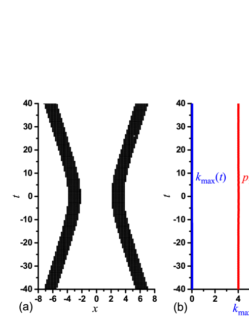
Figure 1: Collision of two kinks having velocities $V_{k}=\pm 0.1$ according to Eq. (9). (a) Trajectories of the soliton cores are shown by the regions where total energy density $e(x,t)>2$. (b) Maximal over spatial coordinate kinetic (blue) and potential (red) energy densities as the functions of time. Maximal energy density does not grow during collision of solitons having the same topological charge because they repel each other and their cores do not merge.

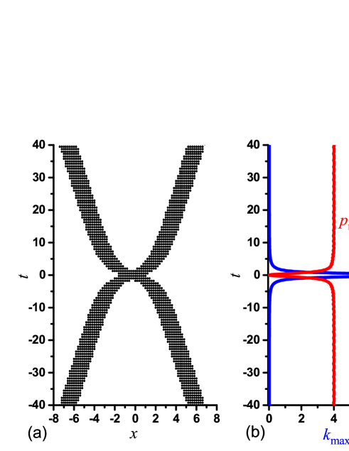
Figure 2: Same as in Fig. 1 but for the collision of a kink and an antikink given by Eq. (10) with subkink velocities $V_{k}=\pm 0.1$. Cores of the mutually attractive solitons merge at the collision point and total energy density at the collision point $e(x,0)=k(x,0)+p(x,0)$ rises up to about 8.

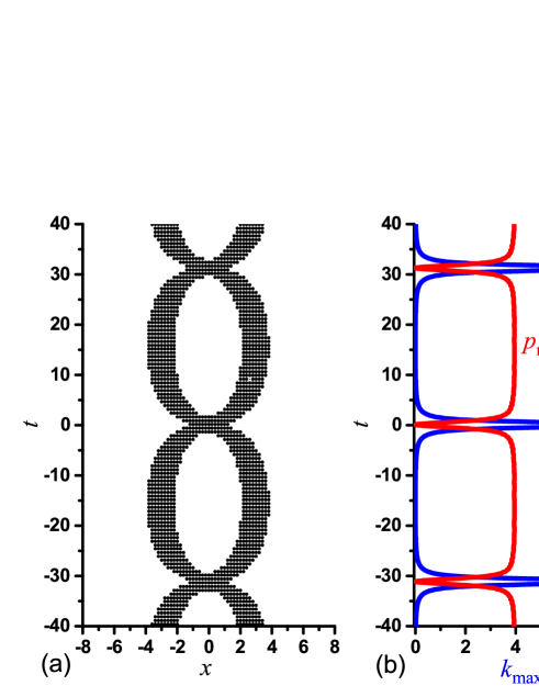
Figure 3: Same as in Fig. 1 but for the breather given by Eq. (7) with $V_{b}=0$ and $\omega=0.1$. When the subkinks collide, the potential energy density is almost zero and the kinetic energy density is about 8.

The two basic soliton solutions to SGE (1) are the kink (antikink)

$$\phi(x,t)=\pm 4\arctan\{\exp[\delta_{k}(x-V_{k}t)]\},$$ (6)

and the breather

$$\phi(x,t)=4\arctan\frac{\eta\sin[\delta_{b}\omega(t-V_{b}x)]}{\omega\cosh[\delta_{b}\eta(x-V_{b}t)]},$$ (7)

where $V_{k}$ is kink velocity, $V_{b}$, $\omega$ are the breather velocity and frequency, and

$$\delta_{k,b}=\frac{1}{\sqrt{1-V_{k,b}^{2}}},\quad\eta=\sqrt{1-\omega^{2}}.$$ (8)

The upper (lower) sign in Eq. (6) corresponds to the kink (antikink). The breather solution Eq. (7) can be regarded as a kink-antikink bound state Legrand ; Legrand1 ; CaputoFlytzanis .

A collision between two kinks having velocities $\pm V_{k}$ is described by the following solution to Eq. (1)

$$\phi(x,t)=4\arctan\frac{V_{k}\sinh(\delta_{k}x)}{\cosh(\delta_{k}V_{k}t)}.$$ (9)

For the collision between kink and antikink having velocities $\pm V_{k}$ one has the exact solution

$$\phi(x,t)=4\arctan\frac{V_{k}\cosh(\delta_{k}x)}{\sinh(\delta_{k}V_{k}t)}.$$ (10)

Substituting Eq. (6) and Eq. (7) into Eq. (2) one finds the total energies of the kink and breather

$$E_{k}=8\delta_{k},\quad E_{b}=16\delta_{k}\eta.$$ (11)

We are not interested in the relativistic effects and only slow solitons ($V_{k}\ll 1$, $V_{b}\ll 1$) will be considered so that $\delta_{k}\approx 1$ and $\delta_{b}\approx 1$. Only low-frequency breathers ($\omega\ll 1$) will be discussed so that $\eta\approx 1$. Then, we can write approximately that $E_{k}\approx 8$ and $E_{b}\approx 16$.

Even though the analytical expressions for multi-soliton solutions to SGE are available Backlund1 ; Backlund2 ; Hirota their complexity increases rapidly with the number of solitons, $N$. That is why for $N\geq 4$ we will do calculations numerically. For this we discretize Eq. (1) as follows

$$\frac{d^{2}\phi_{n}}{dt^{2}}-\frac{1}{h^{2}}(\phi_{n-1}-2\phi_{n}+\phi_{n+1})$$

$$+\frac{1}{12h^{2}}(\phi_{n-2}-4\phi_{n-1}+6\phi_{n}-4\phi_{n+1}+\phi_{n+2})$$

$$+\sin\phi_{n}=0,$$ (12)

where $h$ is the lattice spacing, $n=0,\pm 1,\pm 2,...$, and $\phi_{n}(t)=\phi(nh,t)$. To minimize the effect of discreteness, the term $\phi_{xx}$ in Eq. (1) is discretized with the accuracy $O(h^{4})$, which has been used previously BraunKivshar ; KivshMal ; Danial . The equations of motion in the form of Eq. (II) were integrated with respect to the time using an explicit scheme with the time step $\tau$ and the accuracy of $O(\tau^{4})$. The simulations reported in Sec. III were carried out for $h=0.1$, $h=0.05$ and $\tau=0.005$.

Before we start the presentation of the main results the following remark should be made. Two kinks (or two antikinks) repel each other as quasi-particles having the same topological charge. When they collide, they bounce off each other, their cores do not merge and, consequently, the maximal energy density does not grow. This is illustrated by Fig. 1, where for the solution Eq. (9) with $V_{k}=0.1$ we show (a) the regions of the $(x,t)$ plane where the total energy density $e(x,t)>2$ and (b) the maximal over $x$ densities of kinetic (blue line) and potential (red line) energies. The kinks collide at $t=0$, $x=0$. One can see that $k_{\max}(t)$ is nearly zero (due to the small kink velocity and the quadratic dependence on it), while $p_{\max}(t)\approx 4$, and these values are not affected by the collision.

On the contrary, kink and antikink are mutually attractive quasi-particles. Their cores merge during collision and the maximal energy density increases at the collision point. This can be seen in Fig. 2 where the kink-antikink solution Eq. (10) is presented for $V_{k}=0.1$. Far from the collision ($t=0$, $x=0$) we have $k_{\max}(t)\approx 0$ and $p_{\max}(t)\approx 4$. However, at $t=0$ $p_{\max}$ drops to zero, while $k_{\max}$ rises up to nearly 8, and so does the maximal total energy density $e_{\max}$ (not shown in the figure).

In Fig. 3 similar results are shown for the breather solution Eq. (7) with $V_{b}=0$ and $\omega=0.1$. It was already mentioned that the low-frequency breather can be envisioned as a kink-antikink bound state, and when the sub-kinks collide, $p_{\max}$ drops to zero and $k_{\max}$ reaches the value of nearly 8, as does $e_{\max}$. In the breather case, instead of this happening once (as in Fig. 2) the phenomenology periodically repeats itself, due to the time-periodicity of the state.

For the three-kink solutions it has been demonstrated that the cores of all three kinks can merge only if they collide in the spatial arrangement kink-antikink-kink (or antikink-kink-antikink) PREcollisions . This is understandable because in the combinations such as kink-kink-kink or kink-kink-antikink the solitons having the same topological charge repel each other because between them there is no a soliton of the opposite charge. In the following we will consider the multi-soliton solutions with alternating kinks and antikinks. In this case each kink (or antikink) attracts the nearest neighbors of the opposite charge and all of them can collide at one point, as it will be demonstrated in the following Section. This type of configurations promotes the energy exchange, contrary to what is the case for configurations bearing adjacent waves of the same type.

III Maximal energy density of multi-soliton solutions to the SGE

III.1 Case $N=1$

For a standing kink, Eq. (6) with $V_{k}=0$, the kinetic energy is zero. Then, the total energy density can be found from Eqs. (4)–(5) in the form

$$e(x)=p(x)=8\left(\frac{e^{x}}{1+e^{2x}}\right)^{2}+1-\cos(4\arctan e^{x}).$$ (13)

This function has maximum at $x=0$, which is the coordinate of the kink’s center. The value of the maximal energy density of the standing kink is

$$e^{(1)}_{\max}=p^{(1)}_{\max}=4.$$ (14)

III.2 Case $N=2$

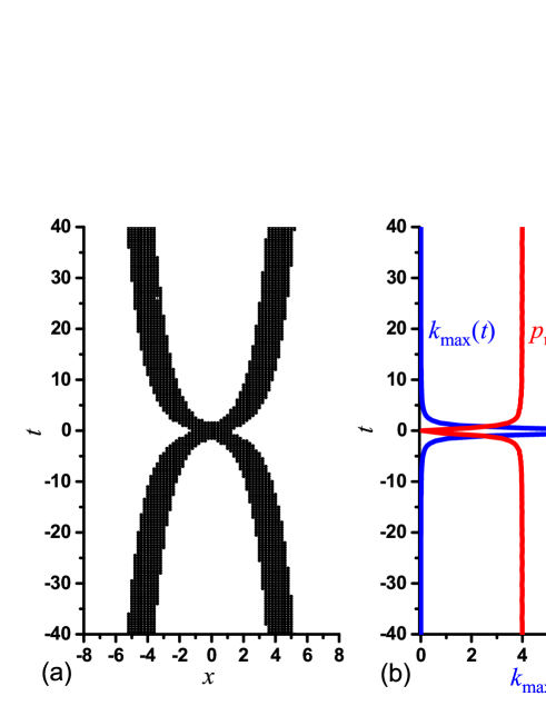
Figure 4: Same as in Fig. 1 but for the separatrix two-soliton solution of Eq. (15). When the kink and antikink collide the potential energy density is equal to zero and kinetic energy density is exactly 8.

The breather solution (7) for $V_{b}=0$ in the limit $\omega\rightarrow 0$, and the kink-antikink solution (10) in the limit $V_{k}\rightarrow 0$ both approach the same separatrix two-soliton solution

$$\phi(x,t)=4\arctan\frac{t}{\cosh x}.$$ (15)

This solution describes the kink and antikink that after the collision at $t=0$ move apart and their velocities vanish as $t\rightarrow\infty$. The solution is depicted in Fig. 4 where, as before, in (a) the points of the $(x,t)$ plane with $e(x,t)>2$ are shown and in (b) the maximal – over the spatial coordinate $x$ – values of kinetic (blue) and potential (red) energy densities are presented as functions of time. We now calculate the exact value of the maximal energy density by substituting Eq. (15) into Eqs. (4)–(5). The calculation can be simplified by noting that at $t=0$ one has $\phi(x,0)\equiv 0$ and thus, at the collision point the energy of the kink-antikink pair is in the form of kinetic energy,

$$e(x,0)=k(x,0)=\frac{8}{\cosh^{2}x}.$$ (16)

The energy density has maximum at the collision point $x=0$:

$$e^{(2)}_{\max}=k^{(2)}_{\max}=8.$$ (17)

III.3 Case $N=3$

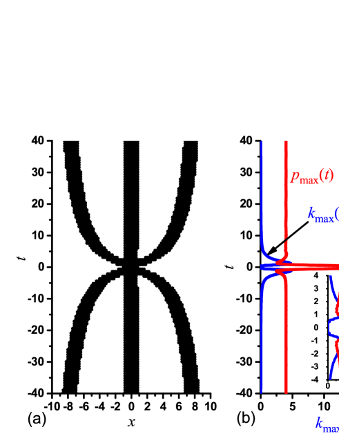
Figure 5: Same as in Fig. 1 but for the separatrix three-soliton solution Eq. (19). The inset shows the blowup of the region around $t=0$. When the two kinks collide with the antikink, the kinetic energy density is equal to zero and the potential energy density is exactly 20.

The kink-breather (3-soliton) solution to SGE reads

$$\phi(x,t)=4\arctan(\exp B)+4\arctan\frac{\eta Y}{\omega Z},$$

$$Y=2\omega(\sinh D-\cos C\sinh B)$$

$$+2\delta_{b}\delta_{k}(V_{k}-V_{b})\sin C\cosh B,$$

$$Z=2\eta(\cos C+\sinh D\sinh B)$$

$$-2\delta_{b}\delta_{k}(1-V_{k}V_{b})\cosh D\cosh B,$$

$$B=\delta_{k}(x-V_{k}t),$$

$$C=-\omega\delta_{b}(t-V_{b}x),\quad D=\eta\delta_{b}(x-V_{b}t).$$ (18)

In the limit $V_{k}\rightarrow 0$, $V_{b}\rightarrow 0$, and $\omega\rightarrow 0$, this solution assumes the following form (see Eq. (26) of Ref. Mirosh )

$$\phi(x,t)=4\arctan e^{x}+4\arctan\frac{x\cosh x-t^{2}\sinh x}{t^{2}+\cosh^{2}x}.$$ (19)

This separatrix solution describes the antikink standing at $x=0$ and two kinks that after the collision with the antikink at $t=0$ move apart and their velocities vanish as $t\rightarrow 0$. The solution is presented in Fig. 5 using a visualization similar to the previous figures.

To calculate the exact value of the maximal energy density, we again substitute Eq. (19) into Eqs. (4)–(5). Note that at $t=0$ one has $\phi_{t}(x,0)\equiv 0$ and thus, at the collision point the energy of the kink-antikink-kink solution is in the form of potential energy,

$$e(x,0)=p(x,0)=$$

$$8\left(\frac{e^{x}}{1+e^{2x}}+\frac{\cosh x-x\sinh x}{\cosh^{2}x+x^{2}}\right)^{2}$$

$$+1-\cos\left(4\arctan e^{x}+4\arctan\frac{x}{\cosh x}\right).$$ (20)

The energy density has maximum at the collision point $x=0$:

$$e^{(3)}_{\max}=p^{(3)}_{\max}=20.$$ (21)

III.4 Case $N=4$

The solution to SGE that describes collision of two breathers (i.e., a 4-soliton solution) with velocities $V_{1}$, $V_{2}$ and frequencies $\omega_{1}$, $\omega_{2}$ is given by

$$\phi(x,t)=4\arctan(S)-4\arctan\frac{\eta_{2}(T\cosh B_{1}+\sin C_{1})}{\omega_{2}(\cosh B_{1}+T\sin C_{1})},$$

$$T=\varphi\frac{2\tau[(S-P)(1+SP)-Q^{2}S]-2\beta Q(1+S^{2})}{\varphi^{2}[(1+S)(1+SP)+Q^{2}S^{2}]+(\tau^{2}+\beta^{2})[(S-P)^{2}+Q^{2}]},$$

$$P=\frac{\beta X+\kappa Y}{\varepsilon Z},\quad Q=\frac{\beta Y-\kappa X}{\varepsilon Z},\quad S=\frac{\eta_{1}\sin C_{1}}{\cosh B_{1}\omega_{1}},$$

$$X=\sinh B_{2}\cos C_{1}-\cos C_{2}\sinh B_{1},\,\,Y=\cosh B_{2}\sin C_{1}+\sin C_{2}\cosh B_{1},$$

$$Z=\cos(C_{1}-C_{2})+\cosh(B_{1}+B_{2}),$$

$$B_{1,2}=\eta_{1,2}\delta_{1,2}(x-x_{1,2}-V_{1,2}t),\,\,C_{1,2}=\Delta_{1,2}-\omega_{1,2}\delta_{1,2}[t-(x-x_{1,2})V_{1,2}],$$

$$\delta_{1,2}=(1-V_{1,2}^{2})^{-1/2},\,\,\eta_{1,2}=(1-\omega_{1,2}^{2})^{1/2},\quad\alpha=\frac{\delta_{2}(1+V_{2})}{\delta_{1}(1+V_{1})},$$

$$\beta=\alpha-1/\alpha,\quad\varepsilon=2\alpha-\beta+2(\omega_{1}\omega_{2}-\eta_{1}\eta_{2}),\quad\tau=2(\omega_{1}\eta_{2}-\eta_{1}\omega_{2}),\,\,$$

$$\varphi=2\alpha-\beta-2(\omega_{1}\omega_{2}+\eta_{1}\eta_{2}),\,\,\,\kappa=2(\omega_{1}\eta_{2}+\eta_{1}\omega_{2}).\,\,\,\,\,\,\,\,\,\,\,\,$$ (22)

Here $x_{1,2}$ and $\Delta_{1,2}$ define initial positions and initial phases of the two breathers, respectively.

It is possible to derive the separatrix solution from Eq. (III.4) in the limits $V_{1,2}\rightarrow 0$ and $\omega_{1,2}\rightarrow 0$ but the derivation is tedious and for $N>3$ we calculate the maximal energy density numerically considering collisions of slow kinks or slow, low-frequency breathers. Parameters of the colliding solitons are chosen to achieve collision of all $N$ subkinks at one point. Note that the collisions of two slow, low-frequency breathers were analyzed earlier in the study of fractal soliton collisions and the possibility for all four subkinks to collide at one point was demonstrated in Ref. PREfractal .

Equations (II) are integrated numerically for $h=0.1$, $h=0.05$ and $\tau=0.005$. Initial conditions are set with the help of Eq. (III.4). For simplicity, the collision of symmetric slow and low-frequency breathers is considered by setting $V_{1}=-V_{2}=0.1$, $\omega_{1,2}=0.1$, $\Delta_{1}=0$ and $\Delta_{2}=\pi$. To achieve the collision of all four subkinks at one point one should choose a proper initial distance between the breathers. In a series of numerical runs it is found that $x_{2}-x_{1}=4.012$ gives the desired result presented in Fig. 6.

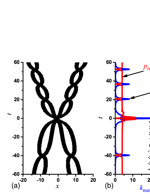
Figure 6: The result of the numerical simulation of the collision of two breathers (four subkinks). Initial conditions are set with the help of Eq. (III.4) with $V_{1}=-V_{2}=0.1$, $\omega_{1,2}=0.1$, $\Delta_{1}=0$ and $\Delta_{2}=\pi$, and $x_{2}-x_{1}=4.012$. (a) the soliton cores shown by the regions where $e(x,t)>2$. (b) Maximal –over the spatial coordinate $x$– kinetic (blue) and potential (red) energy densities as functions of time. The inset shows the curves near $t=0$. At the collision point potential energy density is practically zero, while the kinetic energy density increases up to nearly 32.

It can be seen in Fig. 6 that at the point of collision of the four subkinks the potential energy density is almost zero while the kinetic energy density shows a peak with a height nearly equal to 32. More precisely, for $h=0.1$ the largest energy density we could obtain by varying the parameter $x_{2}-x_{1}$ was 32.21, while for $h=0.05$ it was 32.05. With decreasing $h$ the accuracy of simulation increases. We thus conclude that the total energy density at the collision point is

$$e^{(4)}_{\max}=k^{(4)}_{\max}\approx 32.$$ (23)

Note that after the collision breathers have frequencies and velocities different from the initial values. This is due to the (weak but still nontrivial in this collision phenomenon) effect of discreteness, which breaks the integrability of the model. For more details on the inelasticity of near-separatrix multi-soliton collisions in weakly perturbed SGE see Refs. Mirosh ; PREfractal ; PREcollisions .

III.5 Case $N=5$

Here we set initial conditions using the individual kink (antikink) solution of Eq. (6) [rather than an extremely cumbersome 5-soliton solution]. As shown in Fig. 7(a), the initial positions and velocities of the five solitons are chosen such that initially they do not overlap and so that they collide at one point. As it was already mentioned, each soliton should attract its nearest neighbors and thus, it should have the topological charge opposite to that of its neighbors. In our case solitons 1, 3, and 5 are kinks and 2 and 4 are antikinks. The kink 3 is located at the origin and it is at rest, $x_{3}=0$ and $V_{3}=0$. The antikinks 2 and 4 have velocities $V_{2}=-V_{4}=0.025$ and initial positions $x_{2}=-x_{4}=-12.0$. By symmetry the solitons 2, 3, and 4 collide at one point. For the kinks 1 and 5 we take two times larger velocities $V_{1}=-V_{5}=0.05$ and choose their initial coordinates to achieve the collision of five solitons at one point. This happens for $x_{1}=-x_{5}=-24.376549$. Although the exactly coincident collision doesn’t happen for exactly double initial distances (from the origin) for double initial velocities, the latter is a reasonable rule of thumb for preparing the initial conditions of the multi-soliton configuration; a slight subsequent refinement may then be needed (such as the slight displacement of the outer kinks from $x_{1}=-x_{5}=24$ to $x_{1}=-x_{5}=-24.376549$).

As it can be seen from Fig. 7(b), when the five solitons collide, the maximal kinetic energy density is close to zero, while the maximal potential energy density is 50.93 for $h=0.1$ and 51.85 for $h=0.05$. We conclude that

$$e^{(5)}_{\max}=p^{(5)}_{\max}\approx 52.$$ (24)

A relevant additional remark here is that the significant role of weak asymmetries (in the preparation of our initial condition) can be observed to be exacerbated in the outcome of the collisional dynamics of Fig. 7. In particular, the figure showcases a visibly asymmetric result of the dynamics featuring, in addition to two outer nearly symmetric kinks, a breather (involving the anti-kink of soliton 2 and the kink of soliton 3) and a “stray” kink (the antikink of soliton 4). Once again here, the non-integrability of the underlying numerical scheme is deemed to be responsible for the observed asymmetry, although the energy density accumulation at $x=t=0$ is expected to persist even for an integrable discretization.

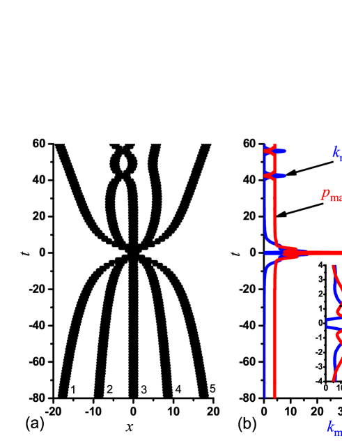
Figure 7: Collision of five kinks/antikinks at one point. The choice of initial conditions is described in the text. As before, in (a) the regions of the $(x,t)$ plane with energy density $e(x,t)>2$ are shown. In (b) the maximal, over $x$, kinetic and potential energy densities are shown as functions of time by the blue and red lines, respectively. At the collision point the potential energy density features the maximum of about approximately 52, while the kinetic energy density is almost zero. The inset shows the details of the curves near $t=0$. Note that the solitons are numbered in (a) before the collision. Odd quasi-particles are kinks and even ones are antikinks.

III.6 Case $N=6$

Referring to Fig. 8(a), note that the solitons 1, 3, and 5 are kinks and 2, 4, and 6 are antikinks. Initial soliton positions and velocities to achieve their collision at one point are: $x_{1}=-x_{6}=-34.90395$, $V_{1}=-V_{6}=0.1$, $x_{2}=-x_{5}=19.37864$, $V_{2}=-V_{5}=0.05$, $x_{3}=-x_{4}=-7$, $V_{3}=-V_{4}=0.025$. Once again, the velocities have been selected using factors of $2$, while the positions have been refined (from the corresponding factors of $2$) to ensure that the collision occurs for all solitons at the same point.

From Fig. 8(b) it is clear that at the collision point the maximal, over $x$, potential energy density is nearly zero while the maximal kinetic energy density reaches its highest attainable value. The height of the maximum is 72.62 for $h=0.1$ and 72.08 for $h=0.05$. Thus,

$$e^{(6)}_{\max}=k^{(6)}_{\max}\approx 72.$$ (25)

Here, solitons 2 and 3, as well as 4 and 5 merge in the symmetric aftermath of the collision into breather states (a feature that once again would be avoided in the realm of fully integrable dynamics).

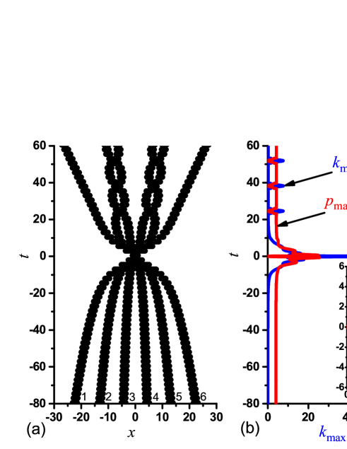
Figure 8: Same as in Fig. 7 but for the six-soliton collision. Initial conditions ensure the collision of all six kinks/antikinks at one point (see the text for the details). When the kinetic energy density reaches the maximal value of about 72, the potential energy density is almost zero.

III.7 Case $N=7$

In the initial configuration, odd solitons in Fig. 9(a) are the kinks and even are the antikinks. They collide at one point provided that their initial coordinates and velocities are chosen as follows: $x_{1}=-x_{7}=-39.541867403$, $V_{1}=-V_{7}=0.1$, $x_{2}=-x_{6}=-24.29923$, $V_{2}=-V_{6}=0.05$, $x_{3}=-x_{5}=-12$, $V_{3}=-V_{5}=0.025$, and $x_{4}=0$, $V_{4}=0$. Looking at Fig. 9(b) we note that at the collision point the maximal over $x$ kinetic energy density is extremely small, while the maximal potential energy density features a maximum of 94.90 for $h=0.1$ and 99.56 for $h=0.05$. It can then be stated that

$$e^{(7)}_{\max}=p^{(7)}_{\max}\approx 100.$$ (26)

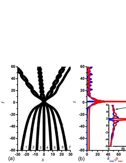
Figure 9: Same as in Fig. 7 but for the seven-soliton collision. All seven kinks/antikinks collide at one point due to proper choice of the initial conditions (see the text for the details). When the potential energy density reaches the maximal value of about 100, the kinetic energy density is almost zero.

The case of Fig. 9 is once again one of a pronounced asymmetric outcome, as we have generally observed odd $N$ cases to be (cf. Fig. 7). Three breathers are observed to form (solitons 2-3, 4-5, and 6-7), while the 1st soliton moves to the right in an isolated trajectory.

IV Conclusions & Future Challenges

In this work, we have provided a systematic calculation of the maximal energy density in the collision of $N$ slow kinks/antikinks (with $N\leq 7$) in the integrable sine-Gordon model. Our findings are collected in Table 1. The first line gives the number of colliding solitons, $N$. The second line gives the exact values of the maximal energy density that can be achieved in the collision of $N$ kinks/antikinks. These results are available for $N\leq 3$ (see Secs. III.1, III.2, and III.3). For larger $N$ the results were obtained numerically and they are presented in the third and fourth lines of Table 1 for $h=0.1$ and $h=0.05$, respectively. In numerical simulations the kink/antikink velocities are small (no greater than 0.1) but not equal to zero at $t\rightarrow\pm\infty$. For decreasing $h$ and decreasing initial velocities of the colliding kinks/antikinks the numerical results converge to the integer numbers shown in the last two lines of Table 1.

Table 1: Summary on maximal energy density in collision of $N$ solitons for $N\leq 7$.

$N$	0	$1$	$2$	$3$	$4$	$5$	$6$	$7$
Exact	0	$4$	$8$	$20$	$-$	$-$	$-$	$-$
$h=0.1$					$32.21$	$50.93$	$72.62$	$94.90$
$h=0.05$					$32.05$	$51.85$	$72.08$	$99.56$
$2N^{2}$	$0$	$-$	$8$	$-$	$32$	$-$	$72$	$-$
$2(N^{2}+1)$	$-$	$4$	$-$	$20$	$-$	$52$	$-$	$100$

The results can be summarized as follows. The maximal energy density that can be achieved in collision of $N$ slow kinks/antikinks in SGE is found to be equal to

$$e_{\max}^{(N)}\approx 2N^{2}\quad {\rm for\,\,even}\,\,N,$$

$$e_{\max}^{(N)}\approx 2(N^{2}+1)\quad {\rm for\,\,odd}\,\,N.$$ (27)

When an even number of slow kinks/antikinks collides at one point, the kinetic energy density reaches a maximal value $2N^{2}$, while the maximal potential energy density is nearly equal to zero. On the contrary, when an odd number of slow kinks/antikinks collides at one point, the potential energy density has maximal value $2(N^{2}+1)$, while the maximal kinetic energy density is almost zero.

These maximal energy density values can be achieved when all $N$ kinks/antikinks collide at one point. This happens when the kinks and antikinks approach the collision point alternatively (i.e., no two adjacent solitons are of the same type). Arranged in this way, each soliton has nearest neighbors of the opposite topological charge. Such solitons attract each other and their cores can merge producing a controllably high energy density spot, as we have demonstrated herein.

According to Eq. (IV), the maximal energy density in the sine-Gordon field that can be realized in $N$-soliton collisions increases quadratically with $N$. At the same time, total energy of $N$ standing kinks is equal to $8N$ and thus, is proportional to $N$. Naturally, this does not lead to a contradiction since the very high energy density is accumulated at a very narrow region near $x=0$, and hence when integrated over space, still preserves the total energy of $8N$. Furthermore, this very high concentration of energy density for a very short time interval (around $t=0$) is reminiscent of rogue events in other models (such as the nonlinear Schrödinger equation and variants thereof, with their Peregrine soliton and related solutions) pelin ; yan . However, to the best of our knowledge, no explicit rogue waveforms have been identified yet in such models. Hence, our identification of controllably large energy densities in the SGE model is, arguably, the first example of such a rogue event in this setting.

Having the results of this work in mind, one can expect that in the soliton gas model Baryakhtar ; Baryakhtar1 unlimited energy density can be achieved. Of course, the probability of collision of $N$ alternating kinks and antikinks decreases rapidly with increasing $N$ (and even then, the probability of their concurrent collision is very low), but such rare events can have important consequences, when they do arise.

As for the open problems, it is important to calculate the maximal energy density that can be achieved in multi-soliton collisions in other integrable and non-integrable systems of different dimensionality. For example, one can examine similar issues and design such collisions in other Klein-Gordon field theoretic models (e.g. in the $\phi^{4}$ or $\phi^{6}$ models Backlund1 ; Gani ), as well as in the one-dimensional, self-defocusing nonlinear Schrödinger equation. It would be particularly interesting to explore if the relevant phenomenology persists therein. It would also be particularly interesting to explore to attempt to prove the asymptotic statements inferred herein; although perhaps a direct approach towards this starting from a multi-soliton solution could be very cumbersome, perhaps a reverse approach, initializing the system with a suitably large, and highly localized energy density at a point and utilizing the inverse scattering transform to establish that this waveform will split into $N$ soliton solutions may be more tractable.

References

- (1) A.C. Scott, Am. J. Phys. 37, 52 (1969).
- (2) J. Cuevas-Maraver, P.G. Kevrekidis, and F. Williams, eds., The sine-Gordon Model and its Applications. From Pendula and Josephson Junctions to Gravity and High Energy Physics, Springer, Berlin, 2014.
- (3) L.P. Eisenhart, A treatise on the differential geometry of curves and surfaces, Ginn and Co., Boston, 1909.
- (4) S. Watanabe, H.S.J. van der Zant, S.H. Strogatz, T.P. Orlando, Physica D 97, 429 (1996).
- (5) J.K. Perring, T.H.R. Skyrme, Nucl. Phys. 31, 550 (1962).
- (6) S. Coleman, Phys. Rev. D 11, 2088 (1975).
- (7) O.M. Braun, Yu.S. Kivshar, The Frenkel-Kontorova Model: Concepts, Methods, and Applications (Springer, Berlin, 2004).
- (8) E.G. Ekomasov, R.R. Murtazin, O.B. Bogomazova, A.M. Gumerov, J. Magn. Magn. Mater. 339, 133 (2013).
- (9) S.V. Dmitriev, K. Abe, T. Shigenari, Physica D 147, 122 (2000).
- (10) S.V. Dmitriev, K. Abe, T. Shigenari, J. Phys. Soc. Jpn 65, 3938 (1996).
- (11) P.G. Drazin, Solitons, in: London Mathematical Society Lecture Note Series, Vol. 85, Cambridge University Press, Cambridge, 1983.
- (12) A. Barone, F. Esposito, C.J. Magee, A.C. Scott, Riv. Nuovo Cimento 1, 227 (1971).
- (13) Yu. S. Kivshar and B.A. Malomed Rev. Mod. Phys. 61, 763 (1989).
- (14) B. Birnir, H.P. McKean and A. Weinstein, Comm. Pure Appl. Math. 47, 1043 (1994).
- (15) R.K. Dodd, J.C. Eilbeck, J.D. Gibbon, H.C. Morries, Solitons and Nonlinear Wave Equations (Academic Press, London, 1982).
- (16) A.P. Fordy, A historical introduction to solitons and Bäcklund transformations. In A.P. Fordy, J.C. Wood, eds, Harmonic Maps and Integrable Systems, (Vieweg, Wiesbaden, 1994), PP. 7-28.
- (17) R. Hirota, J. Phys. Soc. Jpn 33, 1459 (1972).
- (18) L.A. Ferreira, B. Piette, and W.J. Zakrzewski, Phys. Rev. E 77, 036613 (2008).
- (19) L. Benfatto, C. Castellani, and T. Giamarchi, Phys. Rev. Lett. 99, 207002 (2007).
- (20) Z. Bajnok, L. Palla, and G. Takacs, Nucl. Phys. B 644, 509 (2002); Z. Bajnok, C. Dunning, L. Palla, G. Takacs, and F. Wagner, Nucl. Phys. B 679, 521 (2004).
- (21) D. M. Hofman and J. M. Maldacena, J. Phys. A 39, 13095 (2006).
- (22) P. Salmi, M. Hindmarsh, Phys. Rev. D 85, 085033 (2012).
- (23) S.B. Gudnason, M. Nitta, Phys. Rev. D 90, 085007 (2014).
- (24) A. Slunyaev, I. Didenkulova, E. Pelinovsky, Cont. Phys. 52, 571 (2011); see also: C. Kharif, E. Pelinovsky and A. Slunyaev, Rogue Waves in the Ocean, Springer-Verlag (Berlin, 2009).
- (25) Z. Yan, J. Phys. Conf. Ser. 400, 012084 (2012).
- (26) O. Legrand, G. Reinisch, Phys. Lett. A 35, 3522 (1987).
- (27) O. Legrand, Phys. Lett. A 36, 5068 (1987).
- (28) J.G. Caputo, N. Flytzanis, Phys. Rev. A 44, 6219 (1991).
- (29) D. Saadatmand, S.V. Dmitriev, D.I. Borisov, P.G. Kevrekidis, Phys. Rev. E 90, 052902 (2014).
- (30) S.V. Dmitriev, P.G. Kevrekidis, Yu.S. Kivshar, Phys. Rev. E 78, 046604 (2008).
- (31) A.E. Miroshnichenko, S.V. Dmitriev, A.A. Vasiliev, T. Shigenari, Nonlinearity 13, 837 (2000).
- (32) S.V. Dmitriev, Yu.S. Kivshar, T. Shigenari, Phys. Rev. E 64, 056613 (2001).
- (33) I.V. Baryakhtar, V.G. Baryakhtar, E.N. Economou, Phys. Rev. E 60, 6645 (1999).
- (34) I.V. Baryakhtar, V.G. Baryakhtar, E.N. Economou, Phys. Lett. A 207, 67 (1995).
- (35) V.A. Gani, A.E. Kudryavtsev, and M.A. Lizunova, Phys. Rev. D 89, 125009 (2014).