Linking the performance of endurance runners to training and physiological effects via multi-resolution elastic net

Abstract

A multiplicative effects model is introduced for the identification of the factors that are influential to the performance of highly-trained endurance runners. The model extends the established power-law relationship between performance times and distances by taking into account the effect of the physiological status of the runners, and training effects extracted from GPS records collected over the course of a year. In order to incorporate information on the runners’ training into the model, the concept of the training distribution profile is introduced and its ability to capture the characteristics of the training session is discussed. The covariates that are relevant to runner performance as response are identified using a procedure termed multi-resolution elastic net. Multi-resolution elastic net allows the simultaneous identification of scalar covariates and of intervals on the domain of one or more functional covariates that are most influential for the response. The results identify a contiguous group of speed intervals between 5.3 to 5.7 m$\cdot$s^-1 as influential for the improvement of running performance and extend established relationships between physiological status and runner performance. Another outcome of multi-resolution elastic net is a predictive equation for performance based on the minimization of the mean squared prediction error on a test data set across resolutions.
Keywords: regularization, grouping effect, collinearity, training distribution profile, power law, wearable GPS devices

1 Introduction

Competitive runners focus upon training effectively in order to enhance their fitness and performance. Yet despite many advances in the scientific evaluation of responses to training, the prescription and effectiveness assessment of training programmes relies upon the intuition and experience of runners and their coaches.

The early attempts to model the effects of training on performance were pioneered by Banister et al. (1975) who proposed an impulse-response model (see, also, Busso 2003 for a more recent application of the Banister et al. 1975 methodology). Banister and colleagues quantified training impulse as a single model input using arbitrary units, where the response is modelled as a change in performance that varies according to the training input. However, runners cannot use this model to inform their training as it requires frequent performance trials that interfere with their training programme. Several fundamental issues have also been highlighted by Busso and Thomas (2006) and Jobson et al. (2009). Specifically, the model needs input training data to be aggregated according to an assumed biological or physiological model. This biological or physiological model provides an abstraction of the complex relation between training input and response but has never been validated for this purpose. Critically, the necessary data aggregation restricts the use of the model to evaluating only programmes comprised of identical training sessions. Ultimately, the limitations of the model are such that its derived parameter estimates are not generalizable beyond the training session or participant studied.

A superior approach to modelling training would be to characterise its effects on race performance, i.e. as the time to cover a specified race distance. The relationship between best race performances over varying race distances has been found to follow a standard exponential curve over a wide range of values. Kennelly (1906) was the first to illustrate that the power law is a very good fit to this relation by plotting world best performances for men running from 100 m to 100 km, with an average deviation of only 4.3%. The more recent studies of Katz and Katz (1999) and Savaglio and Carbone (2000) have also confirmed that a power law fits well the relationship of best running performance and race distance. These models, however, do not account for the effect that training or the physiological status of the runner has on their performance, and hence they are overly simplistic into describing how the performance of individual runners varies accordingly.

With recent developments in training technology runners can now use GPS devices to record their training and races with a level of accuracy and detail that was previously inconceivable. The capability to obtain large volumes of training data from runners presents the opportunity for new insights into the links between training and performance by removing the need to use the limited impulse response model and by extending well-established parametric relationships for performance. That is the primary aim of the present study. The present study investigates the effects of training and physiological factors on the performance of highly-trained runners’ competing in distances from 800 metres to marathon (endurance runners, for short). A secondary aim is to produce a predictive equation for race performance. The available data are from a year-long observational study of 14 endurance runners, which produced detailed GPS records of their training, their physiological status and their best performance in standardised field tests (Galbraith et al., 2014).

The contribution of the present work is two-fold. Firstly, a multiplicative effects model for the performance of endurance runners is constructed, which extends the well-studied power-law relationship between runners’ performance times and distances by also taking into account the physiological status of the runner and information on the runners’ training. Particularly, in order to capture information on the runners’ training, the concept of the training distribution profile is introduced. The resulting model involves performance as a scalar response, a group of associated scalar covariates and the training distribution profile, which is a functional covariate. In order to simultaneously identify the speed intervals on the domain of the training distribution profile and the scalar physiological covariates that are important for explaining performance, we introduce a procedure termed multi-resolution elastic net. Multi-resolution elastic net proceeds by combining the partitioning of the domain of functional covariates in an increasing number of intervals with the elastic net of Zou and Hastie (2005), and results in predictive equations that involve only interval summaries of the functional covariates. We argue that the usefulness of multi-resolution elastic net extends beyond the present study. The supplementary material provides a reproducible analysis of a popular data set in functional regression analysis using multi-resolution elastic net.

The structure of the manuscript is as follows. Section 2 provides a description of the available data, along with an overview of the protocols used for data collection, the performance assessments and the collection of physiological status information from laboratory tests. Section 3 works towards setting up a general multiplicative effects model for performance that decomposes the performance times into effects due to race distance, physiological status, training and other effects. Section 4 describes multi-resolution elastic net and its use for estimating the parameters of the multiplicative model. The outcomes of the modelling exercise are described in Section 5 and confirm and extend established relationships between physiological status and runner performance, and, importantly, identify a contiguous group of speed intervals between 5.3 to 5.7 m$\cdot$s^-1 as influential for performance. A predictive equation for performance is also provided by the minimization of the estimated mean squared prediction error estimated from a test set across resolutions. The manuscript concludes with Section 6 which provides discussion and directions for further work.

2 Data

2.1 Participants

The available data were gathered as part of the study in (Galbraith et al., 2014) which examines changes in laboratory and field test running performances of highly-trained endurance runners. The study involved the observation of 14 competitive endurance runners, who had a minimum of 8 years experience of running training, and competition experience in race distances ranging from 800m to marathon. All participants provided written informed consent for this study which had local ethics committee approval from the University of Kent, Chatham Maritime, United Kingdom. More details on the participants, the study design and data collection protocols are provided in Galbraith et al. (2014), but a brief account is also provided below.

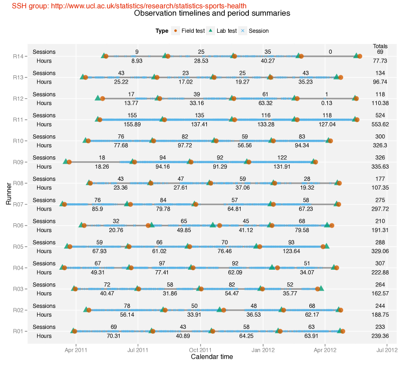
Figure 1: The observation timelines for the runners with the events of the study (lab tests, field tests and the recorded sessions for each runner) on a calendar scale. The number of recorded sessions and number of training hours within each training period and the corresponding totals are shown above, below and on the right of each timeline. In order to preserve anonymity the runners are referred to as R01, R02, $\ldots$, R14.

2.2 Data collection

The data was gathered by observing the training of the participating runners for a year. On commencing the study each runner was supplied with a wrist-worn GPS device (Forerunner^© 310XT, Garmin International Inc. Kansas, USA) and instructed in its use according to the manufacturer’s guidelines. The runners were asked to use the GPS device to record their training time and distance throughout every session and race in the observation period. The study did not involve any direct manipulation of the runners’ training programmes and the runners regularly downloaded the data from their GPS devices and sent the resulting files to the lead scientist.

In addition to their training, each runner completed 5 laboratory tests and 9 track-based field tests at regular intervals throughout the study. The laboratory tests were used to measure traditional physiological status determinants of running performance, i.e. running economy, OBLA (on-set blood lactate accumulation), and $\dot{V}O_{2max}$ (a measure of maximum oxygen consumption). The track-based field tests were conducted to measure the runners’ best performance over distances of $D_{1}=1200$ metres, $D_{2}=2400$ metres and $D_{3}=3600$ metres.

For the purposes of the current study, only the field tests that occurred within a few days of the laboratory tests are considered, i.e. 5 out of the 9 field tests for each runner. The complete observation period for each runner was set to the interval between and including the runner’s first and last field test.

Prior to all laboratory and field tests, careful standardisation ensured that each test was completed under conditions where the time of day, prior exercise, diet, hydration and warm up were specified and controlled. The runners were also familiarised with all laboratory and field tests before commencing the study.

2.3 Extraction of training sessions and speed profiles

The raw GPS data consists of 2,499,894 timestamped measurements of cumulative distances calculated using latitude and longitude information for the complete observation period for each runner. Those raw observations were used to identify 3,469 distinct training sessions accounting for 3,239.4 hours of recorded training activity. A technical note that details the process for extracting the training sessions from timestamped measurements is provided in the supplementary material. Figure 1 shows the resulting observation timeline for each runner and puts the events of the study on a calendar scale, where triangles denote lab tests, circles denote field tests and crosses denote training sessions. In what follows, a training period is defined as the interval between two consecutive field tests. So, as is also apparent from Figure 1, each runner had 4 training periods. The figure also shows the number of recorded sessions and number of training hours within each training period (above and below each timeline, respectively) and the corresponding totals for the whole timeline (on the right of each timeline). As seen on Figure 1, some runners have no training records for long intervals on their timelines. These intervals are either because of absence from training due to injury or vacation, or due to the runner failing to deliver their GPS container files to the scientist.

The training speed profiles for each training session shown in Figure 1 were calculated from the timestamped GPS measurements after appropriate imputation of zero speeds. The respective calculations and the imputation process are detailed in the technical note provided in the supplementary material.

3 Modelling running performance

3.1 An extended power law for running times

In order to investigate the effects of training and physiological factors on the running performance, it is assumed that the performance $Y_{ik}$ (in seconds) at the $i$th field test over distance $D_{k}$ decomposes as

$$Y_{ik}=\tau D_{k}^{\alpha}e^{\zeta_{i}}e^{\theta_{i}}e^{o_{i}}e^{\epsilon_{ik}}\quad(i=1,\ldots,56;k=1,\ldots,3)\,$$ (1)

where $\tau$ and $\alpha$ are the parameters controlling the power-law relationship between performance times and distances (Katz and Katz, 1999; Savaglio and Carbone, 2000) and $\epsilon_{ik}$ is an error component with zero mean. Model (1) extends the established power-law model for performance, by also taking into account the effect of the runners’ physiological status ($\zeta_{i}\in\Re$), the effect of training ($\theta_{i}\in\Re$), and the effects of other factors, for example psychological, environmental ($o_{i}\in\Re$) that can potentially influence performance. Model (1) asserts that the mean performance of the runners decomposes into a distance effect $D_{k}^{\alpha}$, a physiological status effect $e^{\zeta_{i}}$, a training effect $e^{\theta_{i}}$ and the effect $e^{o_{i}}$ of other unmeasured factors. Note that the inclusion of physiological status effects also brings runner-specific effects into the model.

In the current study we only have information for the distance, and the effects of physiological status effect and training. For this reason and taking into account the careful standardization prior to all laboratory and field tests (see Subsection 2.2 for more details), we assume that the effect of other unobserved factors on the performance across field tests is constant and set $e^{o_{i}}=1$.

Effect	Parameter	Covariate information
Distance ($\alpha\log D_{k}$)	$\alpha$	Distance (metres) for performance trial
Physiological status ($\zeta_{i}$)	$\gamma_{1}$	Weight (kg)
	$\gamma_{2}$	Height (cm)
	$\gamma_{3}$	Age (years)
	$\gamma_{4}$	$\dot{V}$O2max (ml$\cdot$min${}^{-1}\cdot$kg-1)
	$\gamma_{5}$	$\dot{V}$O2max (km$\cdot$h-1)
	$\gamma_{6}$	Economy (ml$\cdot$kg${}^{-1}\cdot$km-1)
	$\gamma_{7}$	Economy (kcal$\cdot$kg${}^{-1}\cdot$km-1)
	$\gamma_{8}$	OBLA (m$\cdot$s-1 at which blood lactate reaches 4mM)
Training ($\theta_{i}$)	$\delta_{0}$	Average session length (seconds)
	$\delta(s)$	Observed training distribution profile (seconds)

Table 1: The available covariate information that is used to characterize each of the effects in model (1).

3.2 Definition of physiological status effect

The physiological status effect in model (1) is assumed to have the additive form

$$\zeta_{i}=\gamma^{T}l_{i}\,,$$ (2)

where $\gamma$ is a vector of unknown parameters and $l_{i}$ is the vector of the laboratory test results at the end of the $i$th training period. Table 1 lists the available laboratory test results, which involve measurements on weight, height, age and physiological status determinants of running performance.

3.3 Definition of the training effect via training distribution profiles

3.3.1 Training distribution profiles

The definition of the training effect in model (1) has to incorporate an effective summary of the training that took place over each training period. Using directly some summary of the training speeds, such as a few quantiles, is an option but the speed profiles are rather noisy sometimes resulting in extreme speeds (see, for example, the top row of Figure 2 for two well-behaved profiles). So, the use of a smoothing procedure is necessary prior to the calculation of any summaries. This, though, would require assumptions on the behaviour of runners’ speeds during their regular training sessions as a function of time in order to determine the right amount of smoothing. Furthermore, any scalar summary of speeds over the training period does not directly reflect how the runner planned the allocation of speeds in the sessions within each training period.

In order to overcome such difficulties in defining the training effect, we introduce the concept of the training distribution profile. For a session $u$ that lasted $t_{u}$ seconds, let $K_{v}=\left\{t\,|\,\upsilon_{u}(t)>v\,,t\in(0,t_{u})\right\}$ and

$$\Pi_{u}(v)=\int_{0}^{t_{u}}I(\upsilon_{u}(t)>v)dt={\rm Length}(K_{v})\,.$$

We call the curve $\{v,\Pi_{u}(v)\,|\,v\geq 0\}$, the “training distribution profile”. The training distribution profile represents the training time spent exceeding any particular speed threshold and is a smoother representation of the allocation of speeds than the speed profile. Note that $\Pi_{u}(a)\geq 0$ for any $\alpha\geq 0$, and that $\Pi_{u}(a)=t_{u}$ for any $a<0$. In addition, $\Pi_{u}(v)$ is a necessarily decreasing function of speed.

The observed version of $\Pi_{u}(v)$ can be calculated using times and the calculated speeds (see the technical note in the supplementary material for details on the calculation of speeds) as

$$P_{u}(v)=\sum_{j=2}^{n_{u}}(T_{u,j}-T_{u,j-1})I(V_{u,j}>v)\,,$$ (3)

where $n_{u}$ is the number of observations after the imputation process has taken place, and $V_{u,j}$ is the calculated speed, in meters per second, at time $T_{u,j}$. Then, for a chosen grid $v_{1},\ldots,v_{k}$ of speed values, $\{v_{1},P_{u}(v_{1})\},\ldots,\{v_{k},P_{u}(v_{k})\}$, can be used to estimate the training distribution profile using smoothing techniques that respect the positivity and monotonicity of $\Pi_{u}(v)$. The top of Figure 2 shows two examples of speed profiles, one characteristic of an almost constant-pace training session and one from a high-intensity, interval-based training session. The corresponding estimated training distribution profiles are shown in the bottom row of Figure 2. As can be seen, the difference in the structure of the two training sessions alters the shape of the training distribution profiles correspondingly. The black curves in Figure 2 are calculated using (3) and the grey, smoother curves result from fitting a shape constrained additive model with Poisson responses (Pya and Wood, 2014) to ensure that the relationship between the smoothed version of $P_{u}(v)$ and $v$ is still monotone decreasing. The fitting is done using the scam package in R (R Core Team, 2015; Pya, 2014). Note that the resulting smoothed version is almost indistinguishable from $P_{u}(v)$ and from visual inspection (not reported here) this is the case for all recorded sessions in the data. For this reason, all subsequent analysis uses directly the smoothed versions.

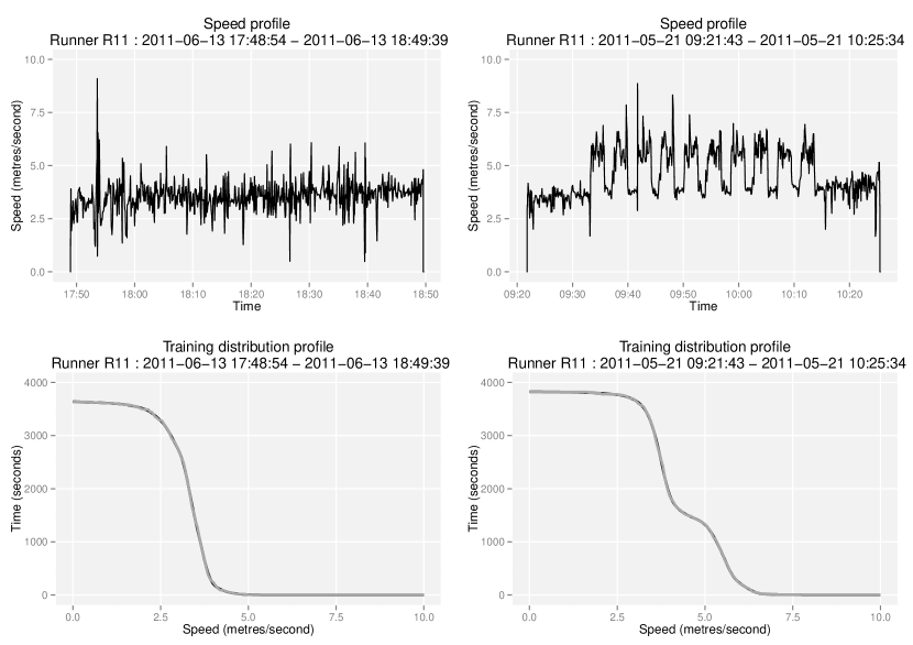
Figure 2: Two speed profiles (top) and the corresponding training distribution profiles (bottom). The black curves in are calculated using (3) and the grey smoother curves result by using a constrained shape additive model (Pya and Wood, 2014) with Poisson responses.

Any training sessions that correspond to estimated training distribution profiles with more than 125 seconds above 8 m$\cdot$s^-1 were dropped from the analysis as errors in data collection, because they exceed the world record speed for 800 metres (7.93 m$\cdot$s^-1 for 800m, David Rudisha, London Olympic Games, 9 August 2012). There were $18$ such sessions in the data and they have all been identified with the participants as bicycle rides or instances where the participants did not switch off their GPS device before driving their car or riding their bicycle after the end of training session.

3.3.2 Training effect

For defining the training effect in model 1, we assume that the average structure of the available training sessions within a training period (see Figure 1) approximates well the average training behaviour of runners for all the training sessions that took place in that period. We, further, assume that there is an unknown real-valued weight function $\delta(s)$, that weights the time spent at each speed according to its importance in determining performance.

$$\theta_{i}=\delta_{0}\bar{t}_{i}-\int_{0}^{\infty}\bar{P}^{\prime}_{i}(s)\delta(s)ds\quad(i=1,\ldots,56)\,,$$ (4)

where $\delta_{0}\in\Re$ is an unknown parameter and $\bar{P}^{\prime}_{i}(s)=d\bar{P}_{i}(s)/ds$ with $\bar{P}_{i}(s)$ being the average of the smoothed training distribution profiles for the $i$th training period. The quantity $\bar{t}_{i}=\bar{P}_{i}(-1)=\int_{0}^{\infty}\bar{P}^{\prime}_{i}(s)ds$ is the average session length in the $i$th period.

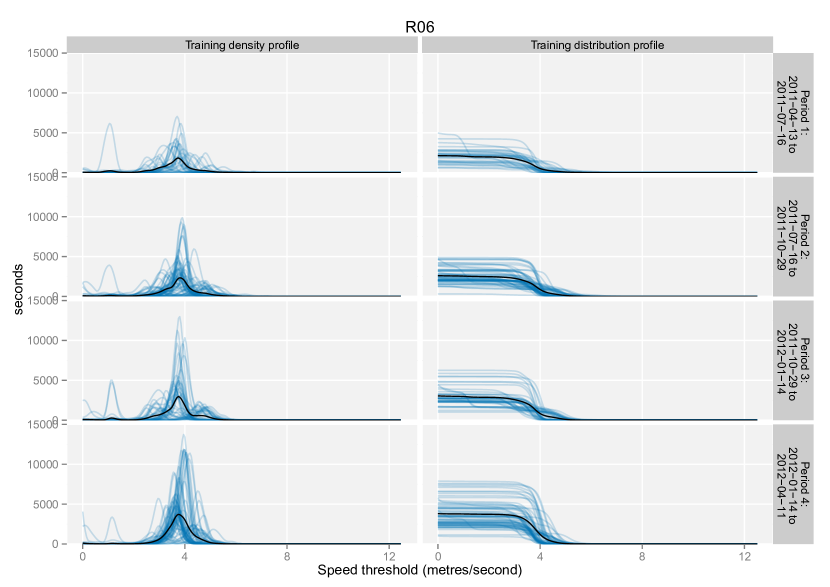
Figure 3: The observed, smoothed training distribution profiles for all sessions in the training periods for runner R06 (right) and their negative derivatives (left). The average curves are shown in black.

As a final note, in contrast to individual session speed profiles the concept of training distribution profiles appears well-suited for visualising large volumes of training session data. For example, the right panel of Figure 3 shows the estimated training distribution profiles for all sessions in the training periods of runner R06. The left panel shows the negative derivatives of those and reveals the clear concentration of training at around 4 m$\cdot$s^-1 which would have otherwise been hard to visualise. The average curves are shown in black.

4 Estimation

4.1 Multi-resolution elastic net

Table 1 lists the available covariate information that is used to characterize each of the effects in model (1). Taking logarithms on both sides, model (1) is a linear regression model with response the logarithm of the performance at the $k$th distance, $10$ scalar parameters (one for each scalar covariate in Table 1 and the intercept $\log\tau$) and a functional parameter $\delta(s)$.

We wish to be able to use that regression model to simultaneously assess the importance of scalar and functional covariates, also taking into account the correlation between the scalar covariates, and that between the scalar and the functional covariates. Particularly, the importance of the functional covariates can be assessed by identifying the training speed intervals that are important for performance changes. If there were no scalar covariates, one way to do so is the FLiRTI method in James et al. (2009), which induces sparseness simultaneously on $\delta(s)$ and on derivatives of it of a preset order.

In order to simultaneously identify important training speeds and important training covariates, we propose an alternative procedure which we term the multi-resolution elastic net and which consists of the following steps. For each resolution $G$ from a set of resolutions:

• Partition the union of the observed domains of the functional covariate across observations into $G$ intervals of the same length.

• Construct $G$ covariates by calculating a summary of the functional covariate for each observation and on each interval (e.g. integral, difference at endpoints and so on).

• Apply the elastic net (Zou and Hastie, 2005) on the covariates constructed in step b) along with any other available scalar covariates.

The $L_{2}$ penalty of the elastic net in step iii) controls for the extreme collinearity that the covariates of step ii) and any other scalar covariates can have, and the $L_{1}$ penalty of the elastic net imposes sparseness, if necessary. Note that the above makes no direct assumption on the ordering of the regression parameters corresponding to the functional covariate, as a functional regression approach would do. Instead, multi-resolution elastic net takes advantage of the grouping properties of the elastic net (Zou and Hastie, 2005, Section 2.3) for the formation of contiguous groups of non-zero estimates for the parameters of the highly correlated summaries of the functional covariates in step ii). In this way, if the non-zero elastic net coefficients of those parameters form contiguous groups, then there is strong evidence that the corresponding intervals are important for the response. A further persistence of those contiguous groups as the resolution $G$ increases will further strengthen any conclusions.

For the current application, in steps i) and ii) of the multi-resolution elastic net we replace (4) with the discretized version

$$\theta_{i}=\delta_{1}\bar{t}_{i}+\sum_{g=1}^{G}\left\{\bar{P}_{i}(v_{g-1})-\bar{P}_{i}(v_{g})\right\}\delta_{g}\quad(i=1,\ldots,56)\,,$$ (5)

where $\bar{P}_{i}(v_{g-1})-\bar{P}_{i}(v_{g})$ is the average training time spent in the $g$th speed interval before the $i$th end-of-period field test, and $\{v_{0},\ldots,v_{G}\}$ is an equi-spaced grid of speeds with $v_{0}=0$ and $v_{G}=12.5$ for some resolution $G=1,2,\ldots$. Then specification (5) and the scalar covariates are handled simultaneously in step iii) of the procedure. This last step will return estimates on $\beta=(\log\tau,\alpha,\gamma_{1},\ldots,\gamma_{8},\delta_{0},\delta_{1},\ldots,\delta_{G})^{T}$ and, hence, estimate the mean of the logarithmic performance

$$\log{\mu_{ik}(\beta;G)}=\log\tau+\alpha\log D_{k}+\gamma^{T}l_{i}+\delta_{0}\bar{t}_{i}+\sum_{g=1}^{G}\left\{\bar{P}_{i}(v_{g-1})-\bar{P}_{i}(v_{g})\right\}\delta_{g}\,,$$ (6)

for various resolutions $G$.

4.2 Selection of tuning constants and of optimal resolution

The above setup requires the determination of an optimal resolution $G$ for the training effects and the selection of the two tuning constants of the elastic net. In order to do so, the data set is first split into an estimation and a test set (the commonly used terminology for the “estimation set” is “training set” but we diverge from that in order avoid a terminology clash with the training effect $\theta_{i}$). Then, for each resolution, the tuning constants of the elastic net are selected as the ones that minimise the mean squared prediction error estimated using 10-fold cross-validation repeated for 10 randomly selected fold allocations in the estimation set. The selection of the two tuning constants of elastic net via cross-validation was implemented using the caret (Kuhn, 2008) and elasticnet (Zou and Hastie, 2012) R packages. The resolution $G$ is then determined as the one that minimises the mean squared prediction error estimated using the test set. Another outcome of this process is the estimated model for the chosen optimal resolution, which can be used for predictive purposes.

4.3 Estimation and test set

The six records that correspond to the last period for runners R12 and R14 were dropped from the data as uninformative because that period contained no or only one training records (see Figure 1). The resultant data set of 162 observations was then split into an estimation and test set. The test set is built from the records of 4 randomly selected runners. The reason for selecting amongst runners instead directly amongst records is to avoiding choosing an overoptimistic model in terms of prediction (note that the physiological status covariate information is repeated across distances in model (1)). The 114 records for the remaining 10 runners form the estimation set.

5 Results

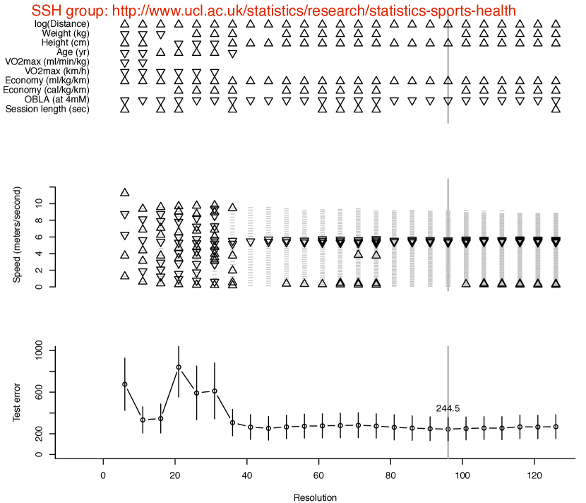
Figure 4: The non-zero estimated parameters for the chosen tuning constants of the elastic net for resolutions $G\in\{5,10,\ldots,125\}$. The vertical segments represent approximate normal-theory $95\%$ confidence intervals.

5.1 Distance and physiological status effects

Figure 4 shows the non-zero estimated parameters for the chosen tuning constants of the elastic net for resolutions $G\in\{5,10,\ldots,125\}$, where the maximal resolution of $125$ corresponds to speed intervals of length $0.1$ m$\cdot$s^-1 each. The figure provides a quick assessment of the relevance of each covariate. The symbols $\bigtriangledown$ and $\bigtriangleup$ in Figure 4 indicate negative and positive elastic net estimates respectively. The signs of the estimated parameters are all as expected.

As is apparent from the top plot in Figure 4 the distance of the field test, and the physiological status covariates of height (cm), running economy (ml$\cdot$kg${}^{-1}\cdot$km^-1) and running speed at OBLA are influential determinants of performance, irrespective of the resolution used. Particularly, the model indicates that without varying the training effects, shorter runners with higher speeds at OBLA and superior running economy (ml$\cdot$kg${}^{-1}\cdot$km^-1) perform better over a fixed race distance. The importance of each of OBLA, economy and height for running performance has been established and is consistent with previous study findings. For example, marathon performance has been shown to be predicted by running speed at OBLA and Sjödin and Jacobs (1981) suggest that OBLA is reflective of the underlying physiological status of endurance runners. The influence of running economy on endurance performance has been previous studied in Conley and Krahenbuhl (1980) for a cohort of highly-trained runners similar to those of the present study. In striking similarity to the current analysis, Conley and Krahenbuhl (1980) also found significant evidence that runners’ economy associates with performance whereas $\dot{V}O_{2max}$ is not. The relevance of height for endurance performance does not appear to have been widely studied. In this respect, Bale et al. (1986) examined a number of characteristics in a group of elite runners by dividing them according to by their best 10 kilometres performance time. They found significant evidence that the runners with larger performance times (slower) than the group’s median were taller than those who had run faster.

5.2 Training effects

The middle plot in Figure 4 indicates that the time spent training at speeds in the approximate interval from 5.3 to 5.7 m$\cdot$s^-1 is influential to the improvement in performance. The plot also shows that this result persists across all resolutions considered by the multi-resolution elastic net, and its importance is enhanced by the fact that within that interval and for all resolutions the non-zero estimates form a contiguous group. To the authors’ knowledge, this finding is the most specific to date in terms of analysing the contribution of training to subsequent performance.

Overall, the current analysis allows us to identify influential training speeds for subsequent performances within any training programme. This is in contrast to previous research where, typically, training speeds have been defined according to an underlying physiological model adopted prior to the commencement of the study, e.g. as percentages of the speed at $\dot{V}O_{2max}$ or OBLA. For example, Galbraith et al. (2014) identify 4.3 m$\cdot$s^-1 as the speed at OBLA, and then examine whether training at all speeds higher or lower than this links to changes in performance.

5.3 A predictive equation for performance

The records in the test set were used to calculate the squared prediction test error

$$\sum_{i\in\mathcal{T}}\sum_{k=1}^{3}\left(y_{ik}-\mu_{ik}(\hat{\beta};G)\right)^{2}$$

for each $G\in\{5,10,\ldots,125\}$, where $\mu_{ik}(\beta;G)$ is the exponential of (6) and $\mathcal{T}$ is the subset of $\{1,\ldots,162\}$ that contains the indices of the $48$ observations in the test set. The elastic net estimates $\hat{\beta}$ have been rescaled as in Zou and Hastie (2005) to avoid over-shrinkage due to the double penalization that takes place in elastic net. The test errors and the corresponding 95% normal theory intervals ($\pm$ 1.96 standard deviations) are shown at the bottom plot in Figure 4. The minimum test error is achieved for $G=95$.

Figure 5 shows the elastic net solution paths for that resolution as a function of the fraction of the $L_{1}$ norm. Particularly, the fit identified by the dashed line on the solution paths corresponds to the non-zero estimates at $G=95$ in Figure 4 (grey line). The elastic net estimates for the $G=95$ fit can be used to form the expression that predicts performance (in seconds) using the race distance, physiological status determinants as measured in the laboratory, and the average training distribution profile. This expression has been estimated to be

$$0.1310\text{``Distance (m)"}^{1.0568}$$ (7)

$$\exp\left\{0.1007\text{``Height (m)"}+0.1657\text{``Economy (L$\cdot$kg${}^{-1}\cdot$km${}^{-1}$)"}-0.0159\text{``OBLA (km$\cdot$h${}^{-1}$)"}\right\}$$

$$\exp\left\{-0.0078t_{1}-0.0279t_{2}-0.0307t_{3}\right\}\,,$$

where $t_{1},t_{2},t_{3}$ are the training period average times in minutes spent training within the speed intervals $(5.26,5.39]$, $(5.39,5.53]$, $(5.53,5.66]$, respectively. In order to reduce rounding error the units adopted in the above equation are rescaled from those in Table 1 so that height is calculated in metres and economy in litres per kilogram per kilometre. The exponent of Distance in (7) is in agreement with previous studies (Katz and Katz, 1999; Savaglio and Carbone, 2000) where it has been found to be around 1.1. Expression (7) can be used to determine the performance of an endurance runner for a specified race distance, by supplying the runner’s height, the measurement of economy and OBLA from a laboratory test prior to the race, and the average time spend training at the specified speed intervals during the period prior to the race.

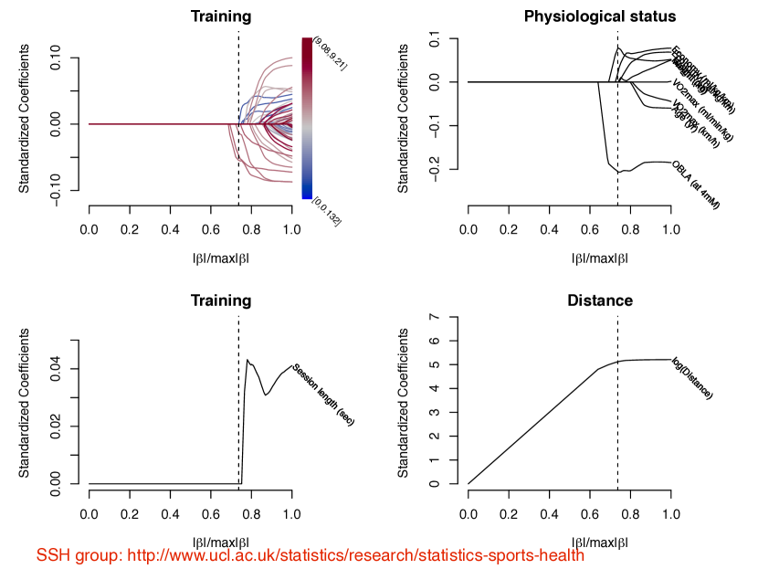
Figure 5: The elastic net solution paths for resolution $G=95$ versus the fraction of the $L_{1}$ norm. The fit identified by the dashed line on the solution paths corresponds to the non-zero estimates at $G=95$ in Figure 4.

6 Discussion

A multiplicative effects model has been used to link the training and physiological status of highly-trained endurance runners to their best performances. The model extends previous work that uses the power-law to describe the relationship between performance times and distance, by also including information on the physiological status of the runner as measured under laboratory conditions, and the runners’ training as extracted directly from GPS timestamped distance records for the period prior to the performance assessment.

The relevance of the training and physiology covariates in the model was assessed using multi-resolution elastic net, which is described in detail in Subsection 4.1. We argue that multi-resolution elastic net is a useful procedure to quickly check for the existence of influential intervals on the domain of one or more functional covariates in the presence of other scalar covariates. To provide some more evidence for our claim, a reproducible analysis of a popular dataset in functional regression is revisited in the supplementary material and the results of multi-resolution elastic net are sensible and in agreement with those of the FLiRTI procedure of James et al. (2009). Note that, the latter procedure is designed to handle regression models with only a single functional covariate. This is in contrast to multi-resolution elastic net that can simultaneously handle arbitrary number of scalar and functional covariates.

An important and novel aspect of the present study was to determine the direct effect of training on performance. Multi-resolution elastic net identified that the time spent training between 5.3 and 5.7 m$\cdot$s^-1 relates to improvements in the performance of the endurance runners. Another important aspect of the current study is that it was able to reproduce well-established relationships between performance and other physiological status measures (Conley and Krahenbuhl, 1980; Sjödin and Jacobs, 1981; Bale et al., 1986), without limitations posed by an underpinning physiological or training model. Specifically, it was found that without varying training effects, shorter runners with higher speeds at OBLA and superior running economy (ml$\cdot$kg${}^{-1}\cdot$km^-1) are found to perform better.

As mentioned in the Introduction section, the effect of training on performance has been modelled in studies like Banister et al. (1975) and Busso (2003) using a training impulse response model. The model adopted in those and similar studies, though, cannot be used for predictions beyond the training session and runner studied. Furthermore, the training inputs for the models in those studies are aggregated into arbitrary units thereby limiting their value to theoretical rather than practical applications. Indeed subsequently, Busso and Thomas (2006) stress the need for the development of new modelling strategies by stating that “it is likely that the expected accuracy between model prediction and actual data will greatly suffer from the simplifications made to aggregate total training strain in a single variable and, more generally, from the abstraction of complex physiological processes into a very small number of entities”. In this respect, expression (7) of our work generalises beyond the study design described in Section 2 and, in addition, it has been chosen as the best in terms of the predictive quality from the models arising from different levels of aggregation of the training inputs.

Training programmes and the individual sessions within them can be complex. This complexity can make it difficult to visualise and analyse a large training dataset without prior transformation or simplification. The current work contributes in this direction with the introduction of the concept of the training distribution profile. The training distribution profile promotes clear and straightforward visualisation of large volumes of training data (see for example Figure 3). More importantly, the training distribution profile allows the use of a wide range of contemporary statistical methods for the modelling of training data. For example, the training distribution profiles or their derivatives can directly be used as responses or covariates in functional regression models (see, for example Ramsay and Silverman, 2005, Chapters 15–17 for details) and/or for the detection of training regimes and changes in training practices, for example by a cluster analysis (James and Sugar, 2003). Furthermore, a more fruitful, if not more involved, analysis would, for example, take into account the variability of the training distribution profiles and/or their derivatives, as well as any serial correlation between them. The methods in Bathia et al. (2010) seem to provide a good basis in this direction. Given the widespread use of wearable data recording devices in training, distribution profiles of other aspects of a runner’s training can also be produced, such as heart rate distribution profiles and/or power-output profiles in cycling for example. Their influence on performance can then be determined using similar procedures as in the present study.

Overall, we try to reverse the prevailing scientific paradigm for investigating the effects of training on performance. Rather than evaluating the effects of a pre-specified training programme, we instead identify those aspects of training that link to a measurable effect. This presents an exciting and promising new approach to developing training theory. Importantly, the ability to identify important speeds presents an obvious focus for subsequent training interventions on the performance of endurance runners, and motivates further subject-specific work on the design and the study of the effectiveness of such interventions. If this work is successful, it has the potential to lead to the development of a new model of training which could be tuned towards maximising performance gains, or enhancing the health benefits arising from a prescribed amount of exercise.

7 Supplementary material

The supplementary material is appended at the end of the current preprint, and contains a reproducible analysis of the Canadian weather data (see, for example, James et al. 2009, Section 6 or Ramsay and Silverman 2005, Section 1.3) using multi-resolution elastic net and the FLiRTI procedure of James et al. (2009). The supplementary material also contains a technical note that details the process for extracting the training sessions and speed profiles from timestamped GPS measurements.

R scripts that reproduce the analyses undertaken in this manuscript are available upon request to the authors.

See pages 1,2,3,4 of runners_RSSC_supp_speeds.pdf See pages 1,2,3,4,5,6 of runners_RSSC_supp_Canadian_Weather.pdf

References

- Bale et al. (1986) Bale, P., D. Bradbury, and E. Colley (1986). Anthropometric and training variables related to 10km running performance. British Journal of Sports Medicine 20(4), 170–173.
- Banister et al. (1975) Banister, E. W., T. W. Calvert, M. V. Savage, and T. Bach (1975). A systems model of training for athletic performance. Australian Journal of Sports Medicine 7, 57–61.
- Bathia et al. (2010) Bathia, N., Q. Yao, and F. Ziegelmann (2010). Identifying the finite dimensionality of curve time series. The Annals of Statistics 38(6), pp. 3352–3386.
- Busso (2003) Busso, T. (2003). Variable dose-response relationship between exercise training and performance. Medicine and science in sports and exercise 35(7), 1188—1195.
- Busso and Thomas (2006) Busso, T. and L. Thomas (2006). Using mathematical modeling in training planning. International Journal of Sports Physiology & Performance 1(4), 400 – 405.
- Conley and Krahenbuhl (1980) Conley, D. L. and G. S. Krahenbuhl (1980). Running economy and distance running performance of highly trained athletes. Medicine and science in sports and exercise 12(5), 357–360.
- Galbraith et al. (2014) Galbraith, A., J. Hopker, M. Cardinale, B. Cunniffe, and L. Passfield (2014, March). A one-year study of endurance runners: Training, laboratory and field tests. International journal of sports physiology and performance.
- James and Sugar (2003) James, G. M. and C. A. Sugar (2003). Clustering for sparsely sampled functional data. Journal of the American Statistical Association 98(462), 397–408.
- James et al. (2009) James, G. M., J. Wang, and J. Zhu (2009). Functional linear regression that’s interpretable. The Annals of Statistics 37(5A), 2083–2108.
- Jobson et al. (2009) Jobson, S. A., L. Passfield, G. Atkinson, G. Barton, and P. Scarf (2009). The analysis and utilization of cycling training data. Sports Medicine 39(10), 833–844.
- Katz and Katz (1999) Katz, J. S. and L. Katz (1999). Power laws and athletic performance. Journal of Sports Sciences 17(6), 467–476.
- Kennelly (1906) Kennelly, A. E. (1906). An approximate law of fatigue in the speeds of racing animals. Proceedings of the American Academy of Arts and Sciences 42(15), pp. 275–331.
- Kuhn (2008) Kuhn, M. (2008, 11). Building predictive models in r using the caret package. Journal of Statistical Software 28(5), 1–26.
- Pya (2014) Pya, N. (2014). scam: Shape constrained additive models. R package version 1.1-7.
- Pya and Wood (2014) Pya, N. and S. Wood (2014). Shape constrained additive models. Statistics and Computing, to appear.
- R Core Team (2015) R Core Team (2015). R: A Language and Environment for Statistical Computing. Vienna, Austria: R Foundation for Statistical Computing.
- Ramsay and Silverman (2005) Ramsay, J. O. and B. W. Silverman (2005). Functional Data Analysis (2nd ed.). Springer.
- Savaglio and Carbone (2000) Savaglio, S. and V. Carbone (2000). Human performance: Scaling in athletic world records. Nature 404(6775), 244–244.
- Sjödin and Jacobs (1981) Sjödin, B. and I. Jacobs (1981). Onset of blood lactate accumulation and marathon running performance. International journal of sports medicine 2(01), 23–26.
- Zou and Hastie (2005) Zou, H. and T. Hastie (2005). Regularization and variable selection via the elastic net. Journal of the Royal Statistical Society: Series B (Statistical Methodology) 67(2), 301–320.
- Zou and Hastie (2012) Zou, H. and T. Hastie (2012). elasticnet: Elastic-Net for Sparse Estimation and Sparse PCA. R package version 1.1.