Fast Processing of SPARQL Queries on RDF Quadruples

Abstract

In this paper, we propose a new approach for fast processing of SPARQL queries on large RDF datasets containing RDF quadruples (or quads). Our approach called $\mathsf{RIQ}$ employs a decrease-and-conquer strategy: Rather than indexing the entire RDF dataset, $\mathsf{RIQ}$ identifies groups of similar RDF graphs and indexes each group separately. During query processing, $\mathsf{RIQ}$ uses a novel filtering index to first identify candidate groups that may contain matches for the query. On these candidates, it executes optimized queries using a conventional SPARQL processor to produce the final results. Our initial performance evaluation results are promising: Using a synthetic and a real dataset, each containing about 1.4 billion quads, we show that $\mathsf{RIQ}$ outperforms RDF-3X and Jena TDB on a variety of SPARQL queries.

1 Introduction

The Resource Description Framework (RDF) is a standard model for representing data on the Web [5]. It enables the interchange and machine processing of data by considering its semantics. While RDF was first proposed with the vision of enabling the Semantic Web, it has now become popular in domain-specific applications and the Web. Through advanced RDF technologies, one can perform semantic reasoning over data and extract knowledge in domains such as healthcare, biopharmaceuticals, defense, and intelligence. Linked Data [12] is a popular use case of RDF on the Web; it has a large collection of different knowledge bases, which are represented in RDF (e.g., DBpedia [10]).

With a growing number of new applications relying on Semantic Web technologies (e.g., Pfizer [4]; Newsweek, BBC, The New York Times, and Best Buy [1]) and the availability of large RDF datasets (e.g., Billion Triples Challenge (BTC) [6], Linking Open Government Data (LOGD) [2]), there is a need to advance the state-of-the-art in storing, indexing, and query processing of RDF datasets.

Today, datasets containing over a billion RDF quads are becoming popular on the Web (e.g., BTC [6], LOGD [2]). Such datasets can be viewed as a collection of RDF graphs. Using SPARQL’s GRAPH keyword [7], one can pose a query to match a specific graph pattern within any single RDF graph. While researchers in the database community have proposed scalable approaches for indexing and query processing of large RDF datasets [8, 28, 22, 9, 20, 13, 30, 31], they have designed these techniques for RDF datasets containing triples. In addition, none of them have investigated how large and complex graph patterns in SPARQL queries can be processed efficiently. Evidently, RDF-3X [22], a popular scalable approach for a local/centralized environment, yields poor performance when SPARQL queries containing large graph patterns are processed over large RDF datasets. This is because of the large number of join operations that must be performed to process a query.

We posit that, on RDF datasets containing billions of quads, any approach that first finds matches for subpatterns in a large graph pattern and then employs join operations to merge partial matches will face a similar limitation. Motivated by the aforementioned reasons, we propose a new approach called $\mathsf{RIQ}$ (RDF Indexing on Quads) and make the following contributions in this paper:

•  We propose a new vector representation for RDF graphs and graph patterns in SPARQL queries. This representation enables us to group similar RDF graphs and index each group separately rather than constructing an index on the entire dataset. We propose a novel filtering index, which employs a combination of Bloom Filters and Counting Bloom Filters to compactly store it.

•  We propose a decrease-and-conquer approach to efficiently process a SPARQL query. Using the filtering index, we can methodically and quickly identify candidate groups of RDF graphs that may contain a match for the query. We can then execute optimized queries on the candidates using a conventional SPARQL processor that supports quads.

•  We report the results from our initial performance evaluation using a synthetic and a real dataset, each containing about 1.4 billion quads. We observed that $\mathsf{RIQ}$ can outperform RDF-3X and Jena TDB on a variety of SPARQL queries.

2 Background

The RDF data model provides a simple way to represent any assertion as a (subject, predicate, object) triple. A collection of triples can be modeled as a directed, labeled graph. If each triple has a graph name (or context), it is called a quad. Below is an example of a quad from the BTC 2012 dataset [6] with its subject, predicate, object, and context: <http://data.linkedmdb.org/resource/producer/10138> <http://data.linkedmdb.org/resource/movie/producer_name> “Mani Ratnam" <http://data.linkedmdb.org/data/producer/10138>. Triples with the same context belong to the same RDF graph.

     PREFIX movie: <http://data.linkedmdb.org/resource/movie/>  PREFIX rdfs: <http://www.w3.org/2000/01/rdf-schema#>  PREFIX foaf: <http://xmlns.com/foaf/0.1/>  SELECT ?g ?producer ?name ?label ?page ?film WHERE {    GRAPH ?g { ?producer movie:producer_name ?name .               ?producer rdfs:label ?label .               OPTIONAL { ?producer foaf:page ?page . } .               ?film movie:producer ?producer .  } }     

Figure 1: An example of a SPARQL query

Using SPARQL, one can express complex graph pattern queries on RDF graphs. One of the fundamental operations in RDF query processing is Basic Graph Pattern Matching [7]. A Basic Graph Pattern (BGP) in a query combines a set of triple patterns. A triple pattern contains variables (prefixed by ?) and constants. During query processing, the variables in a BGP are bound to RDF terms in the data, i.e., the nodes in the same RDF graph, via subgraph matching [7]. Common variables within a BGP or across BGPs denote a join operation on the variable bindings of triple patterns. Consider the query shown in Figure 1. The bindings for the subject (variable) in ?producer movie:producer_name ?name are joined with the bindings for the object (variable) in ?film movie:producer ?producer. The variable ?g will be bound to the names/contexts of those RDF graphs that contain a match for the graph pattern specified inside the GRAPH block. OPTIONAL allows certain patterns to have empty bindings; UNION combines bindings of multiple graph patterns.

3 Related Work and Motivation

Several approaches have been developed for indexing and querying RDF data in a local/centralized environment. Early approaches employed an RDBMS to store and query RDF data (e.g., Sesame [16], Oracle [17]). Unfortunately, the cost of self-joins on a single (triples) table became a serious bottleneck. Later, Abadi et al.proposed the idea of vertically partitioning the property tables [29] and used a column-oriented DBMS to achieve an order of magnitude performance improvement over previous techniques [8]. Recently, Neumann et al.developed RDF-3X [22] that builds exhaustive indexes on the six permutations of $(s,p,o)$ triples. RDF-3X significantly outperformed the vertical partitioning approach. It uses a new join ordering method based on selectivity estimates and builds compressed indexes. Weiss et al. [28] developed Hexastore that also builds exhaustive indexes. However, Hexastore suffers from large index sizes due to lack of compression. Atre et al. [9] developed BitMat to overcome the overhead of large intermediate join results for queries containing low selectivity triple patterns. BitMat performs in-memory processing of compressed bit matrices during query processing.

More recently, Bornea et al. [13] developed DB2RDF by using an RDBMS to store and query RDF data. By storing the predicate-object pairs of each subject in the same row of the relational table, they reduced the number of joins required for star-shaped BGPs. DB2RDF maintains only subject and object indexes and employs a novel SPARQL-to-SQL translation technique for generating optimized queries. Yuan et al. [30] developed TripleBit, which uses a compact storage scheme for RDF data by representing triples via a Triple Matrix. For each predicate, TripleBit maintains SO and OS ordered buckets. Using a collection of indexes and optimal join ordering, it reduces the size of the intermediate results during query processing.

A few approaches exploit the graph properties/structure of RDF data for indexing and query processing [25, 27, 14, 32, 23]. These techniques, however, have been tested only on small RDF datasets containing less than 50 million triples. Recently, a few schemes were proposed for distributed/parallel RDF query processing [20, 31]. Our work, however, focuses on RDF query processing in a local environment.

The motivation for our work stems from two key observations: First, the above approaches were designed to process RDF datasets containing triples. Simply ignoring the context in an RDF quad and using an existing approach designed for triples may produce incorrect results due to bindings for a BGP from different graphs [26]. Second, most of the queries tested by these approaches contain BGPs with a modest number of triples patterns (at most 8). None of them have investigated how to efficiently process SPARQL queries with large, complex BGPs (e.g., containing undirected cycles).

4 The Design of $\mathsf{RIQ}$

     Query => ’SELECT’ Variables ’WHERE’ ’{’ ’GRAPH’ Variables    ’{’ GroupGraphPattern ’}’ ’}’ ResultModifiers  GroupGraphPattern => BGP? ( GraphPatternNotTriples ’.’? BGP? )*  GraphPatternNotTriples =>    GroupOrUnionGraphPattern | OptionalGraphPattern | Filter  GroupOrUnionGraphPattern =>    GroupGraphPattern ( ’UNION’ GroupGraphPattern )*  OptionalGraphPattern => ’OPTIONAL’ GroupGraphPattern  Filter => ’FILTER’ Constraint  Constraint => Predicate | ’EXISTS’ BGP | ’NOT EXISTS’ BGP     

Figure 2: Grammar for queries

In this section, we present the design of $\mathsf{RIQ}$ (RDF Indexing on Quadruples) and describe its three main components, i.e., the Indexing Engine, the Filtering Engine, and the Execution Engine. (See Figure 3.) Our goal is to support a subset of the SPARQL grammar [7] as shown in Figure 2.

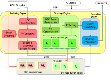
Figure 3: Overview of $\mathsf{RIQ}$

4.1 Indexing RDF Data

We introduce a new vector representation for RDF graphs and BGPs, which will allows us to capture the properties of the triples and triple patterns in them. This vector representation plays a key role in the construction of an effective filtering index, where similar RDF graphs will be grouped together.

4.1.1 Essential Transformations

To begin with, we define two transformations: one for a triple in an RDF graph and the other for a triple pattern in a BGP. Let $\mathbb{P}$ = {$SPO$, $SP?$, $S?O$, $?PO$, $S??$, $?P?$, $??O$} be a set of canonical patterns. We denote the transformation on a triple (s,p,o) by $f_{D}:\mathbb{P}\times\{(s,p,o)\}\rightarrow O_{D}$, where the range $O_{D}$ is shown Table 1 for each canonical pattern. Note that $O_{D}$ resembles triple patterns (variable names excluded) that can appear in a BGP.

Transformation $f_{D}$	Transformation $f_{Q}$
$f_{D}$(SPO, (s,p,o)) = (s,p,o)	$f_{Q}$(‘s p o’) = (SPO,(s,p,o))
$f_{D}$(SP?, (s,p,o)) = (s,p,?)	$f_{Q}$(‘s p ?$v_{o}$’) = (SP?,(s,p,?))
$f_{D}$(S?O, (s,p,o)) = (s,?,o)	$f_{Q}$(‘s ?$v_{p}$ o’) = (S?O,(s,?,o))
$f_{D}$(?PO, (s,p,o)) = (?,p,o)	$f_{Q}$(‘?$v_{s}$ p o’) = (?PO,(?,p,o))
$f_{D}$(S??, (s,p,o)) = (s,?,?)	$f_{Q}$(‘s ?$v_{p}$ ?o’) = (S??,(s,?,?))
$f_{D}$(?P?, (s,p,o)) = (?,p,?)	$f_{Q}$(‘?$v_{s}$ p ?$v_{o}$’) = (?P?,(?,p,?))
$f_{D}$(??O, (s,p,o)) = (?,?,o)	$f_{Q}$(‘?$v_{s}$ ?$v_{p}$ o’) = (??O,(?,?,o))

Table 1: Transformations in $\mathsf{RIQ}$

Next, we denote a transformation $f_{Q}:T\rightarrow\mathbb{P}\times O_{Q}$, where $T$ denotes the set of triple patterns that can appear in a query. The range $\mathbb{P}\times O_{Q}$ is shown in Table 1 and identifies the canonical pattern for a given triple pattern. Although the triple pattern ‘s p o’ has no variables, it is still a valid triple pattern in a BGP.

The transformations $f_{D}$ and $f_{Q}$ allow us to map a triple in the data and a triple pattern in a query to a common plane of reference. This will enable us to quickly test if a triple pattern in a BGP has a match in the data.

4.1.2 Pattern Vectors

Given an RDF graph with context $c$, we map it into a vector representation called a Pattern Vector (PV) and denote it by $\overline{V_{c}}$. Essentially, $\overline{V_{c}}$ = ($V_{c,SPO}$, $V_{c,SP?}$, $V_{c,S?O}$, $V_{c,?PO}$, $V_{c,S??}$, $V_{c,?P?}$, $V_{c,??O}$), where each $V_{c,r}$ denotes the vector constructed for $r\in\mathbb{P}$. We assume a hash function $\mathbb{H}:B\rightarrow\mathbb{Z}^{*}$, where $B$ denotes a bit string and the range is the set of non-negative integers. Now, we construct $\overline{V_{c}}$ as follows: Initially, each $V_{c,r}$ is empty. Given a quad $(s,p,o,c)$ in the graph, for each $r\in\mathbb{P}$, we compute $\mathbb{H}(f_{D}(r,(s,p,o)))$ and insert it into $V_{c,r}$. We perform this computation on every quad in the graph to generate $\overline{V_{c}}$. Note that $\overline{V_{c}}$ requires space linear in the number of quads in the graph.

Our hash function $\mathbb{H}$ is based on Rabin’s fingerprinting technique [24], which is efficient to compute. If we generate 32-bit hash values, the probability of collision is extremely low [26]. Thus, in practice, we can view $V_{c,SPO}$ as a set, because the quads/triples in a graph are always assumed to be unique. However, the remaining vectors of $\overline{V_{c}}$ should be viewed as multisets, because $f_{D}$ can produce the same output for different triples due to the presence of ‘?’ in the output.

Given a BGP $q$, we map it into a PV, denoted by $\overline{V_{q}}$, and compute it slightly differently: Initially, each $V_{q,r}$ is empty. For each triple pattern $t$ in $q$, we compute $f_{Q}(t)$ to produce a pair $(r,o)$, where $r$ denotes the canonical pattern for $t$. We then insert $\mathbb{H}(o)$ into $V_{q,r}$. As before, $V_{q,SPO}$ can be viewed as a set. The rest of the vectors of $\overline{V_{q}}$ should be viewed as multisets, because two different triple patterns (each containing at least one variable) in a BGP may hash to the same value. For example, if a BGP contains two triple patterns ?$s_{1}$ movie:producer ?$o_{1}$ and ?$s_{2}$ movie:producer ?$o_{2}$, then $f_{Q}$(‘$?s_{1}$ movie:producer $?o_{1}$’) = $f_{Q}$(‘$?s_{2}$ movie:producer $?o_{2}$’) and therefore, the hash values produced by $\mathbb{H}$ will be identical.

4.1.3 Operations on Pattern Vectors

Next, we define two operations on PVs, which will be used during the construction of the filtering index. Our goal is to group similar PVs (and as a result, similar RDF graphs) together so that candidate RDF graphs are identified and processed quickly during query processing.

Definition 1 (Union)

Given two PVs, say $\overline{V_{a}}$ and $\overline{V_{b}}$, their union $\overline{V_{a}}\cup\overline{V_{b}}$ is a PV say $\overline{V_{c}}$, where $V_{c,r}\leftarrow V_{a,r}\cup V_{b,r}$ and $r\in\mathbb{P}$.

Definition 2 (Similarity)

Given two PVs, say $\overline{V_{a}}$ and $\overline{V_{b}}$, their similarity is denoted by $sim(\overline{V_{a}},\overline{V_{b}})$ = $\max\limits_{r\in\mathbb{P}}$ $sim(V_{a,r},V_{b,r})$, where $sim(V_{a,r},V_{b,r})=\frac{|V_{a,r}\cap V_{b,r}|}{|V_{a,r}\cup V_{b,r}|}$.

4.1.4 Index Construction

We begin by describing a key necessary condition, which forms the basis for indexing and query processing in $\mathsf{RIQ}$. Because we map both the RDF graphs and BGPs into their PVs, we must characterize the relationship between them when processing a BGP – assuming it is a connected graph – via subgraph matching. We state the following theorem.

Theorem 1

Suppose $\overline{V_{c}}$ and $\overline{V_{q}}$ denote the PVs of an RDF graph and a BGP, respectively. If the BGP has a subgraph match in the RDF graph, then $\bigwedge\limits_{r\in\mathbb{P}}(V_{q,r}\subseteq V_{c,r})=$ TRUE. (See the technical report [26] for the proof.)

According to Theorem 1, given a BGP, if we can identify those RDF graphs in the database whose PVs satisfy the necessary condition, then we have a superset of RDF graphs that contain a subgraph match for the BGP. This also guarantees that there are no false dismissals.

Rather than testing every PV in the database – one-at-a-time – during query processing, we propose a novel filtering index called the PV-Index to effectively organize millions of PVs in the database. Using this index, we aim to quickly identify candidate RDF graphs in the early stages of query processing using Theorem 1. Our goal is to discard most of the non-matching RDF graphs without any false dismissals. As a result, the subsequent stages of query processing will process fewer candidates to obtain the final results, thereby speeding up query processing.

There are two issues that arise while designing the PV-Index: First, we want to group similar PVs together so that for a given BGP, we can quickly discard most of the non-matching RDF graphs. Second, we want to compactly store the PV-Index to minimize the cost of I/O during query processing. To address the first issue, we use the concept of locality sensitive hashing (LSH) [21]. For similarity on sets based on the Jaccard index, LSH on a set $S$, denoted by $\mathsf{LSH}_{k,l,m}(S)$ can be performed as follows [19]: Pick $k\times l$ random linear hash functions of the form $h(x)=(ax+b)~{}mod~{}u$, where $u$ is a prime, and $a$ and $b$ are integers such that $0<a<u$ and $0\leq b<u$. Compute $g(S)=\min\{h(x)\}$ over all items in the set as the output hash value for $S$. Each group of $l$ hash values is hashed (e.g., using Rabin’s fingerprinting) to the range $[0,m-1]$. This results in $k$ hash values for $S$. It is known that given two sets $S_{1}$ and $S_{2}$ with similarity $p=\frac{|S_{1}\cap S_{2}|}{|S_{1}\cup S_{2}|}$, $\Pr[g(S_{1})=g(S_{2})]=p$. Also, the probability that $\mathsf{LSH}_{k,l,m}(S_{1})$ and $\mathsf{LSH}_{k,l,m}(S_{2})$ have at least one hash value identical is $1-(1-p^{l})^{k}$. The above properties also hold for multisets.

To address the second issue, we employ Bloom filters (BFs) and Counting Bloom filters (CBFs) [15] to compactly represent the PV-Index. A Bloom filter is a popular data structure to compactly represent a set of items and process membership queries on it. A Counting Bloom filter maintains $n$-bit counters instead of single bits and can represent multisets. Both BFs and CBFs can be configured to achieve a false positive rate based on their capacities [15].

Algorithm 1 The PV-Index Construction

0:  a list of PVs; $(k,l,m)$: LSH parameters; $\epsilon$: false positive rate

0:  filters of all the groups of similar RDF graphs

1:  Let $\mathbb{G}(\mathbb{V},\mathbb{E})$ be initialized to an empty graph

2:  for each PV $\overline{V}$ do

3:     Add a new vertex $v_{i}$ to $\mathbb{V}$

4:     for each $r\in\mathbb{P}$ do

5:        $\{h_{i1},...,h_{ik}\}\leftarrow\mathsf{LSH}_{k,l,m}(V_{r})$

6:        for every $v_{j}\in\mathbb{V}$ and $i\neq j$ do

7:           if $\exists~{}o$ s.t. $1\leq o\leq k$ and $h_{io}=h_{jo}$ then

8:              Add an edge $(v_{i},v_{j})$ to $\mathbb{E}$ if not already present

9:  Compute the connected components of $\mathbb{G}$. Let $\{C_{1},...,C_{t}\}$ denote these components.

10:  for $i=1$ to $t$ do

11:     Compute the union $U_{i}$ of all PVs corresponding to the vertices in $C_{i}$

12:     Construct a BF for $U_{i,SPO}$ with false positive rate $\epsilon$ given the capacity $|U_{i,SPO}|$

13:     Construct a CBF for each of the remaining vectors of $U_{i}$ with false positive rate $\epsilon$ given the capacity $|U_{i,*}|$

14:     Store the ids of graphs belonging to $C_{i}$

15:  return  

In Algorithm 1, we outline the steps to construct the PV-Index. We build a graph $\mathbb{G}$, where each vertex of $\mathbb{G}$ represents a PV. For every PV, we apply LSH on each of its seven vectors. Suppose there are two PVs such that the application of LSH on their vectors for the same pattern $r$, produces at least one identical hash value, then we add an edge between the vertices representing these PVs (Lines 2 to 8). Essentially, a missing edge between two vertices indicates that their corresponding PVs are dissimilar with high probability. Once $\mathbb{G}$ is constructed, we compute (in linear time) the connected components in it. Each connected component represents RDF graphs whose corresponding PVs are similar with high probability. We treat these graphs as a group and compute the union of their PVs (Line 11). The union operation summarizes the PVs as well as preserves the condition stated in Theorem 1. (The individual vectors in a PV are sorted to enable the union operation in linear time.)

To compactly represent the union computed for a connected component, we use a combination of one Bloom filter (BF) and six Counting Bloom filters (CBFs). The vector for the canonical pattern SPO is stored using a BF and the others are stored using CBFs. Each filter of a vector is configured for a false positive rate of $\epsilon$ and capacity equal to the cardinality of the vector (Lines 12 and 13). For each connected component, we also store the ids of graphs belonging to it. In summary, the BFs and CBFs for all the connected components constitute the PV-Index. Each group of graphs is separately indexed using a tool like Jena TDB.

4.2 Query Processing

Next, we propose a decrease-and-conquer approach for efficient SPARQL query processing in $\mathsf{RIQ}$. That is, we first identify candidate groups of RDF graphs that may contain matches for a query using the PV-Index and then execute optimized SPARQL queries on these candidates.

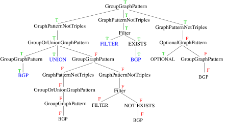
Figure 4: An example of a BGP Tree

Given a query, the first step is to parse its GRAPH block according to the grammar in Figure 2 and generate a tree-representation, which we call the BGP Tree. This tree serves as an execution plan for processing individual BGPs in the query. (See Figure 4 for an example.) We maintain a Boolean variable $eval[n]$ for each node $n$ in the tree to denote the status of the evaluation on a connected component of the PV-Index. With $eval[n]=$ FALSE for every node in the tree, we invoke Algorithm 2 on each connected component, starting from the root of the BGP Tree. When a child of GroupGraphPattern evaluates to FALSE, we skip processing the remaining children (Line 4), because the RDF graphs belonging to that connected component will not produce a match for the subexpression rooted at GroupGraphPattern. For GroupOrUnionGraphPattern, however, at least one of its children i.e., GroupGraphPattern, should evaluate to TRUE to produce a match (Line 7).

When a BGP is encountered (Line 15), we test the necessary condition stated in Theorem 1 by calling Algorithm 3. This involves the processing of membership queries on the BF and CBFs constructed for that connected component. If OptionalGraphPattern evaluates to FALSE, we return TRUE because of the semantics of OPTIONAL in SPARQL. If $eval[root]$ = TRUE, then the group of RDF graphs belonging to that connected component is a candidate for further processing.

For the candidate, an optimized SPARQL query can be generated by traversing the BGP Tree and checking the evaluation status of each node. (In the interest of space, we provide the algorithm in the technical report [26].)

The result modifiers and predicates within FILTER are included in the optimized query. In Figure 4, we show an example, where the OPTIONAL block and one block in the UNION will be discarded in the optimized query. The optimized query can then be executed on the candidate using a tool like Jena TDB. The results from all the candidates should be combined to produce the final results.

Algorithm 2 EvalBGPTree(node $n$, conn. component $j$)

1:  Let $c_{1},...,c_{\tau}$ denote the child nodes of $n$ (left-to-right)

2:  for $i$ = $1$ to $\tau$ do

3:     $eval[c_{i}]$ $\leftarrow$ EvalBGPTree($c_{i}$, $j$)

4:     if $n$ is GroupGraphPattern & $eval[c_{i}]$ = FALSE then

5:        $eval[n]$ $\leftarrow$ FALSE

6:        return  FALSE {//skip rest of the nodes}

7:  if $n$ is GroupOrUnionGraphPattern then

8:     $eval[n]\leftarrow\bigvee\limits_{i=1}^{\tau}eval[c_{i}]$

9:  else if $n$ is EXISTS then

10:     $eval[n]\leftarrow eval[c_{1}]$

11:  else if $n$ is NOT EXISTS then

12:     $eval[n]\leftarrow$ TRUE

13:  else if $n$ is Predicate then

14:     $eval[n]\leftarrow$ TRUE {//skip processing predicates}

15:  else if $n$ is BGP then

16:     Let $q$ denote the basic graph pattern

17:     $eval[n]$ $\leftarrow$ IsMatch$(q,j)$

18:  else

19:     $eval[n]\leftarrow eval[c_{\tau}]$

20:  if $n$ is OptionalGraphPattern then

21:     return  TRUE

22:  return  $eval[n]$

Algorithm 3 IsMatch(BGP $q$, conn. component $j$)

1:  For connected component $j$, let $\mathbb{F}_{j,r}$ denote the BF or CBF constructed for pattern $r$

2:  Construct $\mathbb{F}_{q,r}$ with the same capacity and false positive rate as $\mathbb{F}_{U_{j},r}$

3:  if (1) for each bit in $\mathbb{F}_{q,SPO}$ set to 1, the corresponding bit in $\mathbb{F}_{U_{j},SPO}$ is 1, and (2) for each of the remaining patterns, given a non-zero counter in $\mathbb{F}_{q,r}$, the corresponding counter in $\mathbb{F}_{U_{j},r}$ is greater than or equal to it then

4:     return  TRUE, otherwise return FALSE

5 Performance Evaluation

In this section, we report the initial performance evaluation of $\mathsf{RIQ}$ and have compared it with the latest version of RDF-3X and Apache Jena 2.11.1 (TDB). RDF-3X and Jena TDB readily index datasets with more than a billion triples. Also, Jena supports RDF quads. We ran all the experiments on a 64-bit Ubuntu 12.04 machine with 4 Intel Xeon 2.4GHz cores and 16GB RAM. $\mathsf{RIQ}$ uses popular open-source libraries for parsing RDF data [11] and constructing BFs and CBFs [18]. All the three approaches were single-threaded.

5.1 Datasets and Queries

We used one synthetic and one real dataset in our experiments. The synthetic dataset was generated using the Lehigh University Benchmark (LUBM) [3] and contained 1.38 billion triples, 18 unique predicates, and 10,000 universities. The triples were divided across 200,004 files and each file was treated as one RDF graph. The real dataset was BTC 2012 [6], which is widely used in the Semantic Web community. It contained 1.36 billion RDF quads with 57,000 unique predicates and 9.59 million RDF graphs.

For LUBM, the query set included 3 SPARQL queries with large, complex BGPs (L1-L3) and 9 others (L4-L12) that are variations of the queries in the LUBM benchmark. For BTC 2012, the query set also included 2 SPARQL queries with large, complex BGPs (B1, B2) and 5 others (B3-B7). (In the interest of space, the queries are listed in the technical report [26].) The number of triples patterns in each query and the number of results obtained for each query using the three approaches are shown in Table 2.

5.2 Index Size

Here we report the size of the indexes built by the three approaches. For LUBM, the size of the index built by RDF-3X and Jena TDB were 77 GB and 121 GB, respectively. The filtering index of $\mathsf{RIQ}$ was 8.5 GB in size and had 339 unions. For BTC 2012, the size of the index built by RDF-3X and Jena TDB were 87 GB and 110 GB, respectively. $\mathsf{RIQ}$’s filtering index was 16 GB in size and had 2620 unions. Note that the size of the LUBM and BTC 2012 datasets were 217 GB and 218 GB, respectively. When constructing the filters of both datasets in $\mathsf{RIQ}$, we set the false positive rate $\epsilon$ equal to 5%.

5.3 Query Processing

We measured the wall-clock time taken to process each query in both cold and warm cache settings, and report the average over 3 runs in Table 2. Jena TDB was executed with its default statistics-based optimization.

For LUBM, $\mathsf{RIQ}$ processed queries with large, complex BGPs (L1-L3) significantly faster than RDF-3X and Jena TDB in both cold and warm cache settings. For BTC 2012, $\mathsf{RIQ}$ was significantly faster than RDF-3X in processing queries B1 and B2. This demonstrates that the decrease-and-conquer approach of $\mathsf{RIQ}$ is more effective than the popular join-based processing (by first matching individual triple patterns) on queries with large, complex BGPs. All of the large, complex queries had at least one undirected cycle. $\mathsf{RIQ}$ identified a maximum of 22 candidate groups for queries L1-L3 and 4 candidate groups for queries B1 and B2.

Next, we report the performance of $\mathsf{RIQ}$ on queries with (small) BGPs containing less than 8 triple patterns (L4-L12 and B3-B7). Interestingly, on LUBM, $\mathsf{RIQ}$ was faster than RDF-3X and Jena TDB for six out of the nine queries in both cold and warm cache settings. On BTC 2012, $\mathsf{RIQ}$ was the fastest in the cold cache setting for three out of the five queries. However, RDF-3X was the fastest in the warm cache setting for four out of the five queries. Finally, we compared the three approaches based on the geometric mean of their query processing times. Clearly, $\mathsf{RIQ}$ was the winner for both LUBM and BTC 2012.

Dataset	Query	Type	# of	# of	Cold cache			Warm cache
			triple	results	Time taken (in secs)			Time taken (in secs)
			patterns		$\mathsf{RIQ}$	RDF-3X	Jena TDB	$\mathsf{RIQ}$	RDF-3X	Jena TDB
LUBM	L1	large	18	24	28.09	73.65	263.31	2.8	63.93	4.22
	L2	large	11	7,082	300.08	$77,315^{\dagger}$	77,315	49.03	$64,637^{\dagger}$	64,637
	L3	large	22	0	24.59	1692.63	179.19	0.39	1688.94	1.97
	L4	small	6	2,462	229.95	1986.21	698.08	27.46	1899.1	664.75
	L5	small	1	25,205,352	576.96	995.26	1130.43	567.2	948.53	1127.37
	L6	small	6	468,047	506.93	888.84	1119.31	489.36	847.59	1144.11
	L7	small	1	79,163,972	892.7	1215.53	aborted	871.12	1153.31	aborted
	L8	small	2	10,798,091	507.43	805.41	1346.17	497.69	70.35	1395.48
	L9	small	6	440,834	538.99	979.79	1137.38	519.22	947.07	1142.73
	L10	small	5	8,341	18.72	11.11	7.15	0.51	6.39	3.19
	L11	small	4	172	12.19	1.98	5.79	0.41	0.25	1.13
	L12	small	6	0	103.14	22.33	725.93	26.76	19.83	703.26
Geometric Mean (excludes L7 for Jena TDB)					144.09	375.98	448.65	29.89	233.25	160.83
BTC-2012	B1	large	19	6	8.81	1560.12	16.16	1.19	1497.74	13.14
	B2	large	21	5	14.56	364.93	19.34	6.52	362.49	16.86
	B3	small	4	47,493	41.01	56.42	373.59	1.83	0.82	20.13
	B4	small	6	146,012	42.17	48.55	321.56	3.59	2.37	35.99
	B5	small	7	1,460,748	70.15	74.86	3541.99	32.38	28.64	3540.28
	B6	small	5	0	20.39	$40,140^{\dagger}$	14.89	0.64	$40,140^{\dagger}$	12.83
	B7	small	5	12,101,709	221.86	210.37	1925.27	184.86	118.84	1817.85
Geometric Mean					35.45	372	168.22	5.7	105.36	74.92

Table 2: Query processing times (in seconds) for LUBM and BTC-2012. Best times are shown in bold within shaded cells. $X^{\dagger}$ indicates that the query ran for more than $X$ seconds and was terminated.

6 Conclusions

We presented $\mathsf{RIQ}$, a new approach for indexing large RDF datasets containing quads. $\mathsf{RIQ}$ employs a decrease-and-conquer approach to efficiently process SPARQL queries. Through our experiments, we demonstrate that $\mathsf{RIQ}$ enables efficient SPARQL query processing on large RDF datasets with more than a billion quads.

Acknowledgement

This work was supported by the National Science Foundation under Grant No. 1115871.

References

- [1] https://semanticweb.com/have-semantic-technologies-crossed-the-chasm-yet_b16484.
- [2] Linking Open Gov. Data. http://logd.tw.rpi.edu/.
- [3] LUBM. http://swat.cse.lehigh.edu/projects/lubm/.
- [4] Pfizer. https://semanticweb.com/tag/pfizer.
- [5] Resource Descrip. Framework. http://www.w3.org/RDF.
- [6] Seman. Web Challenge. http://challenge.semanticweb.org/.
- [7] SPARQL 1.1. http://www.w3.org/TR/sparql11-query/.
- [8] D. Abadi, A. Marcus, S. Madden, and K. Hollenbach. SW-Store: A vertically partitioned DBMS for semantic web data management. VLDB Journal, 18(2):385–406, 2009.
- [9] M. Atre, V. Chaoji, M. J. Zaki, and J. A. Hendler. Matrix "Bit" loaded: A scalable lightweight join query processor for RDF data. In Proc. of the 19th WWW Conference, pages 41–50, 2010.
- [10] S. Auer, C. Bizer, G. Kobilarov, J. Lehmann, and Z. Ives. DBpedia: A nucleus for a web of open data. In Proc. of ISWC ’07, pages 11–15, 2007.
- [11] D. Beckett. Raptor. http://librdf.org/raptor/.
- [12] C. Bizer, T. Heath, and T. Berners-Lee. Linked Data - The story so far. Int. Journal on Semantic Web and Information Systems, 5(3):1–22, 2009.
- [13] M. A. Bornea, J. Dolby, A. Kementsietsidis, K. Srinivas, P. Dantressangle, O. Udrea, and B. Bhattacharjee. Building an efficient RDF store over a relational database. In Proc. of 2013 SIGMOD Conference, pages 121–132, 2013.
- [14] M. Bröcheler, A. Pugliese, and V. S. Subrahmanian. DOGMA: A disk-oriented graph matching algorithm for RDF databases. In Proc. of ISWC ’09, pages 97–113, 2009.
- [15] A. Broder and M. Mitzenmacher. Network applications of bloom filters: A survey. Internet Mathematics, 1(4):485–509, 2003.
- [16] J. Broekstra, A. Kampman, and F. van Harmelen. Sesame: A generic architecture for storing and querying RDF and RDF Schema. In Proc. of ISWC ’02, pages 54–68.
- [17] E. I. Chong, S. Das, G. Eadon, and J. Srinivasan. An efficient SQL-based RDF querying scheme. In Proc. of the 31st VLDB Conference, pages 1216–1227, 2005.
- [18] Dablooms. https://github.com/bitly/dablooms.
- [19] T. H. Haveliwala, A. Gionis, D. Klein, and P. Indyk. Evaluating strategies for similarity search on the Web. In Proc. of the 11th WWW Conference, pages 432–442, 2002.
- [20] J. Huang, D. J. Abadi, and K. Ren. Scalable SPARQL querying of large RDF graphs. Proc. of VLDB Endow., 4(11):1123–1134, 2011.
- [21] P. Indyk and R. Motwani. Approximate nearest neighbors: Towards removing the curse of dimensionality. In Proc. of the 13th ACM STOC, pages 604–613, 1998.
- [22] T. Neumann and G. Weikum. The RDF-3X engine for scalable management of RDF data. The VLDB Journal, 19(1):91–113, 2010.
- [23] F. Picalausa, Y. Luo, G. H. L. Fletcher, J. Hidders, and S. Vansummeren. A Structural Approach to Indexing Triples. In Proc. of ESWC ’12, pages 406–421, 2012.
- [24] M. O. Rabin. Fingerprinting by random polynomials. Technical Report TR 15-81, Harvard University, 1981.
- [25] M. Sintek and M. Kiesel. RDFBroker: A signature-based high-performance RDF store. In Proc.of ESWC ’06, pages 363–377, 2006.
- [26] V. Slavov, A. Katib, P. Rao, S. Paturi, and D. Barenkala. Fast processing of SPARQL queries on RDF quadruples. Technical Report TR-DB-2014-01, UMKC, Mar. 2014. http://r.web.umkc.edu/raopr/TR-DB-2014-01.pdf.
- [27] O. Udrea, A. Pugliese, and V. S. Subrahmanian. GRIN: a graph based RDF index. In Proc. of the 22nd National Conf. on Artificial Intelligence, pages 1465–1470, 2007.
- [28] C. Weiss, P. Karras, and A. Bernstein. Hexastore: Sextuple indexing for Semantic Web data management. Proc. VLDB Endow., 1(1):1008–1019, 2008.
- [29] K. Wilkinson. Jena property table implementation. In SSWS 2006, pages 35–46, Athens, GA, 2006.
- [30] P. Yuan, P. Liu, B. Wu, H. Jin, W. Zhang, and L. Liu. TripleBit: A fast and compact system for large scale RDF data. Proc. VLDB Endow., 6(7):517–528, 2013.
- [31] K. Zeng, J. Yang, H. Wang, B. Shao, and Z. Wang. A distributed graph engine for Web Scale RDF data. Proc. VLDB Endow., 6(4):265–276, Feb. 2013.
- [32] L. Zou, J. Mo, L. Chen, M. T. Özsu, and D. Zhao. gStore: Answering SPARQL queries via subgraph matching. Proc. VLDB Endow., 4:482–493, May 2011.