Coupled mode approach to square gradient Bragg reflection resonances
in corrugated dielectric waveguides

Abstract

We demonstrate the appearance of unexpected reflection resonances in corrugated dielectric waveguides. These are due to the curvature of the boundary. The effect is as strong as the ordinary Bragg resonances, and reduces the transmission through our waveguide by 20%. It is thus of high relevance for the design of optimized waveguiding structures. We validate our analytical predictions based on coupled mode theory by a comparison to numerical simulations.

I Introduction

Light scattering is the key mechanism to tailor the properties of passive waveguiding structures. Ordered and disordered boundaries determine the transmission, the reflection, and the radiation losses. In highly integrated structures these processes can be controlled through designed lithography, to modify light propagation at will. For this reason, a thorough understanding of scattering processes is mandatory. One powerful tool for understanding the light propagation and scattering is the concept of Bragg scattering. Given only the periodicity of a waveguiding structure, it predicts reflection resonances in a straightforward manner. Therefore, light propagation through dielectric waveguides, has been intensively investigated concerning Bragg scattering Tan et al. (2008); Lavdas et al. (2014); Winick and Roman (1990); Kogelnik and Shank (1972); Flanders et al. (1974); Kewes et al. (2015).

In this work we show that care has to be taken when applying Bragg scattering analysis in a too simplified way. Surprisingly, rather strong reflection resonances can be overseen.

In a waveguide with periodic boundaries the $m$-th order Bragg reflection is in general expected for the wavelength $\lambda$ that (for perpendicular incident) fulfills

$$2d=m\lambda$$ (1)

where $d$ is the length of the periodicity, e.g., the lattice spacing.

The appearance of multiple order $m$ seems obvious, because reflection takes place, whenever the backscattered wave interferes constructively with the incident wave. This is always fulfilled for wavelength increments of $2d$. Surprisingly this simple picture of multiple order is incorrect for some systems. There are periodic systems where only a single Bragg reflection ($m=1$) exists. For example, waveguides with infinite sinusoidal boundaries (similar to the finite waveguide sketched in Fig. 1). The Fourier series of the sinusoidal boundary consists of only a single (positive) coefficient. Therefore these systems are believed to show a single Bragg reflection only Yariv and Yeh (2003).

Here we perform a more rigorous analysis and show that this is in fact not true. It turns out that corrugated waveguides show an additional Bragg reflection which is not expected from previous studies on individual periodic systems Kogelnik (1975); Yariv and Yeh (2003). Since the simple Bragg picture in Eq. (1) often serves as starting point for numerical design of optical components Winick and Roman (1990); Kewes et al. (2015), it is vital to know which resonances can exist in principle.

Fig. 1 shows a typical finite waveguide which we study in our analysis more explicitly as an example. We apply a technique from statistical boundary roughness analysis Izrailev et al. (2006) to single dielectric waveguides. Within a coupled mode approach we are able to generalize findings for ensembles of systems to single systems under drastically relaxed assumptions. The previous theoretical findings become a special limiting case in our framework.

The evidence of an additional Bragg resonance presented here, is important for many systems in a variety of communities, where corrugated waveguides are employed in very different applications, such as group-velocity control Tan et al. (2008), phase-matching in nonlinear materials Lavdas et al. (2014), distributed feedback laser Kogelnik and Shank (1972), optical filtering Winick and Roman (1990), grating couplers Flanders et al. (1974), and hybrid atom-photonic systems Yu et al. (2014).

II coupled mode approach

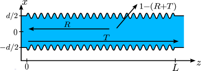
Figure 1: Model of corrugated waveguide. Transmittance $T$, reflectivity $R$, and losses $1-(R+T)$. The (mean) width of the waveguide is $d=450$nm, the length $L=10d=4.5\mu m$. The refractive index of the inner (outer) material is $n=2$ ($n=1$). The wavelength of the boundary oscillation is $\Lambda=200$nm, and its amplitude is $A=37.5$nm ($\sigma=37.5\textrm{nm}/\sqrt{2}$).

Coupled mode theory is a powerful and common method Yariv and Yeh (2003). The starting point is the wave equation for a dielectric waveguide with permeability $\mu$ and dielectric function $\epsilon(x,y)$, which is weakly perturbed by $\Delta\varepsilon(x,y,z)$, written as

$$\left[\nabla^{2}+\omega^{2}\mu(\epsilon+\Delta\epsilon)\right]\vec{E}(x,y,z)=0.$$ (2)

The field $\vec{E}$ of frequency $\omega=kc$ can be constructed from the Eigenfunctions $E_{l}$ of the unperturbed waveguide. The contribution $A_{l}$ of each Eigenmode $E_{l}$, changes along the waveguide, due to the dielectric perturbation, such that

$$\vec{E}=\sum_{l}A_{l}(z)\vec{E}_{l}(x,y)e^{i(\omega t-\beta_{m}z)}$$ (3)

where $\beta_{m}$ is the propagation constant of the $m$’th mode. This is, the component of the wave vector in propagation $z$-direction. Inserting Eq. (3) into Eq. (2) and taking the scalar product with $E^{*}_{k}$ yields (see Yariv and Yeh (2003) for details)

$$\frac{d}{dz}A_{k}=-i\frac{\beta_{k}}{|\beta_{k}|}\sum_{l}C^{(b)}_{kl}A_{l}e^{i(\beta_{k}-\beta_{l})z}$$ (4)

where the changes in $A_{l}$ are assumed to be sufficiently “slow” to neglect $\frac{d^{2}A_{l}}{dz^{2}}$ (see Yariv and Yeh (2003)). The coupling coefficient

$$C^{(b)}_{kl}=\frac{\omega}{u}\int dxdy\vec{E}_{k}\Delta\epsilon\vec{E}_{l}$$ (5)

describing the overlap between two modes $k$ and $l$. The coefficient $u$ accounts for different possible choices of the normalization of $\vec{E}_{k}$. In the following, we will restrict ourselves to two modes. In this case Eq. (4) is a set of two coupled equations $(k=1,l=2$ and $k\leftrightarrow l$)

$$\frac{d}{dz}A_{1} =-i\frac{\beta_{1}}{|\beta_{1}|}\sum_{2}C^{(b)}_{12}A_{2}e^{i(\beta_{1}-\beta_{2})z}$$ (6)

$$\frac{d}{dz}A_{2} =-i\frac{\beta_{2}}{|\beta_{2}|}\sum_{1}C^{(b)}_{21}A_{1}e^{i(\beta_{2}-\beta_{1})z}$$ (7)

A relevant figure is the reflectivity of a system. Solving these coupled mode equations yields two solutions $A_{1},A_{2}$. The ratio of these two solutions at the beginning of the sample ($z=0$), is the ratio of incoming to backscattered mode, i.e., the reflectivity

$$R =\left|\frac{A_{2}(0)}{A_{1}(0)}\right|^{2}$$ (8)

When solving Eq. (6) and Eq. (7) and plugging the solution into Eq. (8), the maximum reflectivity is obtained as

$$R_{max}=\tanh^{2}\left(\hat{C}^{(b)}_{kl}L\right)$$ (9)

where $\hat{C}_{kl}$ is the Fourier coefficient in the Fourier series of $C_{kl}$ (as in Eq. (10)).

A common simplification is to assume that the dielectric perturbation is periodic in $z$ Flanders et al. (1974); Kogelnik (1975)

$$\Delta\epsilon(x,y,z)=\sum_{m}\epsilon_{m}(x,y)e^{-im\frac{2\pi}{\Lambda}z}$$

Then the $z$-dependence of $\Delta\epsilon(x,y,z)$ can be separated from the overlap integral in Eq. (5), which is only over $x$ and $y$.

$$C^{(b)}_{kl}=\frac{\omega}{u}\sum_{m}e^{-im\frac{2\pi}{\Lambda}z}\int dxdy\vec{E}_{k}\epsilon_{m}(x,y)\vec{E}_{l}$$ (10)

This means, in particular, that the integral becomes independent of $z$. In fact we reduced the description of coupling effects to a stratified waveguide. This is, a waveguide which is composed of rectangular slices, each with some $\Delta\epsilon$. This is not surprising, because we constructed the E-Field as contributions of Eigenfunctions, weighted by $A_{l}$ in Eq. (3). We assumed that the $(x,y,z)$-dependencies of the E-Field can be separated into $A_{l}(z)$ and the Eigenmodes $E_{l}(x,y)$. However, if we then try to tackle an arbitrary corrugated waveguide, we have to keep in mind that the only results we can expect are results for stratified waveguides. Common text book approaches ignore this fact Yariv and Yeh (2003); Kogelnik (1975); Ebeling (2011).

III coordinate transformation

Corrugated waveguides feature rich physical effects which are not present in stratified waveguides. Therefore, as a next step we will show how to overcome the shortcomings of common coupled mode theory, without rejecting the entire approach, which, indeed, captivates by its clarity and simplicity.

As the above problems are of geometrical nature, i.e., restriction to stratified waveguides, it is reasonable to look for a geometrical solution. Here we use a straightforward coordinate transformation to transform the corrugated boundaries to flat boundaries.

This transformation has been used previously to derive the square gradient scattering mechanism in systems that feature boundaries with randomized roughness Izrailev et al. (2006). Even though this was the very first derivation of the square gradient mechanism, the general validity of this mechanism was so far doubtful for several reasons. At first it is derived for ensembles of systems that feature peculiar statistical properties. Therefore it is not a priori clear if the mechanism is only a statistical effect. Previous experiments Dietz et al. (2012) investigated systems that resembled these special statistical properties. Furthermore, both theory and experiment have so far being restricted to hollow waveguides with perfectly electrically conducting boundaries.

In the following, we will put the square gradient scattering mechanism on solid theoretical grounds for individual systems, with arbitrary boundaries. This will be done for dielectric waveguides, but we will show that our general results are valid for perfect electric conductors as well.

We assume a waveguide as shown in Fig. 1. The waveguide has a width $d$ whose boundaries are given by a normalized boundary function $q(z)$, such that the boundaries are at $x=\pm d/2\pm\sigma q$, where $\sigma^{2}$ is the variance of the boundary. For a sinusoidal boundary $\sigma$ is connected to the amplitude $A$ of the oscillation of the boundary by $\sigma=A/\sqrt{2}$. We chose the coordinate transformation as

$$(x,y,z) \rightarrow(\frac{w(\tilde{z})}{d}\tilde{x},\tilde{y},\tilde{z}) \textrm{with }w(\tilde{z})=d+2\sigma q(\tilde{z})$$ (11)

It will flatten the boundaries of the dielectric waveguide at $\tilde{x}=\pm d/2$ and thus set $\Delta\epsilon=0$ in Eq. (2), yielding

$$\left[\widetilde{\nabla}^{2}+\omega^{2}\mu\tilde{\epsilon}_{0}(\tilde{x},\tilde{y})\right]\vec{E}(\tilde{x},\tilde{y},\tilde{z})=0$$ (12)

The transformed Laplacian $\widetilde{\nabla}^{2}$ consists of several new terms

$$\widetilde{\nabla}^{2} =\widetilde{\nabla}_{\textrm{red}}^{2}+\tilde{\nabla}_{b}^{2}+\tilde{\nabla}_{x}^{2}+\tilde{\nabla}_{sg}^{2}$$ (13)

which are calculated in Appendix A. Here, the reduced Laplacian is defined as

$$\widetilde{\nabla}_{\textrm{red}}^{2} :=\frac{\partial^{2}}{\partial\tilde{x}^{2}}+\frac{\partial^{2}}{\partial\tilde{y}^{2}}+\frac{\partial^{2}}{\partial\tilde{z}^{2}}$$ (14)

The other terms will now be interpreted as the new dielectric perturbation $\Delta\tilde{\epsilon}$

$$\tilde{\nabla}_{b}^{2}+\tilde{\nabla}_{x}^{2}+\tilde{\nabla}_{sg}^{2}=:\omega^{2}\mu\Delta\tilde{\epsilon}$$ (15)

yielding the transformed wave equation

$$\left[\widetilde{\nabla}_{\textrm{red}}^{2}\right. +\left.\omega^{2}\mu\left(\tilde{\epsilon}_{0}(\tilde{x},\tilde{y})+\Delta\tilde{\epsilon}\right)\right]\vec{E}(\tilde{x},\tilde{y},\tilde{z})=0$$ (16)

In the next three sections the three terms in Eq. (13) will be studied in detail. It will be shown that $\tilde{\nabla}^{2}_{b}$ yields the well-known Bragg reflection (therefore index $b$). It is analog to previous stratified approximations. Frequency analysis shows that $\tilde{\nabla}^{2}_{x}$ can be safely neglected. Finally the last term, $\tilde{\nabla}_{sg}^{2}$ will turn out to represent the novel mechanism of square gradient Bragg reflection (index $sg$).

IV Stratified approximation yields Bragg scattering

The first term

$$\tilde{\nabla}_{b}^{2} =\left(\frac{d^{2}}{w^{2}}-1\right)\frac{\partial^{2}}{\partial\tilde{x}^{2}}$$ (17)

contains no derivative of $q(z)$. In this term the curvature of the boundary has no influence. The physical effects expected from $\tilde{\nabla}_{b}^{2}$ are those of the stratified waveguide. To work out the physical influence of $\tilde{\nabla}^{2}_{b}$ we ignore the two other terms in Eq. (15) and set

$$\Delta\tilde{\epsilon}=\frac{1}{\omega^{2}\mu}\left(\frac{d^{2}}{w^{2}}-1\right)\frac{\partial^{2}}{\partial\tilde{x}^{2}}$$ (18)

The coupling coefficient from Eq. (5) becomes

$$C^{(b)}_{kl}=\frac{\omega}{u}\int\int d\tilde{x}d\tilde{y}\frac{w}{d}\vec{\tilde{E_{k}}}\Delta\tilde{\epsilon}\vec{\tilde{E_{l}}}$$ (19)

where the prefactor is the Jacobian $dxdy=d\tilde{x}d\tilde{y}\left|\frac{w}{d}\right|$, which is strictly positive, so that $|\frac{w}{d}|=\frac{w}{d}$. The modes of the electric field $\vec{\tilde{E_{k}}},\vec{\tilde{E_{l}}}$, are the undisturbed modes of the transformed system, i.e., $\Delta\tilde{\epsilon}=0$ in Eq. (16). These modes are calculated in Appendix B.

Plugging Eq. (18) into Eq. (19), yields

$$C^{(b)}_{kl} =\left(\frac{d}{w}-\frac{w}{d}\right)\frac{1}{p\omega\mu}\int\int d\tilde{x}d\tilde{y}\vec{\tilde{E_{k}}}\frac{\partial^{2}}{\partial\tilde{x}^{2}}\vec{\tilde{E_{l}}}$$ (20)

Approximating

$$\left(\frac{d}{w}-\frac{w}{d}\right)=-4\frac{\sigma}{d}q(z)\left(\frac{d+\sigma q}{d+2\sigma q}\right)\approx-4\frac{\sigma}{d}q(z)$$

we have

$$C^{(b)}_{kl} =q(z)I_{kl}^{(b)}$$ (21)

where

$$I^{(b)}_{kl}=-\frac{\sigma}{d}\frac{4}{p\omega\mu}\int\int d\tilde{x}d\tilde{y}\vec{\tilde{E_{k}}}\frac{\partial^{2}}{\partial\tilde{x}^{2}}\vec{\tilde{E_{l}}}$$ (22)

The coupling coefficient can now be readily calculated for given material parameters. Before doing so, we show, that the first term in Eq. (15) indeed corresponds to Bragg scattering. To this end, we analyze the periodicity of $C^{(b)}_{kl}$, which is clearly the same as the periodicity of the corrugated boundary $q(z)$. Assuming that $q(z)$ is a periodic function it can be expanded as

$$q(z)=\sum_{m}q^{(b)}_{m}\,e^{-im\frac{2\pi}{\Lambda}\tilde{z}}$$ (23)

We can thus write

$$C^{(b)}_{kl} =\sum_{m}q^{(b)}_{m}\,I^{(b)}_{kl}e^{-im\frac{2\pi}{\Lambda}\tilde{z}}$$ (24)

and set $\hat{C}^{(b)}_{kl}=q^{(b)}_{m}I^{(b)}_{kl}$.

As in Yariv and Yeh (2003), we now analyze small changes in the amplitude $A(z)$ in Eq. (4) by integrating over a length $s$, which is long compared to $\Lambda$

$$dA_{k}\sim\sum_{l}\sum_{m}\int_{s}\hat{C}^{(b)}_{kl}A_{l}e^{i(\beta_{k}-\beta_{l}-m\frac{2\pi}{\Lambda})z}\,dz$$ (26)

This integral will vanish unless the Bragg condition

$$\beta_{k}-\beta_{l}=m\frac{2\pi}{\Lambda}$$ (27)

is satisfied. In case of backscattering into the same mode ($\beta_{k}=-\beta_{l}$)the Bragg condition takes the form

$$\beta_{k}=m\frac{\pi}{\Lambda}$$ (28)

which is Eq. (1) for lattice spacing $d=\Lambda$.

We have thus shown, that the first term of the transformation yields the well known Bragg scattering. What about the different order $m$? For a sinusoidal boundary $q(z)\sim\sin(\frac{2\pi}{\Lambda}z)$, there are only two possible values $m=\pm 1$ in Eq. (23), which yield the same wavelength. Consequently, there is only one single reflection resonance predicted in the stratified approximation.

After we have successfully recovered the results for the stratified approximation we will now turn to the next term.

V Beyond Bragg scattering

The second term $\tilde{\nabla}^{2}_{x}$, comprises derivatives of $q(z)$.

$$\tilde{\nabla}_{x}^{2} =-\frac{\sigma}{w}\left(\frac{\partial q}{\partial\tilde{z}}\tilde{x}\left(\frac{\partial}{\partial\tilde{x}}\frac{\partial}{\partial\tilde{z}}+\frac{\partial}{\partial\tilde{z}}\frac{\partial}{\partial\tilde{x}}\right)\right.$$

$$+\left.\frac{\partial^{2}q}{\partial\tilde{z}^{2}}\tilde{x}\frac{\partial}{\partial\tilde{x}}\right)$$

Here the curvature of the boundary influences the scattering. This is the first indication that we no longer deal with a stratified system. However terms in $\nabla^{2}_{x}$ will have the same periodicity as $q(z)$ itself and come into play at frequencies given by the Bragg condition. This means that they act at the exact same frequencies as the terms used in the stratified approximation. We will neglect this term here, because in this study we are interested in reflection resonance that take place at frequencies other than the Bragg resonances.

In contrast, the third term on the left hand side of Eq. (15) contains terms with the square of the derivative of $q(z)$. In general the square of a function can have a different periodicity than $q(z)$. Therefore we expect this term to play a role at frequencies different from that given by the Bragg condition:

$$\tilde{\nabla}_{sg}^{2} =\frac{\sigma^{2}}{w^{2}}\left(\frac{\partial q}{\partial\tilde{z}}\right)^{2}\left(3\tilde{x}\frac{\partial}{\partial\tilde{x}}+\tilde{x}^{2}\frac{\partial^{2}}{\partial\tilde{x}^{2}}\right)$$ (29)

which yields

$$C^{(sg)}_{kl} =\left(\frac{\partial q}{\partial\tilde{z}}\right)^{2}I^{(sg)}_{kl}$$ (30)

where, the overlap integral is obtained after approximating $$w=d$$ (see Eq. (11)), as

$$I^{(sg)}_{kl} \approx\frac{\sigma^{2}}{d^{2}}\frac{1}{u\omega\mu}\int d\tilde{x}d\tilde{y}\vec{\tilde{E_{k}}}\left(3\tilde{x}\frac{\partial}{\partial\tilde{x}}+\tilde{x}^{2}\frac{\partial^{2}}{\partial\tilde{x}^{2}}\right)\vec{\tilde{E_{l}}}$$ (31)

Following the arguments yielding the Bragg condition Eq. (28), we can expand

$$\left(\frac{\partial q}{\partial\tilde{z}}\right)^{2}=\sum_{m^{\prime}}p^{(sg)}_{m^{\prime}}\,e^{-im^{\prime}\frac{2\pi}{\Lambda}\tilde{z}}$$

and derive a square gradient Bragg condition

$$\beta_{k}-\beta_{l}=m^{\prime}\frac{2\pi}{\Lambda}$$ (32)

For backscattering into the same mode ($\beta_{k}=-\beta_{l}$) it reads

$$\beta_{k}=m^{\prime}\frac{\pi}{\Lambda}$$ (33)

This looks just like the ordinary Bragg condition, but note, that here we have expanded the square gradient. To see the difference we consider a specific boundary $q(z)\sim\sin(\frac{2\pi}{\Lambda}z)$. The Fourier series of the square gradient of $q(z)$ reads

$$\left(\frac{\partial\sin(\frac{2\pi}{\Lambda}z)}{\partial z}\right)^{2}=\left(\frac{2\pi}{\Lambda}\right)^{2}\left(\frac{1}{2}+\frac{1}{4}e^{-i\frac{4\pi}{\Lambda}z}+\frac{1}{4}e^{i\frac{4\pi}{\Lambda}z}\right)$$ (34)

In contrast to the Bragg condition ($m=\pm 1$), here we have two contributions $m^{\prime}=0$ and $m^{\prime}=2$. This means, that the square gradient Bragg scattering impacts the transmission at two disjunct frequencies.

Plugging $m=0$ into the square gradient Bragg condition Eq. (33), shows that backscattering into the same mode ($\beta_{k}=-\beta_{l}$) occurs for $\beta_{k}\rightarrow 0$. In symmetric dielectric waveguides (as the exemplary waveguide, we discuss) this effect is not present because modes have a non-zero cut-off frequency. This means, that for small wave vectors there is no guided mode that could be affected by the $m=0$ scattering. For asymmetric dielectric waveguides it should in principle be possible to observe strong backscattering due to square gradient Bragg reflection for $\beta\rightarrow 0$. This effect has been demonstrated experimentally within the statistical approach for perfectly conducting metallic waveguides the do not have cut-off frequencies Dietz et al. (2012). We will show that our theoretical framework covers these results as well. However, contrast to the statistical approach Izrailev et al. (2006), which works only for boundaries that feature peculiar statistic features our approach covers arbitrary shaped boundaries. In particular, we are not longer restricted to (pseudo) random boundaries.

The second contribution is $m=2$. It operates at half the wavelength of ordinary Bragg scattering. This is in fact a general feature. Every boundary that obeys

$$q(z+\Lambda/2)=-q(z)$$

will exhibit square gradient Bragg resonances at half the wavelenght of the Bragg resonance. This is, because the square of such a $q$ will have a periodicity $\Lambda/2$.

In contrast to Bragg scattering the frequency domain where square gradient Bragg scattering occurs didn’t attract much attention, presumably because there was no further Bragg order expected or the square gradient Bragg resonance was confused with higher order Bragg resonances. Therefore, this reflection resonance has – to our knowledge – not been observed or identified experimentally.

VI Coupled mode equations for arbitrary boundaries

So far we have qualitatively investigated infinite periodic systems, that could be expanded in a Fourier series. In this sections it is shown how arbitrary (finite) boundary profiles can be treated quantitatively. We will see that the Bragg condition will be replaced by its continuous counter-part, the Fourier transform of the boundary. So, instead of expanding the boundary as a Fourier series, it will now be represented as a Fourier transformation. This means dropping the assumption of a periodic function.

$$q(\tilde{z}) =\sum_{m}q^{(b)}_{m}e^{-im\frac{2\pi}{\Lambda}z}\rightarrow\int d\beta q_{b}(\beta)e^{-i\beta z}$$ (35)

To obtain the Bragg condition in the continuous case, the $dA_{k}$ is, as in Eq. (26), integrated over a small domain $s$:

$$dA_{k} =-i\frac{\beta_{k}}{|\beta_{k}|}\sum_{l}\int d\beta q_{b}(\beta)\underbrace{\int_{s}dz\,I^{(b)}_{kl}A_{l}e^{i(\beta_{k}-\beta_{l}-\beta)z}}_{\rightarrow 0,\,\forall\,\beta_{k}-\beta_{l}\neq\beta}$$ (36)

The exponential function in the second integral oscillates and will thus be zero, as long as $$\beta_{k}-\beta_{l}\neq\beta \delta$$. Therefore, the result can be approximated by a normalized -Function

$$dA_{k} \approx-i\frac{\beta_{k}}{|\beta_{k}|}\sum_{l}\int d\beta q_{b}(\beta)N\delta(\beta_{k}-\beta_{l}-\beta)\int_{s}dz\,I^{(b)}_{kl}A_{l}$$ (37)

$$=-i\frac{\beta_{k}}{|\beta_{k}|}\sum_{l}Nq_{b}(\beta_{k}-\beta_{l})\int_{s}dz\,I^{(b)}_{kl}A_{l}$$ (38)

and in case of backscattering, where $$\beta_{k}=-\beta_{l}$$

$$=-i\frac{\beta_{k}}{|\beta_{k}|}\sum_{l}Nq_{b}(2\beta_{k})\int_{s}dz\,I^{(b)}_{kl}A_{l}$$ (39)

The normalization $N$ is discussed below. The coupling is thus proportional to $q_{b}(2\beta_{k})$. This line of reasoning holds for both $q_{b}(\beta)$ (Bragg scattering) and $q_{sg}(\beta)$ (square gradient Bragg scattering). Instead of discrete conditions Eq. (28) and Eq. (33) we now have a continuous range where scattering can occur. This continuous range is given by the Fourier transformations $q_{b/sg}$ of the boundary and the square of the curvature of the boundary. Taking the derivative of Eq. (38) yields a generalized coupled mode equation for arbitrary boundaries (compareEq. (4))

$$\frac{dA_{k}}{dz} =-i\frac{\beta_{k}}{|\beta_{k}|}N\sum_{l}q_{b}(\beta_{k}-\beta_{l})I^{(b)}_{kl}A_{l}$$ (40)

As before, investigating two modes, yields a set of two coupled equations ($k=1,l=2$ and $k=2,l=1$). Solving this set for contra-directional coupling ($\beta_{1}=-\beta_{2}$), yields two solution, one for the incoming mode $A_{1}$ and one for the backscattered mode $A_{2}$. As before, the reflectivity is given by the ratio of the incoming and the backscattered mode. Plugging in the solutions, they evaluate to

$$R^{(b)}_{kl} =\left|\frac{A_{2}(0)}{A_{1}(0)}\right|^{2}=|\tanh\left(Nq_{b}(\beta_{1}-\beta_{2})I^{(b)}_{kl}L\right)|^{2}$$ (41)

for Bragg scattering. Starting from $$p^{(sg)} I^{(sg)}_{kl}$$ and instead we arrive at the result for square gradient Bragg scattering

$$R^{(sg)}_{kl} =\left|\frac{A_{2}(0)}{A_{1}(0)}\right|^{2}=|\tanh\left(Nq_{sg}(\beta_{1}-\beta_{2})I^{(sg)}_{kl}L\right)|^{2}$$ (42)

This is the main result of this paper, and shall be discussed in detail. At first, it is in perfect agreement with the maximum reflectivity in the periodic case, Eq. (9). By comparing Eq. (9) and Eq. (41) we can fix the normalization $N$. The result of the two approaches has to be the same when evaluating the coupling of two modes in an infinite sample over a range $L$ or in a finite system of length $L$. Thus setting $Nq_{b}(\beta_{b})=p_{m=1}$, yields $N=\frac{2\pi}{L}$.

At this point we are able to show, that our results include the previous results from the statistical approach Izrailev et al. (2006). When assuming a perfectly electric conducting hollow waveguide $q_{b}I^{(q)}_{kl}$ and $q_{sg}I^{(sg)}_{kl}$ evaluate to (see Appendix D)

$$\left(q_{b}I^{(b)}_{kl}\right)^{2} =\frac{1}{L_{n}^{(b),(AS)}}$$ (43)

$$\left(q_{sg}I^{(sg)}_{kl}\right)^{2} =\frac{1}{L_{n}^{(b),(SGS)}}$$ (44)

for even modes. $L_{n}^{(b),(AS/SGS)}$ is the backscattering length derived in Izrailev et al. (2006). In contrast to Izrailev et al. (2006), we find different results for odd and even modes. However, it seems that the authors of Izrailev et al. (2006) were unaware that they studied a symmetry reduced version of the system. Therefore their results are only valid for modes with $E(z=0)=0$, i.e., even modes.

This means that we derived the very same expression under drastically relaxed assumptions. First, our result is valid for any boundary and the reflectivity is directly calculated from the boundary in a straightforward way. A cumbersome generation procedure to generate random boundaries that comply with the statistical requirements of the statistical approach (see Dietz et al. (2012); Doppler et al. (2014)) are not necessary. Second, the derivation does not depend on the type of boundary. Previous studies were bound to perfectly electric conducting boundary conditions. Therefore they could not be applied to dielectric waveguides, where the mode crosses the boundary and penetrates the region outside the waveguide.

VII Reflectivity of a dielectric Waveguide

Now the reflectivity for a dielectric waveguide can be calculated in a straight forward manner. By inserting the modes of the E-Field (see Appendix B) into Eq. (22) and Eq.  (31), $I^{(b)}_{kl}$ and $I^{(sg)}_{kl}$ are obtained. The Fourier transformation of the boundary $q_{b}$ and of the curvature of the boundary are calculated in the Appendix C. Inserting these quantities into Eq. (41) and Eq. (42) yields the reflectivity. As an example, we investigate the first mode in the waveguide shown in Fig. 1. In Fig. 2 a) and b) the calculated reflectivity $R$ and the transmission $T$, respectively, are displayed as a function of (vacuum) wave vector $k$. Two sharp peaks caused by Bragg scattering into the same mode $R^{(b)}_{11}$ and into the next odd mode $R^{(b)}_{13}$ can be clearly identified. The new square gradient Bragg reflection resonances $R^{(sg)}_{11},$ and $R^{(sg)}_{13}$ occur as expected at twice the value of $\beta$. From this calculations it is apparent that square gradient Bragg scattering is as strong as Bragg scattering. Note that these square gradient peaks must not be confused with conventional higher order Bragg peaks. In this waveguide with sinusoidal boundaries, there are no conventional higher order Bragg terms, since the boundary has only a single frequency component.

VIII Comparison to numerical results

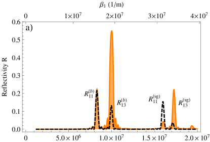
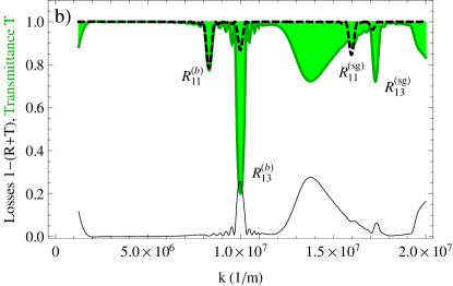
Figure 2: a) Reflectivity of first mode through the dielectric waveguide shown in Fig. 1. Analytical prediction (dashed black,      ) calculate from Eq. (41) and Eq. (42) in comparison to numerical data (orange,  ). b) Analytical transmittance calculated from reflectivity in a) as $T=1-R$ (dashed black,      ) compared to numerical transmission (green,  ). The difference in both are the radiation losses $1-(R+T)$ (black,  ).

To test our analytical predictions numerically we use a commercial finite element solver (JCMwave). The Maxwell equations are solved on a non-uniform 2d mesh. Convergence was tested and confirmed by increasing the finite element degree up to 7 Hoffmann et al. (2009). Fig. 2 compares the analytical to the numerical results for the structure displayed in Fig. 1. We see in Fig. 2  a) that for Bragg scattering into the same mode , $R^{(b)}_{11}$, the calculated reflectivity is in perfect agreement with the numerical results. The situation is different for the square gradient Bragg scattering into the same mode $R^{(sg)}_{11}$. The peak is clearly visible, but overestimated by the theory. For inter-mode scattering $R^{(b)}_{13}$ and $R^{(sg)}_{13}$, the situation is reversed. The reflection resonance is much stronger than predicted by the theory, for both scattering mechanisms. This is surprising, because the overlap integral in $C^{(i)}_{kl}$, Eq. (19), is obviously smaller for modes where $k\neq l$ compared to $k=l$, where the overlap is maximal. The origin of the strongly enhanced inter-mode scattering has to be investigated more thoroughly, in a framework beyond two-wave coupled mode theory.

To investigate the influence of square gradient Bragg scattering on the transmission, we numerically calculated the transmission: the result (green,  ) is shown in Fig. 2 b). It is compared to the analytical transmission (dashed black,      ), calculated from the reflectivity $T=1-R$. As expected, the reflection resonances appear as gaps in the transmission. Still, the transmission shows strong deviation, from $R+T=1$, due to radiation losses.

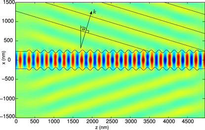
Figure 3: E-Field ($\textrm{Re}(E_{y})$) at maximum of radiation losses at $k=1.4\cdot 10^{7}/m$ (compare dip in Fig. 2 b). Plane waves radiate out of the waveguide (dashed lines). The expected $k$-vector from Eq. (45) is indicated ($\Theta=$$$).

To investigate the influence of radiation losses, we plotted the losses as $1-(R+T)$ (black,  ) in Fig. 2 b). Most apparent is the broad gap around $k=1.4\cdot 10^{7}/$m. It stems from light that is coupled out of the waveguide by coupling to radiation modes $\beta_{out}=nk\sin\Theta$

$$kn\sin\Theta+\frac{2\pi}{\Lambda} =\beta_{k}$$ (45)

where $n$ is the refractive index of the outer material and $\beta_{k}$ is, as before, the propagation constant of the guided mode. Eq. (45) yields (with parameters from Fig. 1) an outcoupling angle of $\Theta=$$$ (measured counter clockwise from the $x$-axis), which is in perfect agreement with the numerically calculated maximum (Fig. 3).

The second important feature are the strong scattering losses at the $R^{(b)}_{13}$ reflection resonance. Around 25% of the transmission is lost due to radiation out of the waveguide. The effect is smaller ($\sim 15\%$) for curved Bragg scattering, $R^{(sg)}_{13}$, but still visible.

A general observation when comparing the analytical to the numerical data is that the reflection into the same mode is overestimated, while backscattering into higher modes is underestimated by the generalized coupled mode theory. The transmittance is further reduced by radiation losses at the (square gradient) Bragg resonances.

IX Summary

We showed the appearance of unexpected Bragg resonances in dielectric waveguides with corrugated boundaries. We generalized a statistical approach to cover individual systems with arbitrary boundaries.

The analytically calculated reflectivity is in good agreement with the numerical results. While the position of the expected resonance is predicted with high accuracy, the strength of the square gradient Bragg scattering is strongly underestimated. We find that Bragg and square gradient Bragg scattering are of comparable strength.

The transmission through the waveguide is even stronger affected by the square gradient Bragg reflections due to radiation losses.

Since Bragg scattering is one of the key properties in corrugated waveguides. A general theory which is able to describe all Bragg resonances is a promising new tool for designing optical systems based on waveguide structures. For example, in directional couplers, coupling and reflecting gratings are combined Kewes et al. (2015). Both gratings have to have different periodicity. Using the square gradient Bragg scattering mechanism it should be possible to use the same grating for coupling and reflection purposes. This would considerably simplify grating structures.

X Acknowledgments

O.D. expresses his gratitude to Stefan Rotter (TU Vienna) for his encouraging critique on the early version of this paper. He likes to thank Dan-Nha Huynh and Matthias Moeferdt for fruitful discussion. Support by SFB 787 is acknowledged by O.D.

Appendix A Explicit calculation of the coordinate transformation

The differential operator in the new coordinates

$$(x,y,z) \rightarrow(\frac{w(\tilde{z})}{d}\tilde{x},\tilde{y},\tilde{z}) \textrm{with }w(\tilde{z})=d+2\sigma q(\tilde{z})$$

is derived in the following. For some function $q(\tilde{x},\tilde{y},\tilde{z})$ we obtain

$$\frac{\partial}{\partial x}q =\left(\frac{\partial\tilde{x}}{\partial x}\frac{\partial}{\partial\tilde{x}}+\frac{\partial\tilde{y}}{\partial x}\frac{\partial}{\partial\tilde{y}}+\frac{\partial\tilde{z}}{\partial x}\frac{\partial}{\partial\tilde{z}}\right)q$$

$$=\left(\frac{\partial\tilde{x}}{\partial x}\frac{\partial}{\partial\tilde{x}}\right)q=\frac{d}{w}\frac{\partial}{\partial\tilde{x}}q$$

$$\frac{\partial}{\partial y}q =\left(\frac{\partial\tilde{x}}{\partial y}\frac{\partial}{\partial\tilde{x}}+\frac{\partial\tilde{y}}{\partial y}\frac{\partial}{\partial\tilde{y}}+\frac{\partial\tilde{z}}{\partial y}\frac{\partial}{\partial\tilde{z}}\right)q=\frac{\partial}{\partial\tilde{y}}q$$

$$\frac{\partial}{\partial z}q =\left(\frac{\partial\tilde{x}}{\partial z}\frac{\partial}{\partial\tilde{x}}+\frac{\partial\tilde{y}}{\partial z}\frac{\partial}{\partial\tilde{y}}+\frac{\partial\tilde{z}}{\partial z}\frac{\partial}{\partial\tilde{z}}\right)q$$

$$=\left(\frac{\partial\tilde{x}}{\partial z}\frac{\partial}{\partial\tilde{x}}+\frac{\partial}{\partial\tilde{z}}\right)q$$

$$=\left(\frac{dx\sigma}{-w(\tilde{z})^{2}}\frac{\partial q}{\partial\tilde{z}}\frac{\partial}{\partial\tilde{x}}+\frac{\partial}{\partial\tilde{z}}\right)q$$

$$=\left(\underbrace{\tilde{x}\frac{\sigma}{-w(\tilde{z})}\frac{\partial q}{\partial\tilde{z}}\frac{\partial}{\partial\tilde{x}}}_{A}+\underbrace{\frac{\partial}{\partial\tilde{z}}}_{B}\right)q$$

where $A$, and $B$, label the terms for better tracking. Applying the derivation twice yields

$$\frac{\partial^{2}}{\partial x^{2}}q =\frac{d^{2}}{w^{2}}\frac{\partial^{2}}{\partial\tilde{x}^{2}}q$$

$$\frac{\partial^{2}}{\partial y^{2}}q =\frac{\partial^{2}}{\partial\tilde{y}^{2}}q$$

$$\frac{\partial^{2}}{\partial z^{2}}q =\left(\underbrace{\tilde{x}\frac{\sigma^{2}}{w^{2}}\left(\frac{\partial q}{\partial\tilde{z}}\right)^{2}\frac{\partial}{\partial\tilde{x}}+\tilde{x}^{2}\frac{\sigma^{2}}{w^{2}}\left(\frac{\partial q}{\partial\tilde{z}}\right)^{2}\frac{\partial^{2}}{\partial\tilde{x}^{2}}}_{A^{2}}\right.$$

$$+\underbrace{\tilde{x}\frac{\sigma}{-w}\frac{\partial q}{\partial\tilde{z}}\frac{\partial}{\partial\tilde{x}}\frac{\partial}{\partial\tilde{z}}}_{AB}+\underbrace{\frac{\partial}{\partial\tilde{z}}\tilde{x}\frac{\sigma}{-w(\tilde{z})}\frac{\partial q}{\partial\tilde{z}}\frac{\partial}{\partial\tilde{x}}}_{BA}$$

$$+\left.\underbrace{\frac{\partial^{2}}{\partial\tilde{z}^{2}}}_{B^{2}}\right)q$$

where the last term becomes

$$\frac{\partial}{\partial\tilde{z}}\tilde{x}\frac{\sigma}{-w(\tilde{z})}\frac{\partial q}{\partial\tilde{z}}\frac{\partial}{\partial\tilde{x}}$$

$$=\frac{\tilde{x}\sigma^{2}}{w^{2}}\left(\frac{\partial q}{\partial\tilde{z}}\right)^{2}\frac{\partial}{\partial\tilde{x}}+\frac{\tilde{x}\sigma^{2}}{w^{2}}\left(\frac{\partial q}{\partial\tilde{z}}\right)^{2}\frac{\partial}{\partial\tilde{x}}$$

$$+\frac{\tilde{x}\sigma}{-w}\left(\frac{\partial^{2}q}{\partial\tilde{z}^{2}}\right)\frac{\partial}{\partial\tilde{x}}+\frac{\tilde{x}\sigma}{-w}\frac{\partial q}{\partial\tilde{z}}\frac{\partial}{\partial\tilde{z}}\frac{\partial}{\partial\tilde{x}}$$

There appear different types of derivatives of $q$. Grouping these terms using the reduced Laplacian defined in Eq. (14)

$$\widetilde{\nabla}^{2} =\widetilde{\nabla}_{\textrm{red}}^{2}+\tilde{\nabla}_{b}^{2}+\tilde{\nabla}_{x}^{2}+\tilde{\nabla}_{sg}^{2}$$

we have

$$\tilde{\nabla}_{b}^{2} =\left(\frac{d^{2}}{w^{2}}-1\right)\frac{\partial^{2}}{\partial\tilde{x}^{2}}$$

$$\tilde{\nabla}_{x}^{2} =-\frac{\sigma}{w}\frac{\partial q}{\partial\tilde{z}}\tilde{x}\left(\frac{\partial}{\partial\tilde{x}}\frac{\partial}{\partial\tilde{z}}+\frac{\partial}{\partial\tilde{z}}\frac{\partial}{\partial\tilde{x}}\right)-\frac{\sigma}{w}\left(\frac{\partial^{2}q}{\partial\tilde{z}^{2}}\right)\tilde{x}\frac{\partial}{\partial\tilde{x}}$$

$$\tilde{\nabla}_{sg}^{2} =\frac{\sigma^{2}}{w^{2}}\left(\frac{\partial q}{\partial\tilde{z}}\right)^{2}3\tilde{x}\frac{\partial}{\partial\tilde{x}}+\frac{\sigma^{2}}{w^{2}}\left(\frac{\partial q}{\partial\tilde{z}}\right)^{2}\tilde{x}^{2}\frac{\partial^{2}}{\partial\tilde{x}^{2}}$$

Note that only the $x$ coordinate was transformed, hence $\tilde{z}=z$ and $\tilde{y}=y$.

Appendix B Modes of the electric field in dielectric waveguides

Fig. 3 shows the first mode of the electric field in the waveguide. The mode numbers above are chosen to be $k$ and $l$, to identify two specific, but not necessarily different modes. In the following the general index $m$ is used. In the substrate ($\tilde{x}\leq-d/2$) and cover ($d/2\leq\tilde{x}$) regions, the $m$-th mode is given by the E-field perpendicular to the $x$-$z$-plane as (see Kogelnik (1975))

$$\tilde{E}_{m}(\tilde{x},k) =\begin{cases}E_{s}(k)\exp\left(\gamma_{s}\left(\tilde{x}+\frac{d}{2}\right)\right)&\textrm{in substrate}\\ E_{c}(k)\exp\left(-\gamma_{c}\left(\tilde{x}-\frac{d}{2}\right)\right)&\textrm{in cover}\\ \end{cases}$$

and in the film region ($$-d/2<\tilde{x}<d/2$$) odd and even modes are given by

$$\tilde{E}_{m}(\tilde{x},k) =E_{f}(k)\begin{cases}\cos\left(\kappa_{f}\tilde{x}\right)&\textrm{for odd modes}\\ \sin\left(\kappa_{f}\tilde{x}\right)&\textrm{for even modes}\end{cases}$$

with

$$\kappa_{c}^{2} =n_{c}^{2}k^{2}-\beta_{m}^{2}=-\gamma_{c}^{2}$$

$$\kappa_{f}^{2} =n_{f}^{2}k^{2}-\beta_{m}^{2}$$

$$\kappa_{s}^{2} =n_{s}^{2}k^{2}-\beta_{m}^{2}=-\gamma_{s}^{2}$$

Here, the refractive indices refer to the substrate ($n_{s}$), cover ($n_{c}$), and film ($n_{f}$) material. The wave vector $n_{c,f,s}k$ has components in direction of propagation $\beta_{m}$ and in transversal direction denoted by $\kappa_{c,f,s}$. Note, that there is one $\beta_{m}$ for each mode. Consequently $\kappa$ and $\gamma$ depend on the mode number just as $\tilde{E}_{m}$. In the case of a symmetric waveguide the allowed $\beta_{m}$ for each mode $m$ can be found by numerically solving (see Kogelnik (1975))

$$2d\kappa_{f}-4\arctan\sqrt{\frac{1-\left(\frac{n_{s}}{n_{eff}}\right)^{2}}{\left(\frac{n_{f}}{n_{eff}}\right)^{2}-1}}=2\pi m$$

where $n_{eff}=\beta_{m}/|\vec{k}|$. The total normalization is chosen as

$$\frac{2\beta_{m}}{u\omega\mu}\int dxE_{m}^{2}=1\textrm{W/m}$$

and yields the peak field inside the waveguide for odd/even modes

$$E_{f}^{2}=\frac{u\omega\mu}{\beta_{m}}\Bigg{(} d\pm\frac{\sin(d\kappa_{f})}{\kappa_{f}}$$

$$+\frac{n_{f}^{2}-n_{eff}^{2}}{n_{f}^{2}-n_{c}^{2}}\frac{1}{\gamma_{s}}+\frac{n_{f}^{2}-n_{eff}^{2}}{n_{f}^{2}-n_{s}^{2}}\frac{1}{\gamma_{c}}\Bigg{)}^{-1}\textrm{W/m}$$

The amplitudes are connected via

$$E_{f}^{2}(n_{f}^{2}-n_{eff}^{2})=E_{s}^{2}(n_{f}^{2}-n_{s}^{2})=E_{c}^{2}(n_{f}^{2}-n_{c}^{2})$$

Appendix C Fourier Transform $q_{b}$ and $q_{sg}$ of the boundary

Let the (normalized) boundary $q$ of the waveguide (see Fig. 1) be of the simplest possible form:

$$q(z)=\sqrt{2}\sin(\beta_{b}z)\textrm{box}^{L}_{0}(z)$$

where $\beta_{b}=\frac{2\pi}{\Lambda}$ is the periodicity of the boundary and $\textrm{box}^{L}_{0}(z)$ is a box, or rectangular, function of length $L$ constructed via the Heaviside function $\Theta$, as $\textrm{box}^{L}_{0}(z)=\Theta(z)\left(1-\Theta(z-L)\right)$. The wave vector of the boundary roughness $\beta_{b}$ should be chosen in such a way that $\beta_{b}L$ are multiples of $2\pi$ to ensure a continuous function. The Fourier transform is normalized such that

$$q(\beta) =\mathcal{FT}\left(q(z)\right)=\frac{1}{2\pi}\int q(z)\exp\left(i\beta z\right)$$

To calculate $q_{b}$ and $q_{sg}$ the following derivatives with respect to $z$ have to be calculated

$$q^{\prime} =\sqrt{2}\beta_{b}\cos(\beta_{b}z)\textrm{box}^{L}_{0}(z)+\sqrt{2}\sin(\beta_{b}z)\left(\delta(z)-\delta(z-L)\right)$$

$$q^{\prime 2} =2\left(\beta_{b}\cos(\beta_{b}z)\textrm{box}^{L}_{0}(z)\right)^{2}$$

$$\,+2\Big{(}\sin(\beta_{b}z)\left(\delta(z)-\delta(z-L)\right)\Big{)}^{2}$$

$$\,+4\beta_{b}\cos(\beta_{b}z)\textrm{box}^{L}_{0}(z)\sin(\beta_{b}z)\left(\delta(z)-\delta(z-L)\right)$$

Now the Fourier transformation of $q^{\prime 2}$ has to be calculated. However, the boundary profile is chosen in such a way, that it ends at $x=0$, i.e., at the position of the unperturbed boundary. Therefore $\sin(\beta_{b}L)=0$, and thus the second and the third term vanishes since

$$\int \sin^{2}(\beta_{b}z)\left(\delta^{2}(z)-\delta^{2}\left(z-L\right)\right)\exp(-ikz)$$

$$=\sin^{2}(0)\exp(0)-\sin^{2}(\beta_{b}L)\exp(-ikL)$$

$$=0$$

Using $\textrm{box}^{L}_{0}(z)^{2}=\textrm{box}^{L}_{0}(z)$ and rewriting the square of the cosine as sum of two cosines, yields

$$\mathcal{FT}\left(q^{\prime 2}\right) =2\beta_{b}^{2}\mathcal{FT}\left(\cos(\beta_{b}z)^{2}\textrm{box}^{L}_{0}(z)^{2}\right)$$

$$=2\beta_{b}^{2}\mathcal{FT}\left(\left(\cos(0)+\cos(2\beta_{b}z)\right)\textrm{box}^{L}_{0}(z)\right)$$

$$=2\beta_{b}^{2}\mathcal{FT}\left(\textrm{box}^{L}_{0}(z)\right)+\beta_{b}^{2}\mathcal{FT}\left(\cos(2\beta_{b}z)\textrm{box}^{L}_{0}(z)\right)$$

The intermediate result in Fourier representation is

$$\mathcal{FT}\left(q\right) =\sqrt{2}\mathcal{FT}\left(\sin(\beta_{b}z)\textrm{box}^{L}_{0}(z)\right)$$

$$\mathcal{FT}\left(q^{\prime 2}\right) =2\beta_{b}^{2}\left(\mathcal{FT}\left(\textrm{box}^{L}_{0}(z)\right)+\mathcal{FT}\left(\cos(2\beta_{b}z)\textrm{box}^{L}_{0}(z)\right)\right)$$ (46)

With the convolution theorem

$$\mathcal{FT}\left(fg\right)=\mathcal{FT}\left(f\right)*\mathcal{FT}\left(g\right)$$

this result can be further simplified. The ($*$) operator denotes a convolution. Especially interesting for the present case is the convolution with a $\delta$-function, which evaluates as

$$f(z)*\delta(z-b)=f(z-b).$$

Shifting a function, will add an additional phase factor to its Fourier transformation. Therefore instead of evaluating the functions in Eq. (46) directly they will be shifted to be centered around $z=0$. The Fourier transformation of a centered box function is given by

$$\mathcal{FT}\left(\textrm{box}^{L/2}_{-L/2}(z)\right)=\frac{L}{2\pi}\,\textrm{sinc}\left(\frac{\beta L}{2}\right)$$

and the Fourier transformation of the Cosine and Sine is given by

$$\mathcal{FT}\left(\sin{\beta_{b}z}\right) =\frac{i}{2}\delta(\beta-\beta_{b})-\frac{i}{2}\delta(\beta+\beta_{b})$$

$$\mathcal{FT}\left(\cos{2\beta_{b}z}\right) =\frac{1}{2}\delta(\beta-2\beta_{b})+\frac{1}{2}\delta(\beta+2\beta_{b})$$

Applying the convolution theorem and evaluating the $\delta$-functions the resulting expression reads

$$\mathcal{FT}\left(q\right) =\frac{L}{2\pi}\frac{i}{\sqrt{2}}\left(\textrm{sinc}\left(\frac{1}{2}(\beta-\beta_{b})L\right)\right.$$

$$\left.-\textrm{sinc}\left(\frac{1}{2}(\beta+\beta_{b})L\right)\right)$$

$$\mathcal{FT}\left(q^{\prime 2}\right) =\frac{L}{\pi}\beta_{b}^{2}\,\left(\textrm{sinc}\left(\frac{\beta L}{2}\right)+\frac{1}{2}\textrm{sinc}\left(\frac{1}{2}(\beta-2\beta_{b})L\right)\right)$$

$$+\frac{L}{\pi}\beta_{b}^{2}\,\left(\frac{1}{2}\textrm{sinc}\left(\frac{1}{2}(\beta+2\beta_{b})L\right)\right)$$

Now one can neglect the last terms in both equation*, because they contribute for negative frequencies only. The expression for $q_{sg}$ can be separated in two different contributions. The first contribution, responsible for a peak at $\beta=0$ is nothing but the Fourier transformation of the box-function. The individual shape of the boundary has no influence for small $\beta$. The second term is responsible for a peak at $\beta=2\beta_{b}x$, similar to the peak of $q_{b}$ at $\beta=\beta_{b}z$.

Appendix D hollow waveguide with perfectly conducting walls

In this section we will now apply our findings to special case of hollow waveguides, with perfectly reflecting boundaries. We will show, that previous theoretical work is included in our theory.

Assume a hollow metallic waveguide, such as a microwave waveguide. It is convenient to assume a perfect electric conductor. That is assuming that the E-Field vanishes at the boundaries. The longitudinal wave vector $\beta$ is than a simple function of $k$

$$\beta=\sqrt{|\vec{k}|^{2}-\left(\frac{\pi n}{d}\right)^{2}}.$$

$\beta$ can take any number from 0 to $\infty$. This means that $\vec{k}$ can have any orientation from transversal to nearly longitudinal. The mode will be zero everywhere except inside the waveguide, between $x=-d/2$ and $x=d/2$. This means that the dielectric mode given in Appendix B, is drastically simplified by $\gamma_{c}=\gamma_{s}=0$ and $\kappa_{f}=\frac{\pi n}{d}$. It is thus restricted to interior of the waveguide $-d/2<x<d/2$:

$$\tilde{E}_{y}(x,k) =E_{o}(k)\begin{cases}\cos\left(\frac{\pi n}{d}\tilde{x}\right)&\textrm{for odd modes}\\ \sin\left(\frac{\pi n}{d}\tilde{x}\right)&\textrm{for even modes}\end{cases}$$

Normalizing the power to $1$ W/m yields $E^{2}_{0}=\frac{p\omega\mu}{\beta d}$.

Now $I^{(b)}_{kl}$ and $I^{(sg)}_{kl}$ can be calculated as

$$\hat{C}^{(b)}_{kl} =q_{b}(2\beta)I^{(b)}_{kl}=\frac{\sigma}{d^{3}}\frac{2\pi^{2}n^{2}}{\beta}q_{b}(2\beta)$$

$${C^{(sg)}_{kl}} =q_{sg}(2\beta)I^{(sg)}_{kl}=\frac{1}{2}\frac{\sigma^{2}}{d^{2}\beta}\left(1-\frac{\pi^{2}n^{2}}{12}\right)q_{sg}(2\beta) n$$ for odd

$${C^{(sg)}_{kl}} =q_{sg}(2\beta)I^{(sg)}_{kl}=\frac{1}{2}\frac{\sigma^{2}}{d^{2}\beta}\left(1+\frac{\pi^{2}n^{2}}{3}\right)q_{sg}(2\beta) n$$ for even

After identifying $|q_{b}(2\beta)|^{2}$ with $W(2\beta)$ and $|\hat{p}_{sg}(2\beta)|^{2}$ with $2S(2\beta)$ Dietz et al. (2012), we see a surprisingly simple relationship between coupling coefficient and localization length $L_{n}$ for the even modes:

$$\frac{1}{L_{n}^{(b),(AS)}} =(\hat{C}^{(b)}_{kl})^{2}$$

$$\frac{1}{L_{n}^{(b),(SGS)}} =(C^{(sg)}_{kl})^{2}$$

References

- Tan et al. (2008) D. T. H. Tan, K. Ikeda, R. E. Saperstein, B. Slutsky, and Y. Fainman, Optics letters 33, 3013 (2008).
- Lavdas et al. (2014) S. Lavdas, S. Zhao, J. B. Driscoll, R. R. Grote, R. M. Osgood, and N. C. Panoiu, Optics Letters 39, 4017 (2014), arXiv: 1405.7434.
- Winick and Roman (1990) K. A. Winick and J. Roman, IEEE Journal of Quantum Electronics 26, 1918 (1990).
- Kogelnik and Shank (1972) H. Kogelnik and C. V. Shank, Journal of Applied Physics 43, 2327 (1972).
- Flanders et al. (1974) D. C. Flanders, H. Kogelnik, R. V. Schmidt, and C. V. Shank, Applied Physics Letters 24, 194 (1974).
- Kewes et al. (2015) G. Kewes, M. Schoengen, G. Mazzamuto, O. Neitzke, R.-S. Schönfeld, A. W. Schell, J. Probst, J. Wolters, B. Löchel, C. Toninelli, and O. Benson, arXiv:1501.04788 [physics] (2015), arXiv: 1501.04788.
- Yariv and Yeh (2003) A. Yariv and P. Yeh, Optical waves in crystals: propagation and control of laser radiation (John Wiley and Sons, Hoboken, N.J., 2003).
- Kogelnik (1975) H. Kogelnik, in Integrated Optics, Topics in Applied Physics No. 7 (Springer Berlin Heidelberg, 1975) pp. 13–81.
- Izrailev et al. (2006) F. M. Izrailev, N. M. Makarov, and M. Rendón, Physical Review B 73, 155421 (2006).
- Yu et al. (2014) S.-P. Yu, J. D. Hood, J. A. Muniz, M. J. Martin, R. Norte, C.-L. Hung, S. M. Meenehan, J. D. Cohen, O. Painter, and H. J. Kimble, Applied Physics Letters 104, 111103 (2014).
- Ebeling (2011) K. J. Ebeling, Integrated Optoelectronics: Waveguide Optics, Photonics, Semiconductors (Springer Berlin Heidelberg, 2011).
- Dietz et al. (2012) O. Dietz, H.-J. Stöckmann, U. Kuhl, F. M. Izrailev, N. M. Makarov, J. Doppler, F. Libisch, and S. Rotter, Physical Review B 86, 201106 (2012).
- Doppler et al. (2014) J. Doppler, J. A. Méndez-Bermúdez, J. Feist, O. Dietz, D. O. Krimer, N. M. Makarov, F. M. Izrailev, and S. Rotter, New J. Phys. 16, 053026 (2014).
- Hoffmann et al. (2009) J. Hoffmann, C. Hafner, P. Leidenberger, J. Hesselbarth, and S. Burger (2009) pp. 73900J–73900J–11.