Formation and Dissolution of Bacterial Colonies

Abstract

Many organisms form colonies for a transient period of time to withstand environmental pressure. Bacterial biofilms are a prototypical example of such behavior. Despite significant interest across disciplines, physical mechanisms governing the formation and dissolution of bacterial colonies are still poorly understood. Starting from a kinetic description of motile and interacting cells we derive a hydrodynamic equation for their density on a surface. We use it to describe formation of multiple colonies with sizes consistent with experimental data and to discuss their dissolution.

Colony formation is a pervasive phenomenon in living systems and is crucial for the survival of many species Ben-Jacob_review_1998 ; Lejeune_2002 ; Higashi_2007 ; Taktikos_2014 ; biofilm_review_2014 ; PhysRevLett.79.313 . One of the well-known examples where colony formation is essential are biofilms. A bacterial colony can grow from a single cell via multiple cell divisions Ben-Jacob_review_1998 ; biofilm_review_2014 . However, there is another mechanism, which relies on successive encounters of individual, motile bacteria, as also occurring in the initial stages of biofilm formation. This scenario of a kinetic formation of colonies dominates over proliferation if individuals are highly motile and their encounters drive the assembly of cells on a time scales much shorter than the characteristic cell division time. N. gonorrhoeae or N. meningitidis on biotic or abiotic substrates such as glass Merz_nature_2000 , plastic (Fig. 1(a)) or epithelial tissue Higashi_2007 are prototypical examples for such a scenario. Motility of these and many other bacteria originates from long and thin filaments, called pili, which grow out the cell, attach to a substrate, retract and thereby actively pull the cell forward Rahul_Klumpp_2014 ; vasily_dave_2014 ; Maier_2002 ; Maier_review_2013 . Pili are also used to mediate attractive displacements between cells Merz_nature_2000 ; Craig_review_2004 ; Biais_2008 ; Maier_review_2013 with a characteristic interaction scale given by the mean pili length. Colonies begin to form within thirty minutes, which is significantly smaller than the characteristic cell division time-scale (N. gonorrhoeae: approx. $3$ h Westling-Haeggstroem_1977 ). Bacterial colonies are in general reversible structures. Under certain conditions, for example the lack of nutrients or oxygen, they can dissolve and re-colonize their surroundings Kolodkin-Gal30042010 ; Chamot-Rooke11022011 ; Gcell_dissolution_Maier_2015 . Specifically, N. meningitidis and N. gonorrhoeae bacterial colonies have been shown to dissolve by effectively lowering the strength of the pili-mediated interaction Chamot-Rooke11022011 ; Gcell_dissolution_Maier_2015 .

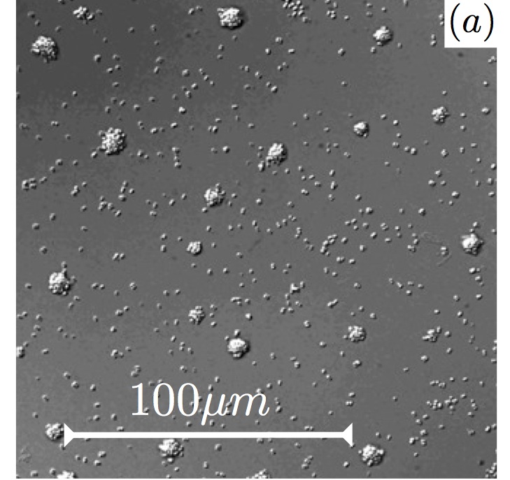
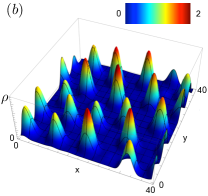
Figure 1: (color online) (a) N. gonorrhoeae colonies three hours after sedimentation on a plastic substrate. (b) Typical snapshot of state obtained from a numerical solution to Eq. (2) at large time scales.

However, so far, the physical mechanisms governing the formation and dissolution of bacterial colonies are poorly understood. Since motility and interactions are driven by active retractions of pili, fundamental concepts from equilibrium statistical mechanics are in general not applicable. The inherent non-equilibrium nature of this system suggests to consider a kinetic approach reminiscent of the Boltzmann equation, which has been successfully employed to describe the order-disorder transitions in several active systems far from equilibrium Aronson_MT ; Bertin_short ; Bertin_long ; Saintillan_2007 ; Aranson_Bakterien ; Saintillan_2008 ; Ihle_2011 ; Thuroff_2013 ; Weber_NJP_2013 ; Hanke_2013 ; prx_with_flo_2014 .

Here we propose a kinetic description as a general framework of how living colonies form and dissolve, which keeps track of the length scales and the specific properties of the interactions between individuals. By a coarse-graining procedure we derive the corresponding hydrodynamic equation and find an ordering instability for a choice of parameters relevant to N. gonorrhoeae. It belongs to a class of instabilities, where the diffusion constant is negative and originates from attractive pili-mediated interactions. As most of the parameters can be estimated based on available data for N. gonorrhoeae, we analytically compute the corresponding phase-diagram and the characteristic colony size that is consistent with experimental observations.

Our theory can also be used to compare the effects of different cell-cell interactions and investigate their interplay. We show that pili interactions are more effective regarding clustering than cell adhesion. Moreover, when both interactions keep the cells together in the colony, a more efficient and robust way to dissolve the colony is to lower the strength of pili-mediated interactions. This suggests that pili play an essential role not only in cell motility and assembly, but also in the dissolution of matured colonies. Our results demonstrate that kinetic theory can be applied to quantify the process of colony formation in living systems and is able to provide insights about the underlying physical mechanisms.

Kinetic Model: Our kinetic description is formulated in terms of the particle density $f(\mathbf{r},t)$. We restrict ourselves to two-dimensional colonies forming on a planar substrate , which do not give rise to swarms or swirls (see e.g. Aranson_Bakterien ). Therefore, the spatial coordinates $\mathbf{r}\in\mathbb{R}^{2}$ suffice as dynamical variables. In the absence of interactions cells are assumed to move across the substrate by pili-mediated displacements as in case of N. gonorrhoeae or N. meningitidis, leading to a diffusive behaviour at large length and time-scales Holz_2010 . Interactions enter the kinetic description via “collision rules”. A collision rule $\mathcal{R}$ maps the pre-collision coordinates to the post-collision positions by means of the delta-functions $\delta(\cdot)$. The corresponding kinetic equation is:

$$\partial_{t}f(\mathbf{r},t)=\mathcal{C}_{\text{mot}}(\mathbf{r},t)+\mathcal{C}_{\text{int}}(\mathbf{r},t),$$ (1a)

where $$\mathcal{C}_{\text{mot}}$$ describes the cell motility across the substrate

$$\mathcal{C}_{\text{mot}}(\mathbf{r},t)=\int\text{d}\mathbf{r}^{\prime}\left[\mathcal{K}_{\mathbf{r}^{\prime}\to\mathbf{r}}f(\mathbf{r}^{\prime},t)-\mathcal{K}_{\mathbf{r}\to\mathbf{r}^{\prime}}f(\mathbf{r},t)\right]$$ (1b)

and $$\mathcal{C}_{\text{int}}$$ accounts for the cell-cell interactions

$$\mathcal{C}_{\text{int}} (\mathbf{r},t)=\frac{1}{2}\int\text{d}\mathbf{r}_{1}\int\text{d}\mathbf{r}_{2}\,\mathcal{W}(|\mathbf{r}_{12}|)f(\mathbf{r}_{1},t)f(\mathbf{r}_{2},t)$$

$$\times \left[\delta\left(\mathcal{R}_{1}(\mathbf{r}_{1},\mathbf{r}_{2})-\mathbf{r}\right)+\delta\left(\mathcal{R}_{2}\left(\mathbf{r}_{1},\mathbf{r}_{2}\right)-\mathbf{r}\right)-2\delta\left(\mathbf{r}_{2}-\mathbf{r}\right)\right].$$

$$\mathcal{K}_{\mathbf{r}\to\mathbf{r}^{\prime}} \mathbf{r} \mathbf{r}^{\prime} \ell_{\text{pi}} \mathcal{K}_{\mathbf{r}\to\mathbf{r}+\mathbf{b}}=\mathcal{K}_{0}/(2\pi\ell_{\text{pi}}^{2})\exp{\left(-|\mathbf{b}|/\ell_{\text{pi}}\right)} \mathcal{K}_{0} \mathbf{b}=\mathbf{r}^{\prime}-\mathbf{r}$$ denotes the transition kernel to move from to by a retraction event of an individual pilus. We assume that retraction events are independent and that the corresponding rate is isotropic, with a characteristic length scale given by the pili length . There is experimental evidence that the pili lengths are distributed exponentially Holz_2010 . Therefore, we consider for the transition kernel , with denoting the attachment rate of pili to the substrate and is the displacement resulting from an individual pilus retraction.

$\mathcal{W}(|\mathbf{r}_{12}|)$ characterizes the isotropic kernel for collisions between cells with $|\mathbf{r}_{12}|=|\mathbf{r}_{1}-\mathbf{r}_{2}|$ denoting the relative cell-cell distance. For pili-mediated attractive displacements, we consider the following collision rule:

$$\left(\mathbf{r}_{1},\mathbf{r}_{2}\right)\rightarrow\left(\mathcal{R}_{1},\mathcal{R}_{2}\right)=\left(\mathbf{r}_{1}-a\mathbf{r}_{12},\mathbf{r}_{2}+a\mathbf{r}_{12}\right),$$ (1d)

where $a\in[0,1/2]$ is a measure for the strength of the attractive interaction. For $a=1/2$, cells are maximally attracted and displaced to the center-of-mass coordinate $\mathbf{R}_{12}=\left(\mathbf{r}_{1}+\mathbf{r}_{2}\right)/2$ between the collision partners, while for $a=0$, cells diffuse freely without interacting. Due to the exponential distribution of the pili lengths, the interaction rate is $\mathcal{W}_{\text{pi}}(|\mathbf{r}_{12}|)=\gamma\mathcal{W}_{0}/(2\pi\ell_{\text{pi}}^{2})\exp{\left(-|\mathbf{r}_{12}|/\ell_{\text{pi}}\right)}$, where $\ell_{\text{pi}}$ sets the characteristic length scale for the attractive interaction and $\mathcal{W}_{0}$ denotes the interaction rate. Since pili-mediated cell-cell interactions are intrinsically stochastic Rahul_Klumpp_2014 ; vasily_dave_2014 , we introduce a non-dimensional number, $\gamma$, accounting for the number of successful binding and retraction events to the total number of pili-cell encounter events.

Coarse-graining: The isotropy of the interaction rates allows us to integrate Eq. (1) over the center-of-mass coordinates $\mathbf{R}_{12}$ leading to non-local terms (see Supplemental Material SM , S1). These terms are related to the length scales of the interactions and resemble a phenomenological description for the assembly of active bundles Kruse_2000 ; Kruse_2003a ; Kruse_2003b . Since cell colonies typically exhibit sizes noticeably beyond the interaction length scale, the non-local integrands can be removed by expanding the particle density $f$ with respect to the spatial coordinates Aronson_MT ; Aranson_Bakterien . Truncation of this expansion amounts to coarse-graining beyond the interaction length scale. To obtain a well-defined set of hydrodynamic equations for the dynamics of bacterial colonies with pili-mediated interactions we truncate at the fourth order (see Supplemental Material SM , S2):

$$\partial_{t}\rho(\mathbf{r},t) = \alpha(\rho)\nabla^{2}\rho(\mathbf{r},t)-\beta_{1}\,|\nabla\rho(\mathbf{r},t)|^{2}+\kappa(\rho)\,\nabla^{4}\rho(\mathbf{r},t)$$ (2)

$$+ \beta_{2}\,\left[\nabla^{2}\rho(\mathbf{r},t)\right]^{2}-\beta_{3}\,\left[\nabla\rho(\mathbf{r},t)\right]\cdot\nabla^{3}\rho(\mathbf{r},t),$$

where $\rho=f\cdot\ell_{\text{pi}}^{2}$ is the dimensionless density and the kinetic coefficients are

$$\alpha(\rho) = G-\beta_{1}\,\rho(\mathbf{r},t),$$ (3)

$$\kappa(\rho) = -\left(\beta_{2}+\beta_{3}\right)\,\rho(\mathbf{r},t),$$ (4)

$\beta_{1}=a\bar{a}\tilde{c}_{2}$, $\beta_{2}=a^{2}\bar{a}^{2}\tilde{c}_{4}/4$, $\beta_{3}=\left(a\bar{a}^{3}+\bar{a}a^{3}\right)\tilde{c}_{4}/6$; $\bar{a}=1-a$. Note that all $\beta_{i}>0$. The numerical constants $\tilde{c}_{k}$ are given in the Table of the Supplemental Material SM . In Eq. (2), we rescaled coordinates by the pili length $\ell_{\text{pi}}$, i.e. $\mathbf{r}\to\mathbf{r}\cdot\ell_{\text{pi}}$, leading to a rescaling of time
$t\to t\cdot\ell_{\text{pi}}^{2}/(\mathcal{W}_{0}\gamma)$. We introduce the dimensionless parameter, $G=D/(\gamma\mathcal{W}_{0})$, with $D=3\mathcal{K}_{0}\ell^{2}_{\text{pi}}$ denoting the single cell diffusion constant. $G$ is reminiscent of the inverse Péclet number and can be interpreted as a measure for the rate of diffusive particle transport relative to the frequency of interactions. In other words, given a time period between two successive collisions, $G$ quantifies how much distance is traveled (on average) by diffusion with respect to the mean free path.

A equation similar to Eq. (2) but phenomenologically constructed appeared in the context of laminar flames and propagation of concentration waves referred to as Kuramoto-Sivashinsky equation Kuramoto01021976 ; Sivashinsky . It has also been pointed out as an appropriate framework to study instabilities in growing yeast colonies PhysRevLett.79.313 . However, Eq. (2) is distinctively different because the kinetic coefficients depend on density [Eqs. (3) and (4)]. Moreover, Eq. (2) exhibits an alleged similarity to the Cahn-Hilliard equation studied in the context of liquid-liquid demixing Bray_Review_1994 . Though both equations have terms of similar orders in $\mathcal{O}(\nabla\rho)$, they are fundamentally different with respect to the saturation of droplet or colony growth. The Cahn-Hilliard equation exhibits an instability of the homogeneous state, which saturates because the effective diffusion constant in front of the LaPlace operator decreases to zero. Eq. (2) also exhibits an instability but it saturates due to a different mechanism as discussed below.

Colony formation due to pili-mediated interaction: The condition for the instability in Eq. (2) is $\alpha(\rho)<0$. Its onset marks a critical density, $\rho_{\text{c}}=G/\beta_{1}$. For $\rho_{0}>\rho_{\text{c}}$, the homogenous state of density $\rho_{0}$ is unstable. The instability enhances small density modulations around the homogenous density $\rho_{0}$ with a dispersion relation $w(q)=-\alpha(\rho_{0})q^{2}-\kappa(\rho_{0})q^{4}$. $\rho_{\text{c}}$ depends on the non-dimensional parameter $G$ and the interaction strength $a$, $\rho_{\text{c}}=G/(a\bar{a}\tilde{c}_{2})$. We find that $\rho_{\text{c}}$ decreases for stronger attractive interactions,  $a\to 1/2$, and smaller values of $G$; see Fig. 2(a,b).

The instability is opposed by fluxes related to the spatial curvature of the density field, which can be qualitatively understood by splitting the flux, $\mathbf{j}=\mathbf{j}_{\text{inst}}+\mathbf{j}_{\text{cu}}+\mathbf{j}_{\nabla\text{cu}}$ with $\partial_{t}\rho=-\nabla\cdot\mathbf{j}$. $\mathbf{j}_{\text{inst}}=-\alpha(\rho)\nabla\rho$ denotes the ‘instability flux’ which acts for $\alpha<0$ like negative diffusion thus driving particles to the center of a density spot [see Fig. 2(c) for an illustration]. There the instability current is opposed by the ‘curvature flux’, $\mathbf{j}_{\text{cu}}=-\beta_{2}(\nabla^{2}\rho)\nabla\rho$, and the ‘gradient-curvature flux’, $\mathbf{j}_{\nabla\text{cu}}=(\beta_{2}+\beta_{3})\rho\nabla(\nabla^{2}\rho)$. Both are directed outwards of the density spot since curvature is negative and increases.

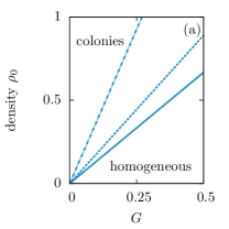
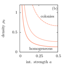
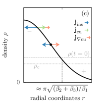
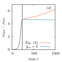
Figure 2: (color online) (a,b) Critical density $\rho_{\text{c}}$ as a function of the non-dimensional parameter $G$ and interaction strength $a$. Each line separates the parameter space, where colonies develop or the system remains homogeneous. In (b), three values of interaction strength $a$ are displayed: $(0.5,0.25,0.1)$ =(solid, dashed, dash-dotted), and (c) depicts three values of $G$: $(0.1,0.2,0.5)$=(solid, dashed, dash-dotted). (c) Illustration of how the instability is balanced: For initial densities $\rho(t=0)>\rho_{\text{c}}$, the ‘instability flux’ $\mathbf{j}_{\text{ins}}$ drives the emergence of a spatially inhomogeneous density profile. Depending on the location along the density profile, the ‘curvature flux’ $\mathbf{j}_{\text{cu}}$ and/or the ‘gradient curvature flux’ $\mathbf{j}_{\nabla\text{cu}}$ acts against the ‘instability flux’ $\mathbf{j}_{\text{ins}}$ and thereby balances the instability. (d) Maximal density minus minimal density, $\rho_{\text{max}}-\rho_{\text{min}}$, as a function of time $t$, where $\rho_{\text{max}}(t)=\text{max}_{\mathbf{r}}\rho(\mathbf{r},t)$ and $\rho_{\text{min}}(t)=\text{min}_{\mathbf{r}}\rho(\mathbf{r},t)$, for numerical solutions to Eq. (2) with and without ‘curvature flux’ $\mathbf{j}_{\text{cu}}$.

Our findings on the instability and its saturation can be scrutinized by numerically solving Eq. (2). A representative snapshot of a state at large time-scales is shown in Fig. 1(b), which appears to be similar to N. gonorrhoeae colonies three hours after sedimentation on a plastic substrate [Fig. 1(a)]. Using parameter values consistent with the experimental system we observe multiple colonies developing quickly for densities above the critical value. We checked numerically that for all parameter values lying within the ‘colony phase’ of the analytic phase diagram [Fig. 2(a,b)] give rise to the formation of colonies. After the onset of the instability, colonies exponentially grow with a growth speed that is higher the larger the difference of the homogeneous density $\rho_{0}$ to the critical density $\rho_{\text{c}}$; see Supplemental Material SM , S.4. Thus, for $\rho_{0}\searrow^{+}\rho_{\text{c}}$, we observe a colony growth rate decreasing to zero; a phenomena reminiscent of ‘critical slowing down’ in phase transitions Onuki_book . Subsequent to the initial growth, there is regime, where colonies grow only very slowly [Fig. 2(d), solid red line]. The later observation is due to a weak interaction between the colonies via some evaporation-condensation mechanism qualitatively reminiscent of Ostwald-ripening in liquid-liquid phase-separation Bray_Review_1994 . Interestingly, at the onset of the instability the non-linear ‘curvature flux’ $\mathbf{j}_{\text{cu}}$ vanishes suggesting that it might play an essential role for developed colonies at large time-scales. Running the system without curvature flux, $\mathbf{j}_{\text{cu}}=0$, we find that the subsequent ripening is absent leading to a stable state consisting of multiple colonies [see Fig. 2(d), dashed line]. This implies that interactions between colonies is driven by the ‘curvature flux’, while the ‘gradient curvature flux’ suffices for the saturation. Based on this insight we can analytically estimate the colony size at the time when the system crosses to the very slow ripening regime [vertical line in Fig. 2(d)] by neglecting the curvature flux (see Supplemental Material SM , S.3 for more details). For densities $\rho\gg\rho_{\text{c}}$, stationary periodic solutions are supported with the quasi-static colony size of $\pi\sqrt{(\beta_{2}+\beta_{3})/\beta_{1}}$. Remarkably, for $a=0.5$, this estimate suggests a colony size of several pili-lengths, which is consistent with N. gonorrhoeae [Fig. 1(a)].

Biological relevance: In principle, all parameters entering the kinetic description Eq. (1) can be measured or estimated for living colonies forming on a substrate and thereby all kinetic coefficients in Eq. (2). In particular, for N. gonorrhoeae, $\ell_{\text{pi}}\approx 1\mu m$ Holz_2010 ; vasily_dave_2014 and colony formation is observed for densities of $\rho\approx 0.2$. The attachment rate to the substrate can be obtained from measurements of the single cell diffusion constant, $\mathcal{K}_{0}=D/(3\ell_{\text{pi}}^{2})\approx(6s)^{-1}$ with $D\approx 0.5\mu m^{2}/s$ Taktikos_2014 and the cell-cell interaction rate can be roughly estimated from the experimental value of the mean next neighbour distance and the mean pili-number per cell to $\mathcal{W}_{0}/\ell_{\text{pi}}^{2}\sim 5s^{-1}$ (see Supplemental Material SM , S7). Therefore, a typical value for the dimensionless parameter for N. gonorrhoeae is $G\sim 0.1\gamma^{-1}$. Recently, the attachment probability of pili to a substrate has been determined by fitting a model to experimental results vasily_dave_2014 , finding an approximate value of $0.5$. We expect a roughly similar, maybe lower value for $\gamma$ since successful binding to another cell can be hindered by other moving cells. So far an appropriate estimate for the interaction strength $a$ is missing because the synchronous visualization of pili and cell movement is not feasible for large enough time-scales. Thereby, we consider $a$ as an unknown parameter.

The proposed kinetic description, Eq. (1), can also be used to include other attractive interactions such as adhesion. Since cell-cell adhesion constitutes a local interaction on the scale of the cell diameter, an appropriate weight function is for example a Gaussian of the form $\mathcal{W}_{\text{ad}}(|\mathbf{r}_{12}|/\ell_{\text{ad}})=\mathcal{W}_{0}/(\pi\ell_{\text{ad}}^{2})\exp{\left(-\mathbf{r}_{12}^{2}/\ell_{\text{ad}}^{2}\right)},$ where $\ell_{\text{ad}}$ denotes the characteristic length scale which is in the order of the cell size. Comparing both interactions (see Supplemental Material for details SM , S.5) we find that pili allow for a significantly more pronounced affinity for colony formation compared to adhesive interactions, i.e. colonies already form at smaller initial density of cells.

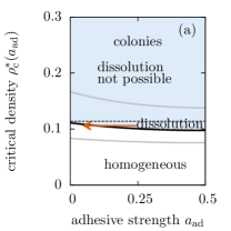
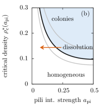
Figure 3: (color online) Critical density $\rho^{*}_{\text{c}}(a_{\text{ad}},a_{\text{pi}})/G$ as a function of (a) adhesive strength $a_{\text{ad}}$ (with $a_{\text{pi}}=0.5$) and (b) pili-mediated interaction strength $a_{\text{pi}}$ (with $a_{\text{ad}}=0.5$). In both plots, $G=0.1$ and each solid line corresponds to $\gamma\in\{0.4,0.3,0.2\}$ from top to bottom. Black line corresponds to $\gamma=0.3$. The horizontal black dashed line (plotted only for $\gamma=0.3$ in (a)) marks the dissolution boundary: Below, dissolution (red arrow) is possible, above not. Blue shaded areas correspond to the “colony-phase”.

Colony dissolution: Many bacteria are known to interact simultaneously by adhesion and pili. It is hypothesized that these bacteria are able to switch off either adhesion or the pili-mediated interaction without affecting their ability to move  Chamot-Rooke11022011 ; EMI:EMI775 ; Gcell_dissolution_Maier_2015 . Now we address the question of whether developed colonies can dissolve by switching off either one of these interactions. In other words, given the phase-diagram of a specific bacteria system, we discuss some possible means of leaving the “colony-phase” by $a_{\text{pi}}\to 0$ or $a_{\text{ad}}\to 0$. We now include both interactions by adding a term for pili-mediated interactions $\mathcal{C}_{\text{int,pi}}$ and a term corresponding to adhesive interactions $\mathcal{C}_{\text{int,ad}}$ on the right hand side of Eq. (1a), i.e. $\mathcal{C}_{\text{int}}=\mathcal{C}_{\text{int,pi}}+\mathcal{C}_{\text{int,ad}}$. In addition to the already introduced different length scales $\ell_{\text{pi}}$ and $\ell_{\text{ad}}$, we also distinguish the corresponding interaction strengths, denoted as $a_{\text{pi}}$ and $a_{\text{ad}}$ (values for adhesion and pili-mediated interactions are denoted as $\tilde{c}_{k,\text{ad}}$ and $\tilde{c}_{k,\text{pi}}$). We rescale coordinates, density and time by the adhesive interaction length $\ell_{\text{ad}}$ (or cell size), i.e. $\mathbf{r}\to\mathbf{r}\cdot\ell_{\text{ad}}$, $f\to f/\ell_{\text{ad}}^{2}\equiv\rho$ and $t\to t\cdot\ell_{\text{ad}}^{2}/\mathcal{W}_{0}$, thereby introducing a ratio of these length scales, $\epsilon=\ell_{\text{pi}}/\ell_{\text{ad}}$. For the case where cells interact with both adhesive and pili-mediated interactions, we find the following effective diffusion constant (further coefficients see Supplemental Material SM , S6): $\alpha(\rho)=G-\rho\,\left[a_{\text{ad}}\bar{a}_{\text{ad}}\,\tilde{c}_{2,\text{ad}}+a_{\text{pi}}\bar{a}_{\text{pi}}\,\tilde{c}_{2,\text{pi}}\,\gamma\,\epsilon^{2}\right]$. Setting this equation equal to zero marks a critical density $\rho^{*}_{\text{c}}(a_{\text{ad}},a_{\text{pi}})=G/\left[a_{\text{ad}}\bar{a}_{\text{ad}}\,\tilde{c}_{2,\text{ad}}+a_{\text{pi}}\bar{a}_{\text{pi}}\,\tilde{c}_{2,\text{pi}}\,\gamma\,\epsilon^{2}\right]$ depending on the strength of both interactions, $a_{\text{ad}}$ and $a_{\text{pi}}$.

In order to study the impact of both interactions for dissolution of colonies we choose the parameters ($\epsilon$, $\gamma$) relevant to N. gonorrhoeae. Fig. 3(a) shows $\rho^{*}_{\text{c}}(a_{\text{ad}})$ as a function of $a_{\text{ad}}$ for $a_{\text{pi}}=0.5$ and $G=0.1$, while Fig. 3(b) depicts $\rho^{*}_{\text{c}}(a_{\text{pi}})$ as a function of $a_{\text{pi}}$ for $a_{\text{ad}}=0.5$ and $G=0.5$, both for several values of $\gamma$. For a given $\gamma$, there are two qualitatively distinct regimes for the case where adhesive interactions are switched off [Fig. 3(a)]: For small enough $\rho^{*}_{\text{c}}$ below the “dissolution boundary” (horizontal dashed line), colonies can dissolve by switching off the adhesive interaction ($a_{\text{ad}}\to 0$) and is indicated by the red arrows. However, above the dissolution boundary, colonies cannot dissolve. Interestingly, choosing the parameters relevant to N. gonorrhoeae gives a rather small density regime, where colonies can dissolve, rendering the dissolution scenario through switching off adhesion as a non-robust mechanism. This is in stark contrast to the scenario of switching off pili-mediated interactions [Fig. 3(b)]: For a given $\gamma$, dissolution is possible for all experimental densities in the “colony-phase” by lowering the pili-interaction strength, $a_{\text{pi}}\to 0$. These findings suggest that switching off pili-mediated interactions is a more robust mechanism for the dissolution of bacterial colonies than switching off adhesion.

To summarize, the formation of living colonies is investigated using a hydrodynamic equation derived from a kinetic description, where most of the parameters can be estimated from experimental data for N. gonorrhoeae bacteria. Our results demonstrate that kinetic theory can be successfully used to describe complex far from equilibrium systems such as formation and dissolution of living bacterial colonies. Applications of this theory could pave the way for the physical quantification of the initial stages of biofilm formation. Though biological reasons for colony formation are specific to each system there are qualitative similarities Ben-Jacob_review_1998 ; Lejeune_2002 ; Higashi_2007 ; Taktikos_2014 ; biofilm_review_2014 ; PhysRevLett.79.313 : Colonies form due to encounters with nearby individuals giving rise to structures of a characteristic size determined by the intra-species interactions and the environment. These similarities suggest that our kinetic description might be applied to other colony-forming systems while the kinetic coefficients in the resulting hydrodynamic equation may differ for each system. Further open questions concern the role of cell division and stochastic fluctuations in living colonies Tsimring_review_noise_biology_2014 .

See pages 1 of Supplement_Kinetic_description_formation_and_dissolution_of_bacteria_cononies.pdf See pages 2 of Supplement_Kinetic_description_formation_and_dissolution_of_bacteria_cononies.pdf See pages 3 of Supplement_Kinetic_description_formation_and_dissolution_of_bacteria_cononies.pdf See pages 4 of Supplement_Kinetic_description_formation_and_dissolution_of_bacteria_cononies.pdf See pages 5 of Supplement_Kinetic_description_formation_and_dissolution_of_bacteria_cononies.pdf