Phase ordering in disordered and inhomogeneous systems

Abstract

We study numerically the coarsening dynamics of the Ising model on a regular lattice with random bonds and on deterministic fractal substrates. We propose a unifying interpretation of the phase-ordering processes based on two classes of dynamical behaviors characterized by different growth-laws of the ordered domains size - logarithmic or power-law respectively. It is conjectured that the interplay between these dynamical classes is regulated by the same topological feature which governs the presence or the absence of a finite-temperature phase-transition.

I Introduction

When a ferromagnetic system is quenched to below the critical temperature a slow non-equilibrium phase-ordering process takes place with domains of the ordered phases increasing their size $L(t)$ in time bray ; 2dinoirf . Typical examples are ferromagnets, binary liquids or alloys. When time is large, due to the presence of the dominant length scale $L(t)$ dynamical scaling sets in zan ; BCKM ; ioeleti . The main features of this structure, which is quite well understood in non-disordered homogeneous systems, is expected to be valid also in the presence of quenched disordered or when homogeneity is spoiled. Recently, this has promoted a considerable effort to understand coarsening phenomena in disordered and in non-homogeneous systems diluted ; sab08 ; puripowerlaw ; super2 ; hp06 ; lastparma ; super3 ; decandia ; EPL ; CLMPZ ; variousnoi2 ; various2 ; super1 ; 10noirf ; pp ; HH ; parma . Particular attention was devoted to the asymptotic growth law since, although a logarithmic behavior was generally expected, also a power-law sometimes was reported puripowerlaw ; super2 ; hp06 .

In a recent paper diluted some of us have studied a system - the site diluted Ising model (SDIM) - where, the interplay between logarithmic and power-law growth can be fully understood and the occurrence of the two types of behavior can be tuned by means of the amount of dilution. In the site diluted model Ising spins are located on a substrate which is obtained from a regular lattice by removing randomly a fraction $D$ of sites. In the pure case with $D=0$, the usual temperature-independent power-law $L(t)\sim t^{1/z}$ is obeyed, where $z=2$ for a dynamics without conservation of the order parameter, as it will be considered here. Increasing $D$, a region with an asymptotic logarithmic behavior of $L(t)$ is entered. However the situation changes when the critical value $D=D_{c}$ is reached, such that the fraction $P_{c}=1-D_{c}$ of spins is at the percolation threshold. In this case a temperature-dependent power-law $L(t)\sim t^{1/\zeta(T)}$ is observed. This is interpreted as due to the different topology of the substrate, for $D<D_{c}$ and for $D=D_{c}$, since in the former case it is compact on large scales, while in the latter it is a percolation fractal. Notice that the critical temperature $T_{c}$ of the model, which is finite for $D<D_{c}$, vanishes at the percolation threshold $D=D_{c}$.

The role of the substrate topology was also explored, in a different context, in lastparma where the coarsening of the Ising model defined on deterministic fractal networks was considered. There it was shown that, again, two types of growth, logarithmic versus temperature dependent power-law, could be observed depending on the substrate considered. In particular, it was argued that logarithmic behavior is found on networks with a finite Ising critical temperature, while temperature-dependent power laws are observed on structures with $T_{c}=0$.

The above findings suggest that the substrate topology, which is responsible for the existence of the equilibrium phase-transition, might also be important in determining the non-equilibrium growth-law, leading to the conjecture that temperature-dependent power-laws are to be expected on inhomogeneous or disordered systems with $T_{c}=0$ - like the SDIM at the percolation threshold - while a logarithmic behavior occurs when $T_{c}>0$, as in the same model with $D<D_{c}$.

In the above mentioned cases, the Ising model is constructed on a substrate with topological properties obtained by diluting the lattice either randomly or according to a deterministic rule. Other thoroughly studied systems such as the Ising model with random bonds or random fields are defined on homogeneous lattices. In these cases disorder pins the interfaces whose evolution becomes site-dependent and the growth-law is observed to be much slower than in the corresponding pure systems decandia ; EPL ; CLMPZ ; variousnoi2 .

In this Article, by studying an asymmetric version of the random-bond Ising model, we argue that this is the case. We explicitly exhibit the parameters controlling the speed of growth and set them as to produce either a faster or a slower asymptotic growth law which are well compatible with an algebraic or a logarithmic behavior. These parameters have a clear geometrical interpretation in terms of topological properties of the bond network and, accordingly, one finds logarithmic or temperature-dependent power-law growths. Our results hint to promote the relation between topology and growth-law to a general feature of inhomogeneous and/or disordered phase-ordering systems.

The paper is organized as follows. The random bond model is defined in Sec. II. Numerical simulations are discussed in Sec. III. In order to better understand the role of topology, a pair of systems with Ising spins on deterministic fractal substrates are introduced in Sec. IV. The study of these models allows to gain useful qualitative insights into the more complicated random bond system. Finally, some open issues are briefly discussed in the concluding Sec. V.

II The asymmetric Random Bond Ising Model

We consider an Ising model, hereafter referred to as the asymmetric random-bond Ising model (ARBIM) which is described by the following Hamiltonian

$$H=-\sum_{<ij>}J_{ij}\sigma_{i}\sigma_{j}.$$ (1)

Here $\sigma_{i}=\pm 1$ are spins on a 2-d square lattice, $<ij>$ are nearest neighbors and $J_{ij}=J_{0}+\xi_{ij}$ are positive coupling constants. The $\xi_{ij}$ are uncorrelated random variables that can take two values $\pm\epsilon$, with $\epsilon\leq J_{0}$ to ensure the positivity of $J_{ij}$. The probability of occurrence $P(\xi_{ij})$ of the two possible values $\xi_{ij}=\pm\epsilon$ is assumed to be in general asymmetric with $P(\xi_{ij}=-\epsilon)=d$. In order to be concrete, let us make the example of a case which will be important in the following, with $\epsilon=J_{0}$. This situation corresponds to a model with random coupling constants bi-modally distributed on the two possible values $J_{ij}=0$ and $J_{ij}=2J_{0}$ occurring with probability $d$ and $1-d$, respectively. Therefore, this case corresponds to the Ising model with $J_{ij}=2J_{0}$ and bond dilution, namely with a fraction $d$ of the bonds removed.

II.1 Space of parameters

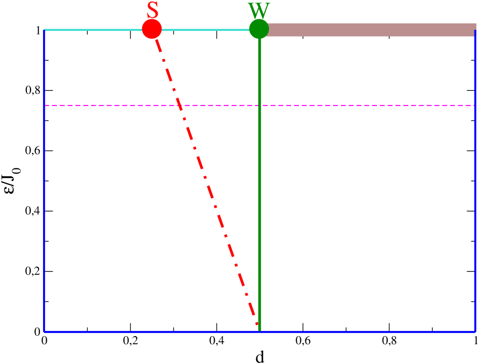
Figure 1: (Color online). Parameter space of of the model. The blue lines on the left, right and bottom of the figure correspond to a pure system. Red and green heavy dots are the strong-disorder (S) and percolative (W) fixed points with $\epsilon=J_{0}$. Dot-dashed red and continuous green heavy lines are the line of fixed points originating from S and W upon changing $\epsilon$ (see Secs. III.2,III.3).

In the limit of low temperatures that we will always consider in this paper, the model depends only on $d$ and $\epsilon$. In the parameter space, sketched in Fig. 1, only the region with $0\leq d\leq 1$, $0\leq\epsilon/J_{0}\leq 1$ is allowed since $d$ is a probability and because we limit our analysis to non-negative coupling constants in order to avoid the different problem where frustration occurs (notice that we use $\epsilon/J_{0}$ on the diagram axis instead of $\epsilon$).

In Fig. 1 the axes with $d=0$, $d=1$, and $\epsilon=0$ correspond to the pure Ising model (i.e. there is no disorder in the couplings). This is pictorially represented by drawing them in blue.

The point $d=1/2,\epsilon/J_{0}=1$, hereafter referred to as $W$, will be particularly relevant in the following since, recalling the discussion above, it can be regarded as a system with uniform couplings $J_{ij}\equiv 2J_{0}$ but where a fraction $d=d_{c}=1/2$ of the bonds has been randomly removed. Since $p_{c}=1-d_{c}=1/2$ is the bond percolation threshold, the system is at the percolation point of the substrate. Let us recall here that the Ising model defined on this percolative network is characterized by $T_{c}=0$. This is due to the presence of the so called cutting bonds Stauffer , namely isolated bonds whose removal would cause the disconnection of arbitrarily large parts of the structure. In this sense the network is weak and we denote this point with the letter $W$. Notice that the region with $\epsilon/J_{0}=1,d>d_{c}$, represented in brown in Fig. 1, is not interesting since on that sector the substrate is disconnected and asymptotic phase-ordering cannot occur.

II.2 Time Evolution

We implement non-conserved dynamicsbray ; 2dinoirf by evolving the spins with a single-spin-flip transition rates of the Glauber form

$$w(\sigma_{i}\to-\sigma_{i})=\frac{1}{2}\left[1-\sigma_{i}\tanh(H_{i}^{W}/T)\right].$$ (2)

Here, $H_{i}^{W}$ is the local Weiss field obtained by the sum

$$H_{i}^{W}=\sum_{j\in L_{i}}J_{ij}\sigma_{j}$$ (3)

over the set of nearest-neighbors $L_{i}$ of $i$.

Before presenting numerical simulations, in the next section we briefly overview the behavior of the closely related site diluted model.

II.2.1 The segment $\epsilon=J_{0}$ and the relation with the site diluted model

It is useful to stress the close relation between the segment $\epsilon/J_{0}=1$, $0\leq d\leq d_{c}$ of the present model and the SDIM studied in diluted . The latter has a fixed coupling constant but a fraction of spins is randomly removed with a probability $D$ (we use capital $D$ to distinguish it from the ARBIM disorder parameter $d$). ARBIM with $\epsilon/J_{0}=1$ differs from SDIM because of bond dilution in place of site dilution. Since we expect similar properties for the two systems it is useful to overview first the behavior of the SDIM. In this model the dilution parameter can be varied between $D=0$, corresponding to the pure Ising model, up to $D_{c}=1-P_{c}$, where $P_{c}\simeq 0.5928$ is the site percolation threshold. For $D>D_{c}$ the substrate is disconnected and asymptotic coarsening cannot occur, not differently from the ARBIM for $d$ above $d_{c}$.

In Ref.diluted it was shown that the SDIM kinetic properties display a scaling structure which is most effectively described in terms of three competing fixed points on the $D$ axis, making free use of renormalization group terminology. The first is the trivial one of the pure system, located at $D=0$, and is associated to the usual power-law growth $L(t)\sim t^{1/2}$. The second one is the percolative fixed point located at $D_{c}$ and is characterized by a temperature-dependent power-law growth $L(t)\sim t^{1/\zeta(T)}$. These fixed points are repulsive, in the sense that as soon as $D>0$, or $D<D_{c}$ the asymptotic dynamics is governed by a different fixed point, located at $D=D^{*}\simeq 0.225$, to whom a logarithmic increase of $L(t)$ is associated. Due to this fixed point structure, if the system is prepared with an intermediate dilution between $D=0$ and $D^{*}$ (or equivalently between $D^{*}$ and $D_{c}$) a crossover is observed at a certain time $t_{cross}(T,D)$ from an initial transient regime governed by the nearest unstable fixed point ($D=0$ or $D_{c}$ respectively), with a power-law increase of the domains size, to a late regime controlled by the attractive point at $D^{*}$, characterized by a logarithmic $L(t)$. As a result, the slowest possible growth, namely the one where $t_{cross}(T,D)$ is smallest, is obtained at $D=D^{*}$ and comparing $L(t)$ for different values of $D$ one finds a non-monotonous behavior: The growth slows down in going from $D=0$ to $D=D^{*}$ and then speeds up again when $D$ is further increased from $D=D^{*}$ up to $D=D_{c}$. This can be used as a practical way to identify $D^{*}$.

Since the only difference between the ARBIM with $\epsilon/J_{0}=1$ and the SDIM is bond dilution replacing site dilution, we expect to observe the same pattern with an attractive fixed point associated to logarithmic growth and located somewhere in between $d=0$ and $d=d_{c}$. This is represented in Fig. 1 by the heavy red dot marked with the letter $S$, corresponding to the dilution $d=d^{*}$. For this value of $d$ the growth-law is expected to be the slowest possible one, in the sense discussed above. Evidence for the existence of this fixed point will be discussed in Sec. III.

III Numerical simulations

We have performed a series of simulations of the ARBIM by considering a cooling procedure where the system is prepared initially in the infinite-temperature disordered state and, at the time $t=0$, it is suddenly quenched to a finite temperature $T$. If not specified differently we use $T=\epsilon$. This temperature is chosen as a compromise between the aim of studying the low temperature sector, where dynamical properties can be better interpreted, and the severe limits posed by the slowing down of the dynamics for $T\to 0$.

In order to speed up simulations we have used a modification of the dynamics introduced in Sec. II.2 where flipping spins in the bulk of domains, namely those aligned with all the nearest neighbors, is prevented. This modified dynamics does not alter the behavior of the quantities we are interested in, as it has been tested in a large number of cases nobulk ; Ontheconnec ; diluted . We have checked that this is true also in the present study.

In our simulations we have used sufficiently large system sizes in order not to have any detectable finite-size effect in the range of time accessed in the runs. Specifically, we have considered a two-dimensional square lattice of $N={\cal L}^{2}$ sites with ${\cal L}$ in the range $[10^{3}-2\cdot 10^{3}]$ for quenches in different sectors of the parameter space of Fig. 1. For every choice of the parameters, we have performed a certain number (in the range 10-100) of independent runs with different initial conditions and thermal histories in order to populate the non-equilibrium ensemble needed to extract the average quantities that will be introduced below.

The observable of interest in this paper is the typical domains size $L(t)$. In homogeneous systems this quantity is trivially related by

$$L(t)=e^{-1}(t)$$ (4)

to the excess energy density

$$e(t)=\frac{1}{V}[<H(t)>-<H>_{f}],$$ (5)

where $<H>_{f}$ is the average energy of the equilibrium state at the final temperature of the quench. Eq. (4) simply states that the excess energy is stored on the interfaces whose density scales as the inverse of the size of the growing domains bray .

In the model considered here the substrate can have disconnected parts. This happens, for instance, for $\epsilon=J_{0}$ and sufficiently large values of $d$. In this case phase ordering occurs independently and with different characteristics on the various parts of the system and, correspondingly, different definitions of the growing length can be given. Let us consider the case $\epsilon=J_{0}$, $d=1/2$, where the substrate if formed by an infinite spanning cluster and many finite-size parts. Since we are interested in the aging phenomenon related to the existence of a divergent length, one would define $L(t,d)$ as the characteristic length of the ordered regions which are effectively growing. Keeping in mind the example with $\epsilon=J_{0}$ one can argue that the quantity (4) introduced before is suited to the task. Indeed, at any given time there will be a number of sufficiently small disconnected parts of the substrate which are already ordered. These pieces of the system do not contribute to the computation of $L(t,d)$ in Eq. (4), because a finite cluster is by definition surrounded by bonds with $J_{ij}=J_{0}=\epsilon=0$ and hence there is no excess energy associated with it when its inner spins are aligned. For this reason in this paper we use the determination (4) of $L(t)$. A discussion of the relation between Eq. (4) and other possible definitions of L(t) in non-homogeneous systems can be found in Ref. diluted .

In the following we will describe the behavior of the ARBIM in different regions of the parameter space.

III.1 $\epsilon=J_{0}$

We start by investigating the line $\epsilon/J_{0}=1$, by varying $d$. This corresponds to scan the segment represented in turquoise in Fig. 1. As discussed in Sec. II.2.1 in this region of the parameter space we expect to see a behavior analogous to that observed in the SDIM. Specifically, as the parameter $d$ is varied, one should observe power-laws for $L(t)$ when $d$ is set to the limiting values $d=0$ and $d=d_{c}=1/2$, a logarithmic behavior for a certain value $0<d^{*}<d_{c}$, and a crossover from power-law to logarithm for intermediate values of $d$. Hence, comparing $L(t)$ for different values of $d$ a non-monotonous behavior is expected, with a faster growth at $d=0$ progressively slowing down upon approaching $d=d^{*}$, and then speeding up again in going from $d=d^{*}$ to $d=d_{c}$.

As shown in the left panel of Fig. 2 this is precisely what one observes in the ARBIM. Notice that here and in the following, in order to better compare the asymptotic behavior of $L(t)$ as the parameters are changed we plot $L(t)/L(10)$ to make the curves cross at the time $t_{early}\simeq 10$ when the early regime is over. In the case $d=0$ one recovers the behavior $L(t)\sim t^{1/2}$ of the pure case. As $d$ is increased up to $d^{*}\simeq 0.25$, $L(t)$ gets slower and slower but it grows faster again above $d^{*}$. Notice that at $d=d_{c}$ one has a behavior compatible with a power-law $L(t)\sim t^{1/\zeta(\epsilon,T,d)}$, with $1/\zeta(\epsilon=J_{0},T=\epsilon,d_{c})\simeq 0.22$ in this case. The same power-law behavior is observed also by quenching to different temperatures, as it is shown in the right panel of Fig. 2. Here it is shown that the growth is slower for lower temperatures, signaling that $\zeta$ depends on $T$. Notice also that, for low temperatures, the growth of $L(t)$ is decorated by periodic oscillations which can be interpreted as due to the recurrent trapping of the interfaces on the pinning centers. The value of $\zeta$, extracted by fitting the data with a power-law for $t\geq 10^{2}$ is shown in the inset. Here it is observed that $1/\zeta$ is an increasing function of the temperature with a tendency to saturate for large $T$.

For values $0<d<d_{c}$ the curves bend downwards, signaling a slower logarithmic growth.

In the upper set of Fig. (2) some of the curves displayed in the main picture are plotted against $\ln t$ on a double logarithmic scale. In this plot a logarithmic law $L(t)\sim[\ln t]^{\psi}$ looks like a straight line with slope $1/\psi$. Here one sees that, while the curves for $d=0$ and $d=d_{c}$ tend to bend upward, signaling a growth faster than a logarithmic one, the ones for $d=0.1$ and $d=0.25$ can be interpreted as slowly converging to a straight line. For completeness we mention that, fitting the data in the last decade with the above logarithmic form, we find $1/\psi=2.5,2.4,2.1,2.5$ for $d=0.05,0.1,0.25,0.4$ respectively. These values, however, should be taken as a qualitative indication, due to the difficulty to fit logarithmic forms.

In order to better illustrate this pattern of behaviors, we have computed the effective exponent $1/\zeta_{eff}$ which is obtained by fitting the curves to a power-law in the last time decade. This is a tool to compare the speed of growth of the different curves since, as we noticed already, a power-law is only observed at $d=0$ and $d=d^{*}$. The effective exponent is plotted in the inset of the figure showing very clearly the non-monotonous behavior of the growth-law as $d$ is varied.

Finally, it should be mentioned that at $d=d_{c}$ one has $T_{c}=0$, hence our quenches are in this case above the critical temperature. Therefore we expect that the system will eventually reach the final equilibrium state in a finite time even for ${\cal L}\to\infty$ and the coarsening phenomenon we are observing is not a truly asymptotic behavior. However, as discussed in diluted , this preasymptotic stage lasts for a time that diverges in the $T\to 0$ limit, similarly to what happens in the one-dimensional Ising model Claudio ; Ontheconnec .

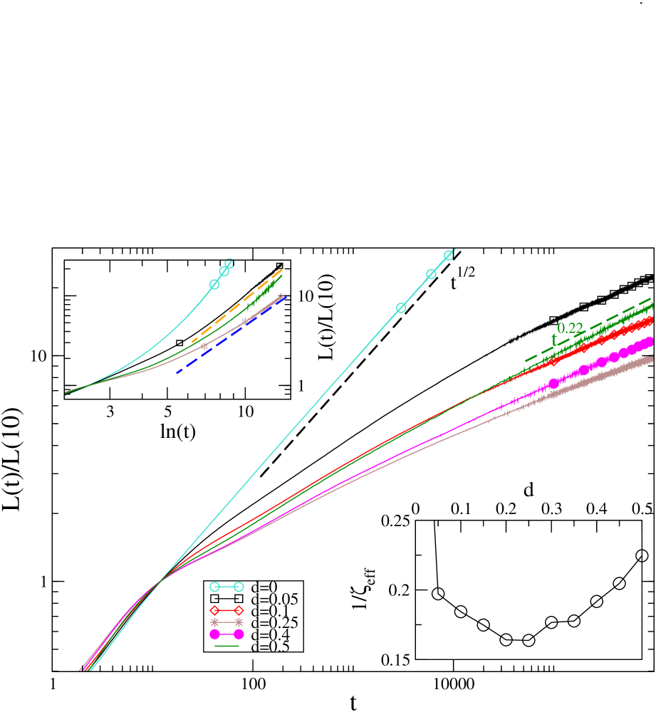
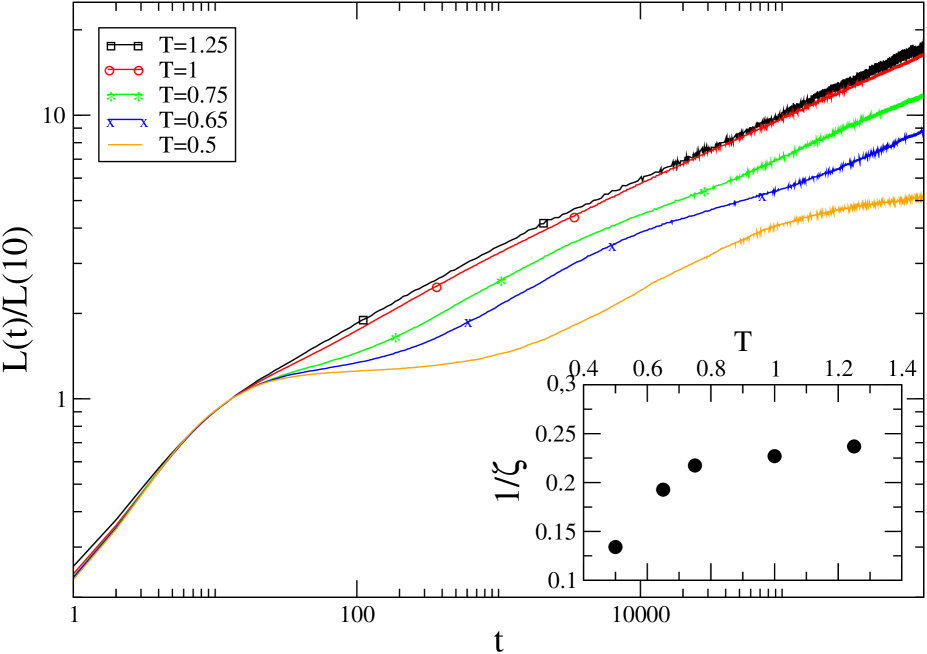
Figure 2: (Color online). Panel (a) (left) :$L(t)$ is plotted against $t$ in a double-log plot for a quench of the ARBIM to $T=\epsilon$, with $\epsilon=J_{0}$ and different values of $d$ specified in the key. The black-dashed line is the pure-case power-law $L(t)\propto t^{1/2}$ and the green-dashed one is the fit $L(t)\sim t^{0.22}$ at $d=d_{c}$. In the upper inset some of the curves of the main picture are plotted against $\ln t$ on a double-log plot. The orange-dashed and blue-dashed lines are the fits $y=0.03\cdot[\ln t]^{2.5}$ and $y=0.04\cdot[\ln t]^{2.1}$, respectively. In the inset the effective exponent $1/\zeta_{eff}$ is plotted against $d$. Panel (b) (right): $L(t)$ is plotted against $t$ in a double-log plot for a quench of the ARBIM to different final temperatures (specified in the key, curves lower upon decreasing temperature), with $\epsilon=J_{0}$ and $d=0.5$. In the inset the exponent $1/\zeta(\epsilon=J_{0},T,d=d_{c})$, obtained from a fit of the curves from $t=10^{2}$ onwards, is plotted against $T$.

III.2 $\epsilon<J_{0}$

Evidences supporting an interpretation in terms of the existence of three fixed points along the $\epsilon=J_{0}$ axis were discussed in the previous Section. Here we show that a similar structure is observed for any value of $\epsilon$. In order to do that we have scanned the parameter space by a set of cuts along lines with fixed $\epsilon$. An example (with $\epsilon=3/4\,J_{0}$) is shown in Fig. 1 with an horizontal dashed magenta line. The behavior of $L(t)$ along this line is reported in Fig. 3. Even if, when $\epsilon<J_{0}$, asymptotic coarsening occurs for any value of $d$ (the brown region in Fig. 1 is peculiar to the case with $\epsilon=J_{0}$) for sufficiently low temperatures, in order to compare the data to those for $\epsilon=J_{0}$ discussed in the previous Section III.1 (Fig. 2) let us initially restrict the discussion to the cases with $d\leq d_{c}=0.5$, which are shown in the left panel of the figure. For these values of $d$ we see a pattern qualitatively similar to that observed for $\epsilon=J_{0}$ (Fig. 2): Starting from the power-law $L(t)\sim t^{1/2}$ of the pure case $d=0$, the growth of $L(t)$ slows down up to a certain value $d^{*}(\epsilon)\simeq 0.3$ and then speeds up again reaching at $d=d_{c}=1/2$ a form compatible with a power-law $L(t)\sim t^{1/\zeta(\epsilon,T,d)}$ with an exponent $1/\zeta(\epsilon=3/4\,J_{0}/2,T=\epsilon,d)\simeq 0.2$ roughly similar to the one $1/\zeta(\epsilon=J_{0},T=\epsilon,d_{c})\simeq 0.22$ observed for $\epsilon=J_{0}$. The most notable difference with the case $\epsilon=J_{0}$ is the somewhat larger value of $d^{*}$, since we have here $d^{*}(\epsilon=3/4\,J_{0})\simeq 0.3>d^{*}(\epsilon=J_{0})\simeq 0.25$. The fact that $d^{*}$ is closer to $d_{c}$ than for $\epsilon=J_{0}$ makes the corresponding curves closer and the non-monotonic behavior less evident than in Fig. 2 (this can be better appreciated in the lower inset of the left part of Fig. 3, where a magnification the large-time portion of the figure is shown, or by inspection of the effective exponent $1/\zeta_{eff}$ reported in the inset of the right panel of the figure). In the upper set of Fig. (2) some of the curves displayed in the main picture are plotted against $\ln t$ on a double logarithmic scale since, as explained in Sec. III.1, this is a useful representation to check for a logarithmic growth-law. While the curves for $d=0$ and $d=d_{c}$ bend upward, signaling a growth faster than a logarithmic one, the one for $d=0.1$ can be interpreted, also in this case, as converging to a straight line. Fitting all the data in the last decade with the logarithmic form of Sec. III.1, one finds $1/\psi=2.4,2.3,2.1$ for $d=0.1,0.2,0.3$ respectively.

Clearly, although the overall behavior is similar, the interpretation of the cases with $\epsilon<J_{0}$ cannot follow literally the one for $\epsilon=J_{0}$, which was relying on the geometrical properties of a diluted system. However, this very same pattern of behaviors suggests that, since at low temperatures interfaces are located preferentially on the weak bonds $J_{ij}=J_{0}-\epsilon$, what really matters is the topology of the network of this set of bonds. At $d=d_{c}=1/2$ such network is a percolation fractal and this turns the logarithmic growth into a power-law one.

Let us now go back to the data with $d>d_{c}=1/2$ (still with $\epsilon=3/4J_{0}$) where, at variance with the case $\epsilon=J_{0}$ discussed in Sec. III.1, asymptotic phase-ordering may still occur. In this region one observes in the right panel of Fig. 3 that the curves bend upward as time elapses. Furthermore the growth-law becomes faster and faster as $d$ is raised from $d=d_{c}$ up to $d=1$. This can be interpreted as follows: Right at $d=1$ the system is a pure one with $J_{ij}\equiv J_{0}+\epsilon$ and the power-law $L(t)\sim t^{1/2}$ holds. This is analogous to the case with $d=0$, apart from a trivial shift of the value of the coupling constants. However, starting from this pure case with $d=1$, the effect of lowering $d$ is very different from the one occurring when, starting from the pure case $d=0$, $d$ is increased. In the former case by lowering $d$ one introduces strong bonds $J_{ij}=J_{0}+\epsilon$ in a majority background of week ones $J_{ij}=J_{0}-\epsilon$. Instead, in the second case, by increasing $d$ one does precisely the opposite, introducing strong bonds in a background of weak ones. Although these two situations might look symmetrical on purely geometrical grounds, they are not so from the energetic point of view. In fact a weak bond acts as an attractive pinning point for a wandering interface and an activation energy is required to leave it. This brings in the slow logarithmic growth-law for $0<d<d_{c}$. Conversely, for $d>d_{c}$ the strong bonds form finite repulsive regions which the interfaces manage to overcome without activation. Therefore, in the whole region with $d>d_{c}$ coarsening is expected to proceed over the compact network of weak bonds with the pure asymptotic growth-law $L(t)\propto t^{1/2}$.

Clearly, for $d$ larger than $d_{c}$ but sufficiently close to $d_{c}$, we expect a crossover phenomenon with a growth-law initially influenced by the presence of the nearby $W$ line. The pure-like growth-law should set in when the domains size $L(t)$ has grown larger than the typical size of the clusters of strong bonds $J_{ij}=J_{0}-\epsilon$. Hence the crossover to the late $L(t)\propto t^{1/2}$ behavior should occur earlier upon increasing $d$.

These expected behaviors are consistent with what we observe in Fig. 3. The data show a gradual crossover as $d$ is increased above $d_{c}$ which occurs earlier raising $d$. The upward bending of the curves shows that the effective exponent is bound to increase above the values measured in the time accessed in the simulations. For $d=0.9$ the growth-law is asymptotically very close to the pure one, as indicated by the effective exponent $1/\zeta_{eff}\lesssim 0.46$ (see inset) which grows up to $1/\zeta_{eff}\simeq 0.47$ if computed for $t>5\cdot 10^{5}$.

Repeating the simulations for different values of $\epsilon$, in the whole range $0<\epsilon\leq J_{0}$, we find a structure similar to the case $\epsilon=3/4J_{0}$ discussed insofar, with a value of $d^{*}$ which steadily increases as $\epsilon$ is lowered (specifically we find $d^{*}(\epsilon=J_{0}/2)\simeq 0.35$, $d^{*}(\epsilon=J_{0}/4)\simeq 0.4-0.45$)). This can be interpreted as a line of attractive fixed points, pictorially drawn dot-dashed in red in Fig. 1, which, starting from $S$ reaches the $d$ axis. Next to it, there is also a line of W-like points which starts from $W$ (depicted in green). Along this line the two kinds of bonds ($J_{ij}=J_{0}\pm\epsilon$) are arranged on a percolation network and $L(t)\sim t^{1/\zeta(\epsilon,T,d)}$, similarly to what occurs at W. Concerning the exponent $\zeta(\epsilon,T,d)$ we have found $1/\zeta\simeq 0.2$, roughly irrespectively of the value of $\epsilon$, suggesting that this exponent depends sensibly only on the ratio $\epsilon/T$. The power-law behavior observed at $d_{c}$ and the properties of the exponent $\zeta$ can be understood by considering what is observed on a simple model based on a deterministic fractal network, as we will discuss in Sec. IV.3.

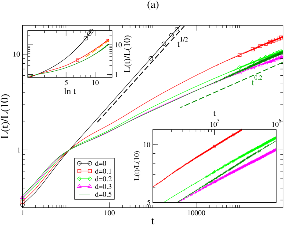
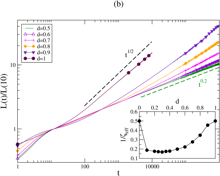
Figure 3: (Color online). $L(t)$ is plotted against $t$ in a double-log plot for a quench of the ARBIM to $T=\epsilon$, with $\epsilon=3/4\,J_{0}$ and different values of $d$ specified in the key. Panel (a) (left) shows the cases with $0\leq d\leq d_{c}$, the right one those with $d_{c}\leq d\leq 1$. The inset is a zoom on the curves in the last two decades. The black-dashed line is the pure-case power-law $L(t)\propto t^{1/2}$. The green-dashed line is the power-law $L(t)\propto t^{0.2}$. In the upper inset some of the curves of the main picture are plotted against $\ln t$ on a double-log plot. The orange-dashed line is the fit $y=0.03\cdot[\ln t]^{2.4}$. Panel (b) (right) shows the cases with $d_{c}\leq d\leq 1$. In the inset the behavior of the effective exponent $1/\zeta_{eff}$ is shown for the whole range of $0\leq d\leq 1$.

III.3 Summary of the results for the ARBIM

Let us briefly summarize the results for the ARBIM. First of all our results confirm the existence of a rich interplay between the behavior of the pure system and two other types of dynamical behaviors caused by the inhomogeneities, which are characterized respectively by logarithmic or by temperature-dependent power-law growth of $L(t)$. This can be interpreted along the lines of what has been previously found for the SDIM: Moving along the segment with $\epsilon=J_{0}$ (turquoise in Fig. 1) one encounters three fixed points, the pure one at $d=0$ and those denoted with the letters $S$ and $W$. $W$ is located at the percolation point $d_{c}=0.5$ and $S$ at a value $d^{*}(\epsilon=J_{0})\simeq 0.25$ roughly half-way between $d=0$ and $d=d_{c}$. At $W$ the topology of the substrate is such that the critical temperature of the Ising model defined on it is $T_{c}=0$ and this, according to the conjecture proposed in lastparma implies a power-law growth $L(t)\sim t^{1/\zeta}$. Since $W$ is a repulsive fixed point the dynamics is always ruled by the attractive point $S$ for any $0<d<d_{c}$, resulting in an asymptotic logarithmic growth. However the power-laws associated to the pure fixed point with $d=0$ or to $W$ may show up preasymptotically due to a crossover phenomenon.

We have found that this same pattern persists also for $\epsilon<J_{0}$. Hence, this means that $S$ and $W$ are not isolated fixed points, but that each of them belongs to two lines of fixed points extending from $\epsilon=J_{0}$ down to $\epsilon=0$. In particular, the $W$ line appears to be located at $d=0.5$, irrespective of $\epsilon$, and is characterized by the asymptotic power-law $L(t)\sim t^{1/\zeta}$. This means that in the low temperature limit what matters for power-law growth is that the network of the two kind of bonds are at the percolation point. An argument developed for a deterministic fractal structure supporting the existence of a power-law growth also for $\epsilon\neq J_{0}$ will be presented in Sec. IV. The location of $d^{*}$, on the other hand, is found to depend on $\epsilon$ and to approach $d_{c}$ as $\epsilon\to 0$, as pictorially shown in Fig. 1.

In agreement with the above structure, the growth-law has been found to display the following features:

• i) Quenches to a region where the system is pure (blue lines in Fig. 1): Pure power-law behavior $L(t)\propto t^{1/2}$ from an early microscopic time $t_{early}(\epsilon,T,d)$ onwards.

• ii) Quenches to the S-line (dot-dashed red in Fig. 1): Logarithmic behavior $L(t)\propto(\ln t)^{1/\psi}$ from the microscopic time $t_{early}(\epsilon,T,d)$ onwards.

• iii) Quenches to the W-line (continuous green in Fig. 1): Disordered power-law behavior $L(t)\propto t^{1/\zeta(\epsilon,T,d)}$ from $t_{early}(\epsilon,T,d)$ onwards. Our data suggest that $\zeta$ depends sensibly only on the ratio $\epsilon/T$.

• iv) Quenches to a point with disorder on the left of the S-line: A crossover from an early pure behavior $L(t)\propto t^{1/2}$ for $t_{early}(\epsilon,T,d)<t<t_{cross}(\epsilon,T,d)$ to logarithmic behavior for $t>t_{cross}(\epsilon,T,d)$ (with $t_{cross}(\epsilon,T,d)$ decreasing towards $t_{early}(\epsilon,T,d^{*}(\epsilon))$ upon approaching the S-line).

• v) Quenches between the S and the W-line: A crossover from an early disordered power-law behavior $L(t)\propto t^{1/\zeta(\epsilon,T,d)}$ for $t_{early}(\epsilon,T,d)<t<t_{cross}(\epsilon,T,d)$ to logarithmic behavior for $t>t_{cross}(\epsilon,T,d)$ (with $t_{cross}$ increasing upon approaching the $W$-line).

• vi) Quenches to a point with disorder on the right of the W-line (only for $\epsilon<J_{0}$): A crossover from an early disordered power-law behavior $L(t)\propto t^{1/\zeta(\epsilon,T,d)}$ for $t_{early}<t<t_{cross}(\epsilon,T,d)$ to the pure behavior $L(t)\propto t^{1/2}$ for $t>t_{cross}(\epsilon,T,d)$ (with $t_{cross}(\epsilon,T,d)$ decreasing towards $t_{cross}(\epsilon,T,d=1)$ moving away from the $W$-line).

We mention that the pattern of asymptotic behaviors summarized above is a low-temperature feature.

IV Deterministic fractal networks

In this section we study two deterministic fractal networks which can be considered as a simple paradigm explaining the ARBIM dynamical behavior. The structures that we will consider are generalizations of the Sierpinski gasket (SG) and of the Sierpinski carpet (SC). As we will discuss below, these networks can be considered representative of structures with a vanishing or with a finite critical temperature, respectively.

The SG is a network that can be built recursively as shown in Fig. 4 (upper panel). Starting from a primitive three-spin triangular object, the so called generation-one, the second generation is built by merging three generation-one structures, and the procedure is then repeated many times iteratively. As it can be seen in the lower panel of the figure the SG can be embedded on a triangular lattice. In this picture the bonds of the lattice belonging to the fractal network are plotted in black while the remaining ones, in the voids of the SG, are red. In this way the SG can be regarded as a triangular lattice with a deterministic bond dilution. Notice that the SG is a weak structure, in the sense previously discussed for the percolation network, because the removal of a finite number of links can serve to disconnect arbitrarily large parts of the structure (an example of such cutting bonds is shown in Fig. 4). For this reason the critical temperature of the Ising model on the SG is $T_{c}=0$.

The SC Gefen is a structure similar to the gasket, for which the recursive construction starts with a primitive four-spin square object, as shown in Fig. 4. Similarly to the SG it can be embedded in a two-dimensional regular lattice, although squared instead of triangular. The most important difference between the SC and the SG is that cutting bonds, which are present in the former, are absent in the latter. Related to that, the critical temperature of the Ising model defined on the SC is finite.

We now introduce a spin model on the embedding lattices of these structures (either triangular or squared) by defining Ising variables governed by the Hamiltonian (1). The coupling constants $J_{ij}$ take the value $J_{0}+\epsilon$ on the primary network (either the SG or the SC), and $J_{0}-\epsilon$ in the voids (namely the dashed-red bonds in Fig. 4) and similarly for the SC. Clearly, for $\epsilon\equiv 0$ one recovers the usual Ising model on the homogeneous (triangular or squared) lattice and $\epsilon=J_{0}$ corresponds to the Ising model defined on the original SG and SC fractal networks.

The dynamics is that described in Sec. II.2. The models introduced above will be denoted in the following as the generalized Sierpinski gasket (or carpet) Ising model (GSGIM or GSCIM).

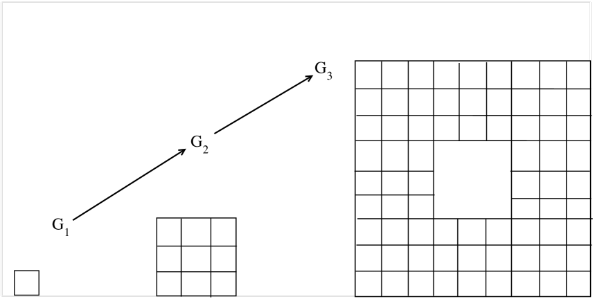
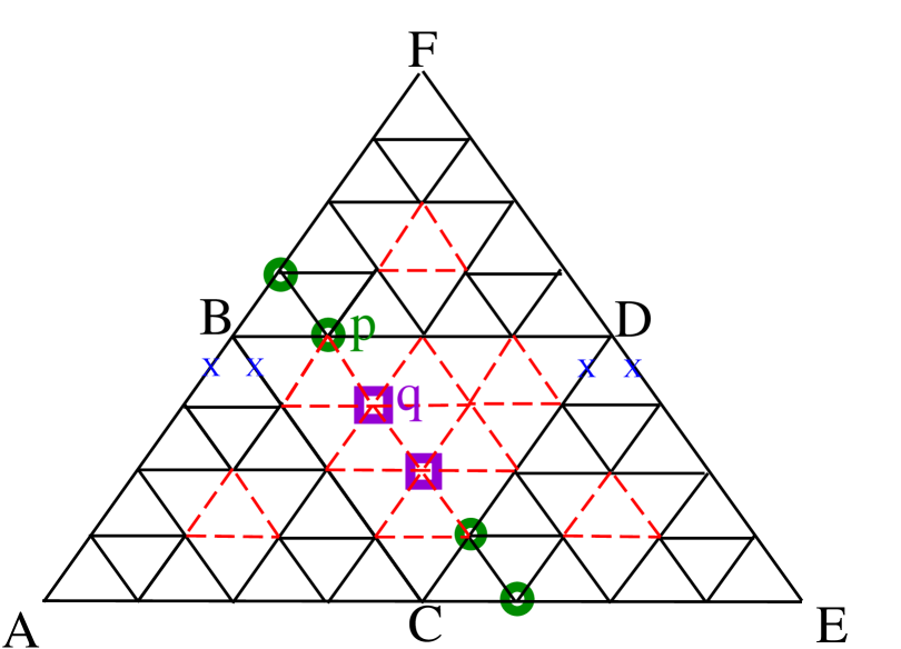
Figure 4: (Color online). Upper panels: Recursive construction of the SG and of the SC. Lower panel: The SG (in black) embedded in a triangular lattice (dashed-red). Bonds marked with a blue X are the cutting bonds.

IV.1 Simulation details

We have performed a series of numerical simulations of the deterministic fractal models described above by considering quenches to different final temperatures for a SG of $N=2100225$ sites, corresponding to a fractal network of the 11-th generation, and on a SC of $N=2125764$ sites, corresponding to a fractal of 7-th generation. Data are averaged over 2-500 independent runs. The other details of the simulations are as described in Sec. III for the ARBIM.

IV.2 $\epsilon\equiv J_{0}$

Let us start by recalling what is known for the phase-ordering of the Ising model with a coupling constant $J$ on the usual SG. Since this is a diluted structure with $T_{c}=0$ it can be considered to be comparable in some sense to the GSGIM with the choice $J_{0}=J/2,\epsilon=J_{0}$, namely at the point W. The Ising model on the SG was studied in Ref. parma ; lastparma where it was shown that $L(t)$ grows as a power-law with a temperature dependent exponent $L(t)\simeq t^{1/\zeta(T)}$. This has to be compared to what observed in the ARBIM at the fixed point W where, as shown in Sec. III.1, a similar power-law is observed. For low temperatures the algebraic behavior is decorated by a periodic oscillation which, as discussed in parma ; lastparma , is related to the recursive construction of the network. We notice, by the way, that similar oscillations are observed also in disordered models, such as the ARBIM considered above, at sufficiently low temperatures (lower than the ones used for simulations in this paper). In lastparma it was shown that the algebraic behavior can be understood in terms of the scaling of the barriers which tend to pin the displacement of interfaces. In the following we briefly sketch the argument (more details can be found in Ref. lastparma ).

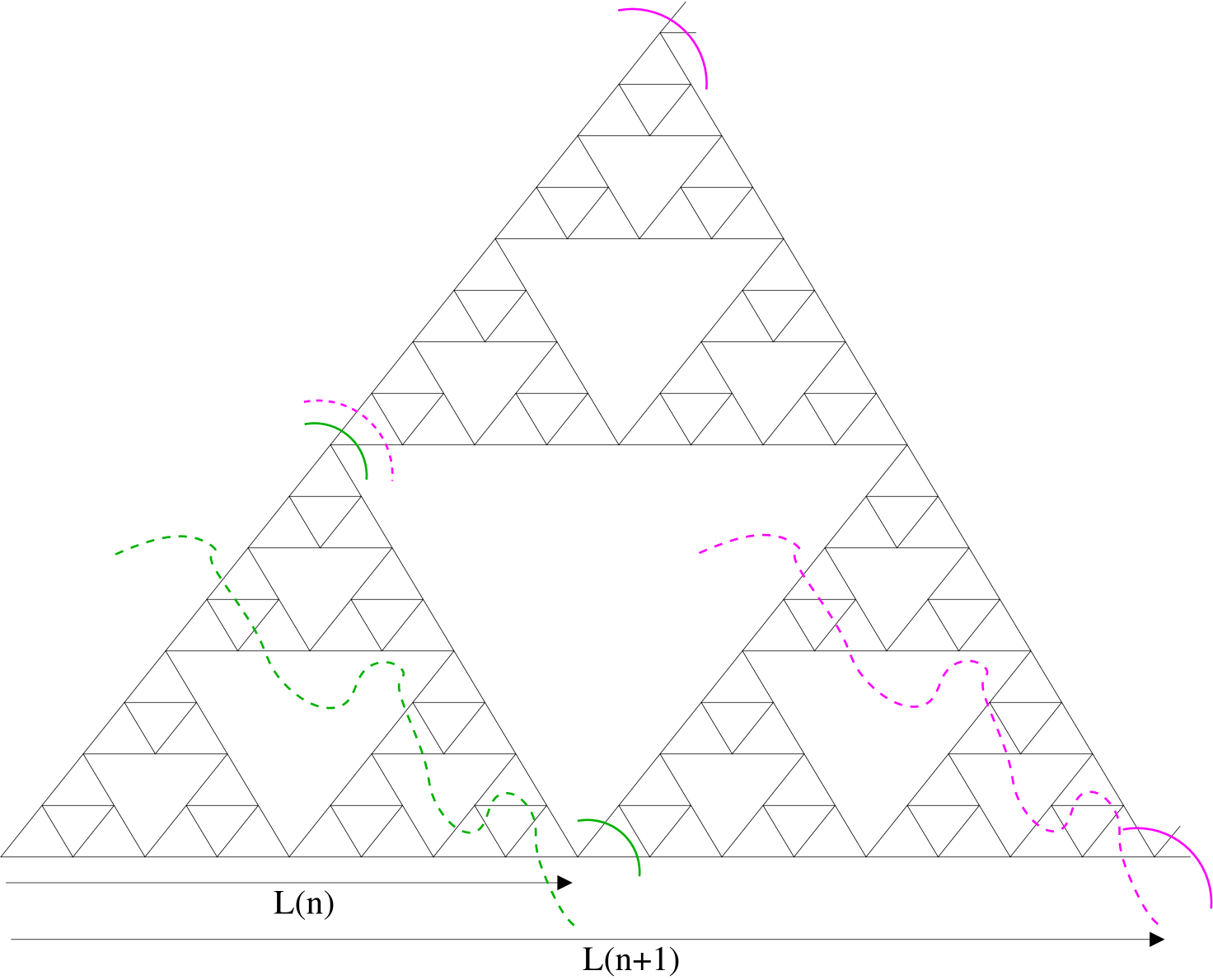
Figure 5: (Color online). Sketch of the movement of an interface on the SG.

Fig. 5 illustrates pictorially the evolution of an interface which progressively spans a part of the structure. Initially, the position of the domain wall is outside the figure, in the left corner. This means that all the spins are, say, down. As time goes on, the interface enters the graph by moving across the intermediate position $I_{n}^{(max)}$ indicated by a dotted green line (this means that spins on the left of the green line have been reversed up). The index $n$ refers to the fact that the interface is currently spanning the $n$-th generation of the fractal network. When the spins of the whole generation $n$ have been reversed, the interface, depicted with two green continuous arches in the middle of the sructure, is located in the configuration $I_{n}^{(min)}$ on the four cutting bonds. Since the energy of a domain wall is $2J$ times its length, it is clear that in $I_{n}^{(min)}$ the interface has a minimum energy $E_{n}^{(min)}=8J$ (notice that this quantity is independent of $n$). Let us assume that the highest energy $E_{n}^{(max)}$ of the system during the above process was reached in the (generic) configuration $I_{n}^{(max)}$, so that a barrier of height ${\cal E}_{n}=E_{n}^{(max)}-E_{n}^{(min)}$ has been crossed. Now the interface must proceed again to the right in order to reverse all the spins of the next generation $n+1$, thus reaching the position $I_{n+1}^{(min)}$ located on the other four cutting bonds, and indicated by the couple of continuous magenta arches on the upper and lower right corners of the structure (all the spins in the figure at this stage have then been reversed). Also this configuration has an energy equal to $E^{(min)}$. This configuration can be reached by sequentially reversing parts of generation $n$ of the structure (e.g. by first reversing another triangle of generation $n$, say the lower-right one in Fig. 5). This event is analogous to the one described before. In particular, the interface in the intermediate position $I_{n+1}^{(max)}$, depicted with a dashed-magenta line on the right of the structure, is analogous to the previous one at $I_{n}^{(max)}$ (dotted-green), except for the presence of an extra part which in the present example is indicated with a dashed-magenta arch in the middle of the left side. Denoting with $E_{n+1}^{(max)}$ the maximum energy reached by the system in the reversal of the $n+1$ generation, one concludes that $E_{n+1}^{(max)}=E_{n}^{(max)}+4J$, where $4J$ is the extra amount of energy due to the new part of interface (the dotted-magenta arch in the middle of the left side in the figure). Then ${\cal E}_{n+1}\simeq{\cal E}_{n}+4J$. Rewriting ${\cal E}$ in terms of the size $L_{n}\simeq 2^{n}-1$ of the $n$-th generation, using $L_{n+1}\simeq 2\cdot L_{n}$, one has ${\cal E}(2\cdot L_{n})\simeq{\cal E}(L_{n})+4J$. From this relation, dropping the index $n$, one has ${\cal E}\simeq\frac{4J}{\ln 2}\ln L$. Assuming an Arrhenius time $t\propto e^{\frac{{\cal E}}{K_{B}T}}$ to overcome the barrier, we arrive at a algebraic growth law $L(t)\sim t^{\frac{1}{\zeta(T)}}$ with

$$\zeta\simeq\frac{4}{k_{B}\ln 2}\,\frac{J}{T},$$ (6)

at low temperatures. The argument has been developed for the particular SG structure but it is expected to hold more generally for any finitely ramified deterministic fractal network and also for disordered structures with $T_{c}=0$, since the key ingredient is their weakness, namely the possibility to disconnect an arbitrary large part of the network by cutting a finite number of links. Due to that, the energy barriers that trap the interfaces on the cutting bonds grow as slow as a logarithm of the size of the domains.

A completely different situation is encountered when the Ising model is defined on the SC. In this case, due to the absence of cutting bonds, an argument similar to one presented above shows that the pinning energy of the interfaces grows faster - in an algebraic way - with the size of the ordered domains. Details can be found in lastparma .

IV.3 $0<\epsilon<J_{0}$

We have shown in Sec. III.2 that in the ARBIM the characteristic power-law behavior $L(t)\sim t^{1/\zeta}$ of the point W is observed not only at W but along the whole line with $d=1/2$, the only effect of changing $\epsilon$ is possibly to change the exponent $1/\zeta$. Our analogy suggests that the same behavior should be observed also in the GSGIM. We have performed a set of simulations with a small value of $J_{0}/\epsilon$ ($\epsilon/J_{0}=10^{-1}$) and another for a much larger value of this parameter ($\epsilon/J_{0}=0.9$). For each choice of $\epsilon$ we have considered different values of the quenching temperature $T$. The results of our simulations are shown in Fig. 6.

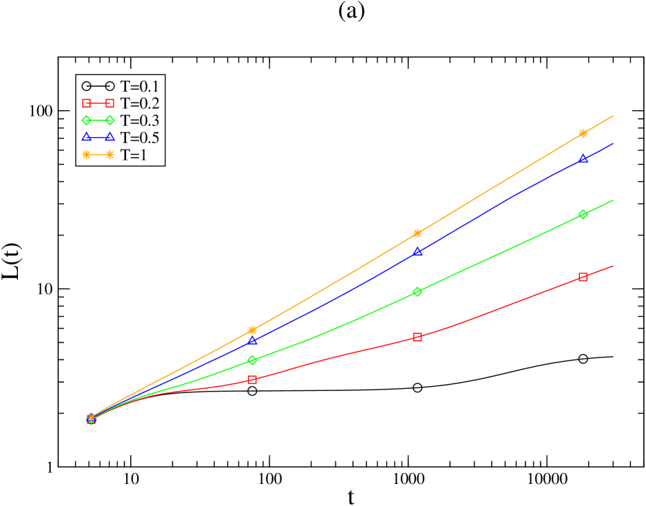
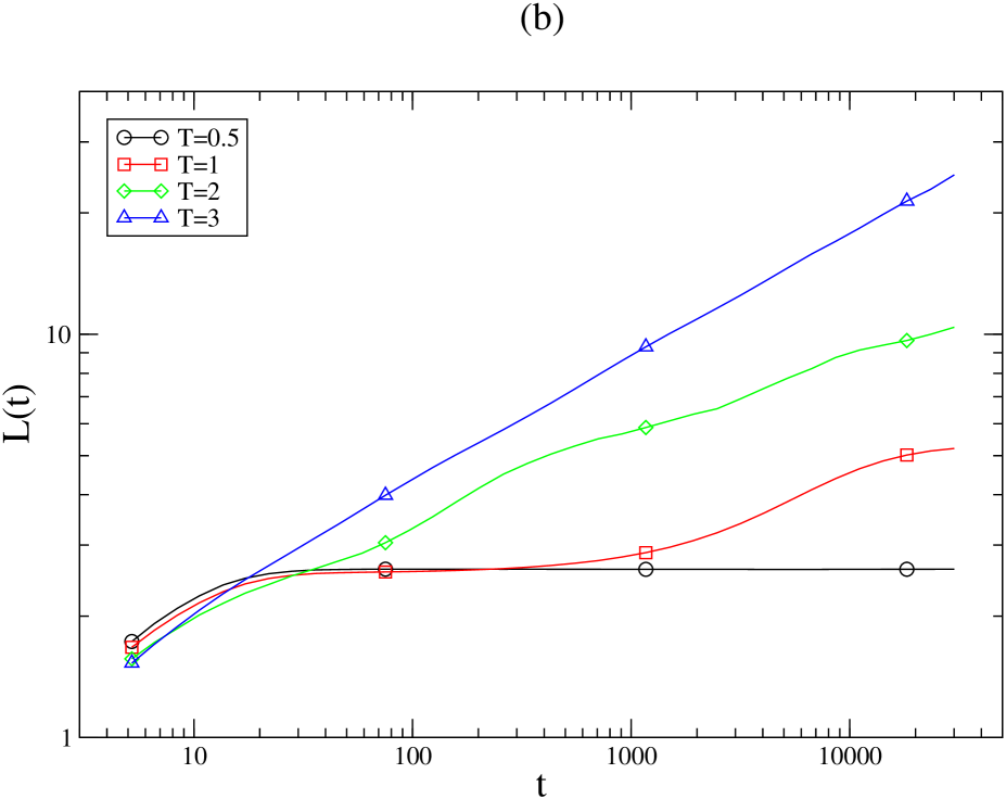
Figure 6: (Color online). $L(t)$ for the GSGIM with $\epsilon/J_{0}=10^{-1}$ (panel (a), left) and $\epsilon/J_{0}=0.9$ (panel (b), right).

Starting with the case with $\epsilon/J_{0}=10^{-1}$ (left panel of Fig. 6) we see that, as expected, the growth of $L(t)$ is similar to the one observed in the Ising model on the SG (namely the case with $\epsilon/J_{0}=1$), namely a power-law decorated by periodic oscillations whose amplitude increases upon lowering $T/\epsilon$. This behavior is also analogous to what observed in the ARBIM for $d=1/2$ (except for the oscillations), where the network of bonds with $J_{ij}=J_{0}+\epsilon$ is a percolation fractal for which the Ising critical temperature vanishes as in the SG.

For $\epsilon/J_{0}=0.9$ the situation is qualitatively similar, with the quantitative difference of a much slower growth, for a given temperature, with respect to the case with for $\epsilon/J_{0}=0.1$. This is expected since the height of barriers is related to $\epsilon$. However, comparing curves for $\epsilon/J_{0}=0.9$ and $\epsilon/J_{0}=10^{-1}$ with a similar value of $\epsilon/T$, one finds roughly similar exponents (for instance for $\epsilon/J_{0}=0.1,T=0.2$ and $\epsilon/J_{0}=0.9,T=2$ one has $1/\zeta\simeq 0.23$ and $1/\zeta\simeq 0.21$ respectively, and for $\epsilon/J_{0}=0.1,T=0.3$ and $\epsilon/J_{0}=0.9,T=3$ one has $1/\zeta\simeq 0.34$ and $1/\zeta\simeq 0.31$ respectively). This shows that the growth-law depends at most weakly on the parameter $\epsilon/T$.

In order to understand the origin of these behaviors we go back to the argument of Sec. IV.2 for the Ising model on the SG. When the interface is in the configuration $I_{n}^{(min)}$ sketched with two continuous-green arches in the middle of the structure in Fig. 5, the lower-left triangle ABC of Fig. 4 contains up spins and the rest of the structure is down (and there are no spins in the voids). The next spin to be reversed is one of those marked with a bold-green circle. Since these are equivalent, to be concrete let us chose it to be the one denoted by the letter p. The energy needed to flip it is easily computed to be

$${\cal E}_{p}=4J$$ (7)

In the case of the GSGIM the dynamics proceeds along the same lines. However, starting again with the interface in the configuration with two continuous-green arches, besides the spin marked with the green circle in Fig. 4 also those indicated by a heavy violet box can flip. Computing the energetic barriers one can easily convince that one of the latter is the next spin to be reversed (for which the energy barrier is lower). Let us stipulate this to be the one denoted with the letter q. The energy cost turns out to be $4(J_{0}-\epsilon)$. After reversing q, spin p will be flipped, which requires an energy $8\epsilon$. The maximum energy required to arrive to flip p is then

$${\cal E}_{p}^{GSGIM}=\max[4(J_{0}-\epsilon),8\epsilon]$$ (8)

At this point we are left back to the situation reached by the Ising model on the SG described before, since the blocked spin p has been flipped, and we can repeat the argument developed before to arrive to the conclusion that also in this case barriers grow logarithmically with the size of the domains, which in turn implies a temperature-dependent power-law growth of $L(t)$. Notice however that in the case of the GSGIM the reversal of p has been facilitated by the intermediate flipping of q. This, as we will show below, lowers the energy of the pinning barriers (still maintaining the logarithmic scaling with $L(t)$). In order to show this we must compare the energy scale to flip p in the GSGIM Eq. (8) to the one (7) of the Ising model on the SG with a coupling constant $J=(J_{0}+\epsilon)$ (namely, the one obtained from the GSGIM by removing altogether the bonds in the voids of the SG). The latter turns out to be always higher for $\epsilon<J_{0}$. Then, we can conclude that the evolution is faster in the GSGIM or, in other words, that the addition of the extra dashed-red bonds of Fig. 4 speeds up the dynamics. Indeed, for instance, extracting the effective exponent for the case with $\epsilon/J_{0}=10^{-1},T=1$ we find $1/\zeta\simeq 0.46$, a much larger value than that found for the Ising model on the SG with $J=J_{0}+\epsilon=1.1$ at the same temperature which is $1/\zeta\simeq 0.23$.

In order check the consistency of our conjectures we have performed a series of simulation analogous to those for the GSGIM also for the GSCIM. In this case, since on the SC cutting bonds are absent and the Ising model defined on it has $T_{c}>0$, we expect to see a situation similar to that observed in the ARBIM away from the line of fixed points W, namely an asymptotic logarithmic law for the domains size. For the Ising model defined on the SC, in fact, it was shown in lastparma that this is indeed the case. For the GSCIM the results for $L(t)$ are presented in Fig. 7. From the inset of this figure one sees that on a double log plot the data clearly bend downwards for both the values of $\epsilon/J_{0}$ considered. This indicates that the growth of the domains size is lower than a power-law. In the main figure the same data for $L(t)$ are plotted against $\ln t$, still in a double logarithmic scale. For a growth like $L\sim(\ln t)^{\phi}$ in this kind of plot one should observe a straight line with slope $\phi$. Due to the oscillating character of the data one cannot rich a clearcut evidence on the real form of $L(t)$. However, particularly for the higher values of temperatures considered, one can conclude that at least a logarithmic behavior describes much better the data with respect to a power-law. Notice that, also in this case, curves with comparable values of $\epsilon/T$ behave quite similarly, suggesting that this combination of parameters only weekly affects the dynamics.

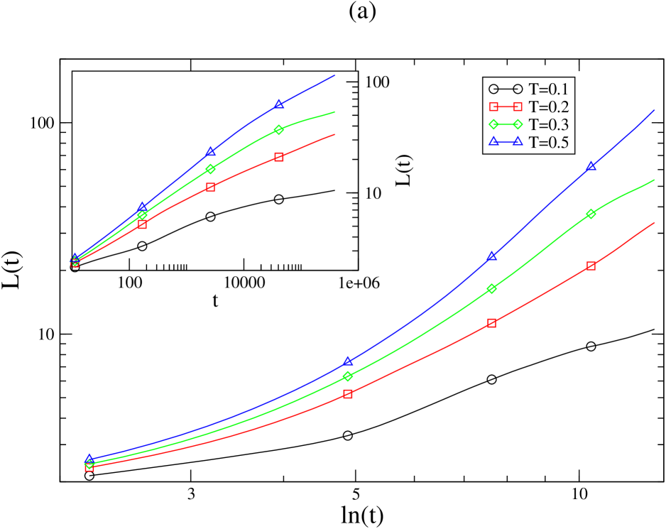
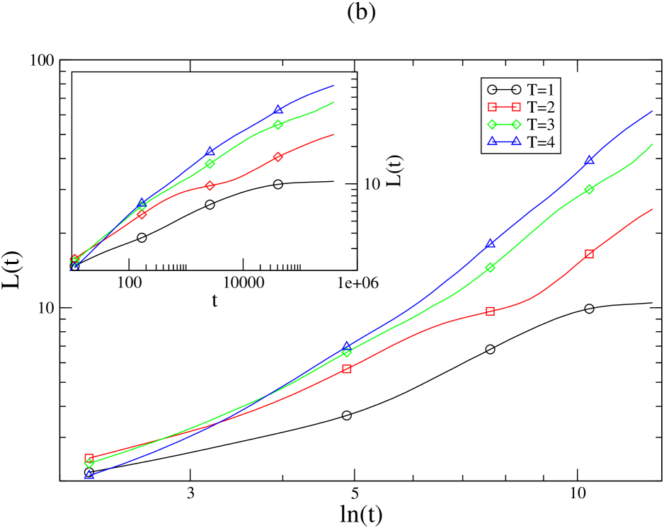
Figure 7: (Color online). $L(t)$ for the GSCIM with $\epsilon/J_{0}=10^{-1}$ (panel (a), left) and $\epsilon/J_{0}=0.9$ (panel (b), right).

IV.4 Summary of the results for the GSGIM and analogies with the ARBIM

In summary, we have shown the following analogies between the ARBIM and the paradigmatic models based on deterministic fractal networks:

• i) For $\epsilon=J_{0}$, when the randomness of the coupling constant amounts to bond dilution, one finds a power-law growth of the ordered domains (possibly with periodic oscillations) in those cases with weak diluted networks. This means the ARBIM at the percolation threshold or the GSGIM (since the SG has $T_{c}=0$).

• ii) One finds power-law growth also for $\epsilon<J_{0}$ in those cases where the network of the stronger bonds $J_{ij}=J_{0}+\epsilon$ is weak, i.e. in the ARBIM on the green W line schematized in Fig. 1, or in the GSGIM.

• iii) The growth-law slower than a power-law (of a logarithmic type) in all the other cases, namely when the network of bonds with $J_{ij}=J_{0}+\epsilon$ is not weak. This corresponds to the region of parameter space of the ARBIM away from the green W-line of Fig. 1 or, considering the fractal structures, in the GSCIM for any choice of the parameters.

These observations can be rationalized as follows: The GSGIM depends on the quantities $\epsilon/J_{0}$, $T/J_{0}$, whereas in the ARBIM the extra parameter $d$ is also present. The network of bonds $J_{ij}=J_{0}-\epsilon$ of the GSGIM, being a SG, is always weak. The dynamics of this model can then be understood considering that, in a sense, changing $\epsilon$ corresponds to drive the ARBIM along the green W-line. On the other hand, the GSCIM, which is based on a structure with no cutting bonds, corresponds to the ARBIM away from the line of fixed points W.

V Conclusions and perspectives

This paper was devoted to the study of phase-ordering on inhomogeneous systems, focusing on the growth-law of the ordered domains. Previous studies on systems with site dilution, either random diluted or deterministic lastparma , suggest that the growth-law is strongly affected by the topological properties of the substrate, namely the network of non-diluted sites, similarly to what is known for equilibrium properties. Specifically, it was shown that the growth-law is of a logarithmic type if the substrate is such that a finite-temperature phase-transition is present, whereas it turns to a to power-law on networks that do not support such phase-transition. This suggests that a similar correspondence could be at work also in systems whith different kinds of inhomogeneities.

In this paper we have studied this possibility by considering, as a first step, a system with bond dilution, a source of inhomogeneity different, but as close as possible, to that of site-diluted systems. Besides addressing the problem of the influence of topology on the non-equilibrium processes, our study is also ment to possibly shed some light on the nature of the power-law like pre-asymptotic regime in ferromagnetic systems with a random bond distribution CLMPZ ; various2 . In this perspective, we have undertaken a thorough investigation of the non-equilibrium evolution of a quenched random-bond Ising model, the ARBIM, where two kind of bonds with strength $J_{ij}=J_{0}\pm\epsilon$ occurring with relative probabilities $d$, $1-d$, are randomly seeded on a two-dimensional square-lattice. This allows us not only to study the case of bond dilution, corresponding to $\epsilon=J_{0}$, but also the generic case which, as discussed above, is relevant to the physics of disordered ferromagnets.

Our study shows that the whole pattern of behaviors of the model as its parameters (such as $\epsilon$, the quench temperature, and $d$) are varied can be interpreted in terms either of logarithmic or power-law growth laws, and of crossover phenomena between them, similarly to what was found in models with site dilution diluted . For $\epsilon=J_{0}$, when the randomness of the bonds amounts to a dilution, this interplay can be interpreted in terms of the topology of the substrate. Interestingly, this very interpretation provides a framework to the behavior of the system also for $\epsilon\neq J_{0}$, where the form of bond randomness does not amount to simple dilution.

To check the generality of such an interpretation, and in order to study the phenomenon on simpler systems, we have also considered a ferromagnetic model defined on deterministic substrates, such as the Sierpinski carpet and gasket, which do (or do not, respectively) support a finite-temperature phase-transition. According to the general conjecture put forth in lastparma , these models should represent two paradigmatic examples of logarithmic and power-law growth, because these behaviors are not expected to depend on specific details of the system, but they only rely on the presence of a critical point. Since these structures have the advantage to be deterministic, they can be regarded as toy systems where the properties observed in the more complex disordered cases, as in the ARBIM model, can be more carefully studied, checked and, possibly, understood. Indeed, by defining an Ising model with the same bimodal distribution of bonds as in the ARBIM, we were able to identify a similar pattern of behaviors to the one observed in the ARBIM.

Since the occurrence of preasymptotic power-laws followed by a logarithmic growth is observed also in systems with different kinds of quenched disorder as, for instance, random fields, it would be interesting to understand if a similar interpretation applies also in these cases. This would promote the conjecture put forth in this paper to a more general character.

Next to the behavior of $L(t)$, the role of disorder (and more generally of any source of inhomogeneity) is relevant for the form of the scaling functions of correlation and response functions altric . In particular the so-called superuniversality  10noirf , namely the property according to which $L(t)$ should depend on the strength of the disorder while the scaling functions should not, after some initial confirmations super1 ; super2 ; super3 ; super has been recently questioned diluted ; decandia ; CLMPZ ; variousnoi2 . In this respect, the results of this paper and their interpretation in terms of competition between different scaling behaviors strengthen previous findings against superuniversality.

Acknowledgments F.Corberi acknowledges financial support by MURST PRIN 2010HXAW77_005. E.Lippiello acknowledges financial support from the National Science Foundation under Grant No. NSF PHY11-25915.

References

- (1) A.J. Bray, Adv. Phys. 43, 357 (1994).
- (2) S. Puri, in Kinetics of Phase Transitions, edited by S. Puri and V. Wadhawan, CRC Press, Boca Raton (2009), p. 1.
- (3) M.Zannetti, in Kinetics of Phase Transitions (Ref. 2dinoirf ), p.153.
- (4) J.P.Bouchaud, L.F.Cugliandolo, J.Kurchan and M.Mezard, in Spin Glasses and Random Fields, edited by A.P.Young (World Scientific, Singapore, 1997).
- (5) F. Corberi, L. F. Cugliandolo, and H. Yoshino, in Dynamical Heterogeneities in Glasses, Colloids, and Granular Media, edited by L. Berthier, G. Biroli, J.-P. Bouchaud, L. Cipelletti, and W. Van Saarloos (Oxford University Press, Oxford, 2011).
- (6) F. Corberi, E. Lippiello, A. Mukherjee, S. Puri, M. Zannetti, Phys. Rev. E 88, 042129 (2013).
- (7) A. Sicilia, J. J. Arenzon, A. J. Bray and L. F. Cugliandolo, Europhys. Lett. 82, 1001 (2008); M. P. O. Loureiro, J. J. Arenzon, L. F. Cugliandolo, and A. Sicilia, Phys. Rev. E 81, 021129 (2010).
- (8) R. Paul, S. Puri and H. Rieger, Phys. Rev. E 71, 061109 (2005); R. Paul, G. Schehr and H. Rieger, Phys. Rev. E 75, 030104(R) (2007).
- (9) R. Paul, S. Puri and H. Rieger, Europhys. Lett. 68, 881 (2004).
- (10) M. Henkel and M. Pleimling, Europhys. Lett. 76, 561 (2006); Phys. Rev. B 78, 224419 (2008).
- (11) R. Burioni, F. Corberi, and A. Vezzani, Phys. Rev. E 87, 032160 (2013).
- (12) S. Puri, D. Chowdhury and N. Parekh, J. Phys. A 24, L1087 (1991).
- (13) F. Corberi, A. de Candia, E. Lippiello and M. Zannetti, Physica A 314, 454 (2002).
- (14) E. Lippiello, A. Mukherjee, S. Puri and M. Zannetti, Europhys. Lett. 90, 46006 (2010).
- (15) F. Corberi, E. Lippiello, A. Mukherjee, S. Puri and M. Zannetti, J. Stat. Mech.: Theory and Experiment P03016 (2011).
- (16) F. Corberi, E. Lippiello, A. Mukherjee, S. Puri, and M. Zannetti, Phys. Rev. E 85, 021141 (2012).
- (17) S. Puri and N. Parekh, J. Phys. A 26, 2777 (1993); E. Oguz, A. Chakrabarti, R. Toral and J.D. Gunton, Phys. Rev. B 42, 704 (1990); E. Oguz, J. Phys. A 27, 2985 (1994); C. Castellano, F. Corberi, U. Marini Bettolo Marconi, and A. Petri, J. Phys. IV France 08, Pr6-93 (1998).
- (18) M. Rao and A. Chakrabarti, Phys. Rev. Lett. 71, 3501 (1993); C. Aron, C. Chamon, L.F. Cugliandolo and M. Picco, J. Stat. Mech. P05016 (2008).
- (19) L.F. Cugliandolo, Physica A 389, 4360 (2010).
- (20) H. Park and M. Pleimling, Phys. Rev. B 82, 144406 (2010).
- (21) D.A. Huse and C.L. Henley, Phys. Rev. Lett. 54, 2708 (1985).
- (22) R. Burioni, F. Corberi, and A. Vezzani, J. Stat. Mech. (2010) P12024; J. Stat. Mech. (2009) P02040; R. Burioni, D. Cassi, F. Corberi, and A. Vezzani, Phys. Rev. E 75, 011113 (2007); Phys. Rev. Lett. 96, 235701 (2006).
- (23) D. Stauffer, Phys. Repts. 54, 1 (1979); D. Stauffer and A. Aharony, Introduction to Percolation Theory, Taylor and Francis, London 1994 (revised second edition).
- (24) F. Corberi, E. Lippiello, and M. Zannetti, Phys. Rev. E 63, 061506 (2001); Eur. Phys. J. B 24 (2001), 359; Phys.Rev. E 68, 046131 (2003); Phys.Rev. E 78, 011109 (2008); E. Lippiello, F. Corberi, A. Sarracino, and M. Zannetti, Phys. Rev. E 78, 041120 (2008); F. Corberi, and L.F. Cugliandolo, J. Stat. Mech. P05010 (2009).
- (25) F. Corberi, E. Lippiello, and M. Zannetti, Eur. Phys. J. B 24, 359 (2001).
- (26) F. Corberi, C. Castellano, E. Lippiello, and M. Zannetti, Phys. Rev. E 65, 066114 (2002); N. Andrenacci, F. Corberi, and E. Lippiello, Phys. Rev. E 74, 031111 (2006); E. Lippiello, F. Corberi, and M. Zannetti, Phys. Rev. E 71, 036104 (2005); R. Burioni, F.Corberi, and A. Vezzani, Phys. Rev. E 79, 041119 (2009); S. J. Cornell, K. Kaski, and R. B. Stinchcombe, Phys. Rev. B 44, 12263 (1991).
- (27) Y. Gefen, A. Aharony, Y. Shapir, and B. B. Mandelbrot, J. Phys. A 16, 435 (1983); Y. Gefen, A. Aharonyt, Y. Shapir, and B. B. Mandelbrot, J. Phys. A 17, 1277 (1984).
- (28) F. Corberi, E. Lippiello, and M. Zannetti, J. Stat. Mech. P07002 (2007). F. Corberi, C. Castellano, E. Lippiello, and M. Zannetti, Phys. Rev. E 70 017103 (2004).
- (29) A. Sicilia, J. J. Arenzon, A. J. Bray and L. F. Cugliandolo, Europhys. Lett. 82, 1001 (2008).