Non ambiguous structures on $\displaystyle 3$-manifolds and quantum symmetry defects

Abstract.

The state sums defining the quantum hyperbolic invariants (QHI) of hyperbolic oriented cusped $\displaystyle 3$-manifolds can be split in a “symmetrization” factor and a “reduced” state sum. We show that these factors are invariants on their own, that we call “symmetry defects” and “reduced QHI”, provided the manifolds are endowed with an additional “non ambiguous structure”, a new type of combinatorial structure that we introduce in this paper. A suitably normalized version of the symmetry defects applies to compact $\displaystyle 3$-manifolds endowed with $\displaystyle PSL_{2}(\mathbb{C})$-characters, beyond the case of cusped manifolds. Given a manifold $\displaystyle M$ with non empty boundary, we provide a partial “holographic” description of the non-ambiguous structures in terms of the intrinsic geometric topology of $\displaystyle\partial M$. Special instances of non ambiguous structures can be defined by means of taut triangulations, and the symmetry defects have a particularly nice behaviour on such “taut structures”. Natural examples of taut structures are carried by any mapping torus with punctured fibre of negative Euler characteristic, or by sutured manifold hierarchies. For a cusped hyperbolic $\displaystyle 3$-manifold $\displaystyle M$ which fibres over $\displaystyle S^{1}$, we address the question of determining whether the fibrations over a same fibered face of the Thurston ball define the same taut structure. We describe a few examples in detail. In particular, they show that the symmetry defects or the reduced QHI can distinguish taut structures associated to different fibrations of $\displaystyle M$. To support the guess that all this is an instance of a general behaviour of state sum invariants of $\displaystyle 3$-manifolds based on some theory of $\displaystyle 6j$-symbols, finally we describe similar results about reduced Turaev-Viro invariants.

¹ Institut Montpelliérain Alexander Grothendieck, Université de Montpellier, Case Courrier 51, 34095 Montpellier Cedex 5, France (sbaseilh@univ-montp2.fr)

² Dipartimento di Matematica, Università di Pisa, Largo Bruno Pontecorvo 5, 56127 Pisa, Italy (benedett@dm.unipi.it)

Keywords: $\displaystyle 3$-manifolds, taut triangulations, state sums, quantum invariants.

AMS subject classification: 57M27,57M50

1. Introduction

A first aim of this paper is to produce refinements of the quantum hyperbolic invariants (QHI) of hyperbolic cusped $\displaystyle 3$-manifolds (defined in [8], extending [5, 6]). But our thesis is that such refinements are instances of a sort of “universal” phenomenon concerning the quantum invariants of $\displaystyle 3$-manifolds based on some theory of $\displaystyle 6j$-symbols and defined by means of state sums over triangulations. At least this holds for every example to our knowledge (for instance the family of generalized Turaev-Viro invariants based on the $\displaystyle 6j$-symbols of any unimodular category, constructed in [32]). The arguments of these new invariants, that we call reduced invariants, are the same as those of the “unreduced” ones, but they apply to $\displaystyle 3$-manifolds equipped with an additional non ambiguous structure, a new type of combinatorial structure on compact oriented $\displaystyle 3$-manifolds that we introduce and investigate, pointing out in particular a strong relationship with the theory of taut triangulations.

Let us describe qualitatively this phenomenon.

$\displaystyle\bullet$ There is a “background theory”, usually given by a category of finite dimensional representations of a Hopf algebra; the “$\displaystyle 6j$-symbols” of the theory can be organized at first to produce a kind of “basic tensor”, that is, linear isomorphisms

$${\mathcal{B}}:V_{3}\otimes V_{1}\to V_{2}\otimes V_{0}$$

carried by an oriented $\displaystyle 3$-simplex equipped with a further “decoration”, say $\displaystyle d$, dictated by the background theory. Usually the $\displaystyle V_{j}$ are complex vector spaces of the same dimension. A $\displaystyle 3$-simplex is a tetrahedron $\displaystyle\Delta$ with ordered vertices $\displaystyle v_{0},v_{1},v_{2},v_{3}$; this can be encoded by a system $\displaystyle b$ of edge orientations (called a (local) branching) such that there are $\displaystyle j$-incoming edges at the vertex $\displaystyle v_{j}$. The $\displaystyle 2$-faces $\displaystyle F_{j}$ of $\displaystyle(\Delta,b)$ are ordered accordingly with the opposite vertices $\displaystyle v_{j}$, and we associate to the face $\displaystyle F_{j}$ the space $\displaystyle V_{j}$. This is the basic use of the branching to associate the tensor $\displaystyle{\mathcal{B}}={\mathcal{B}}(\Delta,b,d)$ to $\displaystyle(\Delta,b)$. But depending on the background theory, there are further subtler uses concerning the decoration $\displaystyle d$. For example, in quantum hyperbolic theory an ingredient of the decoration is a triple of shape parameters, which are scalars in $\displaystyle\mathbb{C}\setminus\{0,1\}$, associated to the triple of couples of opposite edges. These naturally occur with a cyclic ordering depending on the orientation of $\displaystyle\Delta$. The branching $\displaystyle b$ is used to select one linear ordering compatible with the cyclic one.

$\displaystyle\bullet$ Given a triangulation $\displaystyle T$ of some compact oriented $\displaystyle 3$-manifold $\displaystyle M$, we give each oriented tetrahedron $\displaystyle\Delta$ of $\displaystyle T$ a branching and a decoration, so that the system formed by such local data verifies certain global constraints (also dictated by the background theory). For example, for what concerns the local branchings we could require that the edge orientations of the tetrahedra match under the $\displaystyle 2$-face pairings in $\displaystyle T$, to produce a global branching $\displaystyle b$ of $\displaystyle T$. This is equivalent to promote $\displaystyle T$ to be a $\displaystyle\Delta$-complex (a generalized simplicial complex), a kind of object familiar in algebraic topology (see [21]). But it turns out that this is too demanding. On another hand, every oriented $\displaystyle 3$-simplex $\displaystyle(\Delta,b)$ carries a weaker structure, that is, a system of transverse co-orientations of its $\displaystyle 2$-faces such that two co-orientations are incoming and two are outgoing. We call it the local pre-branching $\displaystyle(\Delta,\omega_{b})$ induced by the branching $\displaystyle b$. We say that a system $\displaystyle\tilde{b}$ of local branchings of the tetrahedra of $\displaystyle T$ is a weak branching if their $\displaystyle 2$-face co-orientations match under the $\displaystyle 2$-face pairings, and we call such a system $\displaystyle\omega_{\tilde{b}}$ of co-orientations a global pre-branching of $\displaystyle T$. Pre-branchings occur, for instance, in the definition of taut triangulations [26]. But one eventually realizes that the notion of pre-branching is also the most fundamental global enhancement of $\displaystyle 3$-manifold triangulations in order to deal with “quantum state sums” (for any background theory). Given a weakly branched triangulation $\displaystyle(T,\tilde{b})$ endowed with a global decoration, say $\displaystyle{\mathcal{D}}$, we get a tensor network by associating the above basic tensor $\displaystyle{\mathcal{B}}(\Delta,b,d)$ to every decorated $\displaystyle 3$-simplex $\displaystyle(\Delta,b,d)$ of $\displaystyle(T,\tilde{b},{\mathcal{D}})$. The state sum $\displaystyle{\mathcal{B}}(T,\tilde{b},{\mathcal{D}})$ is by definition the total contraction of this network. We call it a reduced (or basic) state sum of the theory.

$\displaystyle\bullet$ In order to obtain invariants of the $\displaystyle 3$-manifold $\displaystyle M$ (possibly equipped with additional structures, as it happens in quantum hyperbolic theory) by means of such state sums, we have to mod out the arbitrary choices we have made, in particular the choice of the weak branching $\displaystyle\tilde{b}$. This gives rise to a more or less delicate procedure of symmetrization of the basic tensors, producing tensors of the same type, say $\displaystyle{\mathcal{S}}(\Delta,b,d)$, such that the corresponding state sums (ie. network total contraction) $\displaystyle{\mathcal{S}}(T,\tilde{b},{\mathcal{D}})$ have the required invariance properties.

$\displaystyle\bullet$ One might wonder anyway whether the reduced state sums $\displaystyle{\mathcal{B}}(T,\tilde{b},{\mathcal{D}})$ define some kind of $\displaystyle 3$-dimensional invariant. For example it holds that, keeping the decoration $\displaystyle{\mathcal{D}}$ fixed, the value of $\displaystyle{\mathcal{B}}(T,\tilde{b},{\mathcal{D}})$ depends only on the underlying pre-branching $\displaystyle\omega_{\tilde{b}}$, not on $\displaystyle\tilde{b}$ itself. Moreover, the state sums verify a highly non trivial system of functional identities which apparently is formally the same for every background theory; this system corresponds to a restricted system of “moves” on pre-branched triangulations, called non ambiguous transits. Then the notion of non ambiguous structure on $\displaystyle M$ arises as an equivalence class of pre-branched triangulations of $\displaystyle M$ up to non ambiguous transits.

In order to substantiate our thesis, in the present paper we spell out the case of the quantum hyperbolic state sums, and in the Appendix, the most fundamental prototype of this business, the Turaev-Viro state sums [31].

Having in mind this strong motivation (at least in our opinion), the theory of non ambiguous structures can be introduced and developed by itself, without any reference to any specific $\displaystyle 6j$-symbols theory. It is remarkable nevertheless that in doing it, some issues of the quantum hyperbolic machinery emerge. We will develop two instances of non ambiguous structures; the most important is based on ideal triangulations of $\displaystyle 3$-manifolds that are the interior of compact connected oriented $\displaystyle 3$-manifolds $\displaystyle M$ with non empty boundary (Sections 2 to 6); the other is based on relative “distinguished triangulations” $\displaystyle(T,H)$ of $\displaystyle(M,L)$, where $\displaystyle M$ is a compact closed oriented $\displaystyle 3$-manifold and $\displaystyle L$ is a non empty link in $\displaystyle M$ (Section 7).

In the rest of this introduction we describe more features of the non ambiguous structures (Sections 1.1 and 1.2) and our results about reduced quantum hyperbolic invariants (Section 1.3).

1.1. On ideal non ambiguous structures

After some generalities on $\displaystyle 3$-manifold triangulations and the different notions of “branchings” (Section 2), the combinatorial definition of ideal non ambiguous structures is given in Section 3. We prefer to consider an ideal triangulation $\displaystyle T$ of Int$\displaystyle(M)$ as a triangulation of the compact space $\displaystyle\hat{M}$ obtained by adding a point at infinity at each end of Int$\displaystyle(M)$, requiring that the set of vertices of $\displaystyle T$ coincides with the set of these added points. These “naked” ideal triangulations are considered up to the equivalence relation generated by the well known $\displaystyle 2\leftrightarrow 3$ (MP) and $\displaystyle 0\leftrightarrow 2$ (lune) moves. Dealing with ideal pre-branched triangulations $\displaystyle(T,\omega)$, there are natural notions of $\displaystyle pb$-transits that enhance the above naked moves. Roughly speaking, a $\displaystyle pb$-transit $\displaystyle(T,\omega)\rightarrow(T^{\prime},\omega^{\prime})$ is “non ambiguous” if both the transit and its inverse $\displaystyle(T,\omega)\leftarrow(T^{\prime},\omega^{\prime})$ are the unique $\displaystyle pb$-enhancements of the underlying naked move with the given initial configuration. Once the combinatorial definition has been established, our effort is to point out some intrinsic geometric topological content and natural families of (ideal) non ambiguous structures.

In Section 4 we remark that the non ambiguous structures on $\displaystyle M$ have an intrinsic cohomological content, strictly related to the theory of charges and “cohomological weights” which play an important role in the definition of the QHI for hyperbolic cusped manifolds.

In Section 5 we develop a partial, though rather illuminating, “holographic” approach to the non ambiguous structures on $\displaystyle M$, based on a suitably defined restriction of the $\displaystyle 3D$ structures on $\displaystyle\partial M$. In particular, we discover that these $\displaystyle 2D$ structures carry certain singular combings on $\displaystyle\partial M$ (defined in intrinsic geometric topological terms) that are eventually invariants of the $\displaystyle 3D$ structures. A conjectural holographic classification of ideal non ambiguous structures is given in Conjecture 5.10.

When $\displaystyle\partial M$ is a collection of tori, as for hyperbolic cusped $\displaystyle 3$-manifolds, we easily realize that the (possibly empty) set of taut pre-branched ideal triangulations $\displaystyle(T,\omega)$ of $\displaystyle\hat{M}$ in the sense of [26] is closed with respect to the non ambiguous transits. We call taut structures the corresponding non ambiguous structures. If $\displaystyle M$ is realized as a mapping torus $\displaystyle M_{\psi}$ ($\displaystyle\psi$ being an automorphism of a punctured surface $\displaystyle\Sigma$ with $\displaystyle\chi(\Sigma)<0$, considered up to isotopy), or more generally if $\displaystyle M$ carries a sutured manifold hierarchy $\displaystyle\mathcal{Z}$ (which exists for example when $\displaystyle M$ is a hyperbolic cusped manifold), then one finds in [26] a procedure to construct taut triangulations $\displaystyle(T,\omega)$ of $\displaystyle\hat{M}$ which depend on $\displaystyle M_{\psi}$ or $\displaystyle\mathcal{Z}$ and also on other arbitrary choices. For example in the case of $\displaystyle M_{\psi}$ these choices are an ideal triangulation of a fiber, say $\displaystyle R$, and a sequence of elementary diagonal exchanges (“flips”) that connects $\displaystyle R$ with $\displaystyle\psi(R)$; with these data one constructs a so called taut “layered” ideal triangulation of $\displaystyle\hat{M}_{\psi}$. One eventually realizes that these further choices are immaterial up to non ambiguous transits, and that we have the following result (see Section 6). Let us call “Thurston ball of $\displaystyle M$” the unit ball of the Thurston norm on $\displaystyle H_{2}(M,\partial M;\mathbb{R})$.

Theorem 1.1.

(1) Every mapping torus $\displaystyle M_{\psi}$ with punctured fibre of negative Euler characteristic carries a natural taut structure $\displaystyle{\mathfrak{s}}_{\psi}$, represented by any layered triangulation, constructed by means of any ideal triangulation of a fiber.

(2) Assume that $\displaystyle M$ fibers over $\displaystyle S^{1}$. Then, any two fibrations of $\displaystyle M$ such that the corresponding mapping tori $\displaystyle M_{\psi}$ and $\displaystyle M_{\phi}$ satisfy $\displaystyle{\mathfrak{s}}_{\phi}={\mathfrak{s}}_{\psi}$ lie in the cone over a same face of the Thurston ball of $\displaystyle M$. Moreover, mapping tori corresponding to fibrations lying on a same ray from the origin of $\displaystyle H_{2}(M,\partial M;\mathbb{R})$ satisfy $\displaystyle{\mathfrak{s}}_{\phi}={\mathfrak{s}}_{\psi}$.

(3) More generally, every compact oriented $\displaystyle 3$-manifold $\displaystyle M$ with non empty boundary equipped with a sutured manifold hierarchy $\displaystyle\mathcal{Z}$ carries a natural taut structure $\displaystyle{\mathfrak{s}}_{\mathcal{Z}}$.

In the simpler case when $\displaystyle M$ fibres over $\displaystyle S^{1}$, it can happen that different (non multiple) fibrations carry the same non ambiguous structure. An interesting case is provided by the following Theorem which easily follows from a result of Agol [1, 2]. For completeness we will discuss the proof in Section 6.

Theorem 1.2.

To every couple $\displaystyle(W,{\mathcal{F}})$, where $\displaystyle W$ is a complete hyperbolic $\displaystyle 3$-manifold of finite volume that fibres over $\displaystyle S^{1}$ and $\displaystyle{\mathcal{F}}$ is a fibred face of the Thurston ball of $\displaystyle W$, one can associate in a canonical way a couple $\displaystyle(M,{\mathcal{F}}^{\prime})$, where $\displaystyle M$ is cusped manifold (obtained by removing a suitable link from $\displaystyle W$) and $\displaystyle{\mathcal{F}}^{\prime}$ is a fibred face of the Thurston ball of $\displaystyle M$, such that all fibrations $\displaystyle M_{\psi}$ of $\displaystyle M$ in the cone over $\displaystyle{\mathcal{F}}^{\prime}$ define the same taut structure. Hence the taut structure $\displaystyle{\mathfrak{s}}_{{\mathcal{F}}^{\prime}}:={\mathfrak{s}}_{\psi}$ is well defined.

In general, for any oriented $\displaystyle 3$-manifold $\displaystyle M$ bounded by tori and which fibers over $\displaystyle S^{1}$, Theorem 1.1 (2) implies that for every fibred face $\displaystyle{\mathcal{F}}$ of the Thurston ball of $\displaystyle M$, there is a well defined map $\displaystyle{\mathfrak{s}}_{\mathcal{F}}$ which associate to any rational point $\displaystyle p\in{\rm Int}({\mathcal{F}})$ the taut structure

$${\mathfrak{s}}_{\mathcal{F}}(p):={\mathfrak{s}}_{\psi}$$

where $\displaystyle\psi$ is the monodromy of any fibration of $\displaystyle M$ in the ray spanned by $\displaystyle p$. A very attractive and probably demanding problem is to study this map in general. For example, we can state

Questions 1.3.

(1) Is $\displaystyle{\mathfrak{s}}_{\mathcal{F}}$ always constant? (2) Otherwise, is the image of $\displaystyle{\mathfrak{s}}_{\mathcal{F}}$ always finite?

1.2. On relative non ambiguous structures

Dealing with not necessarily ideal triangulations of $\displaystyle\hat{M}$, for example when $\displaystyle M$ is closed, we must complete the naked triangulation moves with the so called $\displaystyle 0\leftrightarrow 2$ bubble move, which modifies the number of vertices (see Section 7). Looking at the associated $\displaystyle pb$-transits we realize that none is “non ambiguous” in a strict sense. We need some further input to select one. We can do it in the framework of relative distinguished triangulations $\displaystyle(T,H)$ of $\displaystyle(M,L)$, qualified by the fact that $\displaystyle H$ is a Hamiltonian subcomplex of the $\displaystyle 1$-skeleton of $\displaystyle T$ isotopic to the link $\displaystyle L$. These are considered up to relative “distinguished” versions of the naked moves (bubble move included). This kind of triangulation has been already used to define QHI for pairs $\displaystyle(M,L)$. In Section 7 we develop the relative non ambiguous structures somewhat in parallel to what we have done in the case of ideal triangulations. In particular we will introduce the notion of relative taut structure and indicate some procedures to construct examples.

Let us ouline now some specific features of the reduced quantum hyperbolic invariants.

1.3. On reduced quantum hyperbolic invariants

Although the QHI can be defined in more general situations (see [6]), in this paper we focus on two main instances of compact oriented $\displaystyle 3$-manifolds: cusped manifolds $\displaystyle M$ such that the non empty boundary is made by tori and the interior has a finite volume complete hyperbolic structure (see [5, 6, 8]); pairs $\displaystyle(M,L)$, where $\displaystyle M$ is closed, $\displaystyle L$ is a non empty link in $\displaystyle M$, and $\displaystyle M$ is equipped with a $\displaystyle PSL_{2}(\mathbb{C})$-character (see [4, 5, 7]). In such situations, for every odd integer $\displaystyle N\geq 3$ the QHI of $\displaystyle M$ or $\displaystyle(M,L)$ at level $\displaystyle N$ is a complex number defined up to multiplication by $\displaystyle 2N$th-roots of unity. Let us assume for a while that $\displaystyle M$ is a cusped manifold. Then its QHI depend on a choice of conjugacy class $\displaystyle\rho$ of representations of $\displaystyle\pi_{1}(M)$ in $\displaystyle PSL(2,\mathbb{C})$, and two pairs of so called bulk and boundary weights $\displaystyle h:=(h_{f},h_{c})$ and $\displaystyle k:=(k_{f},k_{c})$ given by cohomology classes

(1) $$(h_{f},h_{c})\in H^{1}(M;\mathbb{Z}/2\mathbb{Z})^{2}\ ,\ (k_{f},k_{c})\in H^{1}(\partial M;\mathbb{C})\times H^{1}(\partial M;\mathbb{Z})$$

satisfying certain natural compatibility conditions. In particular, $\displaystyle i^{*}(h_{c})=k_{c}$ mod$\displaystyle(2)$, where the map $\displaystyle i:\partial M\to M$ is the inclusion; $\displaystyle k_{f}$ encodes a sort of “logarithm” of the class in $\displaystyle H^{1}(\partial M;\mathbb{C}/2\pi i\mathbb{Z})$ (with multiplicative coefficients) defined by the restriction of $\displaystyle\rho$ on $\displaystyle\partial M$. Also, we assume that when Int($\displaystyle M$) has one cusp, $\displaystyle\rho$ varies in the irreducible component $\displaystyle X$ of the variety of $\displaystyle PSL(2,\mathbb{C})$-characters of $\displaystyle M$ containing the character of the discrete faithful holonomy $\displaystyle\rho_{hyp}$; if there are several cusps, $\displaystyle X$ has to be replaced by its so called eigenvalue subvariety (see [25] for this notion).

Remark 1.4.

In [8] we treated only the case of one-cusped manifolds because in this case we could develop a rigidity argument for systems of shape parameters $\displaystyle w$ with holonomies in $\displaystyle X$, based on a result of N. Dunfield in [17] ( see below for the notion of shape parameters). This result has been extended in [25] to the case of an arbitrary number of cusps, and we can adapt the rigidity argument of [8] to this setup as well by using the eigenvalue variety mentioned above instead of $\displaystyle X$. If a reader prefers to dispose of a detailed reference like [8], she/he can restrict to one-cusped manifolds, without substantially effecting the discussion of the present paper.

For every odd integer $\displaystyle N\geq 3$, the QHI $\displaystyle{\mathcal{H}}_{N}(M,\rho,h,k)$ is computed by state sums $\displaystyle{\mathcal{H}}_{N}({\mathcal{T}})$ over so called QH triangulations $\displaystyle{\mathcal{T}}=(T,\tilde{b},w,f,c)$, which are ideal weakly branched triangulations $\displaystyle T$ of $\displaystyle\hat{M}$ “decorated” with a heavy apparatus $\displaystyle{\mathcal{D}}=(w,f,c)$ of combinatorial structures encoding $\displaystyle\rho$ and $\displaystyle(h,k)$. In fact $\displaystyle w$ encodes a system of shape parameters on the abstract tetrahedra $\displaystyle\Delta$ of $\displaystyle T$ verifying the Thurston compatibility condition around every edge of $\displaystyle T$ (that is $\displaystyle w$ determines a point in the “gluing variety” carried by the triangulation $\displaystyle T$); $\displaystyle f$ and $\displaystyle c$ are integer valued labellings of the couples of opposite edges of every $\displaystyle\Delta$, called flattening and charge respectively, which contribute to determine a system $\displaystyle{\bf w}$ of $\displaystyle N$-th roots of the shape parameters $\displaystyle w$ (verifying suitable local and global constraints, at every $\displaystyle\Delta$ and around every edge of $\displaystyle T$). Referring to the qualitative picture depicted at the beginning of this Introduction, in the present situation all spaces $\displaystyle V_{j}=\mathbb{C}^{N}$, the basic tensors have an explicit matrix form, are called basic matrix dilogarithms, and are denoted by $\displaystyle{\mathcal{L}}_{N}(\Delta,b,d)$. They are derived from the $\displaystyle 6j$-symbols of the cyclic representations of a Borel subalgebra of $\displaystyle U_{q}(sl_{2})$ ($\displaystyle q$ being a $\displaystyle N$-th root of $\displaystyle 1$), firstly derived in the seminal Kashaev’s paper [24]. The “symmetrized” tensors have the same type, are called matrix dilogarithms, and are denoted by $\displaystyle{\mathcal{R}}_{N}(\Delta,b,d)$. It is a specific feature of the quantum hyperbolic setting that every symetrized tensor is equal to the corresponding basic one up to a scalar factor, that is

(2) $${\mathcal{R}}_{N}(\Delta,b,d):=\alpha_{N}(\Delta,b,d){\mathcal{L}}_{N}(\Delta,b,d)$$

where $\displaystyle\alpha_{N}(\Delta)$ is a scalar called the local symmetrization factor of $\displaystyle(\Delta,b,d)$ (see Section 8); hence the state sums can be factorized as

(3) $${\mathcal{H}}_{N}({\mathcal{T}}):=\alpha_{N}({\mathcal{T}}){\mathcal{H}}_{N}^{red}({\mathcal{T}})$$

where

(4) $$\alpha_{N}({\mathcal{T}}):=\prod_{\Delta\in{\mathcal{T}}^{(3)}}\alpha_{N}(\Delta,b,d)$$

is called the global symmetrization factor, while $\displaystyle{\mathcal{H}}_{N}^{red}({\mathcal{T}})$ is the reduced state sum, which involves only the basic matrix dilogarithms. Note that in general (for instance in the case of Turaev-Viro state sums considered in the Appendix) there is not such a simple factorization.

Remarks 1.5.

(1) The definition of the QHI by means of weakly branched triangulations is an achievement of [8]. In our previous papers we used more demanding branched triangulations. Given a weakly branched triangulation $\displaystyle(T,\tilde{b})$ the $\displaystyle 2$-face pairings which produce $\displaystyle T$ from its set of “abstract tetrahedra” are encoded by colorings of the $\displaystyle 2$-faces $\displaystyle F$ of $\displaystyle T$ by colors $\displaystyle s(F)\in\mathbb{Z}/3$ (we will show it in practice in the examples of Section 9.2 and 9.3). The tensor network whose contraction is the state sum $\displaystyle{\mathcal{H}}_{N}({\mathcal{T}})$ includes “face” tensors $\displaystyle Q^{s(F)}$, $\displaystyle Q$ being an automorphism of $\displaystyle\mathbb{C}^{N}$ with an explicit matrix form. If $\displaystyle\tilde{b}$ is a genuine branching, then such face tensors are immaterial (all colors $\displaystyle s(F)=0$). So, keeping the same notation, we stipulate that the basic matrix dilogarithms incorporate the face tensors, in the sense that we add to the decoration $\displaystyle d$ of $\displaystyle(\Delta,b)$ the $\displaystyle\mathbb{Z}/3$-colors of the two $\displaystyle 2$-faces with outgoing transverse co-orientation, with respect to the associated pre-branching $\displaystyle\omega_{b}$, and contract $\displaystyle{\mathcal{L}}_{N}(\Delta,b,d)$ with the face tensors associated to these $\displaystyle 2$-faces.

(2) We stress that $\displaystyle QH$ triangulations over ideal triangulations $\displaystyle T$ of $\displaystyle\hat{M}$ make sense and may exist beyond the case of cusped manifolds, that is, assuming just that $\displaystyle M$ has a non empty boundary made by tori. Also in this general case, a $\displaystyle QH$ triangulation $\displaystyle{\mathcal{T}}=(T,\tilde{b},w,f,c)$ encodes a $\displaystyle PSL(2,\mathbb{C})$-valued character $\displaystyle\rho$ of $\displaystyle\pi_{1}(M)$, and a system of weights $\displaystyle h:=(h_{f},h_{c})$ and $\displaystyle k:=(k_{f},k_{c})$. There are no a priori restrictions on $\displaystyle\rho$. Hence (reduced) state sums and symmetrization factors are defined as well.

In Section 8 we prove the following results. All terms are defined precisely in Section 8.6.

Theorem 1.6.

Let $\displaystyle{\mathcal{T}}=(T,\tilde{b},w,f,c)$ be a QH triangulation encoding a tuple $\displaystyle(M,\rho,h,k)$, where $\displaystyle M$ is any compact connected oriented $\displaystyle 3$-manifold with non empty boundary made by tori (according to Remark 1.5 (2) above). Denote by $\displaystyle\omega$ the pre-branching underlying $\displaystyle(T,\tilde{b})$. Then we have:

(1) The value of $\displaystyle\alpha_{N}({\mathcal{T}})$ does not depend on the choice of $\displaystyle\tilde{b}$ among the weak branchings compatible with $\displaystyle\omega$, and it does not depend on the choice of $\displaystyle c$ among the charges encoding $\displaystyle(h_{c},k_{c})$ up to multiplication by $\displaystyle 4$-th roots of $\displaystyle 1$. On another hand, in general it varies with the flattening $\displaystyle f$ by a $\displaystyle 4N$-th root of $\displaystyle 1$.

(2) Let $\displaystyle{\mathcal{T}}$ and $\displaystyle{\mathcal{T}}^{\prime}$ be two QH triangulations such that the underlying pre-branchings $\displaystyle\omega$ and $\displaystyle\omega^{\prime}$ represent a same non ambiguous structure on $\displaystyle M$. If $\displaystyle{\mathcal{T}}$ and $\displaystyle{\mathcal{T}}^{\prime}$ are connected by a sequence of QH transits lifting a sequence of non-ambiguous transits between $\displaystyle(T,\omega)$ and $\displaystyle(T^{\prime},\omega^{\prime})$, then $\displaystyle\alpha_{N}({\mathcal{T}})=\alpha_{N}({\mathcal{T}}^{\prime})$.

(3) The conclusions of (1) and (2) hold true up to multiplication by $\displaystyle 4N$-th roots of $\displaystyle 1$ by replacing $\displaystyle\alpha_{N}$ with the reduced state sums $\displaystyle{\mathcal{H}}_{N}^{red}$. Moreover, $\displaystyle{\mathcal{H}}_{N}^{red}({\mathcal{T}})$ does not depend on the choice of bulk weight $\displaystyle h=(h_{f},h_{c})$, and as a function of $\displaystyle k_{f}$ and $\displaystyle k_{c}$ it depends only on $\displaystyle k_{f}-\pi ik_{c}$ mod$\displaystyle(\pi iN)$.

Definition 1.7.

We call the above class $\displaystyle\kappa:=k_{f}-\pi ik_{c}\in H^{1}(\partial M;\mathbb{C}/\pi iN\mathbb{Z})$ a fused weight.

Let us restrict now to cusped manifolds $\displaystyle M$. Recall that if $\displaystyle M$ has a single cusp we denote by $\displaystyle X$ the irreducible component of the variety of $\displaystyle PSL(2,\mathbb{C})$-characters of $\displaystyle M$ containing the character of the discrete faithful holonomy $\displaystyle\rho_{hyp}$. If there are several cusps, we consider instead the eigenvalue subvariety of $\displaystyle X$ (see Remark 1.4). Fix a further notation: For any integer $\displaystyle n$, denote by $\displaystyle\mu_{n}$ the group of $\displaystyle n$-th roots of $\displaystyle 1$ acting on $\displaystyle\mathbb{C}$ by multiplication. Then we will deduce from Theorem 1.6 (again all terms are defined in Section 8.6):

Corollary 1.8.

(1) For every non ambiguous structure $\displaystyle{\mathfrak{s}}$ on $\displaystyle M$, the value of $\displaystyle\alpha_{N}({\mathcal{T}})$ on any rich QH triangulation $\displaystyle{\mathcal{T}}$ encoding $\displaystyle(M,\rho,h,k)$ and $\displaystyle{\mathfrak{s}}$ does not depend on the choice of $\displaystyle{\mathcal{T}}$ and $\displaystyle(h_{c},h_{f},k_{f})$ up to multiplication by $\displaystyle 4N$-th roots of $\displaystyle 1$. Also, the reduced state sums $\displaystyle{\mathcal{H}}_{N}^{red}({\mathcal{T}})$ do not depend on the choice of $\displaystyle{\mathcal{T}}$ and $\displaystyle(h_{c},h_{f})$, and both define invariants $\displaystyle\alpha_{N}(M,\rho,k_{c};{\mathfrak{s}})$ and $\displaystyle{\mathcal{H}}_{N}^{red}(M,\rho,\kappa;{\mathfrak{s}})$, where $\displaystyle\kappa:=k_{f}-\pi ik_{c}$ is the fused weight as above.

(2) Assume that $\displaystyle M$ has only one cusp. Then there exists a determined $\displaystyle(\mathbb{Z}/N\mathbb{Z})^{2}$-covering space $\displaystyle\tilde{X}_{N}$ of $\displaystyle X$ such that, by fixing $\displaystyle{\mathfrak{s}}$ and $\displaystyle k_{c}$, and varying $\displaystyle\rho$ in $\displaystyle X$ and $\displaystyle\kappa$ among the fused weights compatible with $\displaystyle\rho$, $\displaystyle\alpha_{N}(M,\rho,k_{c};{\mathfrak{s}})$ defines a function on $\displaystyle X$ that lifts to a rational function $\displaystyle\alpha^{k_{c},{\mathfrak{s}}}:\tilde{X}_{N}\rightarrow\mathbb{C}/\mu_{4N}$, and $\displaystyle{\mathcal{H}}_{N}^{red}(M,\rho,\kappa;{\mathfrak{s}})$ defines a rational function $\displaystyle{\mathcal{H}}_{N}^{red,{\mathfrak{s}}}:\tilde{X}_{N}\rightarrow\mathbb{C}/\mu_{4N}$. Similar results hold true when $\displaystyle M$ has several cusps by replacing $\displaystyle X$ with the eigenvalue variety.

We call $\displaystyle\alpha_{N}(M,\rho,k_{c};{\mathfrak{s}})$ and $\displaystyle{\mathcal{H}}_{N}^{red}(M,\rho,\kappa;{\mathfrak{s}})$ the symmetry defects and reduced QHI respectively. They have the same ability to distinguish different non ambiguous structures $\displaystyle{\mathfrak{s}}$, by the formula (3) and the fact that the (unreduced) QHI do not depend on $\displaystyle{\mathfrak{s}}$. The symmetry defects involve only products of simple scalars, and so they are much simpler to compute than the reduced QHI. This is useful in studying non ambiguous structures.

Remark 1.9.

There should be strong connections, that deserve to be fully understood in future investigations, between the reduced QHI of fibred cusped manifolds and the intertwiners of local representations of the quantum Teichmüller spaces, introduced in [9].

Beside the symmetrization factors $\displaystyle\alpha_{N}({\mathcal{T}})$, it is also meaningful to consider normalized symmetrization factors associated to a pair of “base” $\displaystyle c$-weights $\displaystyle(h_{c}^{0},k_{c}^{0})$. They are defined by

(5) $$\alpha_{N,c_{0}}({\mathcal{T}}):=\alpha_{N}({\mathcal{T}})/\alpha_{N}({\mathcal{T}}_{c_{0}})$$

where $\displaystyle{\mathcal{T}}_{c_{0}}$ is obtained from $\displaystyle{\mathcal{T}}$ by replacing the charge $\displaystyle c$ (encoding the weights $\displaystyle(h_{c},k_{c})$) with any charge $\displaystyle c_{0}$, encoding a weight $\displaystyle(h_{c}^{0},k_{c}^{0})$. By Theorem 1.6 (2) we have clearly $\displaystyle\alpha_{N,c_{0}}({\mathcal{T}})=\alpha_{N,c_{0}}({\mathcal{T}}^{\prime})$. On another hand, $\displaystyle\alpha_{N,c_{0}}({\mathcal{T}})$ has better invariance properties with respect to $\displaystyle(w,f,c)$, so that Theorem 1.6 (1) becomes:

Theorem 1.10.

The value of $\displaystyle\alpha_{N,c_{0}}({\mathcal{T}})$ does not depend on the choice of $\displaystyle\tilde{b}$ among the weak branchings compatible with $\displaystyle\omega$, and it does not depend on the choice of tuple $\displaystyle(w,c,f)$ and charge $\displaystyle c_{0}$ encoding $\displaystyle(\rho,h,k)$ and $\displaystyle(h_{c}^{0},k_{c}^{0})$ up to multiplication by $\displaystyle 4$-th roots of $\displaystyle 1$. Moreover, as a function of $\displaystyle(\rho,h,k)$ and $\displaystyle(h_{c}^{0},k_{c}^{0})$ it depends only on $\displaystyle k_{f}$ and $\displaystyle k_{c}-k_{c}^{0}$.

Then we will get the following generalization of Corollary 1.8. Note that its range goes beyond the case of cusped manifolds, according to Remark 1.5 (2).

Corollary 1.11.

Let $\displaystyle M$ be an arbitrary compact oriented $\displaystyle 3$-manifold $\displaystyle M$ such that $\displaystyle\partial M$ is a collection of tori and $\displaystyle\rho$ can be represented on the gluing variety of an ideal triangulation of $\displaystyle\hat{M}$. Let $\displaystyle(h_{c}^{0},k_{c}^{0})$ and $\displaystyle{\mathfrak{s}}$ be any $\displaystyle c$-weights and non ambiguous structure on $\displaystyle M$. Then, for any weights $\displaystyle(h,k)$ of $\displaystyle(M,\rho)$, the value of $\displaystyle\alpha_{N,c_{0}}({\mathcal{T}})$ is independent of the choice of $\displaystyle c_{0}$ among the charges encoding $\displaystyle(h_{c}^{0},k_{c}^{0})$, and independent of the choice of $\displaystyle{\mathcal{T}}$ among the QH triangulations encoding $\displaystyle(M,\rho,h,k)$ and $\displaystyle{\mathfrak{s}}$, up to multiplication by $\displaystyle 4$-th roots of $\displaystyle 1$. As a function of $\displaystyle\rho$, $\displaystyle(h,k)$ and $\displaystyle(h_{c}^{0},k_{c}^{0})$ it depends only on $\displaystyle k_{f}$ and $\displaystyle k_{c}-k_{c}^{0}$, and hence defines an invariant $\displaystyle\alpha_{N,k_{c}^{0}}(M,k_{f},k_{c};{\mathfrak{s}})$. If $\displaystyle M$ is a cusped manifold, it extends to a rational function $\displaystyle\alpha^{k_{c}-k_{c}^{0},{\mathfrak{s}}}:H_{1}(\partial M;\mathbb{C}^{*})\rightarrow\mathbb{C}/\mu_{4}$.

We call $\displaystyle\alpha_{N,k_{c}^{0}}(M,k_{f},k_{c};{\mathfrak{s}})$ a normalized symmetry defect. Perhaps its residual ambiguity by $\displaystyle 4$-th roots of $\displaystyle 1$ is not sharp, but this is not the point of the paper; a similar issue was solved for the QHI sign ambiguity in [8], Section 8.

Clearly $\displaystyle\alpha_{N,k_{c}^{0}}(M,k_{c},k_{f};{\mathfrak{s}})=1$ whenever $\displaystyle k_{c}=k_{c}^{0}$. A “universal” natural choice can be $\displaystyle k_{c}^{0}=0$. Another natural choice is possible for taut structures. Every taut triangulation $\displaystyle(T,\omega)$ carries a “tautological” charge $\displaystyle c_{0}$. The very definition of $\displaystyle\alpha_{N}({\mathcal{T}})$ implies that $\displaystyle\alpha_{N,c_{0}}({\mathcal{T}})=\alpha_{N}({\mathcal{T}})$ for any QH triangulation $\displaystyle{\mathcal{T}}=(T,\tilde{b},w,f,c)$ such that $\displaystyle(T,\omega_{\tilde{b}})$ is a taut triangulation and $\displaystyle c_{0}$ is the charge tautologically carried by $\displaystyle(T,\omega_{b})$. Then Corollary 1.11 implies:

Corollary 1.12.

For any taut structure $\displaystyle{\mathfrak{s}}$ the symmetry defect $\displaystyle\alpha_{N}(M,\rho,k_{c};{\mathfrak{s}})$ depends only on the restriction of $\displaystyle\rho$ to $\displaystyle\partial M$ and lifts to an invariant $\displaystyle\alpha_{N}(M,k_{f},k_{c};{\mathfrak{s}})$ depending on $\displaystyle k_{f}$ and well-defined up to multiplication by $\displaystyle 4$-th roots of $\displaystyle 1$. It is defined for any $\displaystyle M$ and $\displaystyle\rho$ as in Corollary 1.11, and satisfies $\displaystyle\alpha_{N}(M,k_{f},k_{c};{\mathfrak{s}})=\alpha_{N,k_{c}^{0}}(M,k_{f},k_{c};{\mathfrak{s}})$ where $\displaystyle k_{c}^{0}$ is the boundary $\displaystyle c$-weight tautologically carried by $\displaystyle{\mathfrak{s}}$.

In a sense this nice behaviour of the symmetry defect indicates that taut structures are the most natural non ambiguous structures.

A few words about the proofs of these results. We adopt again a kind of “holographic” approach (see Section 1.1). Roughly, every QH triangulation $\displaystyle{\mathcal{T}}$ of $\displaystyle M$ induces a “$\displaystyle 2D$ QH triangulation” $\displaystyle\partial{\mathcal{T}}$ of $\displaystyle\partial M$ where we can compute a scalar $\displaystyle\alpha^{0}_{N}(\partial{\mathcal{T}})$ such that $\displaystyle\alpha_{N}({\mathcal{T}})^{4}=\alpha^{0}_{N}(\partial{\mathcal{T}})$. The proof of Theorem 1.6 (1) deals with $\displaystyle\alpha^{0}_{N}(\partial{\mathcal{T}})$, for which it turns out that, at a fixed $\displaystyle w$, only the boundary weight $\displaystyle k_{c}$ is relevant. Moreover, under the normalization (5) and up to the weaker ambiguity by $\displaystyle 4$-th roots of $\displaystyle 1$, the same argument shows that at a fixed $\displaystyle k_{f}$ also the choice of $\displaystyle w$ and $\displaystyle f$ is immaterial. This proves Theorem 1.10 and Corollary 1.12. The conclusions of Corollary 1.12 are not true in general for the (non normalized) symmetry defect of arbitrary non ambiguous structures, as can be seen by explicit computations (eg. when $\displaystyle M$ is the sister of the figure eight knot complement, see Section 9). The first claim of Theorem 1.6 (3) follows immediately from (1), (2) and the factorization formula (3); the second claim is easy. In order to deduce Corollary 1.8 we combine Theorem 1.6 with a rigidity argument about the shape parameters $\displaystyle w$, that we had already used in the invariance proof of the QHI in [5, 8]. It is based on a result of N. Dunfield ([17]), extended in [25] as mentioned in Remark 1.4. On another hand, we will see that Corollary 1.11 follows almost immediately from the statement analogous to Theorem 1.6 (2) for the normalized symmetrization factors, with no need of any rigidity argument.

On relative reduced QHI. The symmetry defects and reduced QHI of pair $\displaystyle(M,L)$ equipped with relative non ambiguous structures are treated in Section 8.7. In the case of pairs $\displaystyle(M,L)$, the (unreduced) QHI depend on a arbitrary conjugacy class $\displaystyle\rho$ of representations of $\displaystyle\pi_{1}(M)$ in $\displaystyle PSL(2,\mathbb{C})$, and the weights $\displaystyle h$ and $\displaystyle k$ reduce to the “bulk” weights $\displaystyle h_{f}$ and $\displaystyle h_{c}$. Differently from the case of cusped manifolds, we will see that in general the non normalized symmetry defects (hence the reduced QHI) are ill-defined, while the normalized ones are well defined but trivial. For relative taut structures the reduced QHI are well defined but are not able to distinguish them. Precisely we have:

Proposition 1.13.

(1) For every relative non ambiguous structure $\displaystyle{\mathfrak{s}}$, every normalized symmetry defect $\displaystyle\alpha_{N,k_{c}^{0}}(M,L,\rho,h;{\mathfrak{s}})=1$, up to multiplication by a $\displaystyle 4$th root of $\displaystyle 1$.

(2) For every relative taut structure $\displaystyle{\mathfrak{s}}$, the reduced invariants $\displaystyle{\mathcal{H}}_{N}^{red}(M,L,\rho,h;{\mathfrak{s}})$ are well defined and do not depend on the choice of $\displaystyle h$ and $\displaystyle{\mathfrak{s}}$.

Again this holds true because the normalized defects are functions of boundary data on the spherical links of the vertices of the triangulation.

Remark 1.14.

Point (2) of Theorem 1.6 suggests another possible notion of non ambiguous structure. While the “ordinary” one that we use is defined via non ambiguous transits of triangulations just endowed with a pre-branching, we can consider QH transits of QH triangulations which enhance non ambiguous pre-branching transits. Let us denote by $\displaystyle{\mathfrak{s}}^{QH}$ such a kind of “QH” non ambiguous structure. Note that it dominates an ordinary non ambiguous structure $\displaystyle{\mathfrak{s}}$, and incorporates some triple $\displaystyle(\rho,h,k)$, but different $\displaystyle{\mathfrak{s}}^{QH}$’s can incorporate the same $\displaystyle{\mathfrak{s}}$. Then, via point (2) of Theorem 1.6, it is almost immediate that we can defined invariants $\displaystyle\alpha_{N}(M,{\mathfrak{s}}^{QH})$ and $\displaystyle{\mathcal{H}}_{N}^{red}(M,{\mathfrak{s}}^{QH})$. However, this definition is not so interesting for the following reasons:

1. In the case of cusped manifolds, the invariants $\displaystyle\alpha_{N}(M,{\mathfrak{s}}^{QH})$ factorize through the invariants $\displaystyle\alpha_{N}(M,\rho,k_{c};{\mathfrak{s}})$ which are much stronger.

2. Also in the case of pairs $\displaystyle(M,L)$ the invariants $\displaystyle\alpha_{N}(M,L,{\mathfrak{s}}^{QH})$ are well defined. However, it happens that infinitely many QH-non ambiguous structures $\displaystyle{\mathfrak{s}}^{QH}$, distinguished by the respective invariants $\displaystyle\alpha_{N}(M,L,{\mathfrak{s}}^{QH})$, dominate the same basic $\displaystyle{\mathfrak{s}}$ and incorporate the same tuple $\displaystyle(M,L,\rho,h,k)$ (see Section 8.7).

3. The ordinary non ambiguous structures $\displaystyle{\mathfrak{s}}$ should support the “universal phenomenon” depicted at the beginning of this Introduction.

In Section 9 we analyse several examples in details. We consider at first the trivial bundle over $\displaystyle S^{1}$ with fiber a torus with one puncture; there is one taut structure associated to the infinite family of multiples of the natural fibration, and we show that the symmetry defects are constant on QH triangulations which are layered for these fibrations (as it must be). Then we describe several examples of non-ambiguous structures (in particular some taut ones) on some simple cusped manifolds: the figure-eight knot complement, its sister, and the Whitehead link complement. In each case we show that the non-ambiguous structures are distinguished by the symmetry defects, and for the Whitehead link complement, the symmetry defects distinguish taut structures associated to fibrations lying over non opposite faces of the Thurston ball. So, they would separate these faces if, for instance, the map $\displaystyle s_{\mathcal{F}}$ discussed above were constant over them.

1.4. On reduced Turaev-Viro invariants

In the Appendix we quickly verify our thesis for the most fundamental prototype of $\displaystyle 3$-dimensional state sums, the Turaev-Viro ones [31]. As an application we indicate a procedure to construct reduced TV invariants of fibred knots in $\displaystyle S^{3}$.

Acknowledgments. We had very useful discussions with I. Agol, N. Dunfield, S. Schleimer, and H. Segerman on the matter discussed in Section 6.1. We also thank the referees, whose suggestions allowed us to improve the exposition of our results.

2. Generalities on triangulations

We will work on a given compact connected oriented smooth $\displaystyle 3$-manifold $\displaystyle M$. We denote by $\displaystyle\hat{M}$ the space obtained by collapsing to one point each boundary component. Equivalently, $\displaystyle\hat{M}$ is obtained by compactifying the interior $\displaystyle{\rm Int}(M)=M\setminus\partial M$ of $\displaystyle M$ by adding one point “at infinity” at each end. Hence $\displaystyle M\neq\hat{M}$ if and only if $\displaystyle\partial M\neq\emptyset$ and in such a case the non manifold points of $\displaystyle\hat{M}$ are the points of $\displaystyle\hat{M}\setminus{\rm Int}(M)$ corresponding to the non spherical components of $\displaystyle\partial M$. We use triangulations $\displaystyle T$ of $\displaystyle\hat{M}$ which are not necessarily regular, that is, self and multiple adjacencies of tetrahedra are allowed, and such that the set $\displaystyle V$ of vertices contains $\displaystyle\hat{M}\setminus{\rm Int}(M)$. A triangulation is ideal if $\displaystyle M\neq\hat{M}$ and

$$V=\hat{M}\setminus{\rm Int}(M).$$

The cell decomposition obtained by removing the vertices from an ideal triangulation of $\displaystyle\hat{M}$ is also called an “ideal triangulation” of $\displaystyle{\rm Int}(M)$. Every triangulation of $\displaystyle\hat{M}$ is realized by smooth cells in Int$\displaystyle(M)$ and is considered up to isotopy. It is often convenient to consider a triangulation of $\displaystyle\hat{M}$ as a collection of oriented tetrahedra $\displaystyle\Delta_{1},\dots,\Delta_{s}$ equipped with a complete system $\displaystyle\sim$ of pairings of their $\displaystyle 2$-faces via orientation reversing affine isomorphisms, and a piecewise smooth homeomorphism between the oriented quotient space

$$T:=\coprod_{i=1}^{s}\Delta_{i}/\sim$$

and $\displaystyle\hat{M}$, preserving the orientations. Then we will distinguish between the “abstract” $\displaystyle j$-faces, $\displaystyle j=0,1,2,3$, of the disjoint union $\displaystyle\textstyle\coprod_{i=1}^{s}\Delta_{i}$, and the $\displaystyle j$-faces of $\displaystyle T$ after the $\displaystyle 2$-face pairings. In particular we denote by $\displaystyle E(\{\Delta_{i}\})$ and $\displaystyle E(T)$ the set of edges of $\displaystyle\textstyle\coprod_{i=1}^{s}\Delta_{i}$ and $\displaystyle T$ respectively, and we write $\displaystyle E\to e$ to mean that an edge $\displaystyle E\in E(\{\Delta_{i}\})$ is identified to $\displaystyle e\in E(T)$ under the $\displaystyle 2$-face pairings. The $\displaystyle 2$-faces of each tetrahedron $\displaystyle\Delta_{i}$ have the boundary orientation defined by the rule: “first the outgoing normal”. We will also consider triangulations of a closed surface $\displaystyle S$ with the analogous properties.

On branchings. We consider here with more details the notions already mentioned in the Introduction. A pre-branched triangulation $\displaystyle(T,\omega)$ of $\displaystyle\hat{M}$ is a triangulation $\displaystyle T$ equipped with a pre-branching $\displaystyle\omega$; this assigns a transverse orientation to each $\displaystyle 2$-face of $\displaystyle T$ (also called a co-orientation), in such a way that for every abstract tetrahedron $\displaystyle\Delta$ of $\displaystyle T$ two co-orientations are ingoing and two are outgoing. As $\displaystyle M$ is oriented, a pre-branching can be equivalently expressed as a system of “dual” orientations of the $\displaystyle 2$-faces of $\displaystyle T$. A (local) pre-branching on $\displaystyle\Delta$ is illustrated in Figure 1; it shows the tetrahedron embedded in $\displaystyle\mathbb{R}^{3}$ and endowed with the orientation induced from the standard orientation of $\displaystyle\mathbb{R}^{3}$. The pre-branching is determined by stipulating that the two $\displaystyle 2$-faces above (resp. below) the plane of the picture are those with outgoing (resp. ingoing) co-orientations. This specifies two diagonal edges and four square edges. Every square edge is oriented as the common boundary edge of two $\displaystyle 2$-faces with opposite co-orientations. So the square edges form an oriented quadrilateral. Using the orientation of $\displaystyle\Delta$, one can also distinguish among the square edges two pairs of opposite edges, called $\displaystyle A$-edges and $\displaystyle B$-edges respectively. The orientation of the diagonal edges is not determined. Note that the total inversion of the co-orientations preserves the pair of diagonal edges as well as the colors $\displaystyle A$, $\displaystyle B$ of the square edges.

Figure 1.

A tetrahedron $\displaystyle\Delta$ becomes a $\displaystyle 3$-simplex by ordering its vertices. This is equivalent to a system $\displaystyle b$ of orientations of the edges, called a (local) branching, such that the vertex $\displaystyle v_{j}$ has $\displaystyle j$ incoming edges ($\displaystyle j\in\{0,\ldots,3\}$). The $\displaystyle 2$-faces of $\displaystyle(\Delta,b)$ are ordered as the opposite vertices, and $\displaystyle b$ induces a branching $\displaystyle b_{F}$ on each $\displaystyle 2$-face $\displaystyle F$. The branchings $\displaystyle b$ and $\displaystyle b_{F}$ define orientations on $\displaystyle\Delta$ and $\displaystyle F$ respectively, the $\displaystyle b$- and $\displaystyle b_{F}$-orientations, defined by the vertex orderings up to even permutations. If $\displaystyle\Delta$ is already oriented, then the $\displaystyle b$-orientation may coincide or not with the given orientation. We encode this by a sign, $\displaystyle*_{b}\in\{-1,+1\}$. The boundary orientation and the $\displaystyle b_{F}$-orientation agree on exactly two $\displaystyle 2$-faces. Hence $\displaystyle b$ induces a (local) pre-branching $\displaystyle\omega_{b}$. On another hand, given a pre-branching $\displaystyle\omega$ on $\displaystyle\Delta$ there are exactly four branchings $\displaystyle b$ such that $\displaystyle\omega_{b}=\omega$. They can be obtained by choosing an $\displaystyle A$- (resp. $\displaystyle B$-) edge, reversing its orientation, and completing the resulting orientations on the square edges to a branching $\displaystyle b$ (this can be done in a single way; see Figure 2). Note that $\displaystyle*_{b}=1$ (resp. $\displaystyle*_{b}=-1$) if and only if one chooses an $\displaystyle A$ (resp. $\displaystyle B$) square edge, and this square edge is eventually $\displaystyle[v_{0},v_{3}]$. The diagonal edges are $\displaystyle[v_{0},v_{2}]$ and $\displaystyle[v_{1},v_{3}]$.

Figure 2. Branched tetrahedra inducing the same pre-branched tetrahedron.

A weakly-branched triangulation $\displaystyle(T,\tilde{b})$, with abstract tetrahedra $\displaystyle\{\Delta_{j}\}$, consists of a system of branched tetrahedra $\displaystyle\{(\Delta_{j},b_{j})\}$ such that the induced pre-branched tetrahedra $\displaystyle\{(\Delta_{j},\omega_{b_{j}})\}$ match under the 2-face pairings to form a (global) pre-branched triangulation $\displaystyle(T,\omega)$. We write $\displaystyle\omega=\omega_{\tilde{b}}$.

A branched triangulation $\displaystyle(T,b)$, with abstract tetrahedra $\displaystyle\{\Delta_{j}\}$, consists of a system of branched tetrahedra $\displaystyle\{(\Delta_{j},b_{j})\}$ such that the branchings (ie. the edge $\displaystyle b$-orientations) match under the 2-face pairings.

Let us recall a few facts (see [8] or [13] for more details):

• Every triangulation $\displaystyle T$ of $\displaystyle\hat{M}$ carries pre-branchings $\displaystyle\omega$;

• For every pre-branching $\displaystyle\omega$ there is weak branching $\displaystyle\tilde{b}$ on $\displaystyle T$ such that $\displaystyle\omega=\omega_{\tilde{b}}$.

• A branching is a weak-branching of a special kind. Endowing $\displaystyle T$ with a branching is equivalent to promote $\displaystyle T$ to a $\displaystyle\Delta$-complex in the sense of [21]. In general there are naked triangulations which do not carry any branching. But for every $\displaystyle M$ there are branched (possibly ideal) triangulations $\displaystyle(T,b)$ of $\displaystyle\hat{M}$.

3. Non ambiguous ideal structures

In this Section we restrict to ideal triangulations of a given $\displaystyle\hat{M}$ (hence $\displaystyle\partial M\neq\emptyset$). These naked ideal triangulations are considered up to the equivalence relation generated by isotopy relative to the set of vertices $\displaystyle V$, the $\displaystyle 2\leftrightarrow 3$ (also called MP) move, and the $\displaystyle 0\leftrightarrow 2$ (also called lune) move. These moves are embedded, and keep $\displaystyle V$ fixed pointwise. We call this equivalence relation the (naked) ideal transit equivalence. It is a fundamental, well known fact (due to Matveev, Pachner, and Piergallini) that the quotient set of naked ideal triangulations up to ideal transit equivalence consists of one point. In presence of additional structures on $\displaystyle T$, we consider enhanced versions of the transit equivalence. In what follows we will often confuse two possible meanings of a triangulation move: as a local modification on a portion of a given triangulation, or as an “abstract” modification pattern that can be implemented to modify a global triangulation. Then, when we will say that a (possibly enhanced) move preserves a certain property, we will mean that this holds true whenever we implement the move on any triangulation verifying that property.

On $\displaystyle 2\leftrightarrow 3$ (MP) transits. Let $\displaystyle T\rightarrow T^{\prime}$ be a $\displaystyle 2\leftrightarrow 3$ triangulation move between naked ideal triangulations of $\displaystyle\hat{M}$. The “positive” $\displaystyle 2\rightarrow 3$ move is shown in Figure 3 (the branching shown in the picture will be used later). Given pre-branchings $\displaystyle\omega$ on $\displaystyle T$ and $\displaystyle\omega^{\prime}$ on $\displaystyle T^{\prime}$, we say that $\displaystyle(T,\omega)\rightarrow(T^{\prime},\omega^{\prime})$ is a pre-branching transit if for every $\displaystyle 2$-face $\displaystyle F$ which is common to $\displaystyle T$ and $\displaystyle T^{\prime}$ the $\displaystyle\omega$ and $\displaystyle\omega^{\prime}$ co-orientations of $\displaystyle F$ coincide.

Figure 3.

Assume that we are given a pre-branched triangulation $\displaystyle(T,\omega)$ of $\displaystyle\hat{M}$. Consider a naked $\displaystyle 2\rightarrow 3$ move $\displaystyle T\rightarrow T^{\prime}$. Denote by $\displaystyle e_{0}$ the edge of $\displaystyle T^{\prime}$ produced by the move, and by $\displaystyle(\Delta_{1},\omega_{1})$, $\displaystyle(\Delta_{2},\omega_{2})$ the two (abstract) pre-branched tetrahedra of $\displaystyle(T,\omega)$ involved in the move, having a common $\displaystyle 2$-face in $\displaystyle T$; recall that their edges are either diagonal edges, or square edges colored by $\displaystyle A$ or $\displaystyle B$. Then, a quick inspection shows that $\displaystyle T\rightarrow T^{\prime}$ supports always some pre-branching transit $\displaystyle(T,\omega)\rightarrow(T^{\prime},\omega^{\prime})$, and that one of the following exclusive possibilities is eventually realized:

• (NA-transit) The pre-branched tetrahedra $\displaystyle(\Delta_{j},\omega_{j})$, $\displaystyle j=1,2$, have exactly one square edge $\displaystyle e$ in common on the shared $\displaystyle 2$-face. Necessarily, $\displaystyle e$ is monochromatic, in the sense that the two (abstract) square edges identified along $\displaystyle e$ have the same color. In such a situation, $\displaystyle T\rightarrow T^{\prime}$ supports a unique pre-branching transit $\displaystyle(T,\omega)\rightarrow(T^{\prime},\omega^{\prime})$; we call it a non ambiguous MP transit. Among the three abstract edges identified along $\displaystyle e_{0}$, two are diagonal edges, and the color of the square edge depends on the color of the monochromatic edge $\displaystyle e$.

• (A-transit) The pre-branched tetrahedra $\displaystyle(\Delta_{j},\omega_{j})$ have two square edges $\displaystyle e,e^{\prime}$ in common on the shared $\displaystyle 2$-face. Necessarily, both are not monochromatic. In such a situation $\displaystyle T\rightarrow T^{\prime}$ supports exactly two pre-branching transits $\displaystyle(T,\omega)\rightarrow(T^{\prime},\omega^{\prime}_{1}),(T^{\prime},\omega^{\prime}_{2})$. In both cases, all the abstract edges of $\displaystyle(T^{\prime},\omega^{\prime}_{j})$ identified along $\displaystyle e_{0}$ are square edges, and $\displaystyle e_{0}$ is not monochromatic. The two transits are distinguished by the prevailing color at $\displaystyle e_{0}$. We call them ambiguous MP transits.

Concerning the negative $\displaystyle 2\leftarrow 3$ transits we have:

• A negative $\displaystyle 2\leftarrow 3$ pre-branching transit $\displaystyle(T,\omega)\leftarrow(T^{\prime},\omega^{\prime})$ is by definition non ambiguous if it is the inverse of a positive non ambiguous transit.

• Given a pre-branching $\displaystyle\omega^{\prime}$ on $\displaystyle T^{\prime}$, a “negative” naked $\displaystyle 2\leftarrow 3$ move $\displaystyle T\leftarrow T^{\prime}$ does not support any pre-branching transit if and only if all abstract edges around $\displaystyle e_{0}$ are square edges and $\displaystyle e_{0}$ is monochromatic. In this case we say that $\displaystyle(T^{\prime},\omega^{\prime})$ gives rise to a stop.

On $\displaystyle 0\leftrightarrow 2$ (lune) transits. The positive naked lune move is shown in Figure 4.

Figure 4.

Let $\displaystyle(T,w)$ and $\displaystyle(T^{\prime},\omega^{\prime})$ be two pre-branched triangulations of $\displaystyle\hat{M}$ such that the naked triangulations $\displaystyle T$ and $\displaystyle T^{\prime}$ are related by a positive lune move $\displaystyle T\rightarrow T^{\prime}$. The move applies at the union of two (abstract) $\displaystyle 2$-faces $\displaystyle F_{1}$, $\displaystyle F_{2}$ of $\displaystyle T$ with a common edge, and produces a $\displaystyle 3$-ball $\displaystyle B$ triangulated by two tetrahedra glued along two $\displaystyle 2$-faces in $\displaystyle T^{\prime}$ with a common edge $\displaystyle e_{0}$. The boundary of $\displaystyle B$ is triangulated by two copies of $\displaystyle F_{1}\cup F_{2}$ glued along their quadrilateral common boundary. We say that $\displaystyle(T,\omega)\rightarrow(T^{\prime},\omega^{\prime})$ is a pre-branching transit if for every $\displaystyle 2$-face $\displaystyle F$ which is common to $\displaystyle T$ and $\displaystyle T^{\prime}$, the $\displaystyle\omega$ and $\displaystyle\omega^{\prime}$ co-orientations of $\displaystyle F$ coincide, and if the restriction of $\displaystyle\omega^{\prime}$ on the boundary of $\displaystyle B$ consists of two copies of the restriction of $\displaystyle\omega$ to $\displaystyle F_{1}\cup F_{2}$. For a negative lune move, the latter condition is replaced by: the restriction of $\displaystyle\omega^{\prime}$ on the boundary of $\displaystyle B$ consists of two copies of a same pair of co-orientations on $\displaystyle F_{1}\cup F_{2}$.

It is easy to check that for every pre-branched triangulation $\displaystyle(T,\omega)$, every positive lune move $\displaystyle T\rightarrow T^{\prime}$ supports a pre-branching transit, and that one of the following exclusive possibilities is eventually realized:

• (NA-lune transit) The $\displaystyle\omega$-co-orientations of $\displaystyle F_{1}$ and $\displaystyle F_{2}$ are compatible, that is, they define a global co-orientation of $\displaystyle F_{1}\cup F_{2}$. Necessarily, the two abstract edges of $\displaystyle(T^{\prime},\omega^{\prime})$ identified along $\displaystyle e_{0}$ are diagonal edges. In such a situation, $\displaystyle T\rightarrow T^{\prime}$ supports a unique pre-branching transit $\displaystyle(T,\omega)\rightarrow(T^{\prime},\omega^{\prime})$; we call it a non ambiguous lune transit.

• (A-lune transit) The $\displaystyle\omega$-co-orientations of $\displaystyle F_{1}$ and $\displaystyle F_{2}$ are “opposite”. Then $\displaystyle T\rightarrow T^{\prime}$ supports exactly two pre-branching transits $\displaystyle(T,\omega)\rightarrow(T^{\prime},\omega^{\prime}_{1}),(T^{\prime},\omega^{\prime}_{2})$, and in both cases the two edges identified along $\displaystyle e_{0}$ are square edges and $\displaystyle e_{0}$ is not monochromatic. We call them ambiguous lune transits.

Concerning the negative lune transits we have:

• A negative pre-branching lune transit $\displaystyle(T,\omega)\leftarrow(T^{\prime},\omega^{\prime})$ is by definition non ambiguous if it is the inverse of a positive non ambiguous transit.

• Given a pre-branching $\displaystyle\omega^{\prime}$ on $\displaystyle T^{\prime}$, a negative naked lune move $\displaystyle T\leftarrow T^{\prime}$ does not support any pre-branching transit if and only if the two edges identified along $\displaystyle e_{0}$ are square edges, $\displaystyle e_{0}$ is monochromatic, and the two tetrahedra have no common diagonal edge. Again, in this case we say that $\displaystyle(T^{\prime},\omega^{\prime})$ gives rise to a stop.

Definition 3.1.

The non ambiguous ideal $\displaystyle pb$-transit equivalence on the set of ideal pre-branched triangulations of $\displaystyle\hat{M}$ is generated by isotopy relative to the set of vertices $\displaystyle V$, the non ambiguous $\displaystyle 2\leftrightarrow 3$ (MP) and the non ambiguous $\displaystyle 0\leftrightarrow 2$ (lune) pre-branching transits. We denote by $\displaystyle\mathcal{NA}^{id}(M)$ the quotient set. We call a coset in $\displaystyle\mathcal{NA}^{id}(M)$ a non ambiguous structure on $\displaystyle M$.

Clearly, by allowing arbitrary ideal pre-branching transits, we get the general ideal $\displaystyle pb$-transit equivalence, with quotient set $\displaystyle{\mathcal{P}}{\mathcal{B}}^{id}(M)$, which is in fact a quotient of $\displaystyle{\mathcal{N}}{\mathcal{A}}^{id}(M)$.

Remark 3.2.

The total inversion of a global pre-branching, that is, the simultaneous reversal of all the $\displaystyle 2$-face co-orientations, induces an involution on $\displaystyle{\mathcal{N}}{\mathcal{A}}^{id}(M)$. We set the question whether this involution is different from the identity. Anyway it is immaterial with respect to most future developments, so that one could even incorporate the total inversion among the generators of the non ambiguous $\displaystyle pb$-transit equivalence.

As we have defined the notion of non ambiguous structure purely in terms of pre-branching, we see that the latter is the fundamental triangulation enhancement underlying our discussion. However, it is useful (and necessary when we deal with the quantum hyperbolic state sums) to treat the pre-branchings also in terms of other enhanced transits.

The (non ambiguous) ideal $\displaystyle pb$-transit equivalence can be somewhat tautologically rephrased in terms of weak branchings. By definition a (non ambiguous) ideal $\displaystyle wb$-transit $\displaystyle(T,\tilde{b})\leftrightarrow(T^{\prime},\tilde{b}^{\prime})$ is such that it dominates an associated (non ambiguous) $\displaystyle pb$-transit $\displaystyle(T,\omega_{\tilde{b}})\leftrightarrow(T^{\prime},\omega_{\tilde{b}^{\prime}})$, and moreover $\displaystyle\tilde{b}$ and $\displaystyle\tilde{b}^{\prime}$ coincide on the common tetrahedra of $\displaystyle T$ and $\displaystyle T^{\prime}$. Consider on the set of weakly branched ideal triangulations of $\displaystyle\hat{M}$ the equivalence relation generated by the $\displaystyle wb$-transits, imposing furthermore that $\displaystyle(T,\tilde{b})\sim(T,\tilde{b}^{\prime})$ if $\displaystyle\omega_{\tilde{b}}=\omega_{\tilde{b}^{\prime}}$. It is then obvious that the correspondence $\displaystyle\tilde{b}\to\omega_{\tilde{b}}$ induces a bijection between the quotient set, say $\displaystyle{\mathcal{W}}{\mathcal{B}}^{id}(M)$, and $\displaystyle{\mathcal{P}}{\mathcal{B}}^{id}(M)$. By restricting to non ambiguous transits, we get a way to treat $\displaystyle{\mathcal{N}}{\mathcal{A}}^{id}$ in terms of weak branchings.

A naked ideal move $\displaystyle T\rightarrow T^{\prime}$ supports a $\displaystyle b$-transit $\displaystyle(T,b)\rightarrow(T^{\prime},b^{\prime})$, for some branchings $\displaystyle b$ and $\displaystyle b^{\prime}$, if at every common edge $\displaystyle e$ of $\displaystyle T$ and $\displaystyle T^{\prime}$, the $\displaystyle b$- and $\displaystyle b^{\prime}$-orientations coincide. It is immediate that every $\displaystyle b$-transit dominates a $\displaystyle pb$-transit $\displaystyle(T,\omega_{b})\rightarrow(T^{\prime},\omega_{b^{\prime}})$ of the underlying pre-branchings.

Definition 3.3.

An ideal $\displaystyle b$-transit $\displaystyle(T,b)\rightarrow(T^{\prime},b^{\prime})$ is non ambiguous if the associated $\displaystyle pb$-transit is non ambiguous.

This definition is coherent with the above discussion if we consider a branching as a special kind of weak branching. On the other hand, we stress that it is not the immediate definition of non ambiguous $\displaystyle b$-transit one would wonder. It is actually stronger. Let us say that a positive ideal $\displaystyle b$-transit $\displaystyle(T,b)\rightarrow(T^{\prime},b^{\prime})$ is forced if it is the unique $\displaystyle b$-transit that enhances the naked move $\displaystyle T\to T^{\prime}$ starting with $\displaystyle(T,b)$. We have:

Lemma 3.4.

(1) If $\displaystyle(T,b)\to(T,b^{\prime})$ is non ambiguous, then it is forced.

(2) If $\displaystyle(T,b)\to(T,b^{\prime})$ is not forced, then there are exactly two $\displaystyle b$-enhancements $\displaystyle(T,b)\to(T^{\prime},b_{1})$ and $\displaystyle(T,b)\to(T^{\prime},b_{2})$ which dominate the respective ambiguous $\displaystyle pb$-transits $\displaystyle(T,\omega_{b})\to(T^{\prime},\omega_{b_{1}})$ and $\displaystyle(T,\omega_{b})\to(T^{\prime},\omega_{b_{2}})$.

(3) Given a negative naked ideal move $\displaystyle T\leftarrow T^{\prime}$, a branching $\displaystyle(T^{\prime},b^{\prime})$ gives rise to a stop (ie. there is no $\displaystyle b$-enhancement starting with $\displaystyle(T^{\prime},b^{\prime})$) if and only if $\displaystyle(T^{\prime},\omega_{b^{\prime}})$ gives rise to a stop of $\displaystyle pb$-transits.

(4) There are instances of forced positive ideal $\displaystyle b$-transits $\displaystyle(T,b)\to(T^{\prime},b^{\prime})$ which nevertheless are ambiguous.

The proof of (1)–(3) is easy by direct inspection. As for (4), a $\displaystyle 2\rightarrow 3$ example is given by the following configuration: let $\displaystyle(\Delta_{1},b_{1})$ and $\displaystyle(\Delta_{2},b_{2})$ be the two (abstract) branched tetrahedra of $\displaystyle T$ involved in the move. Denote by $\displaystyle v_{1}$ and $\displaystyle v_{2}$ the vertices of $\displaystyle\Delta_{1}$ and $\displaystyle\Delta_{2}$ respectively which are opposite to the common $\displaystyle 2$-face. Then the branching is such that $\displaystyle v_{1}$ is a source while $\displaystyle v_{2}$ is a pit. There are similar lune move examples.

Two remarkable non ambiguous $\displaystyle b$-transits. In Figure 3 we show a non ambiguous $\displaystyle b$-transit which dominates a non ambiguous $\displaystyle 2\rightarrow 3$ pre-branching transit such that the common square edge of the two tetrahedra of $\displaystyle(T,\omega)$ is $\displaystyle A$-monochromatic. This $\displaystyle b$-transit has the nice property that all branched tetrahedra are positively $\displaystyle b$-oriented ($\displaystyle*_{b}=1$); when the common square edge of the two tetrahedra of $\displaystyle(T,\omega)$ is $\displaystyle B$-monochromatic, there is a similar non ambiguous $\displaystyle b$-transit where the five tetrahedra are negatively $\displaystyle b$-oriented ($\displaystyle*_{b}=-1$).

A weak branching on $\displaystyle T$ can be a genuine branching on some portion of $\displaystyle T$. In particular an ideal $\displaystyle wb$-transit $\displaystyle(T,\tilde{b})\to(T^{\prime},\tilde{b}^{\prime})$ is said locally branched if the restriction of $\displaystyle\tilde{b}$ or $\displaystyle\tilde{b}^{\prime}$ to the portions of $\displaystyle T$ and $\displaystyle T^{\prime}$ involved in the move is a genuine branching. In such a case the discussion about the non ambiguous $\displaystyle wb$-transits is (locally) confused with the one in terms of $\displaystyle b$-transits. With this notion, we can elaborate a little bit on the above bijection $\displaystyle{\mathcal{W}}{\mathcal{B}}^{id}(M)\to{\mathcal{P}}{\mathcal{B}}^{id}(M)$ induced by the correspondence $\displaystyle\tilde{b}\to\omega_{\tilde{b}}$, which is useful in the following form (for example it has been used in [13], Proposition 3.4, and in [8]):

Lemma 3.5.

The equivalence relation that realizes $\displaystyle{\mathcal{W}}{\mathcal{B}}^{id}(M)$ (hence $\displaystyle{\mathcal{P}}{\mathcal{B}}^{id}(M)$) is generated by the local tetrahedral moves which change the local branching on any tetrahedron of $\displaystyle(T,\tilde{b})$ by preserving the induced pre-branching, and the locally branched ideal $\displaystyle wb$-transits. Moreover, via tetrahedral moves we can realize every locally branched configuration compatible with a given $\displaystyle pb$-transit. By restricting to locally branched non ambiguous transits, we have a similar realization of $\displaystyle{\mathcal{N}}{\mathcal{A}}^{id}(M)$.

4. Charges and taut structures

In this section we point out the cohomological content and remarkable specializations of the non ambiguous structures. An issue is to stress the compatibility of the notions of transit which arise in different contexts.

Let us recall the notion of charge (called $\displaystyle\mathbb{Z}$-charge hereafter) which plays an important role in QH geometry. Given a naked (not necessarily ideal) triangulation $\displaystyle T$ of $\displaystyle\hat{M}$, a $\displaystyle\mathbb{Z}$-charge $\displaystyle c$ assigns to every edge $\displaystyle E$ of every abstract tetrahedron $\displaystyle\Delta$ of $\displaystyle T$ a color $\displaystyle c(E)\in\mathbb{Z}$, in such a way that opposite edges have the same color and the following local and global conditions are satisfied:

• For every $\displaystyle\Delta$ the sum of the three colors is equal to $\displaystyle 1$.

• Every edge $\displaystyle e$ of $\displaystyle T$ has total charge $\displaystyle C(e)=2$, where $\displaystyle C(e)$ is the sum of the colors $\displaystyle c(E)$ of the abstract edges which are identified along $\displaystyle e$ (ie. $\displaystyle E\to e$).

If $\displaystyle c$ is a charge, then $\displaystyle\pi c$ is often called a $\displaystyle\mathbb{Z}$-angle system on $\displaystyle T$.

One defines similarly the notion of $\displaystyle\mathbb{Z}/2$-charge $\displaystyle\gamma$ by taking colors in $\displaystyle\mathbb{Z}/2$ and considering the above conditions with coefficients in $\displaystyle\mathbb{Z}/2$.

Definition 4.1.

A $\displaystyle\mathbb{Z}/2$-charge (resp. $\displaystyle\mathbb{Z}$-charge) is locally taut if for every $\displaystyle\Delta$, one color is $\displaystyle 1$ and the others are $\displaystyle 0$. It is $\displaystyle\mathbb{Z}/2$-taut (resp. $\displaystyle\mathbb{Z}$-taut) if moreover for every edge $\displaystyle e$ of $\displaystyle T$, there are at least two (resp. exactly two) $\displaystyle 1$-colors “around” $\displaystyle e$, that is, $\displaystyle 1$-colored abstract edges $\displaystyle E$ such that $\displaystyle E\rightarrow e$ (NB: a locally taut $\displaystyle\mathbb{Z}$-charge is automatically $\displaystyle\mathbb{Z}$-taut).

If $\displaystyle c$ is a taut $\displaystyle\mathbb{Z}$-charge, then $\displaystyle\pi c$ is also called a taut $\displaystyle\mathbb{Z}$-angle system.

As above, we will often write that some configuration of abstract edges takes place “around” an edge $\displaystyle e$ of $\displaystyle T$ when it is realized by the abstract edges $\displaystyle E$ such that $\displaystyle E\rightarrow e$.

Definition 4.2.

A pre-branched triangulation $\displaystyle(T,\omega)$ is taut ([26]) if for every edge $\displaystyle e$ of $\displaystyle T$ there are exactly two diagonal edges around $\displaystyle e$. Let us call it $\displaystyle\mathbb{Z}/2$-taut if around every edge there are abstract diagonal edges (then they are at least two).

Let $\displaystyle(T,\omega)$ be a pre-branched triangulation of $\displaystyle\hat{M}$. For every abstract edge $\displaystyle E$, set $\displaystyle\gamma_{\omega}(E)=1$ if $\displaystyle E$ is a diagonal edge, and $\displaystyle\gamma_{\omega}(E)=0$ if it is a square edge; here $\displaystyle 0,1$ belong to either $\displaystyle\mathbb{Z}/2$ or $\displaystyle\mathbb{Z}$ in accordance with the context.

The following results (together with those about taut triangulations in Section 6) express conditions under which the various kinds of charges defined above exist, and their relations with pre-branched and taut triangulations.

Proposition 4.3.

(1) Let $\displaystyle(T,\omega)$ be a pre-branched triangulation of $\displaystyle\hat{M}$. Then $\displaystyle\gamma_{\omega}$ is a locally taut $\displaystyle\mathbb{Z}/2$-charge. Conversely, every locally taut $\displaystyle\mathbb{Z}/2$-charge $\displaystyle\gamma$ on a triangulation $\displaystyle T$ of $\displaystyle\hat{M}$ lifts to a locally taut $\displaystyle\mathbb{Z}/2$-charge $\displaystyle\gamma^{*}$ on a pre-branched triangulation $\displaystyle(T^{*},\omega^{*})$ of a double covering $\displaystyle M^{*}\to M$, such that $\displaystyle\gamma^{*}=\gamma_{\omega^{*}}$.

(2) If $\displaystyle(T,\omega)$ is a $\displaystyle\mathbb{Z}/2$-taut (resp. taut) triangulation, then $\displaystyle\gamma_{\omega}$ is a taut $\displaystyle\mathbb{Z}/2$-charge ($\displaystyle\mathbb{Z}$-charge).

(3) If a triangulation $\displaystyle T$ of $\displaystyle\hat{M}$ admits a taut $\displaystyle\mathbb{Z}/2$-charge, then $\displaystyle M\neq\hat{M}$, $\displaystyle T$ is an ideal triangulation, and $\displaystyle\partial M$ has no spherical component. If moreover all the components of $\displaystyle\partial M$ are tori, then the charge is the reduction mod$\displaystyle(2)$ of a taut $\displaystyle\mathbb{Z}$-charge.

(4) A triangulation $\displaystyle T$ of $\displaystyle\hat{M}$ admits a $\displaystyle\mathbb{Z}$-charge if and only if $\displaystyle\hat{M}\neq M$, every boundary component of $\displaystyle M$ is a torus, and $\displaystyle T$ is an ideal triangulation.

Proof. The first claim in (1) follows easily from an analysis of the boundary configurations in the star of each vertex; we postpone this to Section 5.1. As for the second claim, every locally taut $\displaystyle\mathbb{Z}/2$-charge $\displaystyle\gamma$ on $\displaystyle T$ determines on every abstract tetrahedron $\displaystyle\Delta$ of $\displaystyle T$ a local pre-branching which is unique up to total inversion. Then $\displaystyle\gamma=\gamma_{\omega}$ for some $\displaystyle\omega$ if and only if we can choose a compatible family of such local pre-branchings. The obstruction is a $\displaystyle 1$-cohomology class mod$\displaystyle(2)$ which vanishes up to passing to a double covering. Point (2) follows immediately from the definitions. The direct implications in (3) and (4) use a Gauss-Bonnet argument (see also Section 5.2 below). Namely, given a taut $\displaystyle\mathbb{Z}/2$-charge on $\displaystyle T$, the boundary of a small open star of a vertex $\displaystyle v$ of $\displaystyle T$ is a triangulated surface $\displaystyle S_{v}$ whose number $\displaystyle t$ of triangles is equal to the number of germs of $\displaystyle 1$-colored abstract edges ending at $\displaystyle v$, which is bigger than twice the number $\displaystyle s$ of vertices of $\displaystyle S_{v}$. Hence $\displaystyle t-2s=-2\chi(S_{v})\geq 0$, which shows that $\displaystyle v$ is a singular point of $\displaystyle\hat{M}$ and $\displaystyle T$ is an ideal triangulation. For a $\displaystyle\mathbb{Z}$-charge we have $\displaystyle t=2s$. The converse implication of (4) is much harder, and proved by applying the arguments of W. Neumann’s “flattening” theory ([28], see also [8], Section 4.3). $\displaystyle\Box$

There is a natural notion of transit $\displaystyle(T,c)\rightarrow(T^{\prime},c^{\prime})$ between two $\displaystyle\mathbb{Z}$-charged triangulations of $\displaystyle\hat{M}$, which is widely used in the theory of QHI: one requires that $\displaystyle c^{\prime}$ coincides with $\displaystyle c$ on every common abstract tetrahedron of $\displaystyle T$ and $\displaystyle T^{\prime}$, and moreover, considering the restrictions of $\displaystyle c$ and $\displaystyle c^{\prime}$ to the polyhedron supporting the move, one requires that the local charge condition is verified on every abstract tetrahedron, the global one is verified around every internal edge, and at every boundary edge the value of the total charge is preserved. One defines similarly the notion of transit between $\displaystyle\mathbb{Z}/2$-charged triangulations. By dealing with $\displaystyle\mathbb{Z}/2$-charges we can use arbitrary triangulations, hence we should include also the bubble transits (see Section 7); for $\displaystyle\mathbb{Z}$-charges, by Proposition 4.3, it is necessary to restrict to ideal triangulations and to consider only ideal transits. For simplicity, let us restrict anyway to the ideal setting. For both $\displaystyle\mathbb{Z}/2$- and $\displaystyle\mathbb{Z}$-charges, as in Definition 3.1, one can consider the quotient sets under the equivalence relations generated by the relevant charge transits. Let us denote them by

(6) $$c^{id}(M,\mathbb{Z}/2)\ ,\ c^{id}(M,\mathbb{Z})$$

respectively. These quotient sets have a clear intrinsic topological meaning:

Proposition 4.4.

(1) The set $\displaystyle c^{id}(M,\mathbb{Z}/2)$, encodes $\displaystyle H^{1}(M;\mathbb{Z}/2)$: for every ideal triangulation $\displaystyle T$ of $\displaystyle\hat{M}$ and every class $\displaystyle\alpha\in H^{1}(M;\mathbb{Z}/2)$, there is a $\displaystyle\mathbb{Z}/2$-charge on $\displaystyle T$ which realizes $\displaystyle\alpha$, and any two $\displaystyle\mathbb{Z}/2$-charged triangulations of $\displaystyle\hat{M}$ realizing a same class $\displaystyle\alpha$ are equivalent under $\displaystyle\mathbb{Z}/2$-charge transits.

(2) The set $\displaystyle c^{id}(M,\mathbb{Z})$ encodes

$$W_{c}(M):=\{(h,k)\in H^{1}(M;\mathbb{Z}/2\mathbb{Z})\times H^{1}(\partial M;\mathbb{Z})\ |\ k=i^{*}(h)\ {\rm mod}(2)\}$$

where $\displaystyle i:\partial M\to M$ is the inclusion. That is, for every ideal triangulation $\displaystyle T$ of $\displaystyle\hat{M}$ and every $\displaystyle\alpha\in W_{c}(M)$ there is a $\displaystyle\mathbb{Z}$-charge on $\displaystyle T$ which represents $\displaystyle\alpha$, and any two $\displaystyle\mathbb{Z}$-charged triangulations of $\displaystyle\hat{M}$ realizing a same $\displaystyle\alpha$ are equivalent under $\displaystyle\mathbb{Z}$-charge transits.

Proof. These results are extracted from the theory of cohomological weights developed in [5, 8], largely elaborating on W. Neumann’s theory of “flattening” [28]. How a relevant charge encodes a class in $\displaystyle H^{1}(M;\mathbb{Z}/2)$ or $\displaystyle W_{c}(M)$ can be found in [8], Proposition 4.8, as well as the fact that every cohomology class can be encoded in this way. Let us remind such an encoding. Represent any non zero class in $\displaystyle H_{1}(\partial M;\mathbb{Z})$ by normal loops, that is, a disjoint union of oriented essential simple closed curves in $\displaystyle\partial M$, transverse to the edges of the triangulation $\displaystyle\partial T$ induced by $\displaystyle T$ on $\displaystyle\partial M$, and such that no curve enters and exits a triangle by a same edge (the triangulation $\displaystyle\partial T$ is considered in detail in Section 5.1). The intersection of a normal loop, say $\displaystyle C$, with a triangle $\displaystyle F$ of $\displaystyle\partial T$ consists of a disjoint union of arcs, each of which turns around a vertex of $\displaystyle F$; if $\displaystyle F$ is a cusp section of the tetrahedron $\displaystyle\Delta$ of $\displaystyle T$, for every vertex $\displaystyle v$ of $\displaystyle F$ we denote by $\displaystyle E_{v}$ the edge of $\displaystyle\Delta$ containing $\displaystyle v$. We write $\displaystyle C\rightarrow E_{v}$ to mean that some subarcs of $\displaystyle C$ turn around $\displaystyle v$. We count them algebraically, by using the orientation of $\displaystyle C$: if there are $\displaystyle s_{+}$ (resp. $\displaystyle s_{-}$) such subarcs whose orientation is compatible with (resp. opposite to) the orientation of $\displaystyle\partial M$ as viewed from $\displaystyle v$, then we set $\displaystyle ind(C,v):=s_{+}-s_{-}$. For every $\displaystyle\mathbb{Z}$-charge $\displaystyle c$ on $\displaystyle T$, one defines the cohomology class $\displaystyle\gamma(c)\in H^{1}(\partial M;\mathbb{Z})$ by ($\displaystyle C$ is a normal loop on $\displaystyle\partial M$):

(7) $$\displaystyle\gamma(c)([C]) \displaystyle:=\sum_{C\rightarrow E_{v}}ind(C,v)c(E_{v}).$$

Another class $\displaystyle\gamma_{2}^{\prime}(c)\in H^{1}(M;\mathbb{Z}/2\mathbb{Z})$ is defined similarly, by using normal loops in $\displaystyle T$ and taking the sum mod$\displaystyle(2)$ of the charges of the edges we face along the loops. We have $\displaystyle\gamma(c)=i^{*}(\gamma_{2}^{\prime}(c))$ mod$\displaystyle(2)$. The pair $\displaystyle(\gamma(c),\gamma_{2}^{\prime}(c))\in W_{c}(M)$ is the class associated to the $\displaystyle\mathbb{Z}$-charge $\displaystyle c$.

Let us consider now the $\displaystyle\mathbb{Z}$-charges on an ideal triangulation $\displaystyle T$ as integral vectors with entries indexed by the abstract edges of $\displaystyle T$. Then the claims about the transits are consequences of two results: the difference between two $\displaystyle\mathbb{Z}$-charges $\displaystyle c_{1}$ and $\displaystyle c_{2}$ on $\displaystyle T$ having equal class $\displaystyle\alpha$ in $\displaystyle W_{c}(M)$ is an integral linear combination of determined integral vectors $\displaystyle d(e)$ associated to the edges $\displaystyle e$ of $\displaystyle T$ (this follows from the exact sequence (43) in [8], where $\displaystyle c_{1}-c_{2}$ represents a class in $\displaystyle{\rm Ker}(\gamma^{\prime},\gamma^{\prime}_{2})=0\in H$, the zero class of $\displaystyle H$ being represented in $\displaystyle{\rm Im}(\beta)$ by such linear combinations); if $\displaystyle c$ is a $\displaystyle\mathbb{Z}$-charge on $\displaystyle T$ and $\displaystyle T\rightarrow T^{\prime}$ a positive $\displaystyle 2\rightarrow 3$ move, the affine space of $\displaystyle\mathbb{Z}$-charges $\displaystyle c^{\prime}$ produced by all possible transits of $\displaystyle\mathbb{Z}$-charges $\displaystyle(T,c)\rightarrow(T^{\prime},c^{\prime})$ starting with $\displaystyle c$ coincides with the space generated by the above edge vectors $\displaystyle d(e)$. A concrete description of the vectors $\displaystyle d(e)$ is given in the proof of Proposition 8.5. Then, by using finite sequences of $\displaystyle 2\rightarrow 3$ moves $\displaystyle T\rightarrow\ldots\rightarrow T$ starting and ending at $\displaystyle T$, and that blow down and then up any given edge of $\displaystyle T$ at a certain intermediate step, one can change a given $\displaystyle\mathbb{Z}$-charge on $\displaystyle T$ to any other one with same class $\displaystyle\alpha$. (This argument is fully detailed in [4], Section 4.1, in the context of the distinguished triangulations of pairs $\displaystyle(M,L)$ that we discuss in Section 7.) $\displaystyle\Box$

The following lemma states that the sets of taut and $\displaystyle\mathbb{Z}/2$-taut triangulations are closed under ideal non ambiguous transits. The next one indicates the relation between pre-branched transits and charge transits. The proofs are easy, basically a direct consequence of the definitions. Here we consider a transit as an “abstract” pattern that can be implemented to locally modify an ideal triangulation.

Lemma 4.5.

For an ideal pre-branching transit the following facts are equivalent:

(a) The transit is non ambiguous.

(b) The transit sends $\displaystyle\mathbb{Z}/2$-taut triangulations to $\displaystyle\mathbb{Z}/2$-taut triangulations.

(c) The transit sends taut triangulations to taut triangulations.

Lemma 4.6.

(1) Any pre-branching transit $\displaystyle(T,\omega)\leftrightarrow(T^{\prime},\omega^{\prime})$ induces a transit of locally taut $\displaystyle\mathbb{Z}/2$-charges $\displaystyle(T,\gamma_{\omega})\leftrightarrow(T^{\prime},\gamma_{\omega^{\prime}})$.

(2) Any (necessarily non ambiguous) ideal transit of taut (resp. $\displaystyle\mathbb{Z}/2$-taut) triangulations $\displaystyle(T,\omega)\leftrightarrow(T^{\prime},\omega^{\prime})$ induces a transit of $\displaystyle\mathbb{Z}$-taut (resp. $\displaystyle\mathbb{Z}/2$-taut) charges $\displaystyle(T,\gamma_{\omega})\leftrightarrow(T^{\prime},\gamma_{\omega^{\prime}})$.

Remark 4.7.

Recall ([1], [19, 22]) that a taut triangulation $\displaystyle(T,\omega)$ is veering if every edge $\displaystyle e$ is either $\displaystyle A$- or $\displaystyle B$-monochromatic (the diagonal abstract edges around $\displaystyle e$ being considered as achromatic). Though the non ambiguous transits preserve tautness, they do not preserve the property of being veering (see also Remark 5.8).

As an immediate consequence of Proposition 4.4 and Lemma 4.5 and 4.6, the following Proposition summarizes the results of this Section.

Proposition 4.8.

(1) The taut and $\displaystyle\mathbb{Z}/2$-taut triangulations of $\displaystyle\hat{M}$ respectively determine well defined (possibly empty) subsets $\displaystyle\tau(M)$ and $\displaystyle\tau(M,\mathbb{Z}/2)$ of $\displaystyle{\mathcal{N}}{\mathcal{A}}^{id}(M)$. They are called respectively the set of taut structures and the set of $\displaystyle\mathbb{Z}/2$-taut structures on $\displaystyle M$.

(2) There are well defined maps

$${\mathfrak{h}}:{\mathcal{N}}{\mathcal{A}}^{id}(M)\to H^{1}(M;\mathbb{Z}/2)$$

(which restricts to $\displaystyle\tau(M,\mathbb{Z}/2)$) and

$$({\mathfrak{h}},\partial{\mathfrak{h}}):\tau(M)\to H^{1}(M;\mathbb{Z}/2)\times H^{1}(\partial M;\mathbb{Z}),$$

defined via $\displaystyle[(T,\omega)]\to[\gamma_{\omega}]$, where $\displaystyle[\gamma_{\omega}]$ is the class defined by the charge tautologically carried by the pre-branching, and similarly for $\displaystyle({\mathfrak{h}},\partial{\mathfrak{h}})$.

Conditions under which $\displaystyle\tau(M)$ or $\displaystyle\tau(M,\mathbb{Z}/2)\neq\emptyset$ are discussed in Section 6.

Remarks 4.9.

In the present paper we are mainly interested in the role of non ambiguous structures in the definition of invariant “reduced” quantum state sums. However, the study of (ideal) variously branched triangulations up to different “transit equivalences” will be not exhausted and we are currently working on this topic. Here we limit ourselves to a few further information (without proofs). For every ideal pre-branched triangulation $\displaystyle(T,\omega)$ of $\displaystyle\hat{M}$, the $\displaystyle 1$-skeleton, say $\displaystyle X$, of the dual cell decomposition of $\displaystyle\hat{M}$ is oriented by $\displaystyle\omega$ and becomes a (cellular) integral $\displaystyle 1$-cycle $\displaystyle(X,\omega)$ in $\displaystyle M$. It is easy to see that the correspondence $\displaystyle(T,\omega)\to[(X,\omega)]$ well defines a map

$${\bf h}:{\mathcal{P}}{\mathcal{B}}^{id}(M)\to H_{1}(M;\mathbb{Z})$$

which naturally lifts to $\displaystyle{\mathcal{N}}{\mathcal{A}}^{id}(M)$ via the natural projection $\displaystyle\pi:{\mathcal{N}}{\mathcal{A}}^{id}(M)\to{\mathcal{P}}{\mathcal{B}}^{id}(M)$. We can add to the generators of the $\displaystyle pb$-transit equivalence a further (non local) so called “circuit move” acting on the pre-branchings of any given $\displaystyle T$ so that the further quotient set $\displaystyle{\mathcal{P}}{\mathcal{B}}^{id}(M)/\sim$ reduces to one point (see [13], [8]). By studying the class $\displaystyle[(X,\omega^{\prime})-(X,\omega)]$ when $\displaystyle(T,\omega)$ and $\displaystyle(T,\omega^{\prime})$ differ from each other by a circuit move, we can prove for example that if $\displaystyle H_{1}(M;\mathbb{Z})$ is infinite, then $\displaystyle{\mathcal{P}}{\mathcal{B}}^{id}(M)$ is infinite (hence also $\displaystyle{\mathcal{N}}{\mathcal{A}}^{id}(M)$).

It is also interesting to study the quotient sets $\displaystyle{\mathcal{B}}^{id}(M)$ and $\displaystyle{\mathcal{B}}{\mathcal{N}}{\mathcal{A}}^{id}(M)$ of branched ideal triangulations of $\displaystyle\hat{M}$ consider up to $\displaystyle b$-transits and non-ambiguous $\displaystyle b$-transits, respectively. For example, there is a natural “forgetting” map $\displaystyle\phi:{\mathcal{B}}^{id}(M)\to{\mathcal{P}}{\mathcal{B}}^{id}(M)$ and one would like to understand its image. It is easy to see that if $\displaystyle\alpha\in{\rm Im}(\phi)$, then h$\displaystyle(\alpha)=0\in H_{1}(M;\mathbb{Z})$. If $\displaystyle H_{2}(M;\mathbb{Z}/2)=0$, one realizes that this necessary condition is also sufficient. In general this is not true.

5. Holographic approach to non ambiguous structures

Assume that $\displaystyle\partial M$ is non empty, and let $\displaystyle T$ be an ideal triangulation of $\displaystyle\hat{M}$. We are going to show that the “restrictions” to $\displaystyle\partial M$ of the structures we have considered on $\displaystyle 3$-dimensional triangulations $\displaystyle T$ have a clear intrinsic meaning. In the same time we will easily realize that the resulting $\displaystyle 2$-dimensional structures make sense by themselves, even when they are not induced by $\displaystyle 3$-dimensional ones. This “free” $\displaystyle 2$-dimensional theory deserves to be studied by itself. On the other hand, the restrictions of $\displaystyle 3$-dimensional structures present specific coherent, or “entangled”, behaviours, so that the $\displaystyle 2D$ information eventually leads to meaningful intrinsic features of the $\displaystyle 3$-dimensional theory. We will see another instance of this approach in Section 8.

5.1. From pre-branchings to boundary branchings

Every ideal triangulation $\displaystyle T$ of $\displaystyle\hat{M}$ induces a cellulation of $\displaystyle M$ made of truncated tetrahedra, and thus it defines a triangulation $\displaystyle\partial T$ of $\displaystyle\partial M$, whose triangles are the triangular faces of the truncated tetrahedra. Every pre-branching $\displaystyle\omega$ on $\displaystyle T$ induces a branching $\displaystyle\partial\omega$ on $\displaystyle\partial T$ defined locally as in Figure 5; we realize easily that this definition is globally compatible. The total inversion of $\displaystyle\omega$ changes $\displaystyle\partial\omega$ by the branching total inversion, which reverses all edge orientations.

Every (abstract) branched triangle of $\displaystyle(\partial T,\partial\omega)$ has, as usual, a sign $\displaystyle*_{\partial\omega}$ with respect to the boundary orientation. Since $\displaystyle M$ is oriented the pre-branching induces an orientation and hence a sign $\displaystyle*_{\omega}$ on every $\displaystyle 2$-face of every abstract tetrahedron of $\displaystyle(T,\omega)$. Then, we see that for every triangle $\displaystyle\sigma$ of $\displaystyle\partial T$, $\displaystyle*_{\partial\omega}(\sigma)$ coincides with the sign $\displaystyle*_{\omega}(F)$ of the $\displaystyle 2$-face $\displaystyle F$ of $\displaystyle T$ opposite to $\displaystyle\sigma$.

Figure 5. The boundary triangulation.

Every corner of every abstract triangle of $\displaystyle\partial T$ corresponds to an abstract edge $\displaystyle E$ of $\displaystyle T$. Hence it inherits a color, either $\displaystyle D$ if $\displaystyle E$ is a diagonal edge, or $\displaystyle A$ or $\displaystyle B$ if $\displaystyle E$ is a $\displaystyle A$- or $\displaystyle B$-square edge. Forgetting the colors $\displaystyle A$ and $\displaystyle B$, Figure 6 shows a typical star-germ at a vertex of $\displaystyle(\partial T,\partial\omega)$. Clearly there is an even number of $\displaystyle D$-corners around every vertex of $\displaystyle\partial T$. This proves the first claim of (1) of Lemma 4.3. Note that the corner coloring depends only on the sign $\displaystyle*_{\partial\omega}$ of each branched triangle. This is also illustrated in Figure 5.

Figure 6. Vertex star germ.

5.2. $\displaystyle 2D$ charges, train tracks and singular combings

Let $\displaystyle(K,b)$ be any branched triangulation of a closed oriented surface $\displaystyle S$.

The notions of triangle signs and corner colorings introduced in Section 5.1 make sense as well for the two-dimensional triangulation $\displaystyle(K,b)$. Also, the notions of locally taut or taut $\displaystyle\mathbb{Z}$- or $\displaystyle\mathbb{Z}/2$-charges defined in Section 4 can be considered verbatim for maps $\displaystyle c$ assigning a color $\displaystyle c(V)$ to every corner $\displaystyle V$ of every abstract triangle of $\displaystyle K$; such a map $\displaystyle c$, called a 2D charge, satisfies the local charge condition (i) on every triangle and the global charge condition (ii) about every vertex.

Clearly, every branched triangulation $\displaystyle(K,b)$ carries a locally taut $\displaystyle\mathbb{Z}/2$-charges $\displaystyle\gamma_{b}$, defined by labelling every $\displaystyle D$-corner with $\displaystyle 1$ and the $\displaystyle A$- and $\displaystyle B$-corners with $\displaystyle 0$. A triangulation $\displaystyle(K,b)$ is $\displaystyle\mathbb{Z}/2$-taut if $\displaystyle\gamma_{b}$ is so, and $\displaystyle(K,b)$ is taut if $\displaystyle\gamma_{b}$ is $\displaystyle\mathbb{Z}$-taut. If $\displaystyle S=\partial M$ and $\displaystyle K=\partial T$ for some ideal triangulation $\displaystyle T$ of $\displaystyle\hat{M}$, it is evident that every instance of $\displaystyle 3D$ charge on $\displaystyle T$ restricts to an equally named $\displaystyle 2D$ charge on $\displaystyle\partial T$, and that taut or $\displaystyle\mathbb{Z}/2$-taut triangulations $\displaystyle T$ restrict to triangulations $\displaystyle K$ qualified in the same way.

Next we will point out how any $\displaystyle(K,b)$ carries further interesting derived structures.

Euler cochains. Given a locally taut $\displaystyle\mathbb{Z}/2$-charge $\displaystyle\gamma$ on $\displaystyle K$, we can define two integral cellular $\displaystyle 2$-cochains $\displaystyle{\rm Eu_{\gamma}}$ and $\displaystyle{\rm Eu}^{-}_{\gamma}$ on $\displaystyle S$, with respect to the cell decomposition dual to $\displaystyle K$. Every $\displaystyle 2$-cell $\displaystyle C$ is dual to one vertex $\displaystyle v$ of $\displaystyle K$, so set

$${\rm Eu}_{\gamma}(C)=1-\frac{r(v)}{2}\ ,\ {\rm Eu}^{-}_{\gamma}(C)=\min(0,1-\frac{r(v)}{2})$$

where $\displaystyle r(v)$ is the number of corners around $\displaystyle v$ with color $\displaystyle 1$ given by $\displaystyle\gamma$. Note that $\displaystyle{\rm Eu}_{\gamma}(C)\in\mathbb{Z}$, and either $\displaystyle{\rm Eu}_{\gamma}(C)=1$ or $\displaystyle{\rm Eu}_{\gamma}(C)\leq 0$; moreover, $\displaystyle{\rm Eu_{\gamma}}={\rm Eu}^{-}_{\gamma}$ if and only if $\displaystyle\gamma$ is taut. If $\displaystyle\gamma=\gamma_{b}$, we will denote $\displaystyle{\rm Eu}_{\gamma}$, $\displaystyle{\rm Eu}^{-}_{\gamma}$ by $\displaystyle{\rm Eu}_{b}$, $\displaystyle{\rm Eu}^{-}_{b}$ respectively.

Lemma 5.1.

(1) The Euler-Poincaré characteristic of every component $\displaystyle Z$ of $\displaystyle S$ is given by

$$\chi(Z)={\rm Eu}(Z)=\sum_{C\subset Z}{\rm Eu}(C).$$

(2) If $\displaystyle K$ supports a taut $\displaystyle\mathbb{Z}/2$-charge, then $\displaystyle\chi(Z)\leq 0$ for every component $\displaystyle Z$ of $\displaystyle S$. If $\displaystyle K$ supports a taut $\displaystyle\mathbb{Z}$-charge, then $\displaystyle\chi(Z)=0$ for every component $\displaystyle Z$ of $\displaystyle S$; hence they are all tori.

(3) If $\displaystyle\gamma$ is a taut $\displaystyle\mathbb{Z}/2$-charge on $\displaystyle K$ and every component of $\displaystyle S$ is a torus, then $\displaystyle\gamma$ is the reduction mod$\displaystyle(2)$ of a taut $\displaystyle\mathbb{Z}$-charge.

Lemma 5.1 (1) can be proved like the “discrete Gauss-Bonnet formula” for surfaces triangulated by means of euclidean triangles. Via Hopf’s index theorem, it will be also a consequence of the features of the tangent combings of $\displaystyle S$ defined below. Note that (2) implies (3) of Proposition 4.3 (by considering $\displaystyle\partial T$), and that (3) applies in particular when $\displaystyle K=\partial T$ and $\displaystyle T$ is an ideal triangulation of $\displaystyle\hat{M}$.

Singular combings. Let $\displaystyle S$ be an oriented closed surface as usual. We consider tangent vector fields $\displaystyle\overrightarrow{{\bf v}}$ on $\displaystyle S$, possibly having isolated zeros, where they locally look like one of the following models, distinguished from each other by the zero indices:

1. The gradient of $\displaystyle\pm(x^{2}+y^{2})$, the index being equal to $\displaystyle 1$.

2. For every integer $\displaystyle n\geq 1$, consider the $\displaystyle 2n$-roots of unity $\displaystyle\alpha_{1},-\alpha_{1},\dots,\alpha_{n},-\alpha_{n}$ in $\displaystyle\mathbb{C}\cong\mathbb{R}^{2}$. Let $\displaystyle y-a_{j}x=0$ be the equation of the straight line through $\displaystyle\alpha_{j}$ and $\displaystyle-\alpha_{j}$. Then the local model is the gradient of $\displaystyle\textstyle\pm(\prod_{j=1}^{n}(y-a_{j}x))$. The zero index is equal to $\displaystyle 1-n$.

Every such a field $\displaystyle\overrightarrow{{\bf v}}$ has a type given by the list of its zero indices. The type satisfies the constraint given by the index theorem, so that the sum of the indices equals $\displaystyle\chi(Z)$ for the restriction of the field on every component $\displaystyle Z$ of $\displaystyle S$. It is easy to see that every tuple of integers $\displaystyle\leq 1$ satisfying this constraint is actually realized as the type of a field on $\displaystyle S$.

The fields $\displaystyle\overrightarrow{{\bf v}}$ are considered up to homotopy through fields of a given type (keeping the same notation). We denote by $\displaystyle{\rm Comb}(S)$ the set of equivalence classes, called (singular) combings. Clearly the combings are distributed by types. We say that $\displaystyle\overrightarrow{{\bf v}}$ is taut if all its zero indices are non positive; we denote by $\displaystyle{\rm Comb}_{\tau}(S)\subset{\rm Comb}(S)$ the subset of taut combings.

Remark 5.2.

The inversion of every such a singular field $\displaystyle\overrightarrow{{\bf v}}\leftrightarrow-\overrightarrow{{\bf v}}$ preserves the type and induces the identity on $\displaystyle{\rm Comb}(S)$ as it is realized by the rotation by $\displaystyle\pi$ in every tangent plane, with respect to any auxiliary Riemann metric on the surface.

Realization via Abelian differentials. For simplicity, assume again that $\displaystyle S$ is connected. Give $\displaystyle S$ a structure of Riemann surface. Let $\displaystyle\phi$ be a holomorphic Abelian differential on $\displaystyle S$, with quadratic differential $\displaystyle\phi^{2}$. The horizontal measured foliation on $\displaystyle S$ defined by $\displaystyle\phi^{2}$ has orientable leaves. By fixing an orientation and using the field of oriented directions of the foliation we get a taut singular combing on $\displaystyle S$. Every taut combing type can be obtained in this way (see [27]).

On the structure of $\displaystyle{\rm Comb}(S)$. Again for simplicity, assume that $\displaystyle S$ is connected. We have:

Proposition 5.3.

The set $\displaystyle{\rm Comb}(S)$ has a partition by subsets indexed by the singularity types, each subset being an affine space on $\displaystyle H_{1}({\mathcal{U}};\mathbb{Z})$, where $\displaystyle{\mathcal{U}}$ is the complement of a system of disjoint $\displaystyle 2$-disks in $\displaystyle S$ centred at the singular points. If $\displaystyle S$ is a torus, then $\displaystyle{\rm Comb}_{\tau}(S)$ is canonically identified to $\displaystyle H_{1}(S;\mathbb{Z})$.

Proof. If $\displaystyle S$ is a torus, then every taut vector field on $\displaystyle S$ is non singular. Given two such fields $\displaystyle\overrightarrow{{\bf v}}_{1}$, $\displaystyle\overrightarrow{{\bf v}}_{2}$, the primary obstruction to determine the same combing is a class

$$\sigma(\overrightarrow{{\bf v}}_{1}-\overrightarrow{{\bf v}}_{2})\in H_{1}(S;\mathbb{Z})$$

such that $\displaystyle\sigma(\overrightarrow{{\bf v}}_{1}-\overrightarrow{{\bf v}}_{2})=-\sigma(\overrightarrow{{\bf v}}_{2}-\overrightarrow{{\bf v}}_{1})$. As $\displaystyle S0(2)\cong S^{1}$ and $\displaystyle\pi_{2}(S^{1})=0$, this is in fact the complete obstruction, so that $\displaystyle{\rm Comb}_{\tau}(S)$ is an affine space on $\displaystyle H_{1}(S;\mathbb{Z})$. Moreover, every oriented simple closed curve $\displaystyle s$ on $\displaystyle S$ determines an oriented foliation by parallel curves, and hence a field $\displaystyle\overrightarrow{{\bf v}}_{s}$. These special fields are all equivalent, and thus they fix a base point in $\displaystyle{\rm Comb}_{\tau}(S)$, which is eventually identified with $\displaystyle H_{1}(S;\mathbb{Z})$.

In general, let $\displaystyle\overrightarrow{{\bf v}}_{1}$, $\displaystyle\overrightarrow{{\bf v}}_{2}$ be two (singular) vector fields on $\displaystyle S$ with the same type of singularities. Up to isotopy, we can assume that the two fields have the same zeros and coincide near them. Then the complete obstruction to determine the same combing is a class

$$\sigma(\overrightarrow{{\bf v}}_{1}-\overrightarrow{{\bf v}}_{2})\in H_{1}({\mathcal{U}};\mathbb{Z})$$

where $\displaystyle{\mathcal{U}}$ is as in the statement. $\displaystyle\Box$

From triangulations to combings. Given a branched triangulation $\displaystyle(K,b)$ of $\displaystyle S$, the $\displaystyle 1$-skeleton of the cell decomposition dual to $\displaystyle K$ naturally carries a structure of co-oriented (hence oriented) train-track $\displaystyle\theta_{b}$ on $\displaystyle S$, by the following rule: at every intersection point, an oriented edge of $\displaystyle(K,b)$ followed by the dual oriented branch of $\displaystyle(\theta,b)$ realize the orientation of $\displaystyle S$.

Consider a regular neighbourhood $\displaystyle U$ (with smooth boundary) of $\displaystyle\theta_{b}$. The closure of each component of $\displaystyle S\setminus U$ is a $\displaystyle 2$-disk $\displaystyle D_{C}$ contained in a $\displaystyle 2$-cell $\displaystyle C$ of the cell decomposition dual to $\displaystyle K$; this establishes a bijection between components of $\displaystyle S\setminus U$ and $\displaystyle 2$-cells. Indeed $\displaystyle U$ has a natural cellulation made by the “truncated triangles” of $\displaystyle K$, and every component of $\displaystyle\partial U$ is the “link” of one vertex of $\displaystyle K$. The neighborhood $\displaystyle U$ carries a tangent vector field $\displaystyle\overrightarrow{{\bf v}}_{b}$ that is traversing, in the sense that:

1. Every integral line of $\displaystyle\overrightarrow{{\bf v}}_{b}$ is a non degenerate closed interval which intersects transversely $\displaystyle\partial U$ at its endpoints. Generic integral lines are properly embedded into $\displaystyle(U,\partial U)$;

2. There is a finite number of exceptional integral lines which are simply tangent to $\displaystyle\partial U$ at a finite number of internal points.

Moreover, $\displaystyle\overrightarrow{{\bf v}}_{b}$ is generic, that is, every exceptional integral line has just one tangency point.

We easily realize that there is a tangency point in correspondence with each $\displaystyle D$-colored corner of $\displaystyle(K,b)$, and that along every component of $\displaystyle\partial U$ the exceptional integral lines occur with alternating orientations. Hence the field $\displaystyle\overrightarrow{{\bf v}}_{b}$ extends to a tangent vector field (we keep the same name) on $\displaystyle S$ of the kind fixed above, which has one zero of index equal to $\displaystyle{\rm Eu}_{b}(C)$ in the interior of each component of $\displaystyle S\setminus U$, whenever $\displaystyle{\rm Eu}_{b}(C)\neq 0$. The traversing field is uniquely determined up to homotopy through generic traversing fields, hence its singular completion is uniquely defined up to homotopy through fields of the given type. So $\displaystyle(K,b)$ carries a well defined combing. A representative of $\displaystyle\overrightarrow{{\bf v}}_{b}$ can be obtained also as a puzzle where every tile is a branched triangle equipped a classical Whitney field which can be defined explicitely in terms of barycentric coordinates (see [20]). All this is illustrated in Figures 7 and 8; in the first $\displaystyle C$ indicates a germ of $\displaystyle 2$-cell $\displaystyle C$ where the field contributes to $\displaystyle{\rm Eu}_{b}(C)$.

Figure 7. Train-tracks and combings.

Figure 8. Whitney fields on branched triangles.

If the locally taut $\displaystyle\mathbb{Z}/2$-charge $\displaystyle\gamma_{b}$ on $\displaystyle(K,b)$ is taut, then the combing $\displaystyle\overrightarrow{{\bf v}}_{b}$ is taut; if moreover all the components of $\displaystyle S$ are tori, then $\displaystyle\overrightarrow{{\bf v}}_{b}$ is a non-singular combing.

5.3. $\displaystyle 2D$ transits and intrinsic structures

We consider local moves on naked triangulations of the surface $\displaystyle S$. These are the $\displaystyle 2\leftrightarrow 2$ “diagonal exchange” move, also called flip, the bubble $\displaystyle 0\leftrightarrow 2$ move and the $\displaystyle 1\leftrightarrow 3$ move. The last one can be obtained as a concatenation of a bubble move and a flip, but it is convenient to consider it by itself. Flips preserve the number of vertices while the other two positive moves increase it by $\displaystyle 1$. As in Section 4, all these moves can be naturally enhanced to transits of 2D charges $\displaystyle(K,c)\leftrightarrow(K^{\prime},c^{\prime})$; the rule is that $\displaystyle c$ and $\displaystyle c^{\prime}$ coincide on every common triangle of $\displaystyle K$ and $\displaystyle K^{\prime}$, and that, by restricting them to the subcomplex supporting the move, $\displaystyle c$ and $\displaystyle c^{\prime}$ satisfy the local charge condition (i) on each abstract triangle, the global one (ii) around each internal vertex, and the total charge at every boundary vertex is preserved. For instance, a taut transit of 2D charges is such that the taut condition is satisfied at the locus of the move. So, similarly to the $\displaystyle 3$-dimensional case, we can define the quotient sets

$$c(S,\mathbb{Z})\ ,\ c(S,\mathbb{Z}/2)\$$

of $\displaystyle\mathbb{Z}$-charged and $\displaystyle\mathbb{Z}/2$-charged triangulations of $\displaystyle S$ up to charge transits. In the two dimensional setting, the result analogous to Proposition 4.4 (and easier to prove) is:

Proposition 5.4.

The set $\displaystyle c(S,\mathbb{Z})$ encodes $\displaystyle H^{1}(S;\mathbb{Z})$, while $\displaystyle c(S,\mathbb{Z}/2)$ encodes $\displaystyle H^{1}(S;\mathbb{Z}/2)$.

The $\displaystyle 2D$ branching transits (“$\displaystyle b$-transits” for short) $\displaystyle(K,b)\to(K^{\prime},b^{\prime})$ are defined by imposing that the orientation is preserved on every common edge of $\displaystyle K$ and $\displaystyle K^{\prime}$. We classify now the $\displaystyle b$-transits with respect to the associated combings on $\displaystyle S$. This is reminiscent of the study of $\displaystyle 3D$ branched spines [11].

Branched flips. Given a branched triangulation $\displaystyle(K,b)$ and a naked flip $\displaystyle K\rightarrow K^{\prime}$, there always exists a $\displaystyle b$-transit $\displaystyle(K,b)\rightarrow(K^{\prime},b^{\prime})$, called branched flip or $\displaystyle b$-flip. A branched flip $\displaystyle(K,b)\rightarrow(K^{\prime},b^{\prime})$ is forced if it is the unique one supported by the naked flip $\displaystyle K\rightarrow K^{\prime}$ and starting with $\displaystyle(K,b)$.

The branched flips $\displaystyle(K,b)\rightarrow(K^{\prime},b^{\prime})$ are distributed in the following classes, illustrated in Figures 9 and 10. In Figure 9 we have labelled by “$\displaystyle 1$” the $\displaystyle D$-colored corners; we will do the same in the next figures. In Figure 10 we show dual train tracks; according to our orientation convention, they are obtained by total inversion of the branchings shown in Figure 9. Note that the flip classification below is invariant under total inversion:

1. Non ambiguous, such that $\displaystyle(K,b)\rightarrow(K^{\prime},b^{\prime})$ and the inverse $\displaystyle b$-flip $\displaystyle(K,b)\leftarrow(K^{\prime},b^{\prime})$ are forced.

2. Forced ambiguous, such that $\displaystyle(K,b)\rightarrow(K^{\prime},b^{\prime})$ is forced but the inverse $\displaystyle b$-flip is not.

3. Sliding, such that at least one among $\displaystyle(K,b)\rightarrow(K^{\prime},b^{\prime})$ and its inverse is forced.

4. Bump, such that both $\displaystyle(K,b)\rightarrow(K^{\prime},b^{\prime})$ and its inverse are not forced.

Bubble $\displaystyle b$-transits. The (positive) 2D bubble $\displaystyle b$-transits are distributed in two classes (see Figure 11):

1. Sliding, such that the two corners at the central new vertex after the positive transit are $\displaystyle D$-colored.

2. Bump, such that one central corner is $\displaystyle A$-colored, and the other is $\displaystyle B$-colored.

$\displaystyle 1\leftrightarrow 3$ $\displaystyle b$-transits. These are distributed in two classes (see Figure 12):

1. Sliding, such that two corners at the central new vertex after the positive transit are $\displaystyle D$-colored, while the other corner can be either $\displaystyle A$- or $\displaystyle B$-colored.

2. Bump, such that no central corner is $\displaystyle D$-colored, the central vertex is not monochromatic, and either $\displaystyle A$ or $\displaystyle B$ can be the prevailing color.

Figure 9. Branched flips.

Figure 10. Sliding and bump branched track flips.

Figure 11. Sliding and bump bubble transit.

Figure 12. Sliding and bump $\displaystyle 1\leftrightarrow 3$ transit.

Recall the Euler $\displaystyle 2$-cochain $\displaystyle{\rm Eu}_{b}^{-}$ defined in Section 5.2, and denote by $\displaystyle{\rm Eu}_{b}^{-}(Z)$ its evaluation on the fundamental class of a component $\displaystyle Z$ of $\displaystyle S$.

Proposition 5.5.

(a) Every $\displaystyle b$-transit $\displaystyle(K,b)\rightarrow(K^{\prime},b^{\prime})$ induces a locally taut $\displaystyle\mathbb{Z}/2$-charge transit $\displaystyle(K,\gamma_{b})\rightarrow(K^{\prime},\gamma_{b^{\prime}})$.

(b) For every $\displaystyle b$-transit $\displaystyle(K,b)\rightarrow(K^{\prime},b^{\prime})$, the following properties are equivalent:

1. It preserves the combing on $\displaystyle S$.

2. $\displaystyle{\rm Eu}_{b}^{-}(Z)={\rm Eu}_{b^{\prime}}^{-}(Z)$ on every component $\displaystyle Z$ of $\displaystyle S$.

3. $\displaystyle(K,\gamma_{b})\rightarrow(K^{\prime},\gamma_{b^{\prime}})$ is actually a taut $\displaystyle\mathbb{Z}/2$-charge transit.

4. It is a sliding $\displaystyle b$-transit.

Proof. As above it is convenient to represent the combings carried by a branched triangulation by the singular completions of suitable generic traversing fields. By analyzing the local modifications of the traversing fields supported by the transits of train tracks in Figure 10, we easily realize that before and after a sliding $\displaystyle b$-flip we deal with fields defined on a same neighborhood $\displaystyle U$ and homotopic through (not necessarily generic) traversing fields. Precisely, we can construct a generic homotopy such that just one traversing field is not generic, as it has just one exceptional integral interval, which is simply tangent at two points of $\displaystyle\partial U$. Then the singular completions define a same combing. In the case of a positive sliding bubble $\displaystyle b$-transit, up to homotopy the traversing field after the move is the restriction of the traversing field before the move, and we readily realize that again the singular completions define the same combing. Similarly for a positive sliding $\displaystyle 1\rightarrow 3$ $\displaystyle b$-transit. On the other hand, any positive bump $\displaystyle b$-transit introduces a new singular point of the combing of index $\displaystyle 1$. The Proposition straighforwardly follows from these considerations. $\displaystyle\Box$

Let us denote by $\displaystyle B_{s}(S)$ the quotient set of branched triangulations of $\displaystyle S$ up to the relation generated by isotopy and the sliding transits. Similarly let $\displaystyle B_{\tau}(S,\mathbb{Z}/2)\subset B_{s}(S)$ be formed by the classes represented by $\displaystyle\mathbb{Z}/2$-taut triangulations. By Proposition 5.5, the correspondence

$$(K,b)\mapsto\overrightarrow{{\bf v}}_{b}$$

induces a well defined map

$$\kappa:B_{s}(S)\rightarrow{\rm Comb}(S)$$

which factorizes through the set $\displaystyle B_{s}(S)/\pm$ obtained by adding to the generators of the relation the branching inversion $\displaystyle b\to-b$. By restricting $\displaystyle\kappa$ we have also a map

$$\kappa_{\tau}:B_{\tau}(S,\mathbb{Z}/2)\rightarrow{\rm Comb}_{\tau}(S)$$

which factorizes through $\displaystyle B_{\tau}(S,\mathbb{Z}/2)/\pm$.

Theorem 5.6.

The map $\displaystyle\kappa:B_{s}(S)/\pm\to{\rm Comb}(S)$ is bijective. Similarly for the restriction to $\displaystyle B_{\tau}(S,\mathbb{Z}/2)/\pm$.

Proof. Refering to the proof of Proposition 5.5, the main points are:

1. Every (taut) combing on $\displaystyle S$ can be realized by the vector field $\displaystyle\overrightarrow{{\bf v}}_{b}$ carried by some ($\displaystyle\mathbb{Z}/2$-taut) triangulation $\displaystyle(K,b)$ (that is, the maps $\displaystyle\kappa$ and $\displaystyle\kappa_{\tau}$ are onto).

2. Two triangulations $\displaystyle(K,b)$ and $\displaystyle(K^{\prime},b^{\prime})$ with the same set of vertices carry generic traversing fields (defined on the same $\displaystyle U$) which are homotopic through (non necessarily generic) traversing fields if and only if they are related by a finite sequence of sliding $\displaystyle b$-flips.

Both facts follow from simplified versions of the arguments used in [11] and [12] for the treatment of combings on $\displaystyle 3$-manifolds via branched spines. Let us indicate the main ideas. The proof of (1) is based on Ishii’s notion of flow spines ([23]); a detailed proof in $\displaystyle 3D$ is given in Chapter 5 of [11] in the case of closed manifolds, and in [12] it is extended to manifolds with boundary. As for (2), one implication has been already remarked in Proposition 5.5; for the other implication, by transversality we can assume that the homotopy is generic, that is, it contains only a finite number of non generic traversing fields, each one containing one exceptional integral interval which is tangent at two points of $\displaystyle\partial U$. Then we have to analyze how two generic traversing fields close to a non generic one are related to each other. Finally one realizes that the sliding $\displaystyle b$-flips cover all possible configurations.

Given two triangulations that carry the same combing, we can modify the one with fewer vertices by isotopy and a finite number of positive sliding bubble $\displaystyle b$-transits in order that the two resulting triangulations verify the hypothesis of (2). By using these facts, taking into account the branching inversion, the injectivity of the maps readily follows. $\displaystyle\Box$

5.4. Non negative $\displaystyle 1$-cycles and their transits

Let as usual $\displaystyle(K,b)$ be a branched triangulation of a closed oriented surface $\displaystyle S$. The $\displaystyle 1$-skeleton $\displaystyle K^{(1)}$ has oriented edges. A non negative $\displaystyle 1$-cycle on $\displaystyle(K,b)$ is a simplicial $\displaystyle\mathbb{Z}$-cycle $\displaystyle\textstyle\gamma=\sum_{e\in K^{(1)}}a_{e}e$ such that $\displaystyle a_{e}\geq 0$ for every edge $\displaystyle e$. Denote by $\displaystyle H^{+}(K,b)$ the image of the set of non negative cycles in $\displaystyle H_{1}(S;\mathbb{Z})$. We want to point out the behaviour of $\displaystyle H^{+}(K,b)$ under $\displaystyle 2D$ sliding transits. We have:

Proposition 5.7.

(1) If $\displaystyle(K,b)\to(K^{\prime},b^{\prime})$ is a non ambiguous flip or a sliding bubble $\displaystyle b$-transit then $\displaystyle H^{+}(K,b)=H^{+}(K^{\prime},b^{\prime})$.

(2) If $\displaystyle(K^{\prime},b^{\prime})\to(K,b)$ is a forced ambiguous $\displaystyle b$-flip, then $\displaystyle H^{+}(K,b)\subset H^{+}(K^{\prime},b^{\prime})$ and in general the inclusion is strict.

Figure 13. $\displaystyle 1$-cycle move.

The proof consists in analyzing the possible local configurations of a non negative cycle $\displaystyle\gamma$ of $\displaystyle(K,b)$, and to verify whether $\displaystyle\gamma$ transits in a unique way to a non negative cycle $\displaystyle\gamma^{\prime}$ on $\displaystyle(K^{\prime},b^{\prime})$ in the same homology class, up to the local move suggested by Figure 13 (which preserves the homology class). The only situation which gives rise to a stop is when $\displaystyle(K^{\prime},b^{\prime})\to(K,b)$ is a forced ambiguous $\displaystyle b$-flip, and when the relevant local portion of $\displaystyle\gamma^{\prime}$ is supported by the edge which is flipped to produce $\displaystyle(K,b)$. This can be expressed also in terms of dual measures on the train track $\displaystyle\theta_{b}$; we will spell it for flips in the next Remark. So we have the negative conclusion that $\displaystyle H^{+}(K,b)$ is not in general a $\displaystyle 2D$ sliding move invariant. On the other hand, we will see that things go better in the $\displaystyle 3D$-fillable situation (see Section 5.6).

Remarks 5.8.

Proposition 5.7 indicates an interesting difference between non ambiguous and forced ambiguous flips. We can better understand this difference dually in terms of the measures carried by the train tracks $\displaystyle\theta_{b}$. Recall that a measure $\displaystyle\mu$ on $\displaystyle\theta_{b}$ assigns to every edge a real non negative weight in such a way that at every $\displaystyle 3$-valent vertex of $\displaystyle\theta_{b}$, the natural “switching condition” is satisfied. As $\displaystyle\theta_{b}$ is oriented and is a spine of its regular neighbourhood $\displaystyle U$, the measures on $\displaystyle\theta_{b}$ actually form a positive cone of $\displaystyle H_{1}(U;\mathbb{R})$ (recall that every $\displaystyle 1$-homology class of $\displaystyle U$ is uniquely represented by a real $\displaystyle 1$-cycle on $\displaystyle\theta_{b}$ which assigns to every edge a real weight and verifies the same switching condition at vertices).

Figure 14. Measured flips.

Assume that $\displaystyle(K,b)$ is $\displaystyle\mathbb{Z}/2$-taut and that $\displaystyle\theta_{b}$ carries a nowhere vanishing measure, say a plain measure. In Figure 14, top line, we see the transit of such a measure supported by a typical non ambiguous flip. We realize that the inequalities $\displaystyle c>d$ and $\displaystyle c>b$ are necessarily satisfied, and that there is a bijection of the weights. In the middle of the bottom line we see the result of two forced ambiguous flips related to each other. We realize that in the middle the equality $\displaystyle a+d=b+c$ is necessarily satisfied, and no further inequalities must be imposed. On the other hand, on the left (resp. right) side the inequalities $\displaystyle b>a$, $\displaystyle d>c$ (resp. $\displaystyle a>b$, $\displaystyle c>d$) are necessarily satisfied and the transit injects the left (resp. right) side set of weights onto a subset, say $\displaystyle W_{L}$ (resp. $\displaystyle W_{R}$), of the middle one. We easily see that $\displaystyle W_{L}$ and $\displaystyle W_{R}$ form a partition of this last set. In order to reverse the transits we have to restrict to $\displaystyle W_{L}$ and $\displaystyle W_{R}$ respectively. Hence in a sense the measure inequalities solve the partial ambiguities.

There is a natural $\displaystyle 2D$ notion of veering triangulation $\displaystyle(K,b)$ of $\displaystyle S$: every vertex of $\displaystyle K$ must be either $\displaystyle A$- or $\displaystyle B$-monochromatic. Clearly, if a $\displaystyle 3D$ triangulation $\displaystyle(T,\omega)$ of $\displaystyle\hat{M}$ is veering, then $\displaystyle(\partial T,\partial\omega)$ is veering. We note that the non ambiguous flips preserve this property, while the forced ambiguous flips and the sliding bubble $\displaystyle b$-transits do not. As mentioned in Remark 4.7, the $\displaystyle 3D$ non ambiguous transits do not preserve the veering property; this reflects in the fact that the associated systems of entangled $\displaystyle 2D$ transits (described in Proposition 5.9 below) involve all kinds of sliding transits, not only non ambiguous flips.

5.5. The boundary maps

Let us go back to dimension three. Let $\displaystyle(T,\omega)$ be a pre-branched ideal triangulation of $\displaystyle\hat{M}$, and consider the boundary branched triangulation $\displaystyle(\partial T,\partial\omega)$ of $\displaystyle\partial M$. Every abstract tetrahedron of $\displaystyle T$ carries four triangles of $\displaystyle\partial T$. Consider any naked ideal $\displaystyle 3D$ transit $\displaystyle T\rightarrow T^{\prime}$; it gives rise to a system of $\displaystyle 2D$ transits on $\displaystyle\partial T$. More precisely:

1. Every naked positive $\displaystyle 2\rightarrow 3$ move gives rise to three naked flips and two positive $\displaystyle 1\rightarrow 3$ moves.

2. Every naked positive lune move gives rise to two positive $\displaystyle 2D$ bubble moves.

3. Every $\displaystyle 3D$ pre-branching transit induces a system of $\displaystyle 2D$ branched transits, supported by the associated system of naked moves.

Proposition 5.9.

Every $\displaystyle 3D$ non ambiguous ideal $\displaystyle pb$-transit gives rise to a system of $\displaystyle 2D$ sliding transits. Hence we have well defined maps $\displaystyle\partial:\mathcal{NA}^{id}(M)\rightarrow B_{s}(\partial M)$ and $\displaystyle\kappa\circ\partial:\mathcal{NA}^{id}(M)\rightarrow{\rm Comb}(\partial M)$, which restricts to $\displaystyle\kappa\circ\partial:\tau(M,\mathbb{Z}/2)\rightarrow{\rm Comb}_{\tau}(\partial M)$.

Proof. The proof goes through a direct analysis of all transits. In fact, by using Lemma 3.5, concerning the $\displaystyle 2\leftrightarrow 3$ non ambiguous $\displaystyle pb$-transits it is enough to study the two ones dominated by the remarkable $\displaystyle b$-transits indicated before the statement of Lemma 3.5. For example, refering to the positive non ambiguous transit of Figure 15, we see that two of the associated flips are non ambiguous, one is forced ambiguous, and the $\displaystyle 1\to 3$ $\displaystyle 2D$ transits are sliding. The other remarkable $\displaystyle 2\rightarrow 3$ $\displaystyle b$-transit as well as the non ambiguous lune $\displaystyle b$-transits have similar behaviour. $\displaystyle\Box$

In this way we have obtained a geometric topological invariant for $\displaystyle\mathcal{NA}^{id}(M)$ which lives on the boundary of $\displaystyle M$.

The following Conjecture (perhaps better qualified as a “question”) sounds attractive and non trivial. Recall the natural projection $\displaystyle\pi:{\mathcal{N}}{\mathcal{A}}^{id}(M)\to{\mathcal{P}}{\mathcal{B}}^{id}(M)$.

Conjecture 5.10.

For every ideal pre-branched triangulations $\displaystyle(T,\omega)$ and $\displaystyle(T^{\prime},\omega^{\prime})$ of $\displaystyle\hat{M}$, we have

$$[(T,\omega)]=[(T^{\prime},\omega^{\prime})]\in{\mathcal{N}}{\mathcal{A}}^{id}(M)$$

if and only if

$$\pi([T,\omega])=\pi([T^{\prime},\omega^{\prime}])\ {\rm and}\ \kappa\circ\partial([T,\omega])=\kappa\circ\partial([T^{\prime},\omega^{\prime}])\ .$$

Figure 15. From $\displaystyle 3D$ non ambiguous towards $\displaystyle 2D$ sliding transits.

We are going to point out a few further invariants of non ambiguous strucures.

5.6. Non negative $\displaystyle 2$-cycles and their boundary

Let $\displaystyle(T,\omega)$ be a pre-branched ideal triangulation of $\displaystyle\hat{M}$. Consider as usual the cell decomposition of $\displaystyle M$ formed by the truncated tetrahedra of $\displaystyle T$. Every truncated $\displaystyle 2$-face of $\displaystyle T$ is a hexagon with edges alternatively on $\displaystyle\partial M$ or in the interior of $\displaystyle M$. Recall that every hexagon $\displaystyle H$ is oriented by $\displaystyle\omega$.

A non negative $\displaystyle 2$-cycle is a cellular relative $\displaystyle 2$-cycle on $\displaystyle(M,\partial M)$ of the form $\displaystyle\textstyle\Gamma=\sum_{H}c_{H}H$ such that every coefficient $\displaystyle c_{H}\geq 0$. The boundary $\displaystyle\partial\Gamma$ is a non negative $\displaystyle 1$-cycle on $\displaystyle(\partial T,\partial\omega)$ (see Section 5.4), which determines completely $\displaystyle\Gamma$. Denote by $\displaystyle H^{+}(T,\omega)\times\partial H^{+}(\partial T,\partial\omega)$ the subset of $\displaystyle H_{2}(M,\partial M;\mathbb{Z})\times H_{1}(\partial M;\mathbb{Z})$ determined by the set of these pairs of cycles $\displaystyle(\Gamma,\partial\Gamma)$. The key remark is that, in the system of boundary 2D sliding transits associated to an ideal non ambiguous $\displaystyle 3D$-transit, a boundary cycle $\displaystyle\partial\Gamma$ never falls in the configuration that gives rise to a stop, as described after Proposition 5.7. Then a $\displaystyle 2D$ $\displaystyle 1$-cycle transit can be completed to a $\displaystyle 3D$ $\displaystyle 2$-cycle transit. So we have:

Proposition 5.11.

If $\displaystyle(T,\omega)$ and $\displaystyle(T^{\prime},\omega^{\prime})$ represent the same non ambiguous structure, then the semigroups $\displaystyle H^{+}(T,\omega)\times\partial H^{+}(\partial T,\partial\omega)$ and $\displaystyle H^{+}(T^{\prime},\omega^{\prime})\times\partial H^{+}(\partial T^{\prime},\partial\omega^{\prime})$ are isomorphic.

Figure 16. Transverse tracks.

Remark 5.12.

When the triangulation $\displaystyle(T,\omega)$ is taut the union of the hexagons has a natural structure of branched surface called the branched surface of the taut triangulation. Its boundary is an oriented train track on $\displaystyle\partial M$, which is positively transverse to the one on $\displaystyle(\partial T,\partial\omega)$ defined in Section 5.2. They determine equivalent combings. The basic tiles of such tracks are shown in Figure 16.

5.7. Invariant coloured arc-links

Let $\displaystyle{\mathfrak{s}}=[(T,\omega)]\in{\mathcal{N}}{\mathcal{A}}^{id}(M)$. Every truncated edge of $\displaystyle T$ is a properly embedded simple arc $\displaystyle\lambda$ in $\displaystyle(M,\partial M)$ joining two vertices of $\displaystyle\partial T$, say $\displaystyle v$, $\displaystyle v^{\prime}$; they belong to two regions $\displaystyle C$, $\displaystyle C^{\prime}$ of $\displaystyle\partial M\setminus\theta_{\partial\omega}$ such that $\displaystyle{\rm Eu}_{\partial\omega}(C)={\rm Eu}_{\partial\omega}(C^{\prime})$. We give the arc the same label $\displaystyle l(\lambda):={\rm Eu}_{\partial\omega}(C)$. The union of such arcs with non zero labels forms a $\displaystyle\mathbb{Z}$-colored link $\displaystyle L_{\omega}$ of properly embedded arcs in $\displaystyle(M,\partial M)$. If $\displaystyle\lambda\subset L_{\omega}$, then we can assume that $\displaystyle v$, $\displaystyle v^{\prime}$ are the singular points of a boundary combing representative $\displaystyle\overrightarrow{{\bf v}}_{\partial\omega}$. Clearly $\displaystyle L_{\omega}=\emptyset$ if $\displaystyle(T,\omega)$ is taut. Let us denote by $\displaystyle{\mathcal{L}}(M,\partial M,\mathbb{Z})$ the set of isotopy classes of $\displaystyle\mathbb{Z}$-colored links of properly embedded arcs on $\displaystyle(M,\partial M)$. It is immediate that the non ambiguous transits preserve the isotopy class of $\displaystyle L_{\omega}$. Then we have:

Proposition 5.13.

The correspondence $\displaystyle{\mathfrak{s}}\mapsto[L_{\omega}]$, for every $\displaystyle{\mathfrak{s}}=[(T,\omega)]\in{\mathcal{N}}{\mathcal{A}}^{id}(M)$, well defines a map $\displaystyle\Lambda:{\mathcal{N}}{\mathcal{A}}^{id}(M)\to{\mathcal{L}}(M,\partial M,\mathbb{Z})$.

A natural realization problem is to determine the image of the map $\displaystyle\Lambda$. Immediate obstructions can be derived from Lemma 5.1.

6. Taut structures

In this section we consider in detail the set of taut structures $\displaystyle\tau(M)$. We assume that $\displaystyle\partial M$ is a non empty collection of tori. The aim of this section is to prove Theorem 1.1. Let us recall the main qualitative results of [26]:

Proposition 6.1.

[26, Proposition 10 and Theorem 1] If $\displaystyle\hat{M}$ admits a taut triangulation, then $\displaystyle M$ is irreducible and the boundary tori are incompressible. Moreover, every such a manifold $\displaystyle M$ which is an-annular admits taut triangulations.

Note that for hyperbolic cusped manifolds the sufficient existence conditions of taut triangulations are satisfied. Probably the most remarkable property of taut triangulations is:

Proposition 6.2.

[26, Theorem 3] Every compact surface $\displaystyle Z$ properly embedded in $\displaystyle M$ and carried by a branched surface of a taut triangulation realizes the Thurston’s norm of its homology class in $\displaystyle H_{2}(M,\partial M;\mathbb{Z})$.

As for the existence of taut structures, we consider first the simpler case of a mapping torus. Then we will describe a procedure depending on an initial choice of sutured manifold hierarchy of $\displaystyle M$.

6.1. Manifolds fibering over $\displaystyle S^{1}$

Let $\displaystyle M$ be a compact oriented $\displaystyle 3$-manifold bounded by tori and which fibres over $\displaystyle S^{1}$ with fibers of negative Euler characteristic. So there is a mapping torus realization $\displaystyle M\cong(Z\times[0,1])/\psi$, where $\displaystyle Z$ is an oriented compact connected surface with non empty boundary, $\displaystyle\chi(Z)<0$, and $\displaystyle\psi$ is an orientation preserving diffeomorphism of $\displaystyle Z$. The surface $\displaystyle\hat{Z}$ has ideal triangulations. Then, following [26] we can construct taut triangulations $\displaystyle(T,\omega)$ of $\displaystyle\hat{M}$ by implementing the following procedure:

• Choose an ideal triangulation $\displaystyle{\mathcal{S}}$ of $\displaystyle\hat{Z}$;

• Choose a finite sequence of flips $\displaystyle{\mathcal{S}}:={\mathcal{S}}_{0}\to{\mathcal{S}}_{1}\to{\mathcal{S}}_{2}\to\dots\mathcal{S}_{k}:=\psi({\mathcal{S}}_{0})$ connecting $\displaystyle{\mathcal{S}}$ to $\displaystyle\psi({\mathcal{S}})$; if some edge of $\displaystyle{\mathcal{S}}$ is left unchanged by the sequence, add to it consecutively a flip and an inverse flip at the edge.

• Consider the four triangles involved in a flip $\displaystyle{\mathcal{S}}_{j}\to{\mathcal{S}}_{j+1}$ as the boundary of a pre-branched tetrahedron $\displaystyle(\Delta_{j},\omega_{j})$, so that the two edges exchanged by the flip are its diagonal edges, and the co-orientations of the triangles of $\displaystyle{\mathcal{S}}_{j}$ (resp. $\displaystyle{\mathcal{S}}_{j+1}$) are ingoing (resp. outgoing) $\displaystyle\Delta_{j}$. Then we get an ideal triangulation $\displaystyle\tilde{T}$ of the space $\displaystyle\hat{Z}\times[0,1]$, with boundary triangulations $\displaystyle{\mathcal{S}}$ and $\displaystyle\psi({\mathcal{S}})$. Define $\displaystyle(T,\omega)$ as the projection of $\displaystyle\tilde{T}$ to $\displaystyle\hat{M}=(\hat{Z}\times[0,1])/\psi$.

We call layered triangulation any taut triangulation of $\displaystyle\hat{M}$ obtained in this way. The first two steps of the above construction contain arbitrary choices, but we are going to see that the layered triangulations of a given mapping torus realization of $\displaystyle M$ define nevertheless the same taut structure. At this point we need to recall some fundamental results of Thurston [30] and Fried [18].

Let $\displaystyle W$ be a compact connected oriented irreducible $\displaystyle 3$-manifold which fibers over $\displaystyle S^{1}$. Denote by $\displaystyle B_{W}$ the unit ball of the Thurston norm of $\displaystyle W$, $\displaystyle||\cdot||:H^{1}(W;\mathbb{Z})\rightarrow[0;+\infty[$. The fibrations of $\displaystyle W$ are in $\displaystyle 1$-to-$\displaystyle 1$ correspondence with the integral points of a union of cones over some open top dimensional faces $\displaystyle F_{W}$ of $\displaystyle B_{W}$, called its fibred faces [30]. There are flows $\displaystyle(\psi_{t})$ of diffeomorphisms of $\displaystyle W$ which are positively transverse to any fibration over a same fibred face (that is, $\displaystyle d(f\circ\psi_{t}(x))/dt>0$ for every $\displaystyle x\in W$ and every fibration $\displaystyle f:W\rightarrow S^{1}$ such that $\displaystyle f^{*}[d\theta]$ is in the cone $\displaystyle C(F_{W})$ over $\displaystyle F_{W}$, for some open fibred face $\displaystyle F_{W}$). Such a flow $\displaystyle(\psi_{t})$ determines the fibered face by the condition that the normal plane bundle of the vector field $\displaystyle d(\psi_{t})/dt$ has Euler class

$$\chi_{(\psi)_{t}}(u)=-||u||$$

for all $\displaystyle u$ in the cone over the open face (here we view $\displaystyle\chi_{(\psi)_{t}}$ in $\displaystyle H^{2}(W,\partial W;\mathbb{Z})\cong H_{1}(W;\mathbb{Z})$ as a linear functional on $\displaystyle H^{1}(W;\mathbb{Z})$). Moreover, if the interior of $\displaystyle W$ has a finite volume complete hyperbolic structure, then every fibered face $\displaystyle F_{W}$ of $\displaystyle B_{W}$ determines a unique isotopy class of pseudo-Anosov flows $\displaystyle(\psi_{t})$ inducing a pseudo-Anosov return map on any fiber of any fibration over $\displaystyle F_{W}$ (see Theorem 7 of [18]; the results of that paper are formulated for a closed compact $\displaystyle W$, but the arguments work verbatim when $\displaystyle W$ is a cusped manifolds).

Proposition 6.3.

(1) For every realization of $\displaystyle M$ as a mapping torus $\displaystyle M_{\psi}:=(Z\times[0,1])/\psi$ such that $\displaystyle\chi(Z)<0$, all layered triangulations of $\displaystyle M_{\psi}$ determine the same element $\displaystyle{\mathfrak{s}}_{\psi}$ of $\displaystyle\tau(M)$.

(2) For any two mapping torus realizations $\displaystyle M_{\psi}$ and $\displaystyle M_{\phi}$ of $\displaystyle M$ corresponding to fibrations lying on a same ray from the origin of $\displaystyle H_{2}(M,\partial M;\mathbb{R})$, we have $\displaystyle{\mathfrak{s}}_{\phi}={\mathfrak{s}}_{\psi}$.

(3) Any two mapping torus realizations $\displaystyle M_{\psi}$ and $\displaystyle M_{\phi}$ of $\displaystyle M$ such that $\displaystyle{\mathfrak{s}}_{\phi}={\mathfrak{s}}_{\psi}$ lie over the same fibered face of the Thurston ball of $\displaystyle M$.

Proof. (1) The Ptolemy groupoid of the set of (naked) ideal triangulations of $\displaystyle\hat{Z}$ is generated by the flips modulo the “square” and “pentagon” relations. Then it is enough to check how these relations modify the construction of layered triangulations of $\displaystyle M_{\psi}$. One realizes easily that the square relation gives rise to a non ambiguous lune move, and the pentagon relation gives rise to a non ambiguous $\displaystyle 2\leftrightarrow 3$ transit.

(2) It is well-known that any element $\displaystyle a\in H_{2}(M,\partial M;\mathbb{Z})$ is represented by an oriented and properly embedded surface $\displaystyle S$ in $\displaystyle M$, and that, if $\displaystyle a=kb$ with $\displaystyle b$ a primitive element, then $\displaystyle S$ is the union of $\displaystyle k$ connected components, each representing $\displaystyle b$ (see eg. [30], Lemma 1). In particular, let $\displaystyle a$ and $\displaystyle b$ be the classes of (the fibers of) $\displaystyle M_{\psi}$ and $\displaystyle M_{\phi}$, respectively. Fibers are incompressible, and moreover, since in any fibered $\displaystyle 3$-manifold any incompressible surface in the homology class of a fiber is isotopic to a fiber ([30], Theorem 4), the components representing $\displaystyle b$ are isotopic. Hence, given a layered triangulation $\displaystyle T$ of $\displaystyle M_{\phi}$, one obtains a layered triangulation of $\displaystyle M_{\psi}$ by gluing $\displaystyle k$ copies of $\displaystyle\tilde{T}$ (ie. $\displaystyle T$ cut along $\displaystyle\hat{Z}$) along $\displaystyle k-1$ boundary components by the identity map, and then gluing back the ends by $\displaystyle\phi$. Clearly, it is in the same non ambiguous class as $\displaystyle T$.

(3) Let $\displaystyle T_{\psi}$ be a layered triangulation of $\displaystyle M_{\psi}$. Denote by $\displaystyle\Sigma_{\psi}$ the underlying branched oriented surface (see Remark 5.12). The set of real $\displaystyle 2$-cycles on $\displaystyle\Sigma_{\psi}$ surjects on $\displaystyle H_{2}(M,\partial M;\mathbb{Z})$, and the subset $\displaystyle H^{+}(T_{\psi})$ of non negative $\displaystyle 2$-cycles is a piecewise linear rational cone in $\displaystyle H_{2}(M,\partial M;\mathbb{Z})$. The interior $\displaystyle C_{\psi}$ of $\displaystyle H^{+}(T_{\psi})$ consists of the full $\displaystyle 2$-cycles (with all positive coefficients). We claim that it is non empty. Indeed, any fiber $\displaystyle Z$ of $\displaystyle M_{\psi}$ is represented by a triangulated copy on $\displaystyle\Sigma_{\psi}$, that is, by a non negative $\displaystyle 2$-cycle with coefficients $\displaystyle 0$ or $\displaystyle 1$. Then, by doing flips (ie. going through some tetrahedra of $\displaystyle T_{\psi}$), one realizes new triangulated copies which may have some triangles in common; all together they eventually determine a full $\displaystyle 2$-cycle, which is homologically an integer multiple of $\displaystyle Z$. Conversely, any full $\displaystyle 2$-cycle on $\displaystyle\Sigma_{\psi}$ is dual to an integral non singular closed $\displaystyle 1$-form on $\displaystyle M$, and hence is a fiber [30] (this follows also from the fact that the complement of a full $\displaystyle 2$-cycle on $\displaystyle\Sigma_{\psi}$ is a disjoint union of products). Then, any flow $\displaystyle(\psi_{t})$ on $\displaystyle M$ positively transverse to $\displaystyle Z$ is positively transverse to $\displaystyle\Sigma_{\psi}$, and hence to any surface represented by an element of $\displaystyle H^{+}(T_{\psi})$. Let $\displaystyle T_{\phi}$ be a layered triangulation of $\displaystyle M_{\phi}$. Since $\displaystyle{\mathfrak{s}}_{\psi}={\mathfrak{s}}_{\phi}$ we have $\displaystyle H^{+}(T_{\psi})\cong H^{+}(T_{\phi})$ (Proposition 5.11), so $\displaystyle(\psi_{t})$ is positively transverse to the fibers of $\displaystyle M_{\phi}$. Then, by Fried’s result $\displaystyle M_{\phi}$ and $\displaystyle M_{\psi}$ must lie in the cone over a same fibered face. $\displaystyle\Box$

This achieves point (1) in Theorem 1.1.

It can happen that mapping tori corresponding to different fibrations of $\displaystyle M$, even with non homeomorphic fibres, have nevertheless a common layered triangulation. Hence they determine the same taut structure. By Theorem 1.2, for many fibered cusped manifolds $\displaystyle M$ this happens over the whole of some fibered faces of the Thurston ball. We are going to discuss the proof, by following Agol’s arguments [2].

Let us use again the notations introduced before Theorem 6.3. Assume that the interior of $\displaystyle W$ has a finite volume complete hyperbolic structure. The monodromy of a fibration $\displaystyle f$ in $\displaystyle C(F_{W})$ is given by the isotopy class of the first return map $\displaystyle R_{(\psi_{t}),S}:S\rightarrow S$, $\displaystyle x\mapsto\psi_{t(x)}(x)$, where $\displaystyle(\psi_{t})$ is the pseudo-Anosov flow associated to $\displaystyle F_{W}$, $\displaystyle S$ is a fiber of $\displaystyle f$, and $\displaystyle t(x)>0$ is the smallest time such that $\displaystyle\psi_{t(x)}(x)\in S$. Denote by $\displaystyle\phi_{S}$ the (unique) pseudo-Anosov homeomorphism of $\displaystyle S$ isotopic to $\displaystyle R_{(\psi_{t}),S}$. The suspension of the singular points of $\displaystyle\phi_{S}$ is a link in $\displaystyle W=S\times[0,1]/\phi_{S}$ transverse to the fibers. By varying $\displaystyle S$ or the fibration $\displaystyle f$ in $\displaystyle C(F_{W})$, one obtains isotopic links. Hence, the cusped manifold $\displaystyle M$ obtained from $\displaystyle W$ by drilling out a small regular neighborhood of these links is uniquely determined by the face $\displaystyle F_{W}$, and by restricting to $\displaystyle M$ the fibrations $\displaystyle f$, one obtains fibrations of $\displaystyle M$ lying in a determined face $\displaystyle F_{M}$ of the Thurston ball $\displaystyle B_{M}$ of $\displaystyle M$. The layered triangulations of $\displaystyle M$ associated to a fiber $\displaystyle Z$ of a fibration in the open cone $\displaystyle C(F_{M})$ have pre-branching co-orientations which are compatible with the flow induced by $\displaystyle(\psi_{t})$ on $\displaystyle M$.

Recall the definition of a veering triangulation (see Remark 4.7). The proof of Theorem 1.2 follows from:

Proposition 6.4.

There is a unique triangulation of $\displaystyle\hat{M}$ which is veering and layered for any fibration over the face $\displaystyle F_{M}$.

Proof. Consider a fiber $\displaystyle S$ of a fibration $\displaystyle f$ in $\displaystyle C(F_{W})$ as above, and the pseudo-Anosov homeomorphism $\displaystyle\phi_{S}:S\rightarrow S$. Let $\displaystyle(\theta,\mu)$ be any measured train track on $\displaystyle S$ carrying the stable foliation $\displaystyle L^{s}_{\phi_{S}}$ of $\displaystyle\phi_{S}$. Consider the sequence of maximal splittings starting at $\displaystyle(\theta,\mu)$, that is, the sequence of positive forced ambiguous flips at edges of maximal $\displaystyle\mu$-weights (these are the flips going from the left or right picture to the middle one on the bottom of Figure 14; the sequence is unique up to permutation of flips of maximal $\displaystyle\mu$-weight). In [1], Theorem 3.5, Agol shows that this sequence becomes periodic at some stage, up to the action of $\displaystyle f$ and rescaling of the measure $\displaystyle\mu$. Moreover, there is a common measured train track in any two such sequences associated to two measured train tracks carrying $\displaystyle L^{s}_{\phi_{S}}$ ([1], Corollary 3.4). Hence the periodic sequence of maximal splittings does not depend on the choice of $\displaystyle(\theta,\mu)$. It gives rise to a taut ideal triangulation of the cusped manifold $\displaystyle M$, which is layered for $\displaystyle Z:=S\setminus Sing(\phi_{S})$, as described before Proposition 6.3. Moreover, this triangulation is veering, and conversely, any taut ideal triangulation which is veering and layered for some fibration is associated to a periodic sequence of maximal splittings ([1], Proposition 4.2). One has the same result if one uses the unstable foliation $\displaystyle L^{u}_{\phi_{S}}$ of $\displaystyle\phi_{S}$, instead of $\displaystyle L^{s}_{\phi_{S}}$; the two layered veering triangulations for $\displaystyle L^{u}_{\phi_{S}}$ and $\displaystyle L^{s}_{\phi_{S}}$ coincide after a pre-branching total inversion. By starting with $\displaystyle\phi_{S}^{-1}$ one obtains the same layered veering triangulations, and taking a conjugate of $\displaystyle\phi_{S}$ yields a layered veering triangulation which differs at most by a simplicial isomorphism. Hence, the layered veering triangulation is uniquely determined by the fibration $\displaystyle f$. Let us denote it $\displaystyle T_{f}$.

As in the proof of Theorem 6.3 (3), consider the cones $\displaystyle C_{f}={\rm Int}(H^{+}(T_{f}))$ in $\displaystyle H_{2}(M,\partial M;\mathbb{Z})$ associated to the fibrations $\displaystyle f\in C(F_{M})$. They form an open cover of $\displaystyle C(F_{M})$. Consider one of these cones. Since it is rational, its boundary contains an integral point. If this point lies in the interior of $\displaystyle C(F_{M})$, then it corresponds to some fibration $\displaystyle g$. As above, a multiple of it will be fully carried by $\displaystyle\Sigma_{f}$ and $\displaystyle\Sigma_{g}$, and so $\displaystyle C_{f}\cap C_{g}\neq\emptyset$. If $\displaystyle C_{f}\neq C_{g}$, an integral intersection point should be fully carried by the two triangulations $\displaystyle T_{f}$ and $\displaystyle T_{g}$, which is impossible. Hence the integral boundary points of $\displaystyle C_{f}$ lie in $\displaystyle\partial C(F_{M})$, that is, $\displaystyle C_{f}$ is the cone over $\displaystyle F_{M}$ for every $\displaystyle f\in C(F_{M})$. $\displaystyle\Box$

6.2. Sutured manifold hierarchies

The layered triangulations of mapping tori can be recasted in the more general framework of sutured $\displaystyle 3$-manifolds [26]: the initial sutured manifold $\displaystyle(M_{0},\gamma_{0})$ is the mapping torus itself, $\displaystyle M_{0}=Z\times[0,1]/\phi$, and the suture is the family of tori $\displaystyle T(\gamma_{0})$ formed by the boundary components of $\displaystyle M_{0}$ (no family of annuli $\displaystyle A(\gamma_{0})$); a fibre $\displaystyle Z_{0}$ is a “styled surface” for $\displaystyle(M_{0},\gamma_{0})$, and we have a sutured manifold decomposition $\displaystyle(M_{0},\gamma_{0})\rightarrow_{Z_{0}}(M_{1},\gamma_{1})$ along $\displaystyle Z_{0}$, where:

• $\displaystyle M_{1}=M_{0}\setminus U(Z_{0})$ where $\displaystyle U(Z_{0})$ is the interior of a regular neighbourhood of $\displaystyle(Z_{0},\partial Z_{0})$ in $\displaystyle(M_{0},\partial M_{0})$.

• The $\displaystyle\gamma_{1}$-decomposition of $\displaystyle\partial M_{1}$ consists of the family $\displaystyle A(\gamma_{1})$ of annuli which form the components of $\displaystyle\partial M_{0}\setminus(U(Z_{0})\cap\partial M_{0})$, while $\displaystyle{\mathcal{R}}_{\pm}$ consists of two parallel copies of $\displaystyle Z_{0}$ transversely oriented by the orientation of $\displaystyle[0,1]$.

The construction of a layered triangulation of $\displaystyle M_{0}$ can be decomposed in two steps:

• Define the ideal region $\displaystyle\delta$ of $\displaystyle(M_{1},\gamma_{1})$ as the union of the annuli $\displaystyle A(\gamma_{1})$. Then use the construction of Section 6.1 to produce an ideal triangulation $\displaystyle\tilde{T}$ of the space obtained from the sutured manifold $\displaystyle(M_{1},\gamma_{1})$ by collapsing to one point each component of the ideal region $\displaystyle\delta$. The surfaces $\displaystyle\hat{\mathcal{R}}_{\pm}$ are eventually unions of ideal triangles.

• By means of the same procedure, fill $\displaystyle U(Z_{0})$ to get a layered triangulation of $\displaystyle M_{0}$.

The general construction of taut ideal triangulations in [26] holds for any irreducible $\displaystyle 3$-manifold $\displaystyle M_{0}$ such that $\displaystyle\partial M_{0}$ is a non empty collection of incompressible tori, and which admits furthermore a sutured manifold hierarchy

$$(M_{0},\gamma_{0},\delta_{0})\rightarrow_{Z_{0}}(M_{1},\gamma_{1},\delta_{1})\dots\rightarrow_{Z_{n}}(M_{n+1},\gamma_{n+1},\delta_{n}).$$

Let us recall a few main features of sutured manifold hierarchies:

1. The suture $\displaystyle\gamma_{0}$ consists of the family $\displaystyle T(\gamma_{0})$ of boundary components of $\displaystyle M_{0}$ (so there is no family of annuli $\displaystyle A(\gamma_{0})$), and $\displaystyle\delta_{0}=\gamma_{0}$.

2. Every $\displaystyle(M_{j},\gamma_{j})$ is a taut sutured manifold with non empty boundary (in the sense of Definition 2.2 of [29]), such that no component of $\displaystyle\partial M_{j}$ is left untouched by the union of the family of tori $\displaystyle T(\gamma_{j})$ and the family of annuli $\displaystyle A(\gamma_{j})$.

3. Every $\displaystyle\delta_{j}$ is an ideal region of $\displaystyle(M_{j},\gamma_{j})$ consisting of all of $\displaystyle T(\gamma_{j})$, some components of $\displaystyle A(\gamma_{j})$, and some “squares”, i.e. regions between two transverse arcs in some component of $\displaystyle A(\gamma_{j})$, and it verifies the following conditions:

   • no component of $\displaystyle A(\gamma_{j})$ is left untouched by $\displaystyle\delta_{j}$;

   • The spaces obtained from the surfaces $\displaystyle{\mathcal{R}}_{\pm,j}$ by collapsing to one point each component of $\displaystyle\delta_{j}$ admit triangulations whose vertices are among the collapsed components.

   • $\displaystyle M_{j}$ contains no $\displaystyle\delta_{j}$-essential annulus (see page 12 of [26]).

4. Every $\displaystyle(M_{j},\gamma_{j})\rightarrow_{Z_{j}}(M_{j+1},\gamma_{j+1})$ is the sutured manifold decomposition along a styled proper surface $\displaystyle Z_{j}$ in $\displaystyle(M_{j},\gamma_{j})$, and $\displaystyle\delta_{1}=A(\gamma_{1})\cup T(\gamma_{1})$, $\displaystyle\delta_{j+1}=\delta_{j}\cap(A(\gamma_{j})\cup T(\gamma_{j}))$.

5. $\displaystyle H_{2}(M_{n+1},\partial M_{n+1};\mathbb{Z})$ is trivial.

Moreover the surface $\displaystyle Z_{0}$ verifies the following properties:

• Every component of $\displaystyle Z_{0}$ has negative Euler characteristic and non empty boundary.

• $\displaystyle Z_{0}$ realizes the Thurston norm of its class in $\displaystyle H_{2}(M,\partial M;\mathbb{Z})$.

• For every component $\displaystyle T$ of $\displaystyle\partial M$, $\displaystyle T\cap Z_{0}$ is made of essential and coherently oriented parallel simple curves.

• There is no properly embedded essential annulus in $\displaystyle M_{0}$ disjoint from $\displaystyle Z_{0}$.

Theorem 6.5.

[26] If $\displaystyle M_{0}$ is irreducible, has non empty boundary formed by incompressible tori, and there is no properly embedded essential annuli in $\displaystyle M$, then every non trivial element of the (necessarily non trivial) image of $\displaystyle H_{2}(M_{0},\partial M_{0};\mathbb{Z})$ in $\displaystyle H_{1}(\partial M_{0};\mathbb{Z})$ can be represented by a surface $\displaystyle Z_{0}$ verifying the properties (i)-(iv). Moreover, every such a couple $\displaystyle(M_{0},Z_{0})$ can be included in a sutured manifold hierarchy.

Note that the hypotheses on $\displaystyle M_{0}$ are verified if the interior of $\displaystyle M_{0}$ carries a finite volume complete hyperbolic structure.

Given a sutured manifold hierarchy as above, the construction of a taut triangulation of $\displaystyle\hat{M}_{0}$ goes by induction backwards along the hierarchy. The last step is as follows: by induction there is a taut triangulation of $\displaystyle M_{1}$ with ideal region $\displaystyle\delta_{1}$. Then $\displaystyle R_{-}$ and $\displaystyle R_{+}$, which are two parallel copies of $\displaystyle Z_{0}$, inherit ideal triangulations. Fix a sequence of flips connecting the two triangulations, and fill in a taut triangulated cylinder obtained via the same construction as for the layered triangulations. We eventually get a taut triangulation of $\displaystyle\hat{M}_{0}$.

Let us call it a taut triangulation of $\displaystyle\hat{M}_{0}$ dominated by the given hierarchy. The hierarchy, and in particular the sequence of decomposing surfaces $\displaystyle Z_{0},\dots,Z_{n}$, is an intrinsic structure obtained from $\displaystyle M_{0}$. The arbitrary choices that eventually can produce different taut ideal triangulations of $\displaystyle M_{0}$ are of the same type already encountered with layered triangulations. So we have:

Proposition 6.6.

For every sutured manifold hierarchy emanating from $\displaystyle M_{0}$, all the taut triangulations of $\displaystyle\hat{M}_{0}$ dominated by the hierarchy determine the same element of $\displaystyle\tau(M)$.

This achieves point (2) in Theorem 1.1.

6.3. On $\displaystyle\mathbb{Z}/2$-taut structures

There is simple procedure to construct manifolds whose boundary is not necessarily made of tori, and carrying $\displaystyle\mathbb{Z}/2$-taut triangulations. Let $\displaystyle(T,\omega)$ be a taut triangulation of $\displaystyle\hat{M}$. Let $\displaystyle e$ be an edge of $\displaystyle T$ and $\displaystyle\bar{e}=e\cap M$. Then $\displaystyle(T,\omega)$ lifts to a $\displaystyle\mathbb{Z}/2$-taut triangulation $\displaystyle(\tilde{T},\tilde{\omega})$ of $\displaystyle\hat{\tilde{M}}$, where $\displaystyle\tilde{M}$ is a cyclic covering of $\displaystyle M$ branched along $\displaystyle e$ (if any). For example, let us place ourselves in the situation of the beginning of Section 6.1. We say that a properly embedded arc $\displaystyle\gamma$ in $\displaystyle Z$ is essential if it can be realised as the truncature of an edge in an ideal triangulation of $\displaystyle\hat{Z}$. Consider a layered triangulation $\displaystyle(T,\omega)$ of a mapping torus $\displaystyle M_{\psi}$ constructed by using such a triangulation. Then $\displaystyle\gamma$ is the truncature of an edge of $\displaystyle T$ and we can perform the above construction along $\displaystyle\gamma$, obtaining a $\displaystyle\mathbb{Z}/2$-taut triangulation $\displaystyle(\tilde{T},\tilde{\omega})$. One can prove that this defines a $\displaystyle\mathbb{Z}/2$-taut structure $\displaystyle{\mathfrak{s}}_{\psi,\gamma}$ on the so obtained manifold $\displaystyle\tilde{M}$.

7. Relative non ambiguous and taut structures on pairs $\displaystyle(M,L)$

Assume that $\displaystyle M$ is closed and $\displaystyle L$ is a non empty link in $\displaystyle M$. We are going to outline a theory of relative non ambiguous structures, parallel to what we have already done in the ideal case. In particular we will introduce a notion of relative taut structure.

On the bubble move. Dealing with possibly non ideal naked triangulations of $\displaystyle\hat{M}$ (for instance when $\displaystyle\partial M=\emptyset$), we must complete the naked transit equivalence with the $\displaystyle 0\leftrightarrow 2$ bubble move which modifies the set of vertices (see Figure 17).

Figure 17. Naked bubble move

A positive naked bubble move $\displaystyle T\rightarrow T^{\prime}$ applies at a $\displaystyle 2$-face $\displaystyle F$ of $\displaystyle T$, and produces a $\displaystyle 3$-ball $\displaystyle B$ triangulated by two tetrahedra glued along three $\displaystyle 2$-faces, so that the boundary of $\displaystyle B$ is triangulated by two copies of $\displaystyle F$ glued along their boundary.

We say that $\displaystyle(T,\omega)\rightarrow(T^{\prime},\omega^{\prime})$ is a bubble pre-branching (pb-) transit if for every $\displaystyle 2$-face $\displaystyle F$ which is common to $\displaystyle T$ and $\displaystyle T^{\prime}$ the $\displaystyle\omega$ and $\displaystyle\omega^{\prime}$ co-orientations of $\displaystyle F$ coincide, and if the restriction of $\displaystyle\omega^{\prime}$ on the boundary of $\displaystyle B$ consists of two copies of the restriction of $\displaystyle\omega$ to $\displaystyle F$. For a negative bubble move, the latter condition is replaced by: the restriction of $\displaystyle\omega^{\prime}$ on the boundary of $\displaystyle B$ consists of two copies of a same co-orientation on $\displaystyle F$. It is easy to see that every pre-branching $\displaystyle\omega$ on $\displaystyle T$ gives rise to three positive bubble pre-branching transits $\displaystyle(T,\omega)\rightarrow(T^{\prime},\omega^{\prime}_{j})$, $\displaystyle j=1,2,3$; in every case the two pre-branched tetrahedra of $\displaystyle(T^{\prime},\omega^{\prime}_{j})$ share their four square edges, two of them being internal to $\displaystyle B$, two being boundary edges of the two copies of $\displaystyle F$ in $\displaystyle T^{\prime}$. Hence the three prebranching transits are obtained one from another by simultaneous reversal of the $\displaystyle\omega_{*}^{\prime}$-co-orientations of two oppositely co-oriented $\displaystyle 2$-faces among the three inner $\displaystyle 2$-faces of the $\displaystyle 3$-ball $\displaystyle B$. Although these are related to each other by such evident symmetries, in a strict sense no bubble $\displaystyle pb$-transit is “non-ambiguous”. We need some further input in order to select one. We are going to do it in the framework of (relative) distinguished triangulations $\displaystyle(T,H)$ of pairs $\displaystyle(M,L)$. This kind of triangulations has been already used to construct the QHI for $\displaystyle(M,L)$ [4].

By definition a distinguished triangulation $\displaystyle(T,H)$ of $\displaystyle(M,L)$ is formed by a triangulation $\displaystyle T$ of the closed manifold $\displaystyle M$ and a Hamiltonian subcomplex $\displaystyle H$ of $\displaystyle T^{(1)}$ isotopic to $\displaystyle L$. Then we have to consider naked distinguished triangulation moves $\displaystyle(T,H)\leftrightarrow(T^{\prime},H^{\prime})$.

For every positive $\displaystyle 2\rightarrow 3$ or lune move $\displaystyle T\rightarrow T^{\prime}$, every pair $\displaystyle(T,H)$ gives rise to a distinguished move $\displaystyle(T,H)\rightarrow(T^{\prime},H^{\prime})$ where $\displaystyle H=H^{\prime}$. The inverse moves $\displaystyle(T,H)\leftarrow(T^{\prime},H^{\prime})$ are by definition the negative distinguished $\displaystyle 3\rightarrow 2$ or lune moves.

In order to enhance a positive bubble move $\displaystyle T\rightarrow T^{\prime}$ to some distinguished bubble move $\displaystyle(T,H)\rightarrow(T^{\prime},H^{\prime})$, we require that at least one edge $\displaystyle e$ of the $\displaystyle 2$-face of $\displaystyle T$ involved in the move belongs to $\displaystyle H$; $\displaystyle e$ determines one internal $\displaystyle 2$-face of the two new tetrahedra of $\displaystyle T^{\prime}$, having three boundary edges $\displaystyle e$, $\displaystyle e^{\prime}$, and $\displaystyle e^{\prime\prime}$. Then we set $\displaystyle H^{\prime}=(H\setminus e)\cup e^{\prime}\cup e^{\prime\prime}$. Recall (see [4], and also [3] in a more general setting) that the quotient set of distinguished triangulations of $\displaystyle(M,L)$ up to distinguished moves encodes the topological type of $\displaystyle(M,L)$.

Definition 7.1.

Given a positive naked distinguished bubble move $\displaystyle(T,H)\rightarrow(T^{\prime},H^{\prime})$ and a pre-branching $\displaystyle(T,\omega)$, the non ambiguous pre-branching ($\displaystyle pb$-) enhancement $\displaystyle(T,H,\omega)\to(T^{\prime},H^{\prime},\omega^{\prime})$ is the one among the three possible pre-branchings $\displaystyle w^{\prime}$ such that there are no abstract diagonal edges of $\displaystyle(B,\omega^{\prime})$ at both edges $\displaystyle e^{\prime}$ and $\displaystyle e^{\prime\prime}$, while the two abstract edges of $\displaystyle(B,\omega^{\prime})$ at $\displaystyle e$ are diagonal. The negative non ambiguous distinguished bubble $\displaystyle pb$-transit is defined consequently. A (non ambiguous) distinguished ideal $\displaystyle pb$-transit is the relative enhancement of an ordinary (non ambiguous) ideal $\displaystyle pb$-transit.

Definition 7.2.

The non ambiguous distinguished $\displaystyle pb$-transit equivalence on the set of distinguished triangulations of $\displaystyle(M,L)$ is generated by isotopy and non ambiguous distinguished $\displaystyle pb$-transits. We denote by $\displaystyle{\mathcal{N}}{\mathcal{A}}(M,L)$ the quotient set. Every coset is a relative non ambiguous structure on $\displaystyle(M,L)$.

Definition 7.3.

A distinguished triangulation $\displaystyle(T,H,\omega)$ of $\displaystyle(M,L)$ is relative taut if $\displaystyle(T,\omega)$ is a pre-branched triangulation, around every edge $\displaystyle e\in T^{(1)}\setminus H$ there are exactly two diagonal abstract edges, and around every edge $\displaystyle e\in H$ there are no diagonal edges. We say that $\displaystyle(T,H,\omega)$ is relative $\displaystyle\mathbb{Z}/2$-taut if $\displaystyle(T,\omega)$ is locally taut and around every edge $\displaystyle e\in T^{(1)}\setminus H$ there are diagonal edges.

Similarly to point (3) of Proposition 4.3 we easily have:

Proposition 7.4.

If $\displaystyle(T,H,\omega)$ is a relative $\displaystyle\mathbb{Z}/2$-taut triangulation of $\displaystyle(M,L)$ and there is no diagonal edge around any edge of $\displaystyle H$, then it is a relative taut triangulation.

Let us come to the relative version of “charges”. Every triangulation $\displaystyle T$ of $\displaystyle M$ can be considered as an ideal triangulation with respect to its set of vertices. So the notions of $\displaystyle\mathbb{Z}$- and $\displaystyle\mathbb{Z}/2$-charges of Section 4 could be adopted as well. However we have to modify the definitions because of the presence of the subcomplex $\displaystyle H$.

A $\displaystyle\mathbb{Z}$-charge on $\displaystyle(T,H)$ is defined as in Section 4, with the difference that for every edge $\displaystyle e\subset H$ we require that the total charge $\displaystyle C(e)=0$ instead of $\displaystyle C(e)=2$. Every $\displaystyle\mathbb{Z}/2$-charge on $\displaystyle T$ is also a $\displaystyle\mathbb{Z}/2$-charge on $\displaystyle(T,H)$.

Similarly to point (4) of Proposition 4.3 we have:

Proposition 7.5.

Every distinguished triangulation $\displaystyle(T,H)$ of $\displaystyle(M,L)$ carries $\displaystyle\mathbb{Z}$-charges.

The proof is not easy (see [4], and the references given for (4) of Proposition 4.3).

We say that a locally taut $\displaystyle\mathbb{Z}/2$-charge $\displaystyle\gamma$ on $\displaystyle T$ is $\displaystyle\mathbb{Z}/2$-taut for the pair $\displaystyle(T,H)$ if around every edge of $\displaystyle T^{(1)}\setminus H$, there are at least two $\displaystyle 1$-colored abstract edges. Hence, $\displaystyle(T,H,\omega)$ is a relative $\displaystyle\mathbb{Z}/2$-taut triangulation of $\displaystyle(M,L)$ if and only if the $\displaystyle\mathbb{Z}/2$-charge $\displaystyle\gamma_{\omega}$ is taut for $\displaystyle(T,H)$. If $\displaystyle(T,H,\omega)$ is a relative taut triangulation, then $\displaystyle\gamma_{\omega}$ is a $\displaystyle\mathbb{Z}$-charge.

We can define the quotient sets $\displaystyle c(M,L,\mathbb{Z}/2)$ and $\displaystyle c(M,L,\mathbb{Z})$ of $\displaystyle\mathbb{Z}/2$- or $\displaystyle\mathbb{Z}$-charged distinguished triangulations of $\displaystyle(M,L)$ up to charge transits, in the usual way. Similarly to Proposition 4.4 we have:

Proposition 7.6.

The sets $\displaystyle c(M,L,\mathbb{Z}/2)$ and $\displaystyle c(M,L,\mathbb{Z})$ encode $\displaystyle H^{1}(M;\mathbb{Z}/2)$: in particular, for every class $\displaystyle\alpha\in H^{1}(M;\mathbb{Z}/2)$ and every distinguished triangulation $\displaystyle(T,H)$ of $\displaystyle(M,L)$ there is a $\displaystyle\mathbb{Z}$-charge on $\displaystyle(T,H)$ that realizes $\displaystyle\alpha$.

Similarly to Lemmas 4.5 and 4.6 we have:

Lemma 7.7.

Let $\displaystyle(T,H,\omega)\rightarrow(T^{\prime},H^{\prime},\omega^{\prime})$ be any distinguished $\displaystyle pb$-transit (bubble included). Then the following facts are equivalent:

(1) The transit is non ambiguous.

(2)The transit sends relative $\displaystyle\mathbb{Z}/2$-taut triangulations to relative $\displaystyle\mathbb{Z}/2$-taut triangulations.

(3) The transit sends relative taut triangulations to relative taut triangulations.

Lemma 7.8.

Every (necessarily non ambiguous) $\displaystyle pb$-transit $\displaystyle(T,H,\omega)\rightarrow(T^{\prime},H^{\prime},\omega^{\prime})$ (bubble included) of relative taut (resp. $\displaystyle\mathbb{Z}/2$-taut) triangulations $\displaystyle(T,H,\omega)\to(T^{\prime},H^{\prime},\omega^{\prime})$ induces a transits of $\displaystyle\mathbb{Z}$- (resp. $\displaystyle\mathbb{Z}/2$-taut) charges on $\displaystyle(T,H)$.

Hence, similarly to Proposition 4.8, we can define the set $\displaystyle\tau(M,L)\subset{\mathcal{N}}{\mathcal{A}}(M,L)$ of relative taut structures on $\displaystyle(M,L)$, and there is a well defined map

$${\mathfrak{h}}:{\mathcal{N}}{\mathcal{A}}(M,L)\to H^{1}(M;\mathbb{Z}/2).$$

Let $\displaystyle(T,H,\omega)$ be a distinguished pre-branched triangulation of $\displaystyle(M,L)$. Formally consider $\displaystyle T$ as an ideal triangulation of $\displaystyle M$ obtained by removing a small $\displaystyle 3$-ball around every vertex of $\displaystyle T$. Then $\displaystyle\partial M$ is a union of $\displaystyle 2$-spheres $\displaystyle S_{j}$, with induced branched triangulations $\displaystyle(K_{j},b_{j})$. For every $\displaystyle\mathbb{Z}$-charge $\displaystyle c$ on $\displaystyle(T,H)$ and every sphere $\displaystyle S_{j}$, there are exactly two vertices $\displaystyle v^{j}_{\pm}$ of $\displaystyle K_{j}$ with total charge $\displaystyle C(v^{j}_{\pm})=0$, while the other vertices have total charge equal to $\displaystyle 2$. If the triangulation is relative taut, then the combing associated to $\displaystyle(K_{j},b_{j})$ on every sphere $\displaystyle S_{j}$ can be represented by a field having one source singular point at one of these special vertices, say $\displaystyle v^{j}_{+}$, one pit at $\displaystyle v^{j}_{-}$, and is non singular elsewhere.

In the rest of the section we show how to construct relative taut triangulations. Let us consider the following situation:

• $\displaystyle Y$ is a $\displaystyle 3$-manifold such that $\displaystyle\partial Y$ is a collection of tori. For simplicity we assume that $\displaystyle\partial Y$ is connected (the general case would be treated similarly).

• We denote by $\displaystyle m$ a simple essential curve on $\displaystyle\partial Y$, considered up to isotopy. Then $\displaystyle M$ is the manifold obtained by Dehn filling of $\displaystyle Y$, by attaching a solid torus $\displaystyle\ {\mathcal{U}}=D\times S^{1}$ along $\displaystyle\partial Y$ so that $\displaystyle m$ is identified with a meridian $\displaystyle\partial D\times\{s_{0}\}$ of $\displaystyle{\mathcal{U}}$; $\displaystyle L$ is the knot in $\displaystyle M$ formed by the core of the solid torus. So we deal with this couple $\displaystyle(M,L)$.

• We assume that $\displaystyle\hat{Y}$ is endowed with a taut triangulation $\displaystyle(T_{Y},\omega_{Y})$.

Our aim is to construct a distinguished triangulation $\displaystyle(T,H,\omega)$ of $\displaystyle(M,L)$ “strictly related” to $\displaystyle(T_{Y},\omega_{Y})$ and (relatively) taut.

Let us consider the standard spine $\displaystyle P_{Y}$ of $\displaystyle Y$ made by the $\displaystyle 2$-skeleton of the cell decomposition of $\displaystyle\hat{Y}$ dual to $\displaystyle T_{Y}$. Fix a “normal retraction” $\displaystyle r:Y\to P_{Y}$ (the inverse image of a regular point of $\displaystyle P_{Y}$ is an interval, for a point in the interior of an edge of $\displaystyle P_{Y}$ it is a cone over $\displaystyle 3$ points, and for a vertex of $\displaystyle P_{Y}$ it is a cone over $\displaystyle 4$ points). Let $\displaystyle D:=D\times\{s_{0}\}$ be a properly embedded meridian disk of $\displaystyle{\mathcal{U}}$ as above with boundary $\displaystyle\partial D=m\subset\partial Y$.

Definition 7.9.

We say that the curve $\displaystyle m$ is well placed (with respect to $\displaystyle r$) if it verifies the following properties:

1. The restriction of $\displaystyle r$ to $\displaystyle m$ is an embedding in $\displaystyle P_{Y}$.

2. The curve $\displaystyle r(m)$ does not pass through any vertex of $\displaystyle P_{Y}$ and is transversal to the edges of $\displaystyle{\rm Sing}(P_{Y})$.

3. The curve $\displaystyle r(m)$ is subdivided in arcs, such that each arc has its endpoints on $\displaystyle{\rm Sing}(P_{Y})$ and its interior is contained in one component of $\displaystyle P_{Y}\setminus{\rm Sing}(P_{Y})$.

4. Every component of $\displaystyle P_{Y}\setminus({\rm Sing}(P_{Y})\cup r(m))$ is an open $\displaystyle 2$-disk.

5. The mapping cylinder $\displaystyle{\mathcal{C}}$ of $\displaystyle r_{|m}$ is embedded in $\displaystyle Y$ and intersects $\displaystyle P_{Y}$ only along $\displaystyle r(m)$.

Lemma 7.10.

Up to isotopy we can assume that the curve $\displaystyle m$ is well placed.

Proof. A simple argument of general position does not exclude the presence of possible simple self-crossings of $\displaystyle r(m)$ in some regions of $\displaystyle P_{Y}\setminus{\rm Sing}(P_{Y})$. However such crossing points can be eliminated by sliding $\displaystyle r(m)$ on $\displaystyle{\rm Sing}(P_{Y})$ and introducing more points in $\displaystyle{\rm Sing}(P_{Y})\cap r(m)$. So eventually (up to isotopy) $\displaystyle r(m)$ is embedded. $\displaystyle\Box$

The following Lemma is clear.

Lemma 7.11.

Let the essential curve $\displaystyle m\subset\partial Y$ be well placed with respect to the normal retraction $\displaystyle r:Y\to P_{Y}$. Let $\displaystyle{\mathcal{D}}={\mathcal{C}}\cup D$. Then $\displaystyle P_{M}:=P_{Y}\cup{\mathcal{D}}$ is the standard spine dual to a triangulation $\displaystyle T$ of $\displaystyle M$ with one vertex. The knot $\displaystyle L$ is realized by the Hamiltonian subcomplex $\displaystyle H$ of $\displaystyle T^{(1)}$ formed by one edge $\displaystyle e$ (with identified endpoints) dual to $\displaystyle{\mathcal{D}}$.

So we have constructed a distinguished triangulation $\displaystyle(T,H)$ of $\displaystyle(M,L)$. By duality, the other abstract edges of $\displaystyle T$ correspond to the components of $\displaystyle P_{Y}\setminus({\rm Sing}(P_{Y})\cup r(m))$, the tetrahedra of $\displaystyle T$ correspond to the vertices of $\displaystyle P_{M}$. Every vertex of $\displaystyle P_{Y}$ persists in $\displaystyle P_{M}$, while there is a “new” vertex each time the curve $\displaystyle r(m)$ crosses an edge of $\displaystyle{\rm Sing}(P_{Y})$. Hence we have a natural inclusion of the set of naked abstract tetrahedra of $\displaystyle T_{Y}$ into the set of naked abstract tetrahedra of $\displaystyle T$ such that $\displaystyle H$ is separated from the abstract edges of $\displaystyle T_{Y}$.

Next we want to define a pre-branching $\displaystyle\omega$ on $\displaystyle(T,H)$ in such a way that it agrees with $\displaystyle\omega_{Y}$ on the abstract tetrahedra of $\displaystyle T_{Y}$. Fix a weak branching $\displaystyle\tilde{b}$ on $\displaystyle T_{Y}$ which induces $\displaystyle\omega_{Y}$. We can assume that the germs of $\displaystyle r(m)\cup{\rm Sing}(P_{Y})$ at every point of $\displaystyle r(m)\cap{\rm Sing}(P_{Y})$ are contained in a disjoint union of branched “butterfly” neighbourhoods of some vertices of $\displaystyle P_{Y}$. Fix an orientation of the region $\displaystyle{\mathcal{D}}$ of $\displaystyle P_{M}$, hence of its boundary $\displaystyle r(m)$. It results that the portion of $\displaystyle P_{M}$ formed by the union of $\displaystyle{\mathcal{D}}$, those butterflies, and a regular neighbourhood of $\displaystyle r(m)$ in $\displaystyle P_{Y}$ is a branched surface with boundary, having one vertex at each point of $\displaystyle r(m)\cap{\rm Sing}(P_{Y})$. It induces a pre-branching on every “new” tetrahedron of $\displaystyle T$; by keeping the pre-branching $\displaystyle\omega_{Y}$ on every “old” tetrahedron of $\displaystyle T_{Y}$ we have eventually defined a pre-branching $\displaystyle(T,H,\omega)$ with the desired properties. The following Proposition summarizes the properties of a distinguished pre-branched triangulation of $\displaystyle(M,L)$ such that $\displaystyle T$ is dual to the spine $\displaystyle P_{M}:=P_{Y}\cup{\mathcal{D}}$ and $\displaystyle\omega$ is obtained by implementing the above procedure.

Proposition 7.12.

(1) The set of abstract pre-branched tetrahedra of $\displaystyle(T_{Y},\omega_{Y})$ is included into the set of abstract pre-branched tetrahedra of $\displaystyle(T,H,\omega)$.

(2) The abstract edges of $\displaystyle(T,H,\omega)$ around $\displaystyle H$ do not belong to the abstract edges of $\displaystyle(T_{Y},\omega_{Y})$.

(3) There is no $\displaystyle\omega$-diagonal edge at $\displaystyle H$.

Proof. Points (1) and (2) follow directly from the construction. As for (3), forgetting the orientation of $\displaystyle r(m)$ and the $\displaystyle\omega_{Y}$-orientation of $\displaystyle{\rm Sing}(P_{Y})$, at a branched butterfly $\displaystyle{\mathcal{B}}$ around a point $\displaystyle x$ of $\displaystyle r(m)\cap{\rm Sing}(P_{Y})$ there are two possible configurations:

• The arc of $\displaystyle r(m)$ is smoothly embedded in $\displaystyle{\mathcal{B}}$ (with respect to the branched $\displaystyle C^{1}$-structure of $\displaystyle{\mathcal{B}}$).

• The arc of $\displaystyle r(m)$ has a “cusp” at $\displaystyle x$.

By taking into account the orientations, there are $\displaystyle 4$ possible configurations. It is easy to realize that in any case the abstract edge dual to $\displaystyle{\mathcal{D}}$ is not a diagonal edge, and so we get the desired behaviour at $\displaystyle H$. $\displaystyle\Box$

Clearly point (3) above is among the tautness conditions. One might wonder if any $\displaystyle(T,H,\omega)$ constructed in this way is a taut triangulation. Unfortunately we have to strengthen our assumption. Let us analyse the possible position of a well placed curve $\displaystyle m$ with respect to the oriented train track $\displaystyle\theta$ on $\displaystyle\partial Y$ associated to $\displaystyle(T_{Y},\omega_{Y})$. As this last is taut, every region, say $\displaystyle{\mathcal{R}}$, of $\displaystyle\partial Y\setminus\theta$ is a bigon with two cusp points corresponding to the two diagonal corners at the vertex of $\displaystyle\partial T_{Y}$ dual to $\displaystyle{\mathcal{R}}$. The boundary of $\displaystyle{\mathcal{R}}$ is formed by two oriented smooth arcs joining the cusp points. The retraction $\displaystyle r$ maps the region $\displaystyle{\mathcal{R}}$ onto a region $\displaystyle r({\mathcal{R}})$ of $\displaystyle P_{Y}\setminus{\rm Sing}(P_{Y})$; $\displaystyle r^{-1}(r({\mathcal{R}}))\cap\partial Y$ consists of two regions $\displaystyle{\mathcal{R}}$ and $\displaystyle{\mathcal{R}}^{\prime}$, dual to the endpoints of a same truncated edge of $\displaystyle T_{Y}$; every arc of $\displaystyle r(m)$ which intersects $\displaystyle r({\mathcal{R}})$ lifts to an arc of $\displaystyle m$ in $\displaystyle{\mathcal{R}}$ or $\displaystyle{\mathcal{R}}^{\prime}$ joining two (generic) points of $\displaystyle\partial{\mathcal{R}}$ or $\displaystyle\partial{\mathcal{R}}^{\prime}$. So we can state:

Definition 7.13.

An essential curve $\displaystyle m\in\partial Y$ is very well placed (with respect to the retraction $\displaystyle r$) if it is well placed and moreover, for every region $\displaystyle{\mathcal{R}}$ of $\displaystyle\partial Y\setminus\theta$ and every arc $\displaystyle\gamma$ of $\displaystyle m$ traversing $\displaystyle{\mathcal{R}}$, one of the following situations is realized:

1. The arc $\displaystyle\gamma$ separates the two cusp points of $\displaystyle\partial{\mathcal{R}}$.

2. If the arc $\displaystyle\gamma$ does not separate the two cusp points of $\displaystyle\partial{\mathcal{R}}$, then together with a sub-arc $\displaystyle\sigma$ of $\displaystyle\partial{\mathcal{R}}$, $\displaystyle\gamma\cup\sigma$ is the boundary of a bigon contained in $\displaystyle{\mathcal{R}}$. Recall that both $\displaystyle\sigma$ and $\displaystyle\gamma$ are oriented. So we require that one point of $\displaystyle\gamma\cap\sigma$ is a source while the other is a pit.

Finally we have:

Proposition 7.14.

Let the essential curve $\displaystyle m\subset\partial Y$ be very well placed with respect to the normal retraction $\displaystyle r:Y\to P_{Y}$. Let $\displaystyle(T,H,\omega)$ be a distinguished pre-branched triangulation of $\displaystyle(M,L)$ such that $\displaystyle T$ is dual to the spine $\displaystyle P_{M}:=P_{Y}\cup{\mathcal{D}}$ and $\displaystyle\omega$ is obtained as described before Proposition 7.12. Then $\displaystyle(T,H,\omega)$ is a relative taut triangulation of $\displaystyle(M,L)$.

Proof. We already know that every edge of $\displaystyle H$ satisfies the tautness condition. It remains to check it at every edge of $\displaystyle T$ dual to a region of $\displaystyle P_{Y}\setminus({\rm Sing}(P_{Y})\cup r(m))$. We can do it inductively by implementing the following procedure. The initial step: select an arc $\displaystyle\gamma_{0}$ of $\displaystyle r(m)$ which intersects a region $\displaystyle{\mathcal{R}}_{0}$ of $\displaystyle P_{Y}\setminus{\rm Sing}(P_{Y})$, with endpoints on $\displaystyle{\rm Sing}(P_{Y})$, and such that $\displaystyle\gamma_{0}$ is “innermost” among the arcs of $\displaystyle r(m)$ intersecting the region $\displaystyle{\mathcal{R}}_{0}$; that is, there is a subregion, say $\displaystyle{\mathcal{R}}^{\prime}_{0}$, bounded by the union of $\displaystyle\gamma_{0}$ and an arc $\displaystyle\sigma_{0}$ contained in $\displaystyle{\rm Sing}(P_{Y})$, and there is no arc of $\displaystyle r(m)$ in the interior of $\displaystyle{\mathcal{R}}^{\prime}_{0}$.

Since $\displaystyle{\mathcal{R}}^{\prime}_{0}$ cannot be cut by $\displaystyle r(m)$, it is dual to an edge $\displaystyle e^{\prime}$ of $\displaystyle T$. By using the fact that $\displaystyle(T_{Y},\omega_{Y})$ is taut, looking at the two possible configurations of the inverse image $\displaystyle\gamma$ of $\displaystyle\gamma_{0}$ in some region $\displaystyle{\mathcal{R}}$ of $\displaystyle\partial Y$, and the fact that $\displaystyle m$ is very well placed, it is not hard to verify that $\displaystyle e^{\prime}$ verifies the tautness condition, as well as the persistent edges of $\displaystyle T_{Y}$. We iterate the procedure by adapting the above “innermost” criterium to the partial subdivision $\displaystyle P_{Y}\setminus({\rm Sing}(P_{Y})\cup\gamma_{0})$, and so on. One by one we create the edges dual to the regions of $\displaystyle P_{Y}\setminus({\rm Sing}(P_{Y})\cup r(m))$, verifying at each step the tautness condition. $\displaystyle\Box$

The hypothesis of the last Proposition is not too demanding. For example we have:

Proposition 7.15.

Let the essential curve $\displaystyle m\subset\partial Y$ be positively transverse to the oriented train track $\displaystyle\theta$ of $\displaystyle(\partial T_{Y},\partial\omega_{Y})$. Then $\displaystyle m$ is very well placed. Moreover, by varying $\displaystyle m$ by an isotopy through curves positively transverse to $\displaystyle\theta$, the associated taut triangulations of $\displaystyle(M,L)$ determine the same relative taut structure.

Proof. As for the first claim, it is clear that only arcs of $\displaystyle m$ which separate two cusp points do occur. As for the second, such isotopies are generated by the local ones where $\displaystyle m$ crosses a vertex of $\displaystyle\theta$. One realizes easily that the corresponding taut triangulations are related by a non ambiguous transit. $\displaystyle\Box$

Remarks and questions. (1) Starting with a taut triangulation $\displaystyle(T,H,\omega)$ as above, via non ambiguous transits (in particular the bubble ones) we can reach taut triangulations of $\displaystyle(M,L)$ verifying further conditions, like having all edges with distinct endpoints.

(2) A main question is: which essential curves $\displaystyle m$ on $\displaystyle\partial Y$ can be made very well placed, possibly by modifying $\displaystyle(T_{Y},\omega_{Y})$ via non ambiguous transits ?

(3) Another question concerns to what extent the taut class of $\displaystyle(T,H,\omega)$ can vary (even assuming that the class of $\displaystyle(T_{Y},\omega_{Y})$ is fixed). Note that there are several arbitrary choices along the construction of $\displaystyle(T,H,\omega)$, the most relevant one being the specific way $\displaystyle m$ is made well placed and possibly very well placed.

8. The symmetry defect

We need to recall a few features of the QH triangulations of $\displaystyle M$ or $\displaystyle(M,L)$ (see eg. [8]). We assume at first that $\displaystyle M$ is a cusped manifold, and postpone the case of pairs $\displaystyle(M,L)$ to Section 8.7.

A QH tetrahedron $\displaystyle(\Delta,b,w,f,c)$ consists of an oriented branched tetrahedron $\displaystyle(\Delta,b)$ (hence with ordered vertices $\displaystyle v_{0},v_{1},v_{2},v_{3}$) together with an ordered decoration $\displaystyle d=(d_{0},d_{1},d_{2})$, where $\displaystyle d_{j}=(w_{j},f_{j},c_{j})$, $\displaystyle j\in\{0,1,2\}$, is associated to the triple of couples of opposite edges; in fact we have:

1. $\displaystyle d_{0}$ labels the edge $\displaystyle[v_{0},v_{1}]$ (and the opposite edge), $\displaystyle d_{1}$ labels $\displaystyle[v_{1},v_{2}]$, and $\displaystyle d_{2}$ labels $\displaystyle[v_{0},v_{2}]$.

2. The shape parameters $\displaystyle w_{j}\in\mathbb{C}\setminus\{0,1\}$ verify $\displaystyle w_{j+1}=(1-w_{j})^{-1}$ (indices $\displaystyle j$ mod$\displaystyle(3)$);

3. The flattenings $\displaystyle f_{j}\in\mathbb{Z}$ determine log branches $\displaystyle l_{j}:=\log(w_{j})+f_{j}i\pi$ such that $\displaystyle l_{0}+l_{1}+l_{2}=0$.

4. The charges $\displaystyle c_{j}\in\mathbb{Z}$ satisfy $\displaystyle c_{0}+c_{1}+c_{2}=1$.

By taking into account the $\displaystyle 3$-simplex sign $\displaystyle*_{b}$, we say that $\displaystyle w_{j}^{*_{b}}$ and $\displaystyle*_{b}l_{j}$ are signed shape parameters and log branches respectively.

A QH triangulation $\displaystyle(T,\tilde{b},w,f,c)$ is a weakly branched ideal triangulation $\displaystyle(T,\tilde{b})$ made of QH tetrahedra satisfying the following global conditions at every edge $\displaystyle e$ of $\displaystyle T$:

• the total signed shape parameter at $\displaystyle e$, ie. the product of the signed shape parameters around $\displaystyle e$, is $\displaystyle W(e)=1$;

• the total signed log branch at $\displaystyle e$, ie. the sum of the signed log branches around $\displaystyle e$, is $\displaystyle L(e)=0$;

• $\displaystyle c$ is a $\displaystyle\mathbb{Z}$-charge on $\displaystyle T$, as in Section 4.

The conditions $\displaystyle W(e)=1$ mean that the system of signed shape parameters is a point of the gluing variety (ie. the algebraic set defined by the Thurston edge equations) supported by the (naked) ideal triangulation $\displaystyle T$.

For every QH tetrahedron $\displaystyle(\Delta,b,w,f,c)$ define the triple $\displaystyle{\bf w}:=({\bf w}_{0},{\bf w}_{1},{\bf w}_{2})$ of $\displaystyle N$th-roots of the shape parameters by

(8) $${\bf w}_{k}:=\exp\left(\frac{\log(w_{k})+\pi i(N+1)(f_{k}-*_{b}c_{k})}{N}\right),\ k=0,1,2.$$

Similarly as above, $\displaystyle{\bf w}_{k}^{*_{b}}$ is called a signed “quantum” shape parameter. Call total signed quantum shape parameter $\displaystyle{\bf W}(e)$ of an edge $\displaystyle e$ of $\displaystyle T$ the product of the signed quantum shape parameters around $\displaystyle e$. Set $\displaystyle\zeta_{N}:=\exp(2i\pi/N)$. We have the relations:

• $\displaystyle{\bf w}_{0}{\bf w}_{1}{\bf w}_{2}=-\zeta_{N}^{*_{b}\frac{N-1}{2}}$;

• $\displaystyle{\bf W}(e)=\zeta_{N}^{-1}$ around every edge $\displaystyle e$ of $\displaystyle T$.

The local symmetrization factor of $\displaystyle(\Delta,b,w,f,c)$ is defined by

$$\alpha_{N}(\Delta,b,w,f,c):=\bigl{(}{\bf w}_{0}^{-c_{1}}{\bf w}_{1}^{c_{0}}\bigr{)}^{\frac{N-1}{2}}$$

and the global symmetrization factor of $\displaystyle{\mathcal{T}}:=(T,\tilde{b},w,f,c)$ is

$$\alpha_{N}({\mathcal{T}}):=\prod_{\Delta\in{\mathcal{T}}^{(3)}}\alpha_{N}(\Delta,b,w,f,c).$$

8.1. Pre-branching dependence

We consider at first the behaviour of $\displaystyle\alpha_{N}({\mathcal{T}})$ when only the weak branching varies.

Lemma 8.1.

Let $\displaystyle{\mathcal{T}}$ and $\displaystyle{\mathcal{T}}^{\prime}$ be QH triangulations which differ only by their weak branchings $\displaystyle\tilde{b}$ and $\displaystyle\tilde{b}^{\prime}$. If $\displaystyle\tilde{b}$ and $\displaystyle\tilde{b}^{\prime}$ induce the same pre-branching, then $\displaystyle\alpha_{N}({\mathcal{T}})=\alpha_{N}({\mathcal{T}}^{\prime})$.

Proof. This statement is of local nature, as we can pass from $\displaystyle{\mathcal{T}}$ to $\displaystyle{\mathcal{T}}^{\prime}$ by changing the local branchings at some tetrahedra without changing the induced pre-branching. Given a local pre-branching on an oriented tetrahedron $\displaystyle\Delta$ there are four local branchings that induce it. The set of such local branchings is obtained from a single one, say $\displaystyle b$, by reordering the vertices $\displaystyle v_{0},v_{1},v_{2},v_{3}$ of $\displaystyle\Delta$ using the four permutations of the set $\displaystyle J_{4}:=\{0,1,2,3\}$ that form the cyclic subgroup $\displaystyle<\sigma>$ of the symmetric group $\displaystyle S(J_{4})$, generated by the cycle $\displaystyle\sigma:=(0,1,2,3)$. Let us assume for instance that $\displaystyle*_{b}=1$ and compare $\displaystyle\alpha_{N}(\Delta,b,w,f,c)$ and $\displaystyle\alpha_{N}(\Delta,b_{\sigma},w_{\sigma},f_{\sigma},c_{\sigma})$, where $\displaystyle b_{\sigma}$ is the branching obtained by applying $\displaystyle\sigma$ on $\displaystyle b$, while $\displaystyle w_{\sigma},f_{\sigma},c_{\sigma}$ denote the result of reordering $\displaystyle w,f,c$ with respect to $\displaystyle b_{\sigma}$. Note that $\displaystyle*_{b_{\sigma}}=-1$. So we have:

$$w_{\sigma}=(w_{1}^{-1},w_{0}^{-1},w_{2}^{-1}),\ f_{\sigma}=(-f_{1},-f_{0},-f_{2}),\ c_{\sigma}=(c_{1},c_{0},c_{2}).$$

Hence $\displaystyle\alpha_{N}(\Delta,b_{\sigma},w_{\sigma},f_{\sigma},c_{\sigma})$ is equal to

$$\bigl{(}\exp(\frac{\log(w_{1}^{-1})-\pi i(N+1)(f_{1}-c_{1})}{N}\bigr{)}^{-c_{0}}\exp\bigl{(}\frac{\log(w_{0}^{-1})-\pi i(N+1)(f_{0}-c_{0})}{N})^{c_{1}}\bigr{)}^{\frac{N-1}{2}}\\ =\bigl{(}\exp(\frac{\log(w_{1})+\pi i(N+1)(f_{1}-c_{1})}{N})^{c_{0}}\exp(\frac{\log(w_{0})+\pi i(N+1)(f_{0}-c_{0})}{N})^{-c_{1}}\bigr{)}^{\frac{N-1}{2}}$$

which in turn is equal to $\displaystyle\alpha_{N}(\Delta,b,w,f,c)$. One proceeds similarly if at the beginning we assume that $\displaystyle*_{b}=-1$. $\displaystyle\Box$

So, given a QH triangulation $\displaystyle{\mathcal{T}}=(T,\tilde{b},w,f,c)$, we see that $\displaystyle\alpha_{N}({\mathcal{T}})$ depends on $\displaystyle\tilde{b}$ only through the underlying pre-branching $\displaystyle\omega$. Let us analyze now the effect of performing the total inversion of the pre-branching. For every branched tetrahedron $\displaystyle(\Delta,b)$ of $\displaystyle(T,\tilde{b})$ with $\displaystyle b$-ordered vertices $\displaystyle v_{0},v_{1},v_{2},v_{3}$, the total inversion changes $\displaystyle b$ by reordering the vertices by the permutation $\displaystyle\tau=(0,1)(2,3)$. Let us compare $\displaystyle\alpha_{N}(\Delta,b,w,f,c)$ and $\displaystyle\alpha_{N}(\Delta,b_{\tau},w_{\tau},f_{\tau},c_{\tau})$. Assume for example that $\displaystyle*_{b}=1$; then also $\displaystyle*_{b_{\tau}}=1$. We see that

$$w_{\tau}=w,\ f_{\tau}=f,\ c_{\tau}=c$$

so we have immediately:

Lemma 8.2.

Let $\displaystyle{\mathcal{T}}$ and $\displaystyle{\mathcal{T}}^{\prime}$ be QH triangulations which differ only by their weak branchings $\displaystyle\tilde{b}$ and $\displaystyle\tilde{b}^{\prime}$. If the underlying pre-branchings differ by the total inversion, then $\displaystyle\alpha_{N}({\mathcal{T}})=\alpha_{N}({\mathcal{T}}^{\prime})$.

8.2. Transit invariance

Now we consider the behaviour of $\displaystyle\alpha_{N}({\mathcal{T}})$ under transits of QH triangulations $\displaystyle(T,\tilde{b},w,f,c)\rightarrow(T^{\prime},\tilde{b}^{\prime},w^{\prime},f^{\prime},c^{\prime})$. Such a transit is supported by a $\displaystyle wb$-transit $\displaystyle(T,\tilde{b})\to(T^{\prime},\tilde{b}^{\prime})$ and involves natural transition rules of the whole decoration $\displaystyle(w,f,c)$ (see [5], Section 2.1.3). For the charges, these rules have been reminded in Section 4; the transition rules for the log branches associated to $\displaystyle(w,f)$ are formally the same, and act as a “logarithm” of the transition rules of the shape parameters. As we can freely change the weak branching without modifying the induced pre-branching, we can apply Lemma 3.5 and assume that the $\displaystyle wb$-transit is locally branched.

Proposition 8.3.

Let $\displaystyle(T,\tilde{b},w,f,c)\rightarrow(T^{\prime},\tilde{b}^{\prime},w^{\prime},f^{\prime},c^{\prime})$ be a $\displaystyle 2\leftrightarrow 3$ or lune QH transit. Then we have $\displaystyle\alpha_{N}(T,\tilde{b},w,f,c)=\alpha_{N}(T^{\prime},\tilde{b}^{\prime},w^{\prime},f^{\prime},c^{\prime})$ if and only if $\displaystyle(T,\tilde{b})\rightarrow(T^{\prime},\tilde{b}^{\prime})$ is non ambiguous.

Proof. By Lemmas 8.1 and 3.5, it is enough to check the claim for an arbitrarily chosen locally branched transit $\displaystyle(T,b)\leftrightarrow(T^{\prime},b^{\prime})$ which covers the given pre-branching transit. Assume at first that the latter is $\displaystyle 2\leftrightarrow 3$ non ambiguous. Then we can restrict to the remarkable $\displaystyle b$-transits pointed out before Lemma 3.5. The invariance of $\displaystyle\alpha_{N}({\mathcal{T}})$ in this case was already an important fact used in Theorem 5.7 of [5], where we sketched the proof. For the sake of completeness we give here all the details in the case of Figure 3 (the other case is similar). Let us write the local symmetrization factor of a QH tetrahedron $\displaystyle(\Delta,b,w,f,c)$ with $\displaystyle*_{b}=1$ in the form

$$\alpha_{N}(\Delta,b,w,f,c):=\bigl{(}{\bf w}_{0}^{-c_{1}}{\bf w}_{1}^{c_{0}}\bigr{)}^{\frac{N-1}{2}}=\exp\bigl{(}\frac{N-1}{2}(-c_{1}\frac{l_{0}}{N}+c_{0}\frac{l_{1}}{N})\bigr{)}\exp\bigl{(}i\pi\frac{N-1}{2}(-c_{1}f_{0}+c_{0}f_{1})\bigr{)}.$$

Denote by $\displaystyle l^{j}_{k}$ the $\displaystyle k$-th log branch of the tetrahedron opposite to the $\displaystyle j$-th vertex according to the vertex ordering defined by the branching of Figure 3, and similarly $\displaystyle c^{j}_{k}$ and $\displaystyle f^{j}_{k}$ for the charges and the flattenings. The products of the local symmetrization factors corresponding to the tetrahedra involved in the QH transit are

$$(-1)^{\frac{N-1}{2}(f_{0}^{1}c_{1}^{1}+f_{1}^{1}c_{0}^{1}+f_{0}^{3}c_{1}^{3}+f_{1}^{3}c_{0}^{3})}\ \exp\biggl{(}\frac{N-1}{2N}\bigl{(}-c_{1}^{1}l_{0}^{1}+c_{0}^{1}l_{1}^{1}-c_{1}^{3}l_{0}^{3}+c_{0}^{3}l_{1}^{3}\bigr{)}\biggr{)}$$

before the transit, and

$$(-1)^{\frac{N-1}{2}(f_{0}^{0}c_{1}^{0}+f_{1}^{0}c_{0}^{0}+f_{0}^{2}c_{1}^{2}+f_{1}^{2}c_{0}^{2}+f_{0}^{4}c_{1}^{4}+f_{1}^{4}c_{0}^{4})}\ \exp\biggl{(}\frac{N-1}{2N}\bigl{(}-c_{1}^{0}l_{0}^{0}+c_{0}^{0}l_{1}^{0}-c_{1}^{2}l_{0}^{2}+c_{0}^{2}l_{1}^{2}-c_{1}^{4}l_{0}^{4}+c_{0}^{4}l_{1}^{4}\bigr{)}\biggr{)}$$

after the transit. Let us consider the exponential terms and prove that

(9) $$-c_{1}^{1}l_{0}^{1}+c_{0}^{1}l_{1}^{1}-c_{1}^{3}l_{0}^{3}+c_{0}^{3}l_{1}^{3}=-c_{1}^{0}l_{0}^{0}+c_{0}^{0}l_{1}^{0}-c_{1}^{2}l_{0}^{2}+c_{0}^{2}l_{1}^{2}-c_{1}^{4}l_{0}^{4}+c_{0}^{4}l_{1}^{4}.$$

The QH transit implies the relations

$$l^{3}_{0}=l^{2}_{0}+l^{4}_{0}\ ,\ c^{3}_{0}=c^{2}_{0}+c^{4}_{0}\ ,\ l^{3}_{1}=l^{0}_{0}+l^{4}_{1}\ ,\ c^{3}_{1}=c^{0}_{0}+c^{4}_{1}\ ,\ l^{4}_{0}=l^{1}_{1}-l^{0}_{1}\ ,\ c^{4}_{0}=c^{1}_{1}-c^{0}_{1}$$

$$l^{2}_{0}=l^{1}_{0}-l^{0}_{0}\ ,\ c^{2}_{0}=c^{1}_{0}-c^{0}_{0}\ ,\ l^{2}_{1}=-l^{0}_{2}-l^{4}_{2}=l^{0}_{0}+l^{0}_{1}+l^{4}_{0}+l^{4}_{1}\ ,\ c^{2}_{1}=2-c^{0}_{2}-c^{4}_{2}=c^{0}_{0}+c^{0}_{1}+c^{4}_{0}+c^{4}_{1}.$$

Taking the difference of both sides of (9) and substituing these identities we get

$$-c_{1}^{1}l_{0}^{1}+c_{0}^{1}l_{1}^{1}+c_{1}^{0}l_{0}^{0}-c_{0}^{0}l_{1}^{0}-(c^{0}_{0}+c^{4}_{1})(l^{1}_{0}-l^{0}_{0}+l^{1}_{1}-l^{0}_{1})+(l^{0}_{0}+l^{4}_{1})(c^{1}_{0}-c^{0}_{0}+c^{1}_{1}-c^{0}_{1})+\\ +(c^{0}_{0}+c^{0}_{1}+c^{4}_{0}+c^{4}_{1})(l^{1}_{0}-l^{0}_{0})-(c^{1}_{0}-c^{0}_{0})(l^{0}_{0}+l^{0}_{1}+l^{4}_{0}+l^{4}_{1})+c^{4}_{1}(l^{1}_{1}-l^{0}_{1})-l^{4}_{1}(c^{1}_{1}-c^{0}_{1}).$$

Cancelling terms this gives

$$-c_{1}^{1}l_{0}^{1}+c_{0}^{1}l_{1}^{1}-c_{0}^{0}l_{1}^{1}+c_{1}^{1}l_{0}^{0}+(c^{0}_{1}+c^{4}_{0})(l^{1}_{0}-l^{0}_{0})-(c^{1}_{0}-c^{0}_{0})(l^{0}_{1}+l^{4}_{0})\\ =c^{1}_{1}(l^{2}_{0}-l^{1}_{0})+l^{1}_{1}(c^{1}_{0}-c^{2}_{0})-c_{0}^{0}l_{1}^{1}+c_{1}^{1}l_{0}^{0}=0.$$

The same argument proves that the signs are equal, by working with coefficients mod$\displaystyle(2)$ and replacing the log branches with the flattenings.

Consider now a $\displaystyle 2\leftrightarrow 3$ QH transit with underlying ambiguous pre-branching transit. Again it is enough to consider any compatible branching transit. An instance is obtained by applying the transposition $\displaystyle(12)$ on the vertex ordering induced by the branching of Figure 3. This transposition alters only the local symmetrization factors of the QH tetrahedra opposite to the $\displaystyle 3$-, $\displaystyle 0$- and $\displaystyle 4$-vertex, that it multiplies by

$$({\bf w}_{1}^{3})^{\frac{1-N}{2}}\ ,\ ({\bf w}_{0}^{0})^{\frac{N-1}{2}}\ ,\ ({\bf w}_{1}^{4})^{\frac{1-N}{2}}$$

respectively. Since $\displaystyle{\bf w}_{1}^{3}={\bf w}_{0}^{0}{\bf w}_{1}^{4}$, we have $\displaystyle({\bf w}_{1}^{3})^{\frac{1-N}{2}}\neq({\bf w}_{0}^{0})^{\frac{N-1}{2}}({\bf w}_{1}^{4})^{\frac{1-N}{2}}$, and so $\displaystyle\alpha_{N}({\mathcal{T}})$ is not invariant in this case.

The proof for the lune transits is based on similar computations. $\displaystyle\Box$

8.3. Boundary QH triangulations

Let $\displaystyle{\mathcal{T}}=(T,\tilde{b},w,f,c)$ be a QH triangulation of $\displaystyle M$. Our next task is to study the behaviour of $\displaystyle\alpha_{N}({\mathcal{T}})$ when $\displaystyle c$ varies. Let us recall from [8] that:

• the system of shape parameters $\displaystyle w$ encodes a $\displaystyle PSL(2,\mathbb{C})$-character $\displaystyle\rho:=\rho(w)$ of $\displaystyle M$;

• the charge $\displaystyle c$ encodes a pair of bulk and boundary weights, $\displaystyle h_{c}\in H^{1}(M;\mathbb{Z}/2\mathbb{Z})$ and $\displaystyle k_{c}\in H^{1}(\partial M;\mathbb{Z})$;

• the pair $\displaystyle(w,f)$, and equivalently the system of log-branches, encodes another pair of bulk and boundary weights, $\displaystyle h_{f}\in H^{1}(M;\mathbb{Z}/2\mathbb{Z})$ and $\displaystyle k_{f}\in H^{1}(\partial M;\mathbb{C})$.

The weights $\displaystyle h_{c}$, $\displaystyle k_{c}$ (resp. $\displaystyle h_{f}$, $\displaystyle k_{f}$) satisfy certain natural compatibility conditions.

Let us remind a few details about the actual computation of these weights from $\displaystyle(w,f,c)$. Concerning the charge $\displaystyle c$, we did it in the proof of Proposition 4.4; with the same notations, simply set $\displaystyle k_{c}=\gamma(c)$ and $\displaystyle h_{c}=\gamma_{2}^{\prime}(c)$. Given $\displaystyle(w,f)$, the construction of $\displaystyle(k_{f},h_{f})$ is similar. Namely, as in the proof of Proposition 4.4: represent any non zero class in $\displaystyle H_{1}(\partial M;\mathbb{Z})$ by normal loops, say $\displaystyle C$, with respect to $\displaystyle\partial T$; if the triangle $\displaystyle F$ of $\displaystyle\partial T$ is a cusp section of the tetrahedron $\displaystyle\Delta$ of $\displaystyle T$, for every vertex $\displaystyle v$ of $\displaystyle F$ we denote by $\displaystyle E_{v}$ the edge of $\displaystyle\Delta$ containing $\displaystyle v$, and define the index $\displaystyle ind(C,v)$. Moreover, we denote by $\displaystyle*_{v}$ the branching sign of $\displaystyle\Delta$. Finally one defines the cohomology class $\displaystyle k_{f}\in H^{1}(\partial M;\mathbb{C})$ by setting

(10) $$\displaystyle k_{f}([C]) \displaystyle:=\sum_{C\rightarrow E_{v}}*_{v}\ ind(C,v)l(E_{v})$$

$$\displaystyle=\sum_{C\rightarrow E_{v}}*_{v}\ ind(C,v)\left(\log(w(E_{v}))+\pi\sqrt{-1}f(E_{v})\right)$$

Hence, the formula is very similar to the one given for the charge in Section 4.4, simply here we take the signs $\displaystyle*_{b}$ into account. The other class $\displaystyle h_{f}\in H^{1}(M;\mathbb{Z}/2\mathbb{Z})$ is defined similarly, by using normal loops in $\displaystyle T$ and taking the sum mod$\displaystyle(2)$ of the flattenings of the edges we face along the loops. Denoting by $\displaystyle d_{w}\in H^{1}(\partial M;\mathbb{C}/2i\pi\mathbb{Z})$ the log of the linear part of the restriction of $\displaystyle\rho(w)$ to $\displaystyle\pi_{1}(\partial M)$, for all $\displaystyle a\in H_{1}(\partial M;\mathbb{Z})$ we have

(11) $$k_{f}(a)=d_{w}(a)\ {\rm mod}(i\pi)\ ,\ (k_{f}(a)-d_{w}(a))/i\pi=h_{f}(a)\ \ {\rm mod}(2).$$

We will study $\displaystyle\alpha_{N}({\mathcal{T}})$ again via a holographic approach. Let $\displaystyle(T,\tilde{b},w,f,c)$ be a QH triangulation of $\displaystyle M$. By Lemma 8.1 we know that the symmetrization factors $\displaystyle\alpha_{N}({\mathcal{T}})$ can be computed by using any weak branching $\displaystyle\tilde{b}$ compatible with the underlying pre-branching $\displaystyle\omega$. So we can normalize the choice of $\displaystyle\tilde{b}$ by requiring that $\displaystyle*_{b}=1$ on every branched tetrahedron $\displaystyle(\Delta,b)$ of $\displaystyle(T,\tilde{b})$.

Figure 18. Boundary QH triangulations.

Referring to Figure 18, near each of the four vertices of $\displaystyle(\Delta,b)$, the picture shows the corresponding branched triangle of $\displaystyle(\partial T,\partial\omega)$, with the naturally induced ordered decoration of the corners, denoted by $\displaystyle\partial d$. Note that we have chosen one of the two positively branched tetrahedra that induce the same pre-branching; it is immediate that the boundary corner decoration does not depend on this choice. So we have defined a correspondence

$${\mathcal{T}}=(T,\tilde{b},d)\rightarrow(\partial T,\partial\omega,\partial d)=:\partial{\mathcal{T}}.$$

For every triangle $\displaystyle\tau:=(t,\partial\omega,\partial d)$ of $\displaystyle\partial{\mathcal{T}}$ set

$${\bf w}_{k}:=\exp\left(\frac{\log(w_{k})+\pi i(N+1)(f_{k}-c_{k})}{N}\right),\ k=0,1,2$$

$$\alpha^{0}_{N}(\tau)=\alpha^{0}_{N}(t,\partial\omega,\partial d):=\bigl{(}{\bf w}_{0}^{-c_{1}}{\bf w}_{1}^{c_{0}}\bigr{)}^{\frac{N-1}{2}}$$

and define

(12) $$\alpha^{0}_{N}(\partial{\mathcal{T}})=\prod_{\tau\in\partial{\mathcal{T}}}\alpha^{0}_{N}(\tau).$$

The following Lemma is immediate.

Lemma 8.4.

$\displaystyle\alpha^{0}_{N}(\partial{\mathcal{T}})=\alpha_{N}({\mathcal{T}})^{4}$.

So, up to multiplication by $\displaystyle 4$th-roots of $\displaystyle 1$, the symmetrization factor is completely determined by $\displaystyle\partial{\mathcal{T}}$.

8.4. Flattening and charge invariance

We use the notations of Section 8.3.

Proposition 8.5.

Let $\displaystyle{\mathcal{T}}=(T,\tilde{b},w,f,c)$ and $\displaystyle{\mathcal{T}}^{*}=(T,\tilde{b},w,f,c^{*})$ be two QH triangulations encoding a same tuple $\displaystyle(M,\rho,h,k)$, and differing only by the charges $\displaystyle c$ and $\displaystyle c^{*}$. Then $\displaystyle\alpha^{0}_{N}(\partial{\mathcal{T}})=\alpha^{0}_{N}(\partial{\mathcal{T}}^{*})$. Moreover, up to multiplication by a $\displaystyle N$-th root of $\displaystyle 1$ the value of $\displaystyle\alpha^{0}_{N}(\partial{\mathcal{T}})$ is the same for any flattening $\displaystyle f$ (hence also for any weight $\displaystyle(h_{f},k_{f})$ compatible with the holonomy $\displaystyle\rho$).

Proof. The last claim is clear from the formula of $\displaystyle\alpha^{0}_{N}(\partial{\mathcal{T}})$. Let us consider the situation where $\displaystyle c^{*}\neq c$. As explained in Section 8.3 we can assume that $\displaystyle(T,\tilde{b})$ is normalized by requiring that $\displaystyle*_{b}=1$ on every branched tetrahedron $\displaystyle(\Delta,b)$. Let us subdivide $\displaystyle(K,b)=(\partial T,\partial\omega)$ by a branched triangulation $\displaystyle(K^{\prime},b^{\prime})$, as suggested in Figure 19. Denote by $\displaystyle(Z,b^{\prime}_{Z})$ the subcomplex of $\displaystyle(K^{\prime},b^{\prime})$ formed by the union of the “central” triangles $\displaystyle\tau^{\prime}$ of $\displaystyle K^{\prime}$, lying inside all triangles $\displaystyle\tau$ of $\displaystyle K$. By confusing a complex with its support, we have an inclusion $\displaystyle i:Z\to\partial M$, which induces a map $\displaystyle i^{*}:H^{1}(\partial M;\mathbb{C})\to H^{1}(Z;\mathbb{C})$.

Set $\displaystyle a:=c-c^{*}$, that is, label each abstract edge of $\displaystyle T$ (hence each corner of each triangle of $\displaystyle\partial T$) with the difference of its values by $\displaystyle c$ and $\displaystyle c^{*}$. Define a $\displaystyle 1$-cochain $\displaystyle\gamma_{a}$ on $\displaystyle Z$ as indicated in Figure 19, where the ordering of the labels $\displaystyle a_{j}$ follows from the one shown in Figure 18. Actually $\displaystyle\gamma_{a}$ is a $\displaystyle 1$-cocycle. Define another $\displaystyle 1$-cochain $\displaystyle\gamma_{l}$ on $\displaystyle Z$ by replacing $\displaystyle a_{j}$ with the log branch $\displaystyle l_{j}$ for every $\displaystyle j$. By restricting $\displaystyle\rho$ to $\displaystyle\partial M$ we get a conjugacy class of representations $\displaystyle\rho_{w}:\pi_{1}(\partial M)\cong\mathbb{Z}\times\mathbb{Z}\rightarrow{\rm Aff}(\mathbb{C})$, where $\displaystyle{\rm Aff}(\mathbb{C})$ is the group of complex affine transformations of the plane. The linear part of $\displaystyle\rho_{w}$ defines a class in $\displaystyle H^{1}(\partial M;\mathbb{C}^{*})$. Let $\displaystyle\delta_{w}\in H^{1}(\partial M;\mathbb{C}/2i\pi\mathbb{Z})$ be the $\displaystyle\log$ of this class, with imaginary part in $\displaystyle]-\pi,\pi]$. The boundary weight $\displaystyle k_{f}\in H^{1}(\partial M;\mathbb{C})$ is a lift of the class $\displaystyle\delta_{w}$ in the sense that, for every $\displaystyle a\in H_{1}(\partial M;\mathbb{Z})$, we have (see [8], Section 4C)

$$k_{f}(a)=\delta_{w}(a)\quad{\rm mod}(i\pi).$$

Then we realize that

$$[\gamma_{l}]=i^{*}(k_{f})\ ,\ [\gamma_{a}]=i^{*}(k_{c}-k_{c^{*}}).$$

Define the $\displaystyle 2$-chain

$$c_{Z}=\sum_{\tau^{\prime}\in Z}*_{\tau}\tau^{\prime}.$$

Using the factorization formula of $\displaystyle\alpha_{N}(\Delta,b,w,f,c)$ at the beginning of the proof of Proposition 8.3, we see that

$$\alpha_{N}^{0}(\partial{\mathcal{T}})\alpha_{N}^{0}(\partial{\mathcal{T}}^{*})^{-1}=\exp\biggl{(}2\frac{(N-1)}{N}(\gamma_{l}\cup\gamma_{a}-\gamma_{a}\cup\gamma_{l})(c_{Z})\biggr{)}.$$

Assume that $\displaystyle k_{c}=k_{c^{*}}$; then there exists a $\displaystyle 0$-cochain $\displaystyle\mu$ on $\displaystyle Z$ such that $\displaystyle\gamma_{a}=\delta\mu$. By the formula of the cup product of cochains and the fact that $\displaystyle\gamma_{l}$ is a cocycle we deduce

(13) $$\alpha_{N}^{0}(\partial{\mathcal{T}})\alpha_{N}^{0}(\partial{\mathcal{T}}^{*})^{-1}=\exp\biggl{(}2\frac{(N-1)}{N}(-\gamma_{l}\cup\mu-\mu\cup\gamma_{l})(\partial c_{Z})\biggr{)}.$$

Now, $\displaystyle(\gamma_{l}\cup\mu+\mu\cup\gamma_{l})(\partial c_{Z})$ is the sum of the scalars $\displaystyle\mu(v)\gamma_{l}(e)$, where $\displaystyle v$ ranges over the vertices of $\displaystyle Z$ and $\displaystyle e$ is an edge of $\displaystyle Z$ having $\displaystyle v$ among its endpoints (so there are four such scalars for each $\displaystyle v$). Here is a complete description of $\displaystyle\mu$. Since $\displaystyle h_{c}=h_{c^{*}}$ and $\displaystyle k_{c}=k_{c^{*}}$, one can obtain the charge $\displaystyle c$ from $\displaystyle c^{*}$ by local modifications taking place in the abstract stars of some edges of $\displaystyle T$ (see the proof of Proposition 4.4). As viewed from $\displaystyle\partial M$, such a modification can be described equivalently on the abstract stars in $\displaystyle\partial T$ of the endpoints $\displaystyle x$ of the edge, in terms of $\displaystyle 1$-cochains on $\displaystyle Z$. Namely, consider the cochain $\displaystyle\gamma_{c^{*}}$ encoding $\displaystyle k_{c^{*}}$, defined similarly as $\displaystyle\gamma_{a}$ above, by replacing $\displaystyle a_{j}$ by $\displaystyle c_{j}^{*}$ for every $\displaystyle j$. Then a modification about $\displaystyle x$ changes $\displaystyle\gamma_{c^{*}}$ by the coboundary of a $\displaystyle\mathbb{Z}$-valued $\displaystyle 0$-cochain $\displaystyle\mu_{x}$, supported by the vertices of $\displaystyle Z$ “around” $\displaystyle x$, that is, the endpoints of the edges of $\displaystyle Z$ “facing” $\displaystyle x$ in the triangles $\displaystyle\tau\in{\rm Star}_{\partial T}(x)$. By definition, $\displaystyle\mu_{x}$ takes the same value on all such vertices. We have $\displaystyle\textstyle\mu=\sum_{x}\mu_{x}$, where $\displaystyle x$ ranges over the endpoints of the edges about which $\displaystyle c^{*}$ is modified.

For instance, if the bottom left triangle of Figure 19 represents $\displaystyle\tau$, and $\displaystyle x$ is its bottom left vertex, then $\displaystyle\mu_{x}$ is supported in $\displaystyle\tau$ by the endpoints of the segment labelled by $\displaystyle a_{1}$; if $\displaystyle\mu_{x}$ equals $\displaystyle n\in\mathbb{Z}$ at these vertices, then its coboundary changes $\displaystyle\gamma_{c^{*}}$ by substracting $\displaystyle n$ on the edges labelled by $\displaystyle a_{0}$ and $\displaystyle-a_{2}$.

One readily checks that the contribution of $\displaystyle(\gamma_{l}\cup\mu+\mu\cup\gamma_{l})(\partial c_{Z})$ coming from the edges of $\displaystyle Z$ in the star of $\displaystyle x$ is a multiple of $\displaystyle 2\textstyle\sum_{e}\gamma_{l}(e)$, where $\displaystyle e$ spans the set of edges of $\displaystyle Z$ facing $\displaystyle x$. By the log-branch condition about the edges of $\displaystyle T$, this is $\displaystyle 0$. Since these contributions are disjoint (there is no common contribution), this proves $\displaystyle(\gamma_{l}\cup\mu+\mu\cup\gamma_{l})(\partial c_{Z})=0$. $\displaystyle\Box$

Figure 19. The subcomplex $\displaystyle Z$.

We stress that the proof of Proposition 8.5 is not of cohomological nature (the $\displaystyle 2$-chain $\displaystyle c_{Z}$ is not a cycle). We have worked at the chain-cochain level, and this reflects the fact that the symmetry defects (and the reduced QHI) are genuinely geometric invariants.

Remarks 8.6.

The definition of $\displaystyle\alpha^{0}_{N}(\tau)$ depends only on the boundary trace $\displaystyle\partial{\mathcal{T}}$ of the QH triangulation $\displaystyle{\mathcal{T}}$, so that its global $\displaystyle 3D$ entanglement is immaterial. This suggests that the functions $\displaystyle\alpha^{0}_{N}$ might belong to a certain “free” $\displaystyle 2D$ QH theory. However, though they verify a statement analogous to (1) of Theorem 1.6, there is no clean statement analogous to (2) because there are $\displaystyle b$-sliding transits between 2D QH triangulations for which $\displaystyle\alpha_{N}^{0}$ is not invariant. It is the entanglement of the system of $\displaystyle 2D$ transits induced by $\displaystyle 3D$ transits which ensures the invariance of $\displaystyle\alpha^{0}_{N}$ in that case (by Proposition 8.3). A quite complicated “free” $\displaystyle 2D$ theory for $\displaystyle\alpha_{N}^{0}$ can nevertheless be developed on some quotient set of $\displaystyle 2D$ QH triangulations.

8.5. Proofs of Theorem 1.6 and 1.10

Theorem 1.6 (1) follows directly from Lemma 8.1, Lemma 8.4 and Proposition 8.5, and (2) follows from Proposition 8.3. The proof of the first claim of (3) is then immediate, by using the factorization formula (3) in the Introduction. As for the second claim, note that the reduced state sums are just functions of the quantum shape parameters (8), and that these depend only on the system of fused flat/charges $\displaystyle f_{k}-*_{b}c_{k}$ mod$\displaystyle(N)$ (the only independent contributions of the charges in the unreduced state sums being concentrated in the symmetrization factors). On another hand, any two pairs of flattening weights $\displaystyle(h_{f},k_{f})$ and $\displaystyle(h_{f}^{\prime},k_{f})$ compatible with $\displaystyle\rho$ and differing only by the bulk weights $\displaystyle h_{f}$ and $\displaystyle h_{f}^{\prime}$ are realized on every tetrahedron by flattenings $\displaystyle f_{k}$ and $\displaystyle f_{k}^{\prime}:=f_{k}+a_{k}$, $\displaystyle a_{k}\in\mathbb{Z}$, such that the weights associated to the system $\displaystyle a$ of integers $\displaystyle a_{k}$ are $\displaystyle\gamma(a)=0\in H^{1}(\partial M;\mathbb{Z})$ and $\displaystyle\gamma_{2}^{\prime}(a)=h_{f}^{\prime}-h_{f}\in H^{1}(M;\mathbb{Z}/2\mathbb{Z})$ (this follows from the arguments at the end of the proof of Proposition 4.8 (2) and 4.9 (2) in [8], that we have recalled briefly in Proposition 4.4 and 8.5). Since $\displaystyle N$ is odd, the system $\displaystyle Na$ has the same weights, and hence also the flattenings $\displaystyle f_{k}+Na_{k}$ realize the weight $\displaystyle(h_{f}^{\prime},k_{f})$. However, by the previous observation the reduced state sums take the same values on these flattenings and on the flattenings $\displaystyle f_{k}$. Hence they do not depend on $\displaystyle h_{f}$. The same argument works for the charge weights. Finally, the formulas (7) and (10) imply immediately that the boundary weight associated to the fused flat/charges $\displaystyle f_{k}-*_{b}c_{k}$ is $\displaystyle\kappa:=k_{f}-\pi ik_{c}$. This concludes the proof of Theorem 1.6.

Consider now Theorem 1.10. If one applies to $\displaystyle\alpha_{N}^{0}(\partial{\mathcal{T}})$ the arguments of Proposition 8.5, but fixing $\displaystyle c$ and changing the choice of log-branch system $\displaystyle l^{*}$ to $\displaystyle l$, we get the formula

(14) $$\alpha_{N}^{0}(\partial{\mathcal{T}})\alpha_{N}^{0}(\partial{\mathcal{T}}^{*})^{-1}=\exp\biggl{(}2\frac{(N-1)}{N}\left((\nu\cup\gamma_{c}+\gamma_{c}\cup\nu)(\partial c_{Z})-(\nu\cup\delta\gamma_{c}+\delta\gamma_{c}\cup\nu)(c_{Z})\right)\biggr{)}$$

where $\displaystyle\nu$ is a $\displaystyle 0$-cochain on $\displaystyle Z$ such that $\displaystyle\delta\nu=\gamma_{l-l^{*}}$. Then, by following the rest of the proof with these substitutions we see that the contribution of $\displaystyle(\nu\cup\gamma_{c}+\gamma_{c}\cup\nu)(\partial c_{Z})$ on the edges $\displaystyle e$ of $\displaystyle Z$ around a vertex $\displaystyle x$ is a multiple of $\displaystyle\textstyle\sum_{e}\gamma_{c}(e)=2\neq 0$. If only $\displaystyle f$ varies when changing $\displaystyle l^{*}$ to $\displaystyle l$, then $\displaystyle\nu$ takes values in $\displaystyle\pi i\mathbb{Z}$, and hence $\displaystyle(\nu\cup\gamma_{c}+\gamma_{c}\cup\nu)(\partial c_{Z})\in 2\pi i\mathbb{Z}$, like the other term in the exponential. This makes $\displaystyle\alpha_{N}^{0}(\partial{\mathcal{T}})$ well defined up to an $\displaystyle N$-th root of $\displaystyle 1$. On another hand, if also $\displaystyle w$ varies, then $\displaystyle\nu$ takes values in $\displaystyle\mathbb{C}$, and we have no control on the variation of $\displaystyle\alpha_{N}^{0}(\partial{\mathcal{T}})$. We correct this issue by considering $\displaystyle\alpha_{N,c_{0}}^{0}(\partial{\mathcal{T}}):=\alpha_{N}^{0}(\partial{\mathcal{T}})/\alpha_{N}^{0}(\partial{\mathcal{T}}_{c_{0}})$, instead of $\displaystyle\alpha_{N}^{0}(\partial{\mathcal{T}})$. From (14) we deduce

(15) $$\alpha_{N,c_{0}}^{0}(\partial{\mathcal{T}})\alpha_{N,c_{0}}^{0}(\partial{\mathcal{T}}^{*})^{-1}=\exp\biggl{(}2\frac{(N-1)}{N}(\nu\cup\gamma_{a}+\gamma_{a}\cup\nu)(\partial c_{Z})\biggr{)}$$

where $\displaystyle a:=c-c_{0}$; note that $\displaystyle\gamma_{a}$ is a $\displaystyle 1$-cocycle. Since $\displaystyle\textstyle\sum_{e}\gamma_{a}(e)=0$, by following the proof as before we get that $\displaystyle\alpha_{N,c_{0}}^{0}(\partial{\mathcal{T}})$ is eventually a function of $\displaystyle k_{f}$ and $\displaystyle k_{c}-k_{c}^{0}$. $\displaystyle\Box$

8.6. Proofs of Corollary 1.8 and 1.11

Consider the proof of Corollary 1.8. Let $\displaystyle(T,\tilde{b},w,f,c)$ and $\displaystyle(T^{\prime},\tilde{b}^{\prime},w^{\prime},f^{\prime},c^{\prime})$ be two QH triangulations encoding $\displaystyle(M,\rho,h,k)$ and such that $\displaystyle(T,\omega_{\tilde{b}})$ and $\displaystyle(T^{\prime},\omega_{\tilde{b}^{\prime}})$ represent the non-ambiguous structure $\displaystyle{\mathfrak{s}}$. Let $\displaystyle(T,\tilde{b})\rightarrow\ldots\rightarrow(T^{\prime},\tilde{b}^{\prime})$ be a sequence of non-ambiguous transits. By Theorem 6.8 of [5] (in the case of cusped manifolds) and the results of Section 7 of [8] (that allow to deal with weak branchings $\displaystyle\tilde{b}$ which are not global branchings), one derives a sequence of QH transits $\displaystyle(T,\tilde{b},w,f,c)\rightarrow\ldots\rightarrow(T^{\prime},\tilde{b}^{\prime},w^{\prime},f^{\prime\prime},c^{\prime\prime})$, where possibly $\displaystyle f^{\prime\prime}$ and $\displaystyle c^{\prime\prime}$ differ from $\displaystyle f^{\prime}$ and $\displaystyle c^{\prime}$. On another hand, the system of shape parameters $\displaystyle w^{\prime}$ is determined uniquely, as follows (see the proof of Theorem 4.16 of [8] for details). Suppose first that $\displaystyle M$ has a single cusp. Then one assumes that the gluing variety of $\displaystyle T$ (and similarly $\displaystyle T^{\prime}$) has some rich irreducible component $\displaystyle Z$, which means that: $\displaystyle Z$ contains a point $\displaystyle w_{hyp}$ representing the complete hyperbolic structure of $\displaystyle M$; the regular map assigning its holonomy to a point $\displaystyle w\in Z$ is a birational isomorphism $\displaystyle\chi:Z\rightarrow X$, where $\displaystyle X$ is the geometric component of the variety of $\displaystyle PSL(2,\mathbb{C})$-characters of $\displaystyle M$ (for instance, a rich component exists if $\displaystyle T$ is a subdivision of the Epstein-Penner cellulation of $\displaystyle M$). Then, by taking $\displaystyle w\in\chi^{-1}(\rho)$, $\displaystyle\rho\in X$, the uniqueness of $\displaystyle w^{\prime}$ follows from the fact that the QH transits preserve the holonomy. If $\displaystyle M$ has several cusps, rich components map birationally to the eigenvalue subvariety $\displaystyle E$ of $\displaystyle X$ (see eg. [25] for the definition), and the conclusion is the same for $\displaystyle w\in\chi^{-1}(\rho)$, $\displaystyle\rho\in E$. Finally, by (2) and (1) of Theorem 1.6 we have

$$\alpha_{N}(T,\tilde{b},w,f,c)=\alpha_{N}(T^{\prime},\tilde{b}^{\prime},w^{\prime},f^{\prime\prime},c^{\prime\prime})$$

and

$$(\alpha_{N}(T^{\prime},\tilde{b}^{\prime},w^{\prime},f^{\prime\prime},c^{\prime\prime}))^{4N}=(\alpha_{N}(T^{\prime},\tilde{b}^{\prime},w^{\prime},f^{\prime},c^{\prime}))^{4N}.$$

This proves the first claim of Corollary 1.8 (1), by noting that Lemma 8.4 and Theorem 1.6 (1) imply the invariance of $\displaystyle\alpha_{N}$ with respect to the choice of $\displaystyle(h_{c},h_{f},k_{f})$. The second claim follows from it and the formula (3) in the introduction.

Point (2) is merely a reformalization of (1). When $\displaystyle M$ has a single cusp, the covering space $\displaystyle\tilde{X}_{N}$ is defined precisely in [8], Theorem 1.1. Briefly, by varying $\displaystyle\rho$ in $\displaystyle X$ and $\displaystyle\kappa$ among the fused weights compatible with $\displaystyle\rho$, one describes a covering space of $\displaystyle X$ made of the sheets of the (multivalued) map $\displaystyle X\rightarrow\mathbb{C}^{*}\times\mathbb{C}^{*}$ assigning to $\displaystyle\rho$ a pair of $\displaystyle N$-th roots of eigenvalues of $\displaystyle\rho$ on basis elements of $\displaystyle\pi_{1}(\partial M)$. These $\displaystyle N$-roots are rational expressions in the quantum shape parameters $\displaystyle{\bf w}$, $\displaystyle w\in\chi^{-1}(\rho)$. When $\displaystyle M$ has $\displaystyle p>1$ cusps, we get similarly a covering space of the eigenvalue variety $\displaystyle E$ of $\displaystyle X$, made of the sheets of the product map $\displaystyle X\rightarrow(\mathbb{C}^{*}\times\mathbb{C}^{*})^{h}$ over the boundary components of $\displaystyle M$.

Corollary 1.11 follows from Proposition 8.3, applied to the normalized symmetrization factors, and Theorem 1.10. Indeed, the latter shows that $\displaystyle\alpha_{N,c_{0}}^{0}(\partial{\mathcal{T}})$ depends only on $\displaystyle k_{f}$ and $\displaystyle k_{c}-k_{c}^{0}$, these are preserved by QH transits, and any two QH triangulations encoding a same tuple $\displaystyle(M,k_{f},k_{c},{\mathfrak{s}})$, with $\displaystyle M$ as in the statement, can be connected via sequences of non ambiguous QH transits. This last fact is proved as explained above, but without the need of the rigidity argument because only the weights contribute to $\displaystyle\alpha_{N,c_{0}}^{0}(\partial{\mathcal{T}})$. Finally, the last claim is proved like (2) above, noting that $\displaystyle\alpha_{N,c_{0}}^{0}$ factors through the map $\displaystyle\{$QH triangulations of $\displaystyle M$ with fixed weight $\displaystyle k_{c}-k_{c}^{0}\}\rightarrow H^{1}(\partial M,\mathbb{C}^{*})$ given by $\displaystyle{\mathcal{T}}\mapsto\exp(4k_{f}/N)$. $\displaystyle\Box$

Remark 8.7.

There is an important difference between the invariance proof of the QHI and the proof of Corollary 1.8 (for the reduced QHI). In the latter one uses the invariance of the symmetry defect, for which a crucial role is played by global considerations like the charge invariance in Proposition 8.5. On another hand for the QHI one uses the full transit invariance of the QH state sums. They may involve ambiguous transits, whereas by Proposition 8.3 these do not preserve the values of the symmetry defect, hence also of the reduced QHI.

8.7. The case of pairs $\displaystyle(M,L)$

Similarly to Proposition 8.3, for bubble transits we have (the proof follows by very similar computations):

Lemma 8.8.

Let $\displaystyle(T,H,\tilde{b},w,f,c)\rightarrow(T^{\prime},H^{\prime},\tilde{b}^{\prime},w^{\prime},f^{\prime},c^{\prime})$ be a QH bubble transit. If $\displaystyle(T,\tilde{b})\rightarrow(T^{\prime},\tilde{b}^{\prime})$ is non ambiguous, then $\displaystyle\alpha_{N}(T,\tilde{b},w,f,c)=\alpha_{N}(T^{\prime},\tilde{b}^{\prime},w^{\prime},f^{\prime},c^{\prime})$.

We show at first that the non normalized symmetry defects of pairs $\displaystyle(M,L)$ are in general ill-defined. Consider a knot $\displaystyle L$ in $\displaystyle S^{3}$, represented as the closure of a planar “vertical” braid diagram $\displaystyle{\mathcal{B}}$ oriented from bottom to top. In [7], Lemma 3.2, we described a procedure which associates to $\displaystyle{\mathcal{B}}$ a QH distinguished triangulation $\displaystyle{\mathcal{T}}_{\mathcal{B}}$, suited to compute the QHI of $\displaystyle(S^{3},L)$ (note that $\displaystyle(\rho,h,k)$ is trivial in that case). The charge of $\displaystyle{\mathcal{T}}_{\mathcal{B}}$ is the ”Yang-Baxter charge” fixed in Section 3.3 of [7]. Moreover, every branched tetrahedron of $\displaystyle{\mathcal{T}}_{\mathcal{B}}$ carries the same shape parameters and flattenings, given by $\displaystyle(w_{0},f_{0},f_{1})=(2,0,-1)$. If the knot diagram of $\displaystyle L$ is alternating, then in Section 2.5 of [7] we show that these shape parameters and flattenings are the particular case at $\displaystyle a=-i$ of a family $\displaystyle(w_{0},f_{0},f_{1})_{a}$, depending on a generic complex parameter $\displaystyle a$, and defining QH triangulations $\displaystyle{\mathcal{T}}_{\mathcal{B}}(a)$ that work as well. Eventually we have $\displaystyle w_{0}=4a/(a+1)^{2}$ (so that $\displaystyle w_{1}=(a+1)^{2}/(a-1)^{2}$), while $\displaystyle(f_{0},f_{1})$ is given by a so called canonical log-branch. For simplicity let us just compute the absolute value $\displaystyle|\alpha_{N}({\mathcal{T}}_{\mathcal{B}}(a))|$. This is a function of $\displaystyle|w_{0}|$ and $\displaystyle|w_{1}|$, and we can forget the flattening. By a direct computation we get

$$|\alpha_{N}({\mathcal{T}}_{\mathcal{B}}(a)|=\left(\frac{1}{\sqrt[N]{|w_{0}|^{2}}}\left(\sqrt[N]{|\frac{w_{1}}{w_{0}}|}\right)^{2C}\left(\sqrt[N]{|w_{1}|}\right)^{2s}\right)^{\frac{N-1}{2}}$$

where $\displaystyle C$ is the number of crossing of $\displaystyle{\mathcal{B}}$ and $\displaystyle s$ the number of strands. It is clear that $\displaystyle|\alpha_{N}({\mathcal{T}}_{\mathcal{B}}(a)|$ varies with $\displaystyle a$. The same examples also prove the claim (2) in Remark 1.14.

Next we prove Proposition 1.13. Consider a tuple $\displaystyle(M,L,\rho,h;{\mathfrak{s}})$; recall that $\displaystyle\rho$ is an arbitrary conjugacy class of representations of $\displaystyle\pi_{1}(M)$ into $\displaystyle PSL(2,\mathbb{C})$, and $\displaystyle h=(h_{f},h_{c})$ is an arbitrary pair of bulk weights on $\displaystyle(M,L)$. Then, there exist QH distinguished triangulations $\displaystyle{\mathcal{T}}$ encoding $\displaystyle(M,L,\rho,h;{\mathfrak{s}})$ [4, 5]; the only modification of this notion with respect to the case of a cusped manifold $\displaystyle M$ is that now $\displaystyle c$ is a $\displaystyle\mathbb{Z}$-charge of the pair $\displaystyle(M,L)$, as in Section 7. The proof of Theorem 1.10 applies now to the spherical components of $\displaystyle\partial M$. Then $\displaystyle k_{f}=k_{c}=k_{c}^{0}=0$. In particular $\displaystyle\alpha_{N,c_{0}}({\mathcal{T}})^{4}$ does not depend on $\displaystyle c$, and so, by taking $\displaystyle c=c_{0}$, we get $\displaystyle\alpha_{N,c_{0}}({\mathcal{T}})^{4}=1$. If $\displaystyle{\mathfrak{s}}$ is a taut structure and $\displaystyle c=c_{0}$ is the charge tautologically carried by $\displaystyle{\mathfrak{s}}$, this yields $\displaystyle\alpha_{N}({\mathcal{T}})^{4}=1$. The conclusion then follows from (3) (the independence on $\displaystyle h$ is proved like in Theorem 1.6 (3)). $\displaystyle\Box$

9. Examples

We will use different ways to encode the weak branchings or the pre-branchings, and in particular the so called $\displaystyle{\mathcal{N}}$-graphs defined in [8]. We refer also to [8] for details about gluing varieties. Concerning the symmetry defects, let us recall that, by Corollary 1.12, in the case of a taut structure $\displaystyle{\mathfrak{s}}$ they are computed up to $\displaystyle 4$-th roots of $\displaystyle 1$ by the symmetrization factor of any QH triangulation representing $\displaystyle{\mathfrak{s}}$. For non taut structures the symmetry defects are defined only up to multiplication by $\displaystyle 4N$-th roots of $\displaystyle 1$.

9.1. A “trivial” example

For every $\displaystyle n\geq 1$, denote by $\displaystyle F_{n}$ an oriented surface of genus $\displaystyle 1$ with $\displaystyle n$ boundary components, and by $\displaystyle\hat{F}_{n}$ the surface obtained by collapsing to one point each boundary component of $\displaystyle F_{n}$. Hence $\displaystyle\hat{F}_{n}$ is a torus $\displaystyle F$ with a set $\displaystyle P_{n}$ of $\displaystyle n$ marked points. The product manifold $\displaystyle M:=F_{1}\times S^{1}$ is the simplest example of a manifold with boundary a single torus $\displaystyle S$, and carrying infinitely many different fibrations.

Many fibrations. We consider a family $\displaystyle\{M_{n}=M_{\psi_{n}}\}_{n\geq 1}$ of realizations of $\displaystyle M$ as mapping tori of orientation preserving diffeomorphisms $\displaystyle\psi_{n}:F_{n}\to F_{n}$, which extend to homeomorphisms $\displaystyle\hat{\psi}_{n}$ of $\displaystyle\hat{F}_{n}$ so that the set $\displaystyle P_{n}$ is $\displaystyle\hat{\psi}_{n}$-invariant. They are defined as follows. We put $\displaystyle\psi_{1}={\rm id}$; so $\displaystyle M_{1}$ is the tautological product fibration of $\displaystyle M$. For every $\displaystyle n\geq 1$ realize $\displaystyle\hat{F}_{n}$ as the quotient $\displaystyle\mathbb{R}^{2}/(n\mathbb{Z}\times\mathbb{Z})$; a fundamental domain of the action is $\displaystyle R_{n}=[0,n]\times[0,1]$. The set $\displaystyle P_{n}$ is given by the $\displaystyle n$ classes of the points in $\displaystyle R_{n}\cap\mathbb{Z}^{2}$. The translation $\displaystyle\tau(x,y)=(x+1,y)$ of $\displaystyle\mathbb{R}^{2}$ induces the automorphism $\displaystyle\hat{\psi}_{n}$ of $\displaystyle\hat{F}_{n}$.

The layered triangulations. For every $\displaystyle n\geq 1$, decompose the domain $\displaystyle R_{n}$ in $\displaystyle n$ squares $\displaystyle Q_{j}=[j,j+1]\times[0,1]$, $\displaystyle j=0,\dots,n-1$. By means of the diagonal edge $\displaystyle[(j,1),(j+1,0)]$, every $\displaystyle Q_{j}$ is triangulated by two triangles. This induces a triangulation of the domain $\displaystyle R_{n}$ and eventually an ideal triangulation $\displaystyle H_{n}$ of $\displaystyle\hat{F}_{n}$. Starting with $\displaystyle H_{n}$, we can construct taut triangulations $\displaystyle{\mathcal{T}}_{n}$ of $\displaystyle\hat{M}$ which are layered with respect to the mapping torus structure $\displaystyle M_{n}$. As $\displaystyle H_{n}$ is $\displaystyle\hat{\psi}_{n}$-invariant, a “full” sequence of flips which connects $\displaystyle H_{n}$ to $\displaystyle\hat{\psi}_{n}(H_{n})$ can be formed by $\displaystyle 3n$ couples of flips and inverse flips at every edge of $\displaystyle H_{n}$. In order to specify $\displaystyle{\mathcal{T}}_{n}$ it is then enough to fix an ordering $\displaystyle e_{1},\dots e_{3n}$ of the edges of $\displaystyle H_{n}$. We fix such an ordering by lifting it to $\displaystyle R_{n}$, accordingly to the following rules:

• In every square $\displaystyle Q_{j}$ we consider the ordered edges $\displaystyle[(j,1),(j+1,0)],\ [(j,0),(j+1,0)],\ [(j+1,0),(j+1,1)]$.

• These $\displaystyle 3n$ edges of $\displaystyle R_{n}$ correspond bijectively to the $\displaystyle 3n$ edges of $\displaystyle H_{n}$. If $\displaystyle E$, $\displaystyle E^{\prime}$ are among them, $\displaystyle E\subset Q_{j}$ and $\displaystyle E^{\prime}\subset Q_{i}$ for $\displaystyle j<i$, then $\displaystyle E<E^{\prime}$.

For every edge $\displaystyle e_{k}$, $\displaystyle k=1,\dots,3n$ of $\displaystyle H_{n}$, the associated couple of flip and inverse flip carries a polyhedron $\displaystyle B_{k}$ made of two pre-branched tetrahedra of $\displaystyle{\mathcal{T}}_{n}$, like the one resulting from a positive non ambiguous lune move. We denote by $\displaystyle\Delta_{\pm,k}$ the two tetrahedra of $\displaystyle B_{k}$, where the label “$\displaystyle+$” (resp. “$\displaystyle-$”) indicates that the co-orientation of the two free $\displaystyle 2$-faces goes in (resp. out) $\displaystyle B_{k}$. We fix a weak branching $\displaystyle\tilde{b}$ on $\displaystyle{\mathcal{T}}_{n}$ which is compatible with the pre-branching and such that the local branching $\displaystyle b_{k}$ induced on every tetrahedron has sign $\displaystyle*_{b}=1$. We use it to “name” the usual decorations on the tetrahedra; for instance

$$w(\pm,k)=(w(\pm,k)_{0},w(\pm,k)_{1},w(\pm,k)_{2})$$

will denote the shape parameters on $\displaystyle(\Delta_{\pm,k},b_{k})$, and so on. Every truncated polyhedron $\displaystyle B_{k}$ carries $\displaystyle 8$ triangles of the boundary triangulation $\displaystyle\partial{\mathcal{T}}_{n}$.

We denote by $\displaystyle\delta(\pm,k)_{r}$, $\displaystyle r=0,1,2,3$, the triangle obtained by truncation of the $\displaystyle r$th vertex of the branched tetrahedron $\displaystyle(\Delta_{\pm,k},b_{\pm,k})$. We can assume that $\displaystyle\delta(+,k)_{1}$ and $\displaystyle\delta(-,k)_{2})$ (resp. $\displaystyle\delta(+,k)_{3}$ and $\displaystyle\delta(-,k)_{0}$) have two common edges and their union is like the result of a sliding $\displaystyle 2D$ bubble move; $\displaystyle\delta(+,k)_{0}$ and $\displaystyle\delta(-,k)_{1}$ (resp. $\displaystyle\delta(+,k)_{2})$ and $\displaystyle\delta(-,k)_{3}$) have one common edge.

Figure 20. The triangulation $\displaystyle\partial{\mathcal{T}}_{1}$.

Figure 21. The triangulation $\displaystyle\partial{\mathcal{T}}^{\prime}_{2}$.

The boundary triangulations. In Figure 20 we show a planar fundamental domain $\displaystyle{\mathcal{R}}_{1}$ for $\displaystyle\partial{\mathcal{T}}_{1}$. As usual, the opposite vertical boundary sides are identified, as well as the opposite horizontal boundary sides, in order to produce a triangulated torus $\displaystyle S$. Let us denote by $\displaystyle\partial{\mathcal{T}}^{\prime}_{1}$ the triangulation obtained from $\displaystyle\partial{\mathcal{T}}_{1}$ by performing all evident negative $\displaystyle 2D$ sliding bubble moves.

In Figure 21 we show a fundamental domain $\displaystyle{\mathcal{R}}^{\prime}_{2}$ for $\displaystyle\partial{\mathcal{T}}^{\prime}_{2}$, defined similarly. The rule to go back to a domain $\displaystyle{\mathcal{R}}_{2}$ relative to $\displaystyle\partial{\mathcal{T}}_{2}$ is clear. In both figures, if a triangle is labeled by $\displaystyle(\pm,k)$, it means that it has been obtained by truncating a vertex of the tetrahedron $\displaystyle\Delta_{\pm,k}$. For the pairs of triangles which form the bubbles this is understood.

On $\displaystyle{\mathcal{R}}_{1}$ we have also indicated some vertex indices (by omitting to write “$\displaystyle\delta$”). On $\displaystyle{\mathcal{R}}^{\prime}_{2}$ we omit the vertex indices because they are not essential in the next discussion. $\displaystyle{\mathcal{R}}_{1}$ or $\displaystyle{\mathcal{R}}^{\prime}_{1}$ plays the role of a “basic tile”: by forgetting the labels, $\displaystyle{\mathcal{R}}^{\prime}_{2}$ is formed by two copies of $\displaystyle{\mathcal{R}}^{\prime}_{1}$ adjacent along a vertical side, and in general $\displaystyle{\mathcal{R}}_{n}$ or $\displaystyle{\mathcal{R}}^{\prime}_{n}$ is formed by $\displaystyle n$ copies of $\displaystyle{\mathcal{R}}_{1}$ or $\displaystyle{\mathcal{R}}^{\prime}_{1}$ adjacent along $\displaystyle n-1$ vertical sides. The rule for the triangle labels can be naturally extended from $\displaystyle{\mathcal{R}}_{2}$ to an arbitrary $\displaystyle{\mathcal{R}}_{n}$. In the figures we have also indicated a “vertical” generator $\displaystyle\lambda$ and a “horizontal” generator $\displaystyle\mu$ of the fundamental group of the torus $\displaystyle S$. They do not depend on $\displaystyle n$. In particular $\displaystyle\lambda$ is isotopic to $\displaystyle\partial F_{1}\subset\partial M$. For every $\displaystyle n$ the boundary combing is the one induced by the foliation by simple curves parallel to $\displaystyle\lambda$.

One taut structure. It is clear that all these mapping tori $\displaystyle M_{n}$ belong to the same ray in $\displaystyle H_{2}(M,\partial M;\mathbb{Z})$ and that the layered triangulation constructed so far for $\displaystyle M_{nm}$ is also a layered triangulation for both $\displaystyle M_{n}$ and $\displaystyle M_{m}$. Hence all these non equivalent fibrations of $\displaystyle M$ (they have non homeomorphic fibres) actually represent a single taut structure on $\displaystyle M$.

The gluing varieties. We encode characters $\displaystyle\rho$ of the mapping tori $\displaystyle M_{n}$ by points in the gluing varieties associated to the triangulations $\displaystyle{\mathcal{T}}_{n}$. The gluing variety $\displaystyle G({\mathcal{T}}_{1})$ is eventually defined by the following system of independent equations:

$$w(+,k)_{j+1}=1/(1-w(+,k)_{j}),\ j=0,1,2\ {\rm mod}(3)$$

$$w(-,k)_{2}=w(+,k)_{2}^{-1}$$

where $\displaystyle k\in\{1,2,3\}$. So it is a non singular algebraic set of complex dimension $\displaystyle 3$, isomorphic to $\displaystyle(\mathbb{C}\setminus\{0,1\})^{3n}$. The gluing variety $\displaystyle G({\mathcal{T}}_{2})$ contains the set defined by the equations

$$w(+,k)_{j+1}=1/(1-w(+,k)_{j}),\ j=0,1,2\ {\rm mod}(3)$$

$$w(-,k)_{2}=w(+,k)_{2}^{-1}$$

$$w(\pm,k)_{j}=w(\pm,k+3)_{j},\ j=0,1,2\ {\rm mod}(3)$$

where $\displaystyle k\in\{1,2,3\}$. Again this set has complex dimension $\displaystyle 3$. In general, every gluing variety $\displaystyle G({\mathcal{T}}_{n})$ contains a similar $\displaystyle 3$-dimensional subset. For every $\displaystyle n$, the data $\displaystyle w(+,k)_{2}=\exp(i\pi/3)$, $\displaystyle k=1,\dots,3n$, determine a point in such a subset. Let us call it the special shape system. For every $\displaystyle n$ it encodes a fixed character $\displaystyle\rho_{0}$ of $\displaystyle\pi_{1}(M)$.

On flattenings. For every $\displaystyle n$, let us denote by $\displaystyle c_{\tau}$ the $\displaystyle\mathbb{Z}$-charge tautologically carried by the taut triangulation $\displaystyle{\mathcal{T}}_{n}$. It is easy to see that $\displaystyle f_{\tau}$ defined by

$$f_{\tau}(\pm,k)=\mp c_{\tau}(\pm,k)$$

is a flattening of the special shape system. The boundary weight determined by the associated log-branches is trivially equal to zero for every $\displaystyle n$.

On charges. Every charge on $\displaystyle{\mathcal{T}}_{n}$ is of the form $\displaystyle c=c_{\tau}+\gamma$, $\displaystyle\gamma$ being a solution of the homogeneous linear system associated to the defining equations of $\displaystyle\mathbb{Z}$-charges. We fix a distinguished set of charges $\displaystyle c=c(a,b)$ by setting, for every $\displaystyle k=1,\dots,3n$,

$$\gamma(+,k)_{2}=a,\ \gamma(+,k)_{0}=b,\gamma(+,k)_{1}=-(a+b)$$

$$\gamma(-,k)_{j}=-\gamma(+,k)_{j},\ j=0,1,2$$

where $\displaystyle a$ and $\displaystyle b$ are free parameters. As for every $\displaystyle j\in\{0,1,2\}$ there is an equal number of terms $\displaystyle\gamma(+,.)_{j}$ and $\displaystyle\gamma(-,.)_{j}$, the charge edge relations are automatically satisfied. The boundary weight of $\displaystyle c(a,b)$ is given by

$$k_{c}(\lambda)=-6a,\ k_{c}(\mu)=-(2a+4b)n.$$

On the symmetry defect. Let us endow $\displaystyle{\mathcal{T}}_{n}$ with the special shape system, the special flattening $\displaystyle f_{\tau}$, and a charge $\displaystyle c(a,b)$. Then $\displaystyle{\mathcal{T}}_{n}$ becomes an ideal QH triangulation $\displaystyle{\mathcal{T}}_{n}(a,b)$ of $\displaystyle\hat{M}$, which encodes some tuple $\displaystyle(M,\rho_{0},h,k)$ whose $\displaystyle c$-weights vary with $\displaystyle(a,b)$.

Let us compute the symmetrization factors. For simplicity we omit the exponent $\displaystyle(N-1)/2$ overall, and we specialize the charges by setting $\displaystyle a=0$. Then the contribution of every $\displaystyle B_{k}$ to $\displaystyle\alpha_{N}({\mathcal{T}}_{n}(0,b))$ is equal to

(16) $$\exp(\frac{i\pi}{3N}-\frac{i\pi(N+1)b}{N})^{b}\exp(\frac{i\pi}{3N}+\frac{i\pi(N+1)b}{N})^{b})\times\\ \times\exp(\frac{-i\pi}{3N}+\frac{i\pi(N+1)b}{N})^{-b}\exp(\frac{-i\pi}{3N}-\frac{i\pi(N+1)b}{N})^{-b}=\exp(\frac{4bi\pi}{3N}).$$

Hence

$$\alpha_{N}({\mathcal{T}}_{n}(0,b))=(\exp(\frac{4bi\pi}{3N}))^{3n}\ .$$

Given $\displaystyle{\mathcal{T}}_{n}$ and $\displaystyle{\mathcal{T}}_{m}$, $\displaystyle n\neq m$, then $\displaystyle{\mathcal{T}}_{n}(0,m)$ and $\displaystyle{\mathcal{T}}_{m}(0,n)$ encode the same boundary $\displaystyle c$-weight and eventually

$$\alpha_{N}({\mathcal{T}}_{n}(0,m))=(\exp(\frac{4mi\pi}{3N}))^{3n}=(\exp(\frac{4ni\pi}{3N}))^{3m}=\alpha_{N}({\mathcal{T}}_{m}(0,n))$$

as it must be! It is not hard to see that the same happens for every $\displaystyle{\mathcal{T}}_{n}(a,b)$ and $\displaystyle{\mathcal{T}}_{m}(a,b^{\prime})$, for every choice of $\displaystyle a$, $\displaystyle b$ and $\displaystyle b^{\prime}$ such that $\displaystyle(2a+b)n=(2a+b^{\prime})m$.

9.2. Three taut structures on the figure-eight knot complement

Let $\displaystyle M_{8}$ be the complement of an open tubular neighbourhood of the figure eight knot in $\displaystyle S^{3}$. It is a cusped manifold with a single realization as a mapping torus $\displaystyle M_{\psi}$, with once punctured genus $\displaystyle 1$ fibre. The minimal ideal triangulation $\displaystyle T$ of $\displaystyle\hat{M}_{8}$ has two tetrahedra. We are going to show that it carries three taut structures represented by pre-branchings $\displaystyle(T,\omega_{j})$, $\displaystyle j\in\{0,1,2\}$, where $\displaystyle[(T,\omega_{0})]={\mathfrak{s}}_{\psi}$. In doing it, we will test the various invariants of non ambiguous structures that we have introduced.

Figure 22. $\displaystyle(T,b)$ inducing $\displaystyle(T,\omega_{1})$.

Figure 23. The $\displaystyle{\mathcal{N}}$-graph $\displaystyle\Gamma_{1}$.

Let us start with $\displaystyle(T,\omega_{1})$. In Figure 22 the system of edge arrows specifies the $\displaystyle 2$-face identifications that produce $\displaystyle\hat{M}_{8}$, as well as a (genuine) branching $\displaystyle(T,b)$. Set $\displaystyle(T,\omega_{1}):=(T,\omega_{b})$. The labels $\displaystyle a,b,\dots,m,n$ in the figure show also the identifications of the sides of the triangles that form $\displaystyle\partial T$. From now on we will refer to the tetrahedron on the right (resp. left) side as $\displaystyle\Delta_{+}$ (rest. $\displaystyle\Delta_{-}$). The various decorations of the edges of $\displaystyle\Delta_{+}$ (resp. $\displaystyle\Delta_{-}$) shall be denoted by capital (resp. small) letters. The top picture in Figure 23 shows an $\displaystyle{\mathcal{N}}$-graph $\displaystyle\Gamma_{1}$ representing $\displaystyle(T,b)$; as $\displaystyle b$ is a branching, the edge $\displaystyle\mathbb{Z}/3$-colors are equal to $\displaystyle 0$, hence omitted. The bottom picture shows the decoding of the graph in terms of a regular neighbourhood $\displaystyle N(P)$ of $\displaystyle{\rm Sing}(P)$ in $\displaystyle P$, the internal spine of $\displaystyle M_{8}$ dual to $\displaystyle(T,b)$. The triangulation $\displaystyle T$ has two edges as well as $\displaystyle N(P)$ has two boundary components, each one being the boundary of an embedded disk contained in $\displaystyle P\setminus{\rm Sing}(P)$, and dual to one edge of $\displaystyle T$. At every vertex of $\displaystyle N(P)$ we see a distribution of the pre-branching colors $\displaystyle A,B,D$; the rule depends on the sign $\displaystyle*_{b}=\pm 1$, and the color on the opposite branch of $\displaystyle N(P)$ at the crossing is understood. The colors along every component of $\displaystyle\partial N(P)$ reflect the distribution of the abstract edges of $\displaystyle(T,\omega_{1})$. These facts hold in general for every $\displaystyle{\mathcal{N}}$-graph representing a weakly branched triangulation $\displaystyle(T,\tilde{b})$ (see [8]). Then one easily checks that $\displaystyle(T,\omega_{1})$ is taut, and moreover it verifies the property that the two diagonal (abstract) edges at every edge of $\displaystyle T$ belong to a single tetrahedron.

Next we turn to $\displaystyle(T,\omega_{0})$. Every pair of $\displaystyle{\mathcal{N}}$-graphs representing a given triangulation $\displaystyle T$ are connected by a finite sequence of moves of two types: either local moves at a dotted crossing that do not change the underlying pre-branching; or inversion of the orientation of a circuit of the graph together with a correction of the $\displaystyle\mathbb{Z}/3$-colors on the edges that form the circuit (see [8] and [13]). By just reversing the orientation of one circuit in $\displaystyle\Gamma_{1}$, we get the $\displaystyle{\mathcal{N}}$-graph $\displaystyle\Gamma_{0}$ of a weakly branched triangulation $\displaystyle(T,\tilde{b})$; see Figure 24. Set $\displaystyle(T,\omega_{0}):=(T,\omega_{\tilde{b}})$. As $\displaystyle\tilde{b}$ is only a weak branching, there are non trivial $\displaystyle\mathbb{Z}/3$-colors and orientation conflicts along some components of $\displaystyle\partial N(P)$. We see that also $\displaystyle(T,\omega_{0})$ is taut. Differently from $\displaystyle(T,\omega_{1})$, the two diagonal edges at each edge of $\displaystyle(T,\omega_{0})$ belong to different tetrahedra. By looking at the triangulations themselves, without passing to the dual picture, we see that $\displaystyle\tilde{b}$ is obtained from $\displaystyle b$ by applying the transposition $\displaystyle(0,1)$ on the (locally) ordered vertices $\displaystyle v_{0},\dots,v_{3}$ of the tetrahedron $\displaystyle\Delta_{-}$ of $\displaystyle(T,b)$, and the transposition $\displaystyle(2,3)$ on $\displaystyle\Delta_{+}$.

Figure 24. The $\displaystyle{\mathcal{N}}$-graph $\displaystyle\Gamma_{0}$.

Finally let us apply respectively the permutation $\displaystyle(0,2,1)$ on the vertices of $\displaystyle\Delta_{-}$ and the permutation $\displaystyle(0,3,2)$ on the vertices of $\displaystyle\Delta_{+}$ of $\displaystyle(T,b)$. In this way we get a further weak branching $\displaystyle(T,\tilde{b}^{\prime})$. Set $\displaystyle(T,\omega_{2}):=(T,\omega_{\tilde{b}^{\prime}})$. It is also taut, and has the same properties as $\displaystyle(T,\omega_{1})$ stated above.

Figure 25. Boundary triangulations.

In Figure 25 we show (a fundamental parallelogram of) the branched boundary triangulations $\displaystyle(\partial T,\partial\omega_{j})$, for $\displaystyle j\in\{1,0,2\}$, from top to bottom in that order. On $\displaystyle(\partial T,\partial\omega_{0})$ the edges are labelled by $\displaystyle a,b,c,\dots,m,n$, referring to Figure 22 (this is understood in the other two cases). The figure shows also the train track $\displaystyle\theta_{j}$ carried by $\displaystyle(\partial T,\partial\omega_{j})$, and a couple $\displaystyle\lambda,\mu$ of generators of $\displaystyle H_{1}(\partial M_{8};\mathbb{Z})$ (the train track orientation is shown only on a few arcs for future use).

Computation of $\displaystyle\partial H^{+}(T,\omega_{j})$. Consider the truncated cell decomposition of $\displaystyle M$ derived from $\displaystyle T$ as in Section 5.6, and the integer weights of the truncated $\displaystyle 2$-faces, ie. hexagons. The integer weight of such a hexagon $\displaystyle H$ induces a labelling of the three edges of $\displaystyle\partial T$ contained in $\displaystyle\partial H$. So let us fix the following correspondence “triples of triangle edges $\displaystyle\mapsto$ indeterminate integer weights”:

$$\{a,d,l\}\to x,\ \{c,i,n\}\to y,\ \{b,g,e\}\to z,\ \{h,f,m\}\to t\ .$$

The relations between tuples $\displaystyle x,y,z,t\geq 0$ that define the non negative $\displaystyle 1$-cycles on $\displaystyle(\partial T,\partial\omega_{j})$ are respectively:

• $\displaystyle j=1$ : $\displaystyle z=-x,\ t=-y$ ;

• $\displaystyle j=0$: $\displaystyle z=x,\ t=y$;

• $\displaystyle j=2$: $\displaystyle z=-x,\ t=-y$.

Then it is easy to verify that $\displaystyle\partial H^{+}(T,\omega_{0})$ spans the rank $\displaystyle 1$ submodule of $\displaystyle H_{1}(\partial M_{8};\mathbb{Z})$ generated by $\displaystyle\lambda$, while $\displaystyle\partial H^{+}(T,\omega_{j})=\{0\}$ for $\displaystyle j\in\{1,2\}$. So, certainly $\displaystyle[(T,\omega_{0})]\neq[(T,\omega_{j})]$ for $\displaystyle j\in\{1,2\}$, but for the moment the last two are confused.

The taut structure $\displaystyle[(T,\omega_{0})]={\mathfrak{s}}_{\psi}$. It follows immediately that the branched surface of $\displaystyle(T,\omega_{0})$ carries a full positive $\displaystyle 2$-cycle. Hence, accordingly with [26], it determines a fibration which in this case is unique, and the full cycle is a multiple of the fibre. The branched surface carries also a non negative cycle with boundary $\displaystyle\lambda$ that realizes the fibre, hence $\displaystyle\lambda$ is the canonical longitude. Strictly speaking, $\displaystyle(T,\omega_{0})$ is not a layered triangulation of $\displaystyle M_{\psi}$ in the sense of Section 6.1, but it becomes one via a non ambiguous lune move. So $\displaystyle[(T,\omega_{0})]={\mathfrak{s}}_{\psi}$.

Remark 9.1.

As $\displaystyle\partial H^{+}(T,\omega_{j})=\{0\}$ for $\displaystyle j\in\{1,2\}$, these two taut structures on $\displaystyle M_{8}$ cannot be obtained as in Theorem 1.1 (1) or (2). It is well-known that $\displaystyle M_{8}$ contains another properly embedded orientable incompressible and $\displaystyle\partial$-incompressible surface, which has the boundary slope $\displaystyle\gamma=\pm 4\lambda+\mu$, where the sign depends on the meridian orientation (see Chapter 4 of Thurston’s notes). This surface satisfies the hypothesis of [26], Theorem 2. So it can be incorporated in a hierarchy $\displaystyle{\mathcal{Z}}$ as in Theorem 1.1 (2). Then $\displaystyle{\mathfrak{s}}_{\psi}\neq{\mathfrak{s}}_{\mathcal{Z}}$ because $\displaystyle\gamma$ does not belong to $\displaystyle\partial H^{+}(T,\omega_{0})$.

Cohomological invariants. Let $\displaystyle c^{j}$ be the canonical $\displaystyle\mathbb{Z}$-charge carried by $\displaystyle(T,\omega_{j})$. By using Figure 25 it is easy to compute the corresponding boundary weight $\displaystyle k_{c^{j}}$. We have:

• For every $\displaystyle j\in\{0,1,2\}$, $\displaystyle k_{c^{j}}(\mu)=0$.

• $\displaystyle k_{c^{0}}(\lambda)=0$, $\displaystyle k_{c^{1}}(\lambda)=2$ and $\displaystyle k_{c^{2}}(\lambda)=-2$.

Hence, the cohomological invariants $\displaystyle\partial{\mathfrak{h}}(*)$ distinguish the three taut structures $\displaystyle[(T,\omega_{j})]$, and it is also excluded that one is obtained from another via the total inversion involution.

Comparison of boundary combings. The combing determined by the boundary oriented train track of the branched surface of $\displaystyle(T,\omega_{j})$ is transverse and equivalent to the combing $\displaystyle\theta_{j}$. So we can compare these combings by considering the oriented curves carried by the $\displaystyle\theta_{j}$’s. By using the curves of this type shown in Figure 25, we realize that the primary obstruction $\displaystyle\sigma(\theta_{0}-\theta_{j})=\mu$, $\displaystyle j\in\{1,2\}$. Hence, like for $\displaystyle H^{+}(*)$, the boundary combings distinguish $\displaystyle[(T,\omega_{0})]$ from $\displaystyle[(T,\omega_{j})]$, $\displaystyle j=1,2$, but these last two are not distinguished.

Symmetry defects. Let $\displaystyle c^{0}$ be as above the $\displaystyle\mathbb{Z}$-charge of $\displaystyle(T,\omega_{0})$. We know that the corresponding boundary weight $\displaystyle k_{c^{0}}=0$, and that for any QH triangulation $\displaystyle{\mathcal{T}}_{0}=(T,\tilde{b},w,f,c^{0})$, $\displaystyle\alpha_{N}({\mathcal{T}}_{0})=1$. With respect to the ordering of the charge entries determined by $\displaystyle(T,\tilde{b})$, and with the “capital vs small letters” convention stated above, we have that $\displaystyle c^{0}$ is given by

$$(c_{0},c_{1},c_{2})=(C_{0},C_{1},C_{2})=(0,0,1).$$

Let us place ourselves at the complete structure, so that the ordered shape parameters on $\displaystyle(T,\tilde{b})$ start with:

$$w_{0}=\exp(i\pi/3),\ W_{0}=\exp(-i\pi/3).$$

Let us fix the flattening with ordered entries with respect to $\displaystyle(T,\tilde{b})$ given by:

$$(f_{0},f_{1},f_{2})=(0,0,-1),\ (F_{0},F_{1},F_{2})=(0,0,1).$$

Let us rename these data with respect to $\displaystyle(T,b)$ and $\displaystyle(T,\tilde{b}^{\prime})$ respectively. We have:

• On $\displaystyle(T,b)$:

  $$w_{0}=\exp(-i\pi/3),\ W_{0}=\exp(i\pi/3)$$

  $$(c_{0},c_{1},c_{2})=(0,1,0),\ (C_{0},C_{1},C_{2})=(0,1,0),(f_{0},f_{1},f_{2})=(0,1,0),\ (F_{0},F_{1},F_{2})=(0,-1,0).$$

• On $\displaystyle(T,\tilde{b}^{\prime})$:

  $$w_{0}=\exp(-i\pi/3)\ ,\ W_{0}=\exp(i\pi/3)$$

  $$(c_{0},c_{1},c_{2})=(1,0,0),\ (C_{0},C_{1},C_{2})=(0,1,0),(f_{0},f_{1},f_{2})=(1,0,0),\ (F_{0},F_{1},F_{2})=(0,-1,0).$$

Let us denote by $\displaystyle{\mathcal{T}}_{0}$, $\displaystyle{\mathcal{T}}_{1}$ and $\displaystyle{\mathcal{T}}_{2}$ the resulting QH triangulations supported by $\displaystyle(T,\tilde{b})$, $\displaystyle(T,b)$ and $\displaystyle(T,\tilde{b}^{\prime})$. They obviously represent a same tuple $\displaystyle(M_{8},\rho_{hyp},h,k)$. By computation we get

$$\alpha_{N}({\mathcal{T}}_{1})=1,\ \alpha_{N}({\mathcal{T}}_{2})=\exp(-\frac{2i\pi}{3N})^{\frac{N-1}{2}}\ .$$

These values separate $\displaystyle[(T,\omega_{1})]$ from $\displaystyle[(T,\omega_{2})]$ and $\displaystyle[(T,\omega_{0})]$ from $\displaystyle[(T,\omega_{2})]$.

Let us consider now the canonical charge $\displaystyle c^{1}$. We specify the corresponding QH triangulations $\displaystyle{\mathcal{T}}^{\prime}_{0}$ and $\displaystyle{\mathcal{T}}^{\prime}_{1}$ supported by $\displaystyle(T,\tilde{b})$ and $\displaystyle(T,b)$ as follows.

• $\displaystyle{\mathcal{T}}^{\prime}_{1}$ is given by:

  $$w_{0}=\exp(-i\pi/3)\ ,\ W_{0}=\exp(i\pi/3)$$

  $$(c_{0},c_{1},c_{2})=(0,0,1),\ (C_{0},C_{1},C_{2})=(0,0,1),(f_{0},f_{1},f_{2})=(0,1,0),\ (F_{0},F_{1},F_{2})=(0,-1,0).$$

• $\displaystyle{\mathcal{T}}^{\prime}_{0}$ is given by:

  $$w_{0}=\exp(i\pi/3)\ ,\ W_{0}=\exp(-i\pi/3)$$

  $$(c_{0},c_{1},c_{2})=(0,1,0),\ (C_{0},C_{1},C_{2})=(1,0,0),(f_{0},f_{1},f_{2})=(0,0,-1),\ (F_{0},F_{1},F_{2})=(0,0,1).$$

Then we get

$$\alpha_{N}({\mathcal{T}}^{\prime}_{1})=1,\ \alpha_{N}({\mathcal{T}}^{\prime}_{0})=\exp(-\frac{2i\pi}{3N})^{\frac{N-1}{2}}.$$

Again, this separates $\displaystyle[(T,\omega_{1})]$ from $\displaystyle[(T,\omega_{0})]$. Moreover, we can conclude that if $\displaystyle i\neq j$ then $\displaystyle[(T,\omega_{j})]$ is not related to $\displaystyle[(T,\omega_{i})]$ via the total inversion involution.

Figure 26. The $\displaystyle{\mathcal{N}}$-graph $\displaystyle\Gamma_{0}$ for $\displaystyle M^{s}_{8}$ and its decoding.

Figure 27. Two more $\displaystyle{\mathcal{N}}$-graphs for $\displaystyle M^{s}_{8}$.

9.3. Three non ambiguous structures on the figure eight knot’s sister

Denote by $\displaystyle M^{s}_{8}$ this cusped manifold. In Figure 26 we show a $\displaystyle{\mathcal{N}}$-graph $\displaystyle\Gamma_{0}$ and its decoding, which represent a weakly branched triangulation $\displaystyle(T,\tilde{b}_{0})$ of $\displaystyle M^{s}_{8}$, supported by the minimal triangulation $\displaystyle T$ with two tetrahedra. Note by the way that $\displaystyle T$ does not carry any genuine branching. Set $\displaystyle(T,\omega_{0}):=(T,\omega_{\tilde{b}_{0}})$. This is the unique taut triangulation supported by $\displaystyle T$. One can see that $\displaystyle H^{+}(T,\omega_{0})=\{0\}$, so it does not represent the taut structure defined by the fibration of $\displaystyle M_{8}^{s}$.

In Figure 27 we show (left to right) two other $\displaystyle{\mathcal{N}}$-graphs $\displaystyle\Gamma_{j}$, $\displaystyle j\in\{1,2\}$, representing weakly branched triangulations $\displaystyle(T,\tilde{b}_{j})$ of $\displaystyle M^{s}_{8}$. Set $\displaystyle(T,\omega_{j})=(T,\omega_{\tilde{b}_{j}})$. They are not taut. Denote by $\displaystyle\Delta_{+}$ (resp. $\displaystyle\Delta_{-}$) the tetrahedron of $\displaystyle T$ dual to the top (resp. bottom) dotted crossing of the graphs. We adopt the“capital vs small letters” convention as above. Note that $\displaystyle(T,\tilde{b}_{1})$ is obtained from $\displaystyle(T,\tilde{b}_{0})$ by performing the permutation $\displaystyle(0,2,3)$ on the ordered vertices of both $\displaystyle\Delta_{+}$ and $\displaystyle\Delta_{-}$. Also, $\displaystyle(T,\tilde{b}_{2})$ is obtained by performing the transposition $\displaystyle(2,3)$ on both tetrahedra $\displaystyle\Delta_{+}$ and $\displaystyle\Delta_{-}$ of $\displaystyle(T,\tilde{b}_{1})$.

We are going to use the symmetry defects in order to distinguish the non ambiguous structures represented by the pre-branched triangulations $\displaystyle(T,\omega_{j})$. Let $\displaystyle c^{0}$ be the tautological $\displaystyle\mathbb{Z}$-charge on the taut triangulation $\displaystyle(T,\omega_{0})$. As usual, for every QH triangulation $\displaystyle{\mathcal{T}}_{0}=(T,\tilde{b}_{0},w,f,c^{0})$ we have $\displaystyle\alpha_{N}({\mathcal{T}}_{0})=1$. Let us place ourselves at the complete structure on $\displaystyle M^{s}_{8}$. Consider the following specific QH triangulation $\displaystyle{\mathcal{T}}_{1}$ supported by $\displaystyle(T,\tilde{b}_{1})$ :

• $\displaystyle W_{0}=w_{0}=\exp(i\pi/3)$

• $\displaystyle(C_{0},C_{1},C_{2})=(c_{0},c_{1},c_{2})=(1,0,0)$

• $\displaystyle(F_{0},F_{1},F_{2})=(f_{0},f_{1},f_{2})=(-1,0,0)$.

Clearly the charge is just $\displaystyle c^{0}$ renamed with respect to $\displaystyle(T,\tilde{b}_{1})$. Now let us rewrite these data with respect to $\displaystyle(T,\tilde{b}_{2})$, getting a QH triangulation $\displaystyle{\mathcal{T}}_{2}$:

• $\displaystyle W_{0}=w_{0}=\exp(-i\pi/3)$

• $\displaystyle(C_{0},C_{1},C_{2})=(c_{0},c_{1},c_{2})=(1,0,0)$

• $\displaystyle(F_{0},F_{1},F_{2})=(f_{0},f_{1},f_{2})=(1,0,0)$.

Finally

$$\alpha_{N}({\mathcal{T}}_{1})=\exp(-\frac{10i\pi}{3N})^{\frac{N-1}{2}}\ ,\ \ \alpha_{N}({\mathcal{T}}_{2})=\exp(\frac{10i\pi}{3N})^{\frac{N-1}{2}}.$$

Again these values are different up to multiplication by $\displaystyle 4N$-th roots of $\displaystyle 1$, so $\displaystyle{\mathcal{T}}_{1}$ and $\displaystyle{\mathcal{T}}_{2}$ represent distinct non ambiguous structures.

9.4. Six taut structures on the Whitehead link complement

Denote by $\displaystyle M$ the complement of an open tubular neighborhood of the Whitehead link $\displaystyle L$ in $\displaystyle S^{3}$. We use the ideal triangulation $\displaystyle T$ of $\displaystyle\hat{M}$ provided by SnapPea [16] or Regina [14]. It has four tetrahedra $\displaystyle\Delta_{0},\ldots,\Delta_{3}$ shown from left to right and top to bottom in Figure 28; the face pairings are indicated by the symbols and the orientations on the edges, and by the letters on the faces.

Figure 28. The triangulation $\displaystyle T$ of the Whitehead link complement.

By using eg. Regina, we see that $\displaystyle T$ carries $\displaystyle 10$ taut angle structures. Only six of them are compatible with some pre-branchings, and for each one, there is only one compatible pre-branching up to the the total inversion involution. These taut pre-branchings are depicted in Figure 29; let us denote them $\displaystyle(T,\omega_{j})$, $\displaystyle j=0,\ldots,5$. For each graph, the vertices represent the tetrahedra $\displaystyle\Delta_{0},\ldots,\Delta_{3}$ and the edges represent the $\displaystyle 2$-faces of $\displaystyle T$, as labelled in the top left graph. So these graphs are just obtained from usual $\displaystyle{\mathcal{N}}$-graphs by forgetting the informations at the dotted vertices.

It is easy to determine the cyclically ordered sequences of $\displaystyle 2$-faces given by the pre-branching co-orientations about the edges of $\displaystyle T$. For instance, the pre-branching $\displaystyle(T,\omega_{0})$ gives (the numbers between arrows correspond to the tetrahedra to which the faces belong to):

• sequence for the edge with no symbol: $\displaystyle 1\stackrel{{\scriptstyle E}}{{\longrightarrow}}2\stackrel{{\scriptstyle G}}{{\longrightarrow}}3\stackrel{{\scriptstyle B}}{{\longrightarrow}}0\stackrel{{\scriptstyle A}}{{\longleftarrow}}1$;

• sequence for the edge with symbol $\displaystyle\bullet$: $\displaystyle 0\stackrel{{\scriptstyle C}}{{\longrightarrow}}2\stackrel{{\scriptstyle H}}{{\longrightarrow}}3\stackrel{{\scriptstyle F}}{{\longrightarrow}}1\stackrel{{\scriptstyle D}}{{\longleftarrow}}0$;

• sequence for the edge with symbol $\displaystyle\circ$: $\displaystyle 3\stackrel{{\scriptstyle F}}{{\longrightarrow}}1\stackrel{{\scriptstyle A}}{{\longrightarrow}}0\stackrel{{\scriptstyle D}}{{\longrightarrow}}1\stackrel{{\scriptstyle E}}{{\longrightarrow}}2\stackrel{{\scriptstyle C}}{{\longleftarrow}}0\stackrel{{\scriptstyle A}}{{\longleftarrow}}1\stackrel{{\scriptstyle D}}{{\longleftarrow}}0\stackrel{{\scriptstyle B}}{{\longleftarrow}}3$;

• sequence for the edge with symbol $\displaystyle\Box$: $\displaystyle 2\stackrel{{\scriptstyle G}}{{\longrightarrow}}3\stackrel{{\scriptstyle F}}{{\longrightarrow}}1\stackrel{{\scriptstyle E}}{{\longrightarrow}}2\stackrel{{\scriptstyle H}}{{\longrightarrow}}3\stackrel{{\scriptstyle G}}{{\longleftarrow}}2\stackrel{{\scriptstyle C}}{{\longleftarrow}}0\stackrel{{\scriptstyle B}}{{\longleftarrow}}3\stackrel{{\scriptstyle H}}{{\longleftarrow}}2$.

In particular, the first two sequences show that the diagonal edges of $\displaystyle\Delta_{0}$ are the common edges of the faces $\displaystyle A$, $\displaystyle B$ and $\displaystyle C$, $\displaystyle D$, the last two show that the diagonal edges of $\displaystyle\Delta_{3}$ are the common edges of the faces $\displaystyle B$, $\displaystyle F$ and $\displaystyle H$, $\displaystyle G$, and so on.

Figure 29. Graphs showing the six taut pre-branchings $\displaystyle\omega_{j}$ on $\displaystyle T$, up to total inversion.

Computation of $\displaystyle H^{+}(T,\omega_{j})$. Denote by a small letter “$\displaystyle h$” the integer weight of a hexagon $\displaystyle H$ of the cell decomposition of $\displaystyle M$ obtained from $\displaystyle T$, as in Section 5.6. The relations between the integer weights of the non-negative relative $\displaystyle 2$-cycles on $\displaystyle(T,\omega_{j})$ are respectively:

• $\displaystyle H^{+}(T,\omega_{0})$: $\displaystyle a=e+g+b$, $\displaystyle d=c+h+f$, $\displaystyle b+c=f+e$;

• $\displaystyle H^{+}(T,\omega_{1})$: $\displaystyle b=c=d=e=f=h=0$, $\displaystyle a=g$;

• $\displaystyle H^{+}(T,\omega_{2})$: $\displaystyle b=c=a=e=f=g=0$, $\displaystyle h=d$;

• $\displaystyle H^{+}(T,\omega_{3})$: $\displaystyle b=c=a=e=f=g=0$, $\displaystyle h=d$;

• $\displaystyle H^{+}(T,\omega_{4})$: $\displaystyle b=c=d=e=f=h=0$, $\displaystyle a=g$;

• $\displaystyle H^{+}(T,\omega_{5})$: $\displaystyle g=a+b+e$, $\displaystyle h=c+d+f$, $\displaystyle b+f=c+e$.

For $\displaystyle j\in\{1,\ldots,4\}$, $\displaystyle H^{+}(T,\omega_{j})$ is a cone of $\displaystyle H_{2}(M,\partial M;\mathbb{Z})$ of rank $\displaystyle 1$, generated by a surface of Euler characteristic $\displaystyle-1$ (by $\displaystyle a=g=1$ or $\displaystyle h=d=1$ it has $\displaystyle 2$ triangles and $\displaystyle 3$ edges); we will see that it has one boundary component, so it is a once punctured torus. For $\displaystyle j=0$ or $\displaystyle j=5$, $\displaystyle H^{+}(T,\omega_{j})$ is more complicated. To identify the class in $\displaystyle H_{2}(M,\partial M;\mathbb{Z})$ of a surface carried by $\displaystyle H^{+}(T,\omega_{j})$, it is enough to look at the circuit defined by its boundary on the triangulations of the two boundary components of $\displaystyle M$ induced by $\displaystyle T$; these triangulations are shown in Figure 30, with the meridians $\displaystyle\mu_{0}$ and $\displaystyle\mu_{1}$ (in red, $\displaystyle\mu_{0}$ being in the left picture) and the canonical longitude $\displaystyle\lambda_{0}$ and $\displaystyle\lambda_{1}$ (in blue, $\displaystyle\lambda_{0}$ being in the left picture). A label $\displaystyle i^{j}$ inside a triangle indicates that it is the boundary section of the $\displaystyle i$-th tetrahedron near its $\displaystyle j$-th vertex; the ordering of the vertices of tetrahedra is the same as for SnapPea: in Figure 28, for each tetrahedron the vertex $\displaystyle 3$ is the top one, and the vertices $\displaystyle 0$, $\displaystyle 1$, and $\displaystyle 2$ are in clockwise order starting from the bottom left vertex. The branching $\displaystyle\partial\omega_{0}$ on $\displaystyle\partial T$ is also shown. By the rule of Figure 18 it is immediate to label the corners of each triangle with the decorations $\displaystyle d_{j}$.

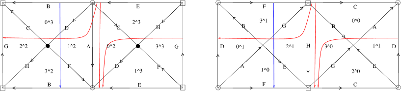
Figure 30. The triangulations of the boundary components, with the branching $\displaystyle\partial\omega_{0}$.

Doing similarly with each of the five other branchings $\displaystyle\partial\omega_{j}$, we find that the surfaces generating $\displaystyle H^{+}(T,\omega_{j})$, $\displaystyle j\in\{1,4\}$, are bounded by (a curve isotopic to) $\displaystyle-\lambda_{1}$, and those generating $\displaystyle H^{+}(T,\omega_{j})$, $\displaystyle j\in\{2,3\}$, are bounded by $\displaystyle\lambda_{0}$. Let us denote them $\displaystyle b$ and $\displaystyle c$ respectively. A surface fully carried by $\displaystyle(T,\omega_{0})$ is given by $\displaystyle b=c=e=g=h=1$, which gives $\displaystyle a=d=3$ and $\displaystyle f=1$. It is bounded by the curves $\displaystyle\mu_{0}+3\lambda_{0}$ and $\displaystyle-2\mu_{1}-2\lambda_{1}$, and so its class $\displaystyle a\in H_{2}(M,\partial M;\mathbb{Z})\cong H_{1}(L;\mathbb{Z})$ has the coordinates $\displaystyle(3,-2)$ in the basis $\displaystyle(\lambda_{0},\lambda_{1})$. Similarly, the class $\displaystyle d$ of the surface fully carried by $\displaystyle(T,\omega_{0})$ given by $\displaystyle a=b=c=d=e=1$ has the coordinates $\displaystyle(-2,-3)$.

The classes $\displaystyle a$, $\displaystyle b$, $\displaystyle c$ and $\displaystyle d$ and the Thurston ball $\displaystyle B_{M}$ (determined in [30]) are shown in Figure 31. The classes $\displaystyle b$ and $\displaystyle c$ are vertices of the Thurston ball $\displaystyle B_{M}$ of $\displaystyle M$; $\displaystyle a$ and $\displaystyle d$ lie in the cones over two distinct and non opposite faces of $\displaystyle B_{M}$. The classes obtained from them by totally reversing the pre-branchings lie in the opposite vertices and fibered faces, respectively.

Figure 31. $\displaystyle B_{M}$ and a few classes of surfaces carried by one of the taut triangulations.

Cohomological invariants. One obtains immediately the weight of the canonical charge $\displaystyle c^{j}$ of the taut triangulation $\displaystyle(T,\omega_{j})$ by looking at Figure 30, for $\displaystyle j=0$, and the analogous figures corresponding to the branchings $\displaystyle\partial\omega_{j}$, $\displaystyle j\in\{1,\ldots,5\}$ (the corners corresponding to diagonal edges, hence where $\displaystyle c^{j}=1$, have one incoming edge and one outgoing edge on the boundary of the triangle it belongs to). We get:

• $\displaystyle k_{c^{0}}$ is identically $\displaystyle 0$;

• $\displaystyle k_{c^{1}}(\mu_{0})=k_{c^{1}}(\mu_{1})=k_{c^{1}}(\lambda_{1})=0$ and $\displaystyle k_{c^{1}}(\lambda_{0})=2$;

• $\displaystyle k_{c^{2}}(\mu_{0})=k_{c^{2}}(\mu_{1})=k_{c^{2}}(\lambda_{0})=0$ and $\displaystyle k_{c^{2}}(\lambda_{1})=2$;

• $\displaystyle k_{c^{3}}(\mu_{0})=k_{c^{3}}(\mu_{1})=0$, $\displaystyle k_{c^{3}}(\lambda_{0})=-1$ and $\displaystyle k_{c^{3}}(\lambda_{1})=-2$;

• $\displaystyle k_{c^{4}}(\mu_{0})=k_{c^{4}}(\mu_{1})=k_{c^{4}}(\lambda_{1})=0$ and $\displaystyle k_{c^{4}}(\lambda_{0})=-2$;

• $\displaystyle k_{c^{5}}$ is identically $\displaystyle 0$;

Hence the the invariants $\displaystyle\partial\mathfrak{h}(*)$ do not distinguish $\displaystyle(T,\omega_{0})$ from $\displaystyle(T,\omega_{5})$.

The symmetry defects. They are given on $\displaystyle(T,\omega_{j})$ as functions of the charge $\displaystyle c$ and the system $\displaystyle{\bf w}$ of quantum shape parameters. Assuming that we take compatible weak branchings $\displaystyle\tilde{b}_{j}$ normalized so that $\displaystyle*_{b}=1$ for each tetrahedron, the edge relations satisfied by $\displaystyle c$ and $\displaystyle{\bf w}$ are (first comes the equation associated to the edges $\displaystyle\bullet$ or with no symbol, and then comes the one for the edges $\displaystyle\circ$ or $\displaystyle\otimes$; see the relations before (8) in Section 8)

$${\bf w}^{2}_{0}{\bf w}^{0}_{2}{\bf w}^{1}_{2}{\bf w}^{3}_{0}=e^{-\frac{2i\pi}{N}}\quad,\quad({\bf w}^{0}_{0})^{2}{\bf w}^{1}_{1}{\bf w}^{2}_{2}{\bf w}^{3}_{2}({\bf w}^{1}_{0})^{2}{\bf w}^{0}_{1}=e^{-\frac{2i\pi}{N}}$$

and

$$c^{2}_{0}+c^{0}_{2}+c^{1}_{2}+c^{3}_{0}=2\quad,\quad 2c^{0}_{0}+c^{1}_{1}+c^{2}_{2}+c^{3}_{2}+2c^{1}_{0}+c^{0}_{1}=2.$$

Besides these relations, there are also the tetrahedral ones, $\displaystyle c^{k}_{0}+c^{k}_{1}+c^{k}_{2}=1$, $\displaystyle k\in\{0,\ldots,3\}$, and $\displaystyle{\bf w}^{k}_{0}{\bf w}^{k}_{1}{\bf w}^{k}_{2}=-e^{\pi/N}$. We see that the gluing variety of shape parameters has complex dimension $\displaystyle 2$, and that the rank of the lattice of charges with given bulk and boundary weights $\displaystyle h_{c}$ and $\displaystyle k_{c}$ is equal to $\displaystyle 2=4\cdot(2{\rm\ charges\ per\ tetrahedron})-(2\ {\rm edge\ relations})-(4\ {\rm weight\ relations})$.

Let us denote by $\displaystyle{\mathcal{T}}_{j}=(T,\tilde{b}_{j},w,f,c)$ a QH triangulation of $\displaystyle M$ supported by $\displaystyle T$ with induced pre-branching $\displaystyle\omega_{j}$. By using the tetrahedral relations and comparing the decorations $\displaystyle d_{j}$ as viewed from the different boundary branched triangulations $\displaystyle(\partial T,\partial\omega_{j})$, we get easily (we put $\displaystyle\zeta:=\exp(2i\pi/N)$):

$$\alpha_{N}({\mathcal{T}}_{0})\alpha_{N}({\mathcal{T}}_{5})^{-1}=\left(\frac{{\bf w}^{2}_{1}{\bf w}^{3}_{1}}{{\bf w}^{0}_{0}{\bf w}^{1}_{0}}(-\zeta^{\frac{N-1}{2}})^{c^{0}_{0}+c^{1}_{0}-c^{2}_{1}-c^{3}_{1}}\right)^{\frac{N-1}{2}}$$

$$\alpha_{N}({\mathcal{T}}_{0})\alpha_{N}({\mathcal{T}}_{1})^{-1}=\left(\frac{{\bf w}^{1}_{1}{\bf w}^{2}_{1}}{{\bf w}^{3}_{0}}(-\zeta^{\frac{N-1}{2}})^{c^{3}_{0}-c^{1}_{1}-c^{2}_{1}}\right)^{\frac{N-1}{2}}$$

$$\alpha_{N}({\mathcal{T}}_{0})\alpha_{N}({\mathcal{T}}_{2})^{-1}=\left(\frac{{\bf w}^{1}_{1}{\bf w}^{3}_{1}}{{\bf w}^{2}_{0}}(-\zeta^{\frac{N-1}{2}})^{c^{2}_{0}-c^{1}_{1}-c^{3}_{1}}\right)^{\frac{N-1}{2}}$$

and so on. By specializing at the complete structure, for instance, where $\displaystyle w^{2}_{0}=w^{0}_{2}=w^{1}_{2}=w^{3}_{0}=i$, and choosing some charge and flattening, one can verify easily that the values are $\displaystyle\neq 1$, so that the symmetry defects distinguish the taut structures defined by the $\displaystyle\omega_{j}$’s.

10. Appendix: The reduced Turaev-Viro invariants

The construction of reduced Turaev-Viro (TV) invariants is much simpler than that of reduced QHI, because their arguments are just compact connected oriented $\displaystyle 3$-manifolds $\displaystyle M$, possibly with non empty boundary. Indeed we slightly modify our set up as follows:

• We consider only oriented compact $\displaystyle 3$-manifolds $\displaystyle M$ with non empty boundary, and we stipulate that either $\displaystyle\partial M$ has no spherical component, or $\displaystyle\partial M$ is connected and consists of one spherical boundary component. The closed manifolds are covered by this latter case.

• We use ideal triangulations of $\displaystyle\hat{M}$, hence we exclude the bubble move.

• We deal with the TV invariants of manifolds with boundary already considered in [10] (where they were related to the Witten-Reshetikhin-Turaev invariants of the “double” $\displaystyle D(M)$), and recently reconsidered in [15].

Let us recall the main features of these invariants. Fix an integer level $\displaystyle r\geq 3$, and $\displaystyle q_{0}$ such that $\displaystyle q:=q_{0}^{2}$ is a primitive $\displaystyle r$th root of $\displaystyle 1$. We have the set of half integer colors

$$I_{r}=\{0,1/2,1,3/2,\cdots,(r-3)/2,(r-2)/2\}.$$

For every positive real number $\displaystyle x$, we denote by $\displaystyle x^{1/2}$ the positive square root; then for $\displaystyle x<0$ we have $\displaystyle x^{1/2}=\sqrt{-1}|x|^{1/2}$. For every integer $\displaystyle m\geq 1$, set

$$[m]=\frac{q_{0}^{m}-q_{0}^{-m}}{q_{0}-q_{0}^{-1}}\in\mathbb{R}\ ,\ [m]!=[m][m-1]\cdots[1].$$

For every $\displaystyle j\in I_{r}$, set

$$w_{j}=\sqrt{-1}^{2j}[2j+1]^{1/2}\ ,\ w=\sqrt{2r}/|q_{0}-q_{0}^{-1}|.$$

A $\displaystyle r$-TV-tetrahedron $\displaystyle(\Delta,b,\sigma)$ consists of:

• A branched tetrahedron $\displaystyle(\Delta,b)$.

• An $\displaystyle I_{r}$-coloring $\displaystyle\sigma$ of the edges of $\displaystyle\Delta$. We require furthermore that $\displaystyle\sigma$ is admissible, that is:

  For every $\displaystyle 2$-face $\displaystyle F$, the sum of the colors of the edges of $\displaystyle F$ is $\displaystyle\leq r-2$, and the colors satisfy all triangular inequalities.

As usual, the branching $\displaystyle b$ corresponds to an ordering $\displaystyle v_{0},v_{1},v_{2},v_{3}$ of the vertices of $\displaystyle\Delta$. If $\displaystyle F_{k}$ is the $\displaystyle 2$-face opposite to the vertex $\displaystyle v_{k}$, then the edges of $\displaystyle F_{k}$ are ordered as usual: $\displaystyle e_{0,k}=[v_{s},v_{t}]$, $\displaystyle e_{1,k}=[v_{t},v_{h}]$, $\displaystyle e_{2,k}=[v_{s},v_{h}]$, where $\displaystyle s<t<h\in\{0,1,2,3\}\setminus\{k\}$. We will denote by $\displaystyle\sigma_{i,j}$ the color that $\displaystyle\sigma$ gives to the edge $\displaystyle e_{i,j}$.

The basic $\displaystyle 6j$-symbol $\displaystyle S_{q_{0}}(\Delta,b,\sigma)$ is a scalar denoted by

$$S_{q_{0}}(\Delta,b,\sigma):=\begin{Bmatrix}\sigma_{2,3}&\sigma_{1,2}&\sigma_{1,3}\\ \sigma_{0,1}&\sigma_{0,3}&\sigma_{0,2}\end{Bmatrix}.$$

It is not important to give here the explicit formula, which is derived from the representation theory of the “small” quantum group $\displaystyle\overline{U}_{q}(sl_{2}(\mathbb{C}))$ (see [31]). Figure 32 shows four branched tetrahedra that share a same pre-branching and carry the $\displaystyle 6j$-symbol

$$\begin{Bmatrix}u&t&m\\ s&p&n\end{Bmatrix}.$$

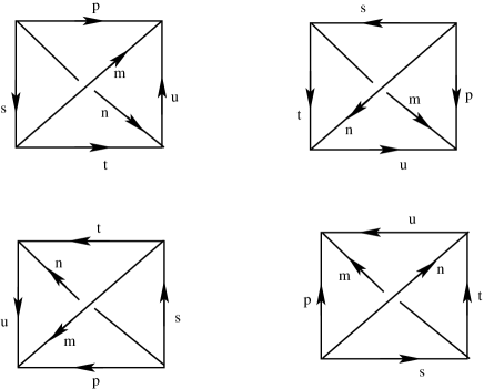
Figure 32. $\displaystyle I$-labelling of $\displaystyle(\Delta,b)$.

The symmetrized $\displaystyle 6j$-symbol $\displaystyle Z_{q_{0}}(\Delta,b,\sigma)$ is defined by:

(17) $$Z_{q_{0}}(\Delta,b,\sigma):=\begin{vmatrix}\sigma_{2,3}&\sigma_{1,2}&\sigma_{1,3}\\ \sigma_{0,1}&\sigma_{0,3}&\sigma_{0,2}\end{vmatrix}:=(w_{\sigma_{0,2}}w_{\sigma_{1,3}})^{-1}\begin{Bmatrix}\sigma_{2,3}&\sigma_{1,2}&\sigma_{1,3}\\ \sigma_{0,1}&\sigma_{0,3}&\sigma_{0,2}\end{Bmatrix}.$$

Here, by “symmetrized” we mean that the value of $\displaystyle Z_{q_{0}}(\Delta,b,\sigma)$ is the same for any branching $\displaystyle b$ on $\displaystyle\Delta$.

A $\displaystyle r$-TV-triangulation $\displaystyle{\mathcal{T}}=(T,\tilde{b},\sigma)$ of $\displaystyle\hat{M}$ consists of a weakly branched triangulation $\displaystyle(T,\tilde{b})$ equipped with an $\displaystyle I_{r}$-coloring $\displaystyle\sigma$ of the edges of $\displaystyle T^{(1)}$, such that every branched tetrahedron $\displaystyle(\Delta,b)$ of $\displaystyle(T,\tilde{b})$ inherits a structure of $\displaystyle r$-TV-tetrahedron. Each $\displaystyle\sigma$ is also called a $\displaystyle r$-state of $\displaystyle(T,\tilde{b})$. Clearly, for every $\displaystyle(T,\tilde{b})$ there is only a finite number of $\displaystyle r$-TV-triangulations $\displaystyle(T,\tilde{b},\sigma)$. Define the TV state sum and the reduced TV state sum by

(18) $$\textstyle|T,\tilde{b}|_{q_{0}}:=\sum_{\sigma}\left(\prod_{e\in T^{(1)}}w_{\sigma(e)}^{2}\right)\ Z_{q_{0}}(T,\tilde{b},\sigma)$$

$$\textstyle|T,\tilde{b}|^{{\rm red}}_{q_{0}}:=\sum_{\sigma}S_{q_{0}}(T,\tilde{b},\sigma)$$

where

$$Z_{q_{0}}(T,\tilde{b},\sigma)=\prod_{\Delta\in T^{(3)}}Z_{q_{0}}(\Delta,b,\sigma)\ ,\ S_{q_{0}}(T,\tilde{b},\sigma)=\prod_{\Delta\in T^{(3)}}S_{q_{0}}(\Delta,b,\sigma)$$

and $\displaystyle\sigma$ ranges over the set of $\displaystyle r$-states of $\displaystyle(T,\tilde{b})$.

Remark 10.1.

There is an important difference between the TV and the QHI local symmetrization factors. In the TV case, they are the scalars $\displaystyle\alpha_{q_{0}}(\Delta,b,\sigma):=(w_{\sigma_{0,2}}w_{\sigma_{1,3}})^{-1}$ in (17), which depend on the $\displaystyle r$-state $\displaystyle\sigma$. This and the factor $\displaystyle\textstyle\prod_{e\in T^{(1)}}w_{\sigma(e)}^{2}$ in (18) imply that it is no longer true that the state sums $\displaystyle|T,\tilde{b}|_{q_{0}}$ differ from the reduced ones $\displaystyle|T,\tilde{b}|^{{\rm red}}_{q_{0}}$ just by a global symmetrization factor.

The naked ideal triangulation moves can be enhanced automatically to TV-transits $\displaystyle(T,\tilde{b},\sigma)\leftrightarrow(T^{\prime},\tilde{b}^{\prime},\sigma^{\prime})$, defined by imposing that $\displaystyle\sigma^{\prime}$ and $\displaystyle\sigma$ coincide on the common edges of $\displaystyle T$ and $\displaystyle T^{\prime}$. The main result of [31] is that

$$|M|_{q_{0}}:=|T,\tilde{b}|_{q_{0}}$$

is a well defined real valued topological invariant of $\displaystyle M$. The proof is based on the fact that the TV state sums are fully TV-transit invariant.

Remark 10.2.

The choice of $\displaystyle q_{0}$, and not only $\displaystyle r$, is far to be immaterial. For example, if $\displaystyle r$ is odd, both $\displaystyle q_{0}=\exp(i\pi/r)$ and $\displaystyle q_{0}=\exp(2i\pi/r)$ are possible choices. Let $\displaystyle M$ have non trivial boundary, eg. take $\displaystyle M=M_{8}$ as in Section 9. In [15] one can find evidences that, for the first choice of $\displaystyle q_{0}$, $\displaystyle|M|_{q_{0}}$ has polynomial growth when $\displaystyle r$ is odd and $\displaystyle r\to+\infty$, accordingly with the Witten asymptotic expansion conjecture for the Witten-Reshetikhin-Turaev invariant $\displaystyle WRT_{q_{0}}(D(M))$ of the double of $\displaystyle M$ (see [10]). On the other hand, $\displaystyle|M|_{q_{0}}$ grows exponentially for the second choice of $\displaystyle q_{0}$.

We can formulate the analog of Theorem 1.6 as follows.

Theorem 10.3.

(1) For every ideal triangulation $\displaystyle(T,\tilde{b})$ of $\displaystyle\hat{M}$, the value of the reduced state sum $\displaystyle|T,\tilde{b}|_{q_{0}}^{{\rm red}}$ depends only the underlying pre-branched triangulation $\displaystyle(T,\omega_{\tilde{b}})$. Moreover, it is invariant under the total inversion of the pre-branchings.

(2) If $\displaystyle(T,\tilde{b})$ and $\displaystyle(T^{\prime},\tilde{b}^{\prime})$ are ideal triangulations of $\displaystyle\hat{M}$ such that $\displaystyle(T,\omega_{\tilde{b}})$ and $\displaystyle(T^{\prime},\omega_{\tilde{b}^{\prime}})$ represent the same non ambiguous structure on $\displaystyle M$, say $\displaystyle{\mathfrak{s}}$, then $\displaystyle|T,\tilde{b}|_{q_{0}}^{{\rm red}}=|T^{\prime},\tilde{b}^{\prime}|_{q_{0}}^{{\rm red}}$.

Hence there are well defined reduced TV invariants $\displaystyle|M;{\mathfrak{s}}|^{{\rm red}}_{q_{0}}$, which are invariant under the natural total inversion involution on the set of non ambiguous structures.

Proof. A change of the weak branching that preserves or reverses totally the pre-branching does not modify the TV local symmetrization factors, because $\displaystyle(w_{\sigma_{0,2}}w_{\sigma_{1,3}})^{-1}$ does not depend on the colors of the square edges. So Theorem 10.3 (1) follows immediately.

As for the TV transits, let us just consider the $\displaystyle 2\rightarrow 3$ one (things are similar with the lune move). It is enough to prove that

(19) $$S_{q_{0}}(T,b,\sigma)=\sum_{\sigma^{\prime}}S_{q_{0}}(T^{\prime},b^{\prime},\sigma^{\prime})$$

whenever $\displaystyle(T,b)\to(T^{\prime},b^{\prime})$ is one of the two remarkable $\displaystyle b$-transits described before Lemma 3.5, and the move $\displaystyle(T,b,\sigma)\rightarrow(T^{\prime},b^{\prime},\sigma^{\prime})$ varies among its TV enhancements. We realize that (19) is the Biedenharn-Elliot identity that arises from the representations theory of $\displaystyle\overline{U}_{q}(sl_{2}(\mathbb{C}))$. This achieves also Theorem 10.3 (2). $\displaystyle\Box$

It is interesting to recover the proof of Theorem 10.3 (2) in a way which points out also a holographic content, in the sense of what we have developed in Section 5. Every triple $\displaystyle(T,\omega,\sigma)$ as above restricts naturally to a boundary “TV branched triangulation” $\displaystyle(\partial T,\partial\omega,\partial\sigma)$, where $\displaystyle\partial\sigma$ is the $\displaystyle I_{r}$-coloring of the vertices of $\displaystyle\partial T$ induced by $\displaystyle\sigma$. For every such a colored $\displaystyle 2D$ branched triangulation $\displaystyle(\partial T,\partial\omega,\partial\sigma)$ and every vertex $\displaystyle v$ of $\displaystyle\partial T$, let $\displaystyle C_{v}$ be the $\displaystyle 2$-cell dual to $\displaystyle v$. Define

$$\alpha_{TV}(\partial T,\partial\omega,\partial\sigma)=\prod_{v\in\partial T}w_{\partial\sigma(v)}^{{\rm Eu}_{b}(C_{v})}.$$

A simple rewriting of the formulas shows that:

Lemma 10.4.

For every TV-triangulation $\displaystyle(T,\tilde{b},\sigma)$ of $\displaystyle\hat{M}$ we have

$$Z_{q_{0}}(T,\tilde{b},\sigma)=\alpha_{TV}(\partial T,\partial\omega_{\tilde{b}},\partial\sigma)S_{q_{0}}(T,\tilde{b},\sigma).$$

Hence $\displaystyle\alpha_{TV}(\partial T,\partial\omega_{\tilde{b}},\partial\sigma)$ can be considered as the symmetrization factor of the product of basic $\displaystyle 6j$-symbols $\displaystyle S_{q_{0}}(T,\tilde{b},\sigma)$, and is entirely determined by the boundary TV triangulation. Now, in the remarkable $\displaystyle b$-transits described before Lemma 3.5, for every $\displaystyle\sigma^{\prime}$ we have

$$\alpha_{TV}(\partial T^{\prime},\partial\omega^{\prime},\partial\sigma^{\prime})=\alpha_{TV}(\partial T,\partial\omega,\partial\sigma).$$

So, up to an overall scalar factor, the Biedenharn-Elliot identity (19) coincides with the identity obtained from it by replacing $\displaystyle S_{q_{0}}$ with $\displaystyle Z_{q_{0}}$. Ultimately, this depends on the nice behaviour of the scalar $\displaystyle\alpha_{TV}(\partial T,\partial\omega,\partial\sigma)$ under $\displaystyle 2D$ sliding transits.

Finally, recall that the taut structures are in a sense the most natural non ambiguous structures. To this respect we note that the reduced TV invariants are disappointing. In fact $\displaystyle\alpha_{TV}(\partial T,\partial\omega,\partial\sigma)=1$ for a taut triangulation $\displaystyle(T,\omega)$. Hence:

Corollary 10.5.

For every taut structure $\displaystyle{\mathfrak{s}}$ on $\displaystyle M$ we have $\displaystyle|M;{\mathfrak{s}}|^{{\rm red}}_{q_{0}}=|M|_{q_{0}}$.

So the reduced TV invariants are completely blind with respect to the taut structures (though they can distinguish other non ambiguous structures on $\displaystyle M$). This can be regarded as a TV counterpart of the fact that the QHI symmetrization factors $\displaystyle\alpha_{N}(T,\tilde{b},w,f,c)=1$, whenever $\displaystyle(T,\omega_{\tilde{b}})$ is a taut triangulation and $\displaystyle c$ is the tautological charge carried by $\displaystyle(T,\omega_{\tilde{b}})$. The advantage of the QH framework is that we can vary also the $\displaystyle c$-weight $\displaystyle k_{c}$ in order to distinguish different taut structures, as we have done in Section 9.

On the other hand, recall that the normalized QH symmetry defects are blind with respect to the relative non ambiguous structures on $\displaystyle(M,L)$. The situation for reduced TV invariants is slightly better in the relative case. Let us work for example with relative taut triangulations $\displaystyle(T,H,\omega)$ of $\displaystyle(M,L)$ (if any) and the corresponding relative taut structures $\displaystyle{\mathfrak{s}}$. Then the reduced TV invariant $\displaystyle|M,L;{\mathfrak{s}}|^{\rm red}_{q_{0}}$ does not coincide in general with $\displaystyle|M|_{q_{0}}$, and it should be sensitive to both $\displaystyle L$ and $\displaystyle{\mathfrak{s}}$. As an example, let us outline a construction of invariants of fibred knots $\displaystyle K$ in $\displaystyle S^{3}$. Let $\displaystyle Y$ be the complement of an open tubular neighbourhood of $\displaystyle K$ in $\displaystyle S^{3}$. Let $\displaystyle M$ be obtained via Dehn filling of $\displaystyle Y$ along the canonical longitude, say $\displaystyle m$, of $\displaystyle K$, and $\displaystyle L\subset M$ be the core of the attached solid torus. Since $\displaystyle Y$ has a single fibration it has a canonical taut structure $\displaystyle{\mathfrak{s}}_{Y}$. By Section 7 it extends to a relative taut structure $\displaystyle{\mathfrak{s}}_{K}$ on $\displaystyle(M,L)$. Hence $\displaystyle|M,L;{\mathfrak{s}}_{K}|^{{\rm red}}_{q_{0}}$ is an invariant of the fibred knot $\displaystyle K$.

References

- [1] I. Agol, Ideal Triangulations of Pseudo-Anosov Mapping Tori, in Topology and geometry in dimension three, Amer. Math. Soc. Contemp. Math. Vol 560 (2011), 1–17
- [2] I. Agol, http://mathoverflow.net/questions/106426/comparing-layered-triangulations-of-3-manifolds-which-fiber-over-the-circle
- [3] G. Amendola, A calculus for ideal triangulations of three-manifolds with embedded arcs, Math. Nachr. 278 (9) (2005) 975–994
- [4] S. Baseilhac, R. Benedetti, Quantum Hyperbolic invariants of 3-manifolds with -characters, Topology 43 (6) (2004) 1373–1423
- [5] S. Baseilhac, R. Benedetti, Classical and quantum dilogarithmic invariants of flat -bundles over -manifolds, Geom. Topol. 9 (2005) 493–570
- [6] S. Baseilhac, R. Benedetti, Quantum hyperbolic geometry, Alg. Geom. Topol. 7 (2007) 845–917
- [7] S. Baseilhac, R. Benedetti, The Kashaev and quantum hyperbolic link invariants, Journal GGT 5 (2011) 31–85
- [8] S. Baseilhac, R. Benedetti, Analytic families of quantum hyperbolic invariants, Alg. Geom. Topol. 15 (2015) 1983–2063.
- [9] H. Bai, F. Bonahon, X. Liu, Local representations of the quantum Teichmüller space, preprint, ArXiv:0707.2151 (2007)
- [10] R. Benedetti, C. Petronio, On Roberts’ proof of the Turaev-Walker theorem, Journal of Knot Theory and its Ramifications 5 (4) (1996) 427–439
- [11] R. Benedetti, C. Petronio, Branched Standard Spines of -manifolds, Lect. Notes Math. 1653, Springer (1997)
- [12] R. Benedetti, C. Petronio, Reidemeister-Turaev torsion of 3-dimensional Euler structures with simple boundary tangency and pseudo-Legendrian knots, Manuscripta Math. 106 (1) (2001) 13–61
- [13] R. Benedetti, C. Petronio, Spin structures on -manifolds via arbitrary triangulations, Alg. Geom. Topol. 14 (2014) 1005–1054
- [14] B. A. Burton, R. Budney, W. Pettersson, et al., Regina: Software for 3-manifold topology and normal surface theory, http://regina.sourceforge.net, 1999-2014
- [15] Q. Chen, T. Yang, A volume conjecture for a family of Turaev-Viro type invariants of -manifolds with boundary, preprint, ArXiv:1503.02547 (2015)
- [16] M. Culler, N. M. Dunfield, J. R. Weeks, SnapPy, a computer program for studying the geometry and topology of 3-manifolds, http://snappy.computop.org
- [17] N. Dunfield, Cyclic surgery, degree of maps of character curves, and volume rigidity for hyperbolic manifolds, Invent. Math. 136 (1999) 623–657
- [18] D. Fried, Fibrations over with pseudo-Anosov monodromy, Exposé 14 in “Travaux de Thurston sur les surfaces” by A. Fathi, F. Laudenbach and V. Poenaru, Astérisque 66-67, Société Mathématique de France (1979) 251–266
- [19] F. Guéritaud, D. Futer, Explicit angle structures for veering triangulations, Alg. Geom. Topol. 13 (2013) 205–235
- [20] S. Halperin, D. Toledo, Stiefel-Whitney homology classes, Ann. of Math. (2) 96 (1972) 511–525
- [21] A. Hatcher, Algebraic Topology, Cambridge University Press, 2002
- [22] C.D. Hogdson, J.H. Rubinstein, H. Segerma,, S. Tillman, Veering triangulations admit strict angle structures, Geom. Topol. 15 (2011) 2073–2089
- [23] I. Ishii, Flows and spines, Tokyo J. Math. 9 (1986) 505–525
- [24] R.M. Kashaev, Quantum dilogarithm as a -symbol, Mod. Phys. Lett. A Vol. 9, No 40 (1994) 3757–3768
- [25] B. Klaff, S. Tillmann, A birationality result for character varieties, to appear in Math. Res. Letters, ArXiv:13096010
- [26] M. Lackenby, Taut ideal triangulations of -manifolds, Geom. Topol. 4 (2000) 369–395
- [27] H. Masur, J. Smillie, Quadratic differentials with prescribed singularities and pseudo-Anosov diffeomorphisms, Commentari Math. Helvetici 68 (1993) 289–307
- [28] W.D. Neumann, Combinatorics of triangulations and the Chern-Simons invariant for hyperbolic -manifolds, Topology ’90 (Columbus, OH, 1990), De Gruyter, Berlin (1992) 243–271
- [29] M. Scharlemann , Sutured manifolds and generalized Thurston norms, J. Diff. Geom. 29 (1989) 577– 614
- [30] W. Thurston, A norm on the homology of three-manifolds, Mem. Amer. Math. Soc. 339 (1986) 99–130
- [31] V. Turaev, O. Viro, State sum invariants of 3-manifolds and quantum 6j-symbols, Topology 31 (4) (1992) 865–902
- [32] V. Turaev, Quantum Invariants of Knots and 3-manifolds, De Gruyter Studies in Math. 18 (1994)