A new model to predict weak-lensing peak counts

Abstract

Context. Peak counts have been shown to be an excellent tool for extracting the non-Gaussian part of the weak lensing signal. Recently, we developed a fast stochastic forward model to predict weak-lensing peak counts. Our model is able to reconstruct the underlying distribution of observables for analysis.

Aims. In this work, we explore and compare various strategies for constraining a parameter using our model, focusing on the matter density $\Omega_{\mathrm{m}}$ and the density fluctuation amplitude $\sigma_{8}$.

Methods. First, we examine the impact from the cosmological dependency of covariances (CDC). Second, we perform the analysis with the copula likelihood, a technique that makes a weaker assumption than does the Gaussian likelihood. Third, direct, non-analytic parameter estimations are applied using the full information of the distribution. Fourth, we obtain constraints with approximate Bayesian computation (ABC), an efficient, robust, and likelihood-free algorithm based on accept-reject sampling.

Results. We find that neglecting the CDC effect enlarges parameter contours by 22% and that the covariance-varying copula likelihood is a very good approximation to the true likelihood. The direct techniques work well in spite of noisier contours. Concerning ABC, the iterative process converges quickly to a posterior distribution that is in excellent agreement with results from our other analyses. The time cost for ABC is reduced by two orders of magnitude.

Conclusions. The stochastic nature of our weak-lensing peak count model allows us to use various techniques that approach the true underlying probability distribution of observables, without making simplifying assumptions. Our work can be generalized to other observables where forward simulations provide samples of the underlying distribution.

1 Introduction

Weak lensing (WL) is a gravitational deflection effect of light by matter inhomogeneities in the Universe that causes distortion of source galaxy images. This distortion corresponds to the integrated deflection along the line of sight, and its measurement probes the high-mass regions of the Universe. These regions contain structures that formed during the late-time evolution of the Universe, which depends on cosmological parameters, such as the matter density parameter $\Omega_{\mathrm{m}}$, the matter density fluctuation $\sigma_{8}$, and the equation of state of dark energy $w$. Ongoing and future surveys such as KiDS , DES , HSC , WFIRST , Euclid , and LSST are expected to provide tight constraints on those and other cosmological parameters and to distinguish between different cosmological models, using weak lensing as a major probe.

Lensing signals can be extracted in several ways. A common observable is the cosmic shear two-point-correlation function (2PCF), which has been used to constrain cosmological parameters in many studies, including recent ones (Kilbinger_etal_2013; Jee_etal_2013). However, the 2PCF only retains Gaussianity, and it misses the rich nonlinear information of the structure evolution encoded on small scales. To compensate for this drawback, several non-Gaussian statistics have been proposed, for example higher order moments (Kilbinger_Schneider_2005; Semboloni_etal_2011; Fu_etal_2014; Simon_etal_2015), the three-point correlation function (Schneider_Lombardi_2003; Takada_Jain_2003; Scoccimarro_etal_2004), Minkowski functionals (Petri_etal_2015), or peak statistics, which is the aim of this series of papers. Some more general work comparing different strategies to extract non-Gaussian information can be found in the literature (Pires_etal_2009a; Berge_etal_2010; Pires_etal_2012).

Peaks, defined as local maxima of the lensing signal, are direct tracers of high-mass regions in the large-scale structure of the Universe. In the medium and high signal-to-noise (S/N) regime, the peak function (the number of peaks as function of S/N) is not dominated by shape noise, and this permits one to study the cosmological dependency of the peak number counts (Jain_VanWaerbeke_2000). Various aspects of peak statistic have been investiagated in the past: the physical origin of peaks (Hamana_etal_2004; Yang_etal_2011), projection effects (Marian_etal_2010), the optimal combination of angular scales (Kratochvil_etal_2010; Marian_etal_2012), redshift tomography (Hennawi_Spergel_2005), cosmological parameter constraints (Dietrich_Hartlap_2010; Liu_etal_2014), detecting primordial non-Gaussianity (Maturi_etal_2011; Marian_etal_2011), peak statistics beyond the abundance (Marian_etal_2013), the impact from baryons (Yang_etal_2013; Osato_etal_2015), magnification bias (Liu_etal_2014a), and shape measurement errors (Bard_etal_2013). Recent studies by Liu_etal_2015 (Liu_etal_2015, hereafterLiu_etal_2015), Liu_etal_2015a (Liu_etal_2015a, hereafterLiu_etal_2015a), and Hamana_etal_2015 have applied likelihood estimation for WL peaks on real data and have shown that the results agree with the current $\Lambda$CDM scenario.

Modeling number counts is a challenge for peak studies. To date, there have been three main approaches. The first one is to count peaks from a large number of $N$-body simulations (Dietrich_Hartlap_2010; Liu_etal_2015), which directly emulate structure formation by numerical implementation of the corresponding physical laws. The second family consists of analytic predictions (Maturi_etal_2010; Fan_etal_2010) based on Gaussian random field theory. A third approach has been introduced by Lin_Kilbinger_2015: Similar to Kruse_Schneider_1999 and Kainulainen_Marra_2009; Kainulainen_Marra_2011; Kainulainen_Marra_2011a, we propose a stochastic process to predict peak counts by simulating lensing maps from a halo distribution drawn from the mass function.

Our model possesses several advantages. The first one is flexibility. Observational conditions can easily be modeled and taken into account. The same is true for additional features, such as intrinsic alignment of galaxies and other observational and astrophysical systematics. Second, since our method does not need $N$-body simulations, the computation time required to calculate the model are orders of magnitudes faster, and we can explore a large parameter space. Third, our model explores the underlying probability density function (PDF) of the observables. All statistical properties of the peak function can be derived directly from the model, making various parameter estimation methods possible.

In this paper, we apply several parameter constraint and likelihood methods for our peak-count-prediction model from Lin_Kilbinger_2015. Our goal is to study and compare different strategies and to make use of the full potential of the fast stochastic forward modeling approach. We start with a likelihood function that is assumed to be Gaussian in the observables with constant covariance and then compare this to methods that make fewer and fewer assumptions, as follows.

The first extension of the Gaussian likelihood is to take the cosmology-dependent covariances (CDC, see Eifler_etal_2009) into account. Thanks to the fast performance of our model, it is feasible to estimate the covariance matrix for each parameter set.

The second improvement we adopt is the copula analysis (Benabed_etal_2009; Jiang_etal_2009; Takeuchi_2010; Scherrer_etal_2010; Sato_etal_2011) for the Gaussian approximation. Widely used in finance, the copula transform uses the fact that any multivariate distribution can be transformed into a new one where the marginal PDF is uniform. Combining successive transforms can then give rise to a new distribution where all marginals are Gaussian. This makes weaker assumptions about the underlying likelihood than the Gaussian hypothesis.

Third, we directly estimate the full underlying distribution information in a non-analytical way. This allows us to strictly follow the original definition of the likelihood estimator: the conditional probability of observables for a given parameter set. In addition, we compute the $p$-value from the full PDF. These $p$-values derived for all parameter sets allow for significance tests and provide a direct way to construct confidence contours.

Furthermore, our model makes it possible to dispose of a likelihood function altogether, using approximate Bayesian computation (ABC, see e.g. Marin_etal_2011) for exploring the parameter space. ABC is a powerful constraining technique based on accept-reject sampling. Proposed first by Rubin_1984, ABC produces the posterior distribution by bypassing the likelihood evaluation, which may be complex and practically unfeasible in some contexts. The posterior is constructed by comparing the sampled result with the observation to decide whether a proposed parameter is accepted. This technique can be improved by combining ABC with population Monte Carlo (PMC , Beaumont_etal_2009; Cameron_Pettitt_2012; Weyant_etal_2013). Until now, ABC seems to already have various applications in biology-related domains (e.g., Beaumont_etal_2009; Berger_etal_2010; Csillery_etal_2010; Drovandi_Pettitt_2011), while applications for astronomical purposes are few: morphological transformation of galaxies (Cameron_Pettitt_2012), cosmological parameter inference using type Ia supernovae (Weyant_etal_2013), constraints of the disk formation of the Milky Way (Robin_etal_2014), and strong lensing properties of galaxy clusters (Killedar_etal_2015). Very recently, two papers (Ishida_etal_2015; Akeret_etal_2015) dedicated to ABC in a general cosmological context have been submitted.

The paper is organized as follows. In Sect. 2, we briefly review our model introduced in Lin_Kilbinger_2015, the setting for the parameter analysis, and the criteria for defining parameter constraints. In Sect. LABEL:sect:CDC, we study the impact of the CDC effect. The results from the copula likelihood can be found in Sect. LABEL:sect:copula, and in Sect. LABEL:sect:nonParam we estimate the true underlying PDF in a non-analytic way and show parameters constraints without the Gaussian hypothesis. Sect. LABEL:sect:ABC focuses on the likelihood-free ABC technique, and the last section is dedicated to a discussion where we summarize this work.

2 Methodology

2.1 Our model

Our peak-count model uses a probabilistic approach that generates peak catalogs from a given mass function model. This is done by generating fast simulations of halos, computing the projected mass, and simulating lensing maps from which one can extract WL peaks. A step-by-step summary is given as follows:

1. sample halo masses and assign density profiles and positions (fast simulations),

2. compute the projected mass and subtract the mean over the field (ray-tracing simulations),

3. add noise and smooth the map with a kernel, and

4. select local S/N maxima.

Here, two assumptions have been made: (1) only bound matter contributes to number counts and (2) the spatial correlation of halos has a small impact on WL peaks. Lin_Kilbinger_2015 showed that combining both hypotheses gives a good estimation of the peak abundance.

Table 1: List of parameter values adopted in this study.

Parameter	Symbol	Value
Lower sampling limit	-	$10^{12}$ $M_{\odot}/h$
Upper sampling limit	-	$10^{17}$ $M_{\odot}/h$
NFW inner slope	$\alpha$	1
$M$-$c$ relation parameter	$c_{0}$	11
$M$-$c$ relation parameter	$\beta$	0.13
Source redshift	$z_{\mathrm{s}}$	1
Intrinsic ellipticity dispersion	$\sigma_{\epsilon}$	0.4
Galaxy number density	$n_{\mathrm{g}}$	25 arcmin${}^{-2}$
Pixel size	$\theta_{\mathrm{pix}}$	0.2 arcmin
Kernel size	$\theta_{\mathrm{G}}$	1 arcmin
Shape noise	$\sigma_{\mathrm{pix}}$	0.283
Smoothed noise	$\sigma_{\mathrm{noise}}$	0.0226
Effective field area	-	25 deg${}^{2}$

We adopt the same settings as Lin_Kilbinger_2015: the mass function model from Jenkins_etal_2001, the truncated Navarro-Frenk-White halo profiles (Navarro_etal_1996; Navarro_etal_1997), Gaussian shape noise, the Gaussian smoothing kernel, and sources at fixed redshift which are distributed on a regular grid. The field of view is chosen such that the effective area after cutting off the border is 25 deg${}^{2}$. An exhausted list of parameter values used in this paper can be found in Table 1. Readers are encouraged to read Lin_Kilbinger_2015 for their definitions and for detailed explanations for our model.

All computations with our model in this study are performed by our Camelus algorithm . A realization (from a mass function to a peak catalog) of a 25-deg${}^{2}$ field costs few seconds to generate on a single-CPU computer. The real time cost depends of course on input cosmological parameters, but this still gives an idea about the speed of our algorithm.

2.2 Analysis design

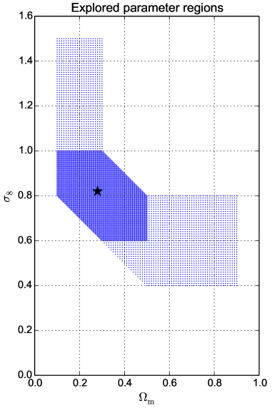
Figure 1: Location of 7821 points on which we evaluate the likelihoods. In the condensed area, the interval between two grid points is 0.005, while in both wing zones it is 0.01. The black star shows $(\Omega_{\mathrm{m}}^{\mathrm{in}},\sigma_{8}^{\mathrm{in}})=(0.28,0.82)$.

Throughout this paper, $\boldsymbol{\pi}$ denotes a parameter set. To simplify the study, the dimension of the parameter space is reduced to two: $\boldsymbol{\pi}\equiv(\Omega_{\mathrm{m}},\sigma_{8})$. The other cosmological parameters are fixed, including $\Omega_{\mathrm{b}}=0.047$, $h=0.78$, $n_{s}=0.95$, and $w=-1$. The dark energy density $\Omega_{\mathrm{d}\mathrm{e}}$ is set to $1-\Omega_{\mathrm{m}}$ to match a flat universe. On the $\Omega_{\mathrm{m}}$-$\sigma_{8}$ plane, we explore a region where the posterior density, or probability, is high, see Fig. 1. We compute the values of three different log likelihoods on the grid points of these zones. The grid size of the center zone is $\Delta\Omega_{\mathrm{m}}=\Delta\sigma_{8}=0.005$, whereas it is 0.01 for the rest. This results in a total of 7821 points in the parameter space to evaluate.

For each $\boldsymbol{\pi}$, we carry out $N=1000$ realizations of a 25-deg${}^{2}$ field and determine the associated data vector $\boldsymbol{x}^{(k)}=(x^{(k)}_{1},\ldots,x^{(k)}_{d})$ for all $k$ from 1 to $N$. These are independent samples drawn from their underlying PDF of observables for a given parameter $\boldsymbol{\pi}$. We estimate the model prediction (which is the mean), the covariance matrix, and the inverse matrix (Hartlap_etal_2007), respectively, by following

$$x^{\mathrm{mod}}_{i} =\frac{1}{N}\sum_{k=1}^{N}x_{i}^{(k)},$$ (1)

$$\hat{C}_{ij} =\frac{1}{N-1}\sum_{k=1}^{N}\left(x_{i}^{(k)}-x^{\mathrm{mod}}_{i}\right)\left(x_{j}^{(k)}-x^{\mathrm{mod}}_{j}\right),\ \ \text{and}$$ (2)

$$\widehat{\boldsymbol{C}^{-1}} =\frac{N-d-2}{N-1}\ \widehat{\boldsymbol{C}}^{-1},$$ (3)

where $d$ denotes the dimension of data vector. This results in a total area of 25 000 deg${}^{2}$ for the mean estimation.

In this paper, the observation data $\boldsymbol{x}^{\mathrm{obs}}$ are identified with a realization of our model, which means that $\boldsymbol{x}^{\mathrm{obs}}$ is derived by a particular realization of $\boldsymbol{x}(\boldsymbol{\pi}^{\mathrm{in}})$. The input parameters chosen are $\boldsymbol{\pi}^{\mathrm{in}}=(\Omega_{\mathrm{m}}^{\mathrm{in}},\sigma_{8}^{\mathrm{in}})=(0.28,0.82)$. The authors would like to highlight that the accuracy of the model is not the aim of this research work, but precision. Therefore, the input choice and the uncertainty of random process should have little impact.

Peak-count information can be combined into a data vector using different ways. Inspired by Dietrich_Hartlap_2010 and Liu_etal_2015a, we studied three types of observables. The first is the abundance of peaks found in each S/N bin (labeled abd), in other words, the binned peak function. The second is the S/N values at some given percentiles of the peak cumulative distribution function (CDF, labeled pct). The third is similar to the second type, but without taking peaks below a threshold S/N value (labeled cut) into account. Mathematically, the two last types of observables can be denoted as $x_{i}$, thereby satisfying

$$p_{i}=\int_{\nu_{\mathrm{min}}}^{x_{i}}n_{\mathrm{peak}}(\nu)\mathrm{d}\nu,$$ (4)

where $n_{\mathrm{peak}}(\nu)$ is the peak PDF function, $\nu_{\mathrm{min}}$ a cutoff, and $p_{i}$ a given percentile. The observable $\boldsymbol{x}^{\mathrm{abd}}$ is used by Liu_etal_2015a, while readers find $\boldsymbol{x}^{\mathrm{cut}}$ from Dietrich_Hartlap_2010. We would like to clarify that using $\boldsymbol{x}^{\mathrm{pct}}$ for analysis could by risky, since this includes peaks with negative S/N. From Lin_Kilbinger_2015, we observe that although high-peak counts from our model agree well with $N$-body simulations, predictions for local maxima found in underdensity regions (peaks with S/N ¡ 0) are inaccurate. Thus, we include $\boldsymbol{x}^{\mathrm{pct}}$ in this paper only to give an idea about how much information we can extract from observables defined by percentiles.

Table 2: Definition of $\boldsymbol{x}^{\mathrm{abd}5}$, $\boldsymbol{x}^{\mathrm{pct}5}$, and $\boldsymbol{x}^{\mathrm{cut}5}$. Parameters such as $\nu_{\mathrm{min}}$ and $p_{i}$ are used by Eq. (4). As an indication, their values for the input cosmology $\boldsymbol{\pi}^{\mathrm{in}}$ are also given. They were calculated by averaging over 1000 realizations.

Label	abd5
Bins on $\nu$	[3.0, 3.8[	[3.8, 4.5[	[4.5, 5.3[	[5.3, 6.2[	[6.2, $+\infty$[
$x_{i}$ for $\pi^{\mathrm{in}}$	330	91	39	18	15
Label	pct5
$\nu_{\mathrm{min}}$	$-\infty$
$p_{i}$	0.969	0.986	0.994	0.997	0.999
$x_{i}$ for $\pi^{\mathrm{in}}$	3.5	4.1	4.9	5.7	7.0
Label	cut5
$\nu_{\mathrm{min}}$	3
$p_{i}$	0.5	0.776	0.9	0.955	0.98
$x_{i}$ for $\pi^{\mathrm{in}}$	3.5	4.1	4.9	5.7	6.7

Observable vectors are constructed by the description above with the settings of Table 2. This choice of bins and $p_{i}$ is made such that the same component from different types of observables represents about the same information, since the bin center of $\boldsymbol{x}^{\mathrm{abd}5}$ roughly correspond to $\boldsymbol{x}^{\mathrm{cut}5}$ for the input cosmology $\boldsymbol{\pi}^{\mathrm{in}}$. Following Liu_etal_2015a, who discovered in their study that the binwidth choice has a minor impact on parameter constraints if the estimated number count in each bin is $\gtrsim$ 10, we chose not to explore different choices of binwidths for $\boldsymbol{x}^{\mathrm{abd}5}$. We also note that $p_{i}$ for $x_{i}^{\mathrm{cut}5}$ are logarithmically spaced.

By construction, the correlation between terms of percentile-like vectors is much higher than for the case of peak abundance. This tendency is shown in Table LABEL:tab:corr_matrices for the $\boldsymbol{\pi}^{\mathrm{in}}$ cosmology. We discovered that $\boldsymbol{x}^{\mathrm{pct}5}$ and $\boldsymbol{x}^{\mathrm{cut}5}$ are highly correlated, while for $\boldsymbol{x}^{\mathrm{abd}5}$, the highest absolute value of off-diagonal terms does not exceed 17%. A similar result was observed when we binned data differently. This suggests that the covariance should be included in likelihood analyses.

Table 3: Correlation matrices of $\boldsymbol{x}^{\mathrm{abd}5}$, $\boldsymbol{x}^{\mathrm{pct}5}$, and $\boldsymbol{x}^{\mathrm{cut}5}$ in the input cosmology. For $\boldsymbol{x}^{\mathrm{abd}5}$, the peak abundance is weakly correlated between bins.

abd5		-0.05	-0.09	-0.08	-0.16
-0.05	1	-0.05	-0.01	-0.12
-0.09	-0.05	1	-0.04	-0.11
-0.08	-0.01	-0