Abstract

The entangled behavior of different dimensional systems driven by classical external random field is investigated. The amount of the survival entanglement between the components of each system is quantified. There are different behaviors of entanglement that come into view decay, sudden death, sudden birth and long-lived entanglement. The maximum entangled states which can be generated from any of theses suggested systems are much fragile than the partially entangled ones. The systems of larger dimensions are more robust than those of smaller dimensions systems, where the entanglement decay smoothly, gradually and may vanish for a very short time. For the class of $2\times 3$ dimensional system, the one parameter family is found to be more robust than the two parameters family. Although the entanglement of driven $2\times 3$ dimensional system is very sensitive to the classical external random field, one can use them to generate a long-lived entanglement.

pacs:03.67.-a, 03.67.Bg, 03.67.Hk keywords:External fields, Qubit, qutrit, Entanglement

1 Introduction

It is well known that, noise represents one of the unavoidable physical phenomena in the context of quantum information and computation. The effect of different types of noises on many systems has been investigated extensively for two dimensional systems, (see for example [1, 2, 3, 4, 5, 6]). The dynamics of higher dimensional systems which travel in different noise channels have been discussed. For example, the separability of entangled qutrits in a noise channel is investigated in [7]. The time evolution of classical and quantum correlations of hybrid qubit-qutrit systems in a classical dephasing environment has been studied [8]. Also, the decoherent dynamics of quantum correlations in qubit-qutrit system under various noise channels has been discussed in [9]. The dynamics of entanglement for a qutrit system in the presence of global, collective, multilocal and local noise channels is studied [10]. The possibility of protecting entanglement in qubit-qutrit system from decoherence via weak measurements and reversal was considered by Xiao [11]. The phenomenon of bipartite entanglement revivals under local operations in systems subject to classical noise sources is investigated [12, 13].

Entangled systems which are driven by classical field usually lose their correlations and consequently their efficiency to perform quantum communication decreases. Recently this type of study has implemented experimentally [14, 15]. Most of these studies focused on small dimensional systems (qubits). For example, ref [16] investigated the dynamics of the encoded information in a pulsed-driven qubit within and outside the rotating wave approximation. The dynamics of the tripartite entanglement, where two qubits are driven non-resonantly coupled to the cavity is discussed [17]. The effect of rectangular and exponential pulses on the degree of correlations between two qubit systems was discussed in [18].

Larger dimensional systems as $2\times 3$ and $3\times 3$, which are driven by classical external random fields have not been investigated in details. There are only few research works in this direction that have been carried out. Recently, it has been shown that, an external classical driving field for a qubit can speed-up the evolution of an open system. [19].Therefore, we are motivated to investigate the entanglement degradation between different or similar dimensional subsystems which are driven by classical external random field (CERF). This study is devoted for qubit-qubit, qubit-qutrit and qutrit-qutrit systems, where it is assumed that, only one particle is driven by CERF. The main aim of this paper is quantify the survival entanglement between the subsystems of each system when only one subsystem is driven by CERF.

This paper is organized as follows: In Sec.$2$, the suggested models and their evolution are introduced. The analytical solutions are given in Sec.$3$ as well as the behaviors of entanglement for different initial states settings. We summarize our results in Sec.$4$.

2 Models

The suggested model consists of three different systems, two-qubits system, which represents a $2\times 2$ dimensional system, qubit-qutrit ($2\times 3$) system which consists of two and three levels subsystems and two-qutrit system, where each subsystem is defined by $3\times 3$ dimensions. Fig.(1) represents schematic diagram for the suggested models.

2.1 Dynamics of 2-qubit systems

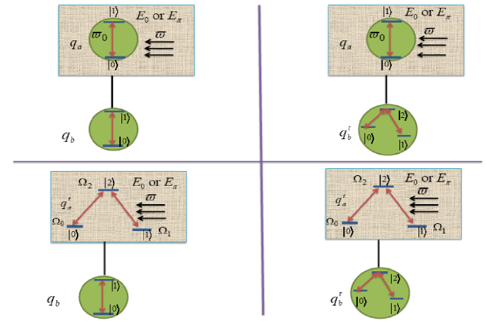
Figure 1: Schematic diagram of the suggested models. (a) A system consists of two qubits one of them is driven by classical external random field with frequency $\omega$. (b) A qubit-qutrit system where the qubit is driven by CERF with frequency $\omega$ and the qutrit is prepared in $\Lambda$ configuration with one upper state $\bigl{|}2\bigr{\rangle}$ with energy $\Omega_{2}$ and two lowers $\bigl{|}0\bigr{\rangle}$ and $\bigl{|}1\bigr{\rangle}$ with energies $\Omega_{0}$ and $\Omega_{1}$, respectively. (c) A qubit-qutrit system, where the qutrit is driven by the CERF with frequency $\omega$ (d) A system consists of two-qutrits prepared in $\Lambda$ configuration defined as (c), where only one qutrit is driven by CERF.

It is assumed that, one of the subsystems of each system interacts locally with its own environment which is described by a single classical random external field (CERF). This field has a frequency $\omega$ and a random phase $\phi$ which equals either $0$ or $\pi$ with probability $P=0.5$. The schematic description is shown in Fig.(1a). In the rotating frame approximations, the Hamiltonian, $\mathcal{H}$ of the single qubit-field system is given by,

$$\mathcal{H}_{q-f}=\frac{\omega_{0}-\omega}{2}\sigma_{z}+i\hbar g(\sigma_{+}e^{-i\phi}-\sigma_{-}e^{i\phi}),$$ (1)

where $g$ is the coupling strength between the qubit and the CREF, $\sigma_{\pm}$ are the raising and lowering operators of the single qubit with frequency $\omega_{0}$. For the suggested 2-qubit systems, it is assumed that,

• Only one qubit is driven by the CERF.

• Only the resonances case is considered i.e., $\omega_{0}=\omega$.

• The interaction between the qubit and its environment is strong enough, where the dissipation between the vacuum and the qubit is forbidden.

By considering the above assumptions, the final state at $t>0$ can be written as,

$$\rho_{2\times 2}(t)=\frac{1}{2}\sum_{j=1}^{2}\left\{e^{-i\mathcal{H}_{j}t}\rho_{2\times 2}(0)e^{i\mathcal{H}_{j}t}\right\},$$ (2)

where $\mathcal{H}_{j}=i\hbar g_{i}(\sigma_{+}e^{-i\phi_{j}}-\sigma_{-}e^{i\phi_{j}})$, j=1,2 with $\phi_{1}=0$ and $\phi_{2}=\pi$, respectively and we set $\hbar=1$ for simplicity. The initial state $\rho_{2\times 2}(0)$ represents the state of a system consists of $2\times 2$ dimensions, i.e., 2-qubits system.

2.2 Dynamics of qubit-qutrit systems

This model represents a $2\times 3$ dimensional system. It is assumed that, only one subsystem is driven by the CERF. However, if the qubit is driven by the classical external random field, then the dynamics of the system is governed by Eq.(2) (see Fig.(1b)). On the other hand, if we allow the $3D$ subsystem, namely the qutrit, to be driven by the local CERF, then the Hamiltonian which describes this system depends on the configuration of the qutrit-system (see Fig.(1c)). Let us consider that, the qutrit is initially prepared in $\Lambda$ configuration [20]. In this case, the Hamiltonian which governs the interaction between the CERF and the single qutrit is given by,

$$\mathcal{H}_{qt-f} = \sum_{\ell=0}^{2}\omega_{\ell}S_{\ell}+g_{1}(e^{-i\phi}S_{12}+e^{i\phi}S_{21})+g_{2}(e^{-i\phi}S_{20}+e^{i\phi}S_{02}),$$ (3)

$$=\mathcal{H}_{0}+\mathcal{H}_{int},$$

where $\omega_{\ell},g_{\ell},\ell=1,2$ are the frequencies of the external fields and the coupling strength between the field and the qutrit. The operators $S_{ij}$, where $(i,j)\in{12,21,20,02}$, obey the $SU(3)$ algebra. For this suggested system, we consider the following assumptions:

• The single qutrit system has one upper level $\bigl{|}2\bigr{\rangle}$ with frequency $\Omega_{2}$ and two lower levels $\bigl{|}0\bigr{\rangle}$ and $\bigl{|}1\bigr{\rangle}$ with frequencies $\Omega_{0}$ and $\Omega_{1}$, respectively.

• The transitions between the $\bigl{|}0\bigr{\rangle}\leftrightarrow\bigl{|}2\bigr{\rangle}$ and $\bigl{|}1\bigr{\rangle}\leftrightarrow\bigl{|}2\bigr{\rangle}$ are dipole allowed, while between $\bigl{|}0\bigr{\rangle}\leftrightarrow\bigl{|}1\bigr{\rangle}$ is dipole forbidden, i.e., there is no interaction.

• The non-degeneracy case is considered [21, 22], namely $(\Omega_{2}-\Omega_{1})-(\Omega_{2}-\Omega_{0})\gg g_{\ell}$, $\ell=1,2$.

• The resonance case is considered i.e. $\Omega_{2}-\Omega_{0}=\omega_{1}$, $\Omega_{2}-\Omega_{1}=\omega_{2}$.

By considering the above assumptions, the dynamics of the qubit-qutrit system is given by,

$$\rho_{2\times 3}(t) = \frac{1}{2}\sum_{i=1}^{2}\left\{e^{-i\mathcal{H}_{int}t}\rho_{2\times 3}(0)e^{i\mathcal{H}_{int}t}\right\},\quad\mbox{with}$$

$$\mathcal{H}_{int} = g_{1}(e^{-i\phi_{i}}S_{12}+e^{i\phi_{i}}S_{21})+g_{2}(e^{-i\phi_{i}}S_{20}+e^{i\phi_{i}}S_{02}),~{}i=0,\pi.$$ (4)

2.3 Dynamics of qutrit-qutrit system

In this case, the initial system consists of two $-$three levels subsystems, namely two qutrits, which represent a generalization of a qubit. The state of the qutrit can be spanned by the three orthogonal basis $\bigl{|}0\bigr{\rangle},\bigl{|}1\bigr{\rangle},\bigl{|}2\bigr{\rangle}$. Physically, qutrit can be represented by three-level atoms [23, 24, 25] (see Fig.(1d)). In this treatment, we consider only one qutrit is driven by the CERF, where both qutrits are initially prepared in $\Lambda$ configuration. Moreover, we consider the same assumptions listed above(qubit-qutrit case). The dynamics of the qutrit-qutrit system $\rho_{3\times 3}(0)$ is given by,

$$\rho_{3\times 3}(t)=\frac{1}{2}\sum_{i=1}^{2}\left\{e^{-i\mathcal{H}_{int}t}\rho_{3\times 3}(0)e^{i\mathcal{H}_{int}t}\right\},$$ (5)

where $\mathcal{H}_{int}$ is given from Eq.(4).

3 Survival Entanglement

In this section, we obtain analytical solutions for all the above systems. The behavior of entanglement between each two subsystems will be discussed, where the amount of entanglement is quantified by using a measure called negativity. This measure is an acceptable measure for any bipartite system of any dimension [26]. For a state $\rho_{12}$, with dimensions $d_{1}\times d_{2}$ where $d_{1}<d_{2}$, the negativity, $\mathcal{N}$ is defined as,

$$\mathcal{N}=\frac{1}{d_{1}-1}\left\{||\rho_{12}^{T_{2}}||-1\right\},$$ (6)

where $\rho_{12}^{T_{2}}$ is the partial transpose with respect to the largest party (second-partite) and $||.||$ is the trace norm [26, 27]

3.1 Qubit-qubit systems

Let us assume that, the two qubits state is given by $X$-state, which can be described by the computational basis $"0"$ and $"1"$ as,

$$\rho_{x}(0) = \frac{1+c_{33}}{2}\Bigl{(}\bigl{|}00\bigr{\rangle}\bigl{\langle}00\bigr{|}+\bigl{|}11\bigr{\rangle}\bigl{\langle}11\bigr{|}\Bigr{)}+\frac{1-c_{33}}{2}\Bigl{(}\bigl{|}01\bigr{\rangle}\bigl{\langle}01\bigr{|}+\bigl{|}10\bigr{\rangle}\bigl{\langle}10\bigr{|}\Bigr{)}$$ (7)

$$+\frac{c_{11}+c_{22}}{2}\Bigl{(}\bigl{|}01\bigr{\rangle}\bigl{\langle}10\bigr{|}+\bigl{|}10\bigr{\rangle}\bigl{\langle}01\bigr{|}\Bigr{)}+\frac{c_{11}-c_{22}}{2}\Bigl{(}\bigl{|}00\bigr{\rangle}\bigl{\langle}11\bigr{|}+\bigl{|}11\bigr{\rangle}\bigl{\langle}00\bigr{|}\Bigr{)},$$

where $c_{ij}=tr\{\rho_{x}(0)\sigma_{i}\sigma_{j}\},i,j=1,2,3$ and $\sigma_{i,j}$ are the Pauli matrices for the first and the second qubits, respectively. From this state, one can obtain a maximum entangled classes of states by setting $c_{ij}=\pm 1$, Werner state by setting $c_{ij}=x$ and a generalized Werner state for $c_{11}=x_{1},c_{22}=x_{2}$ and $c_{33}=x_{3}$.

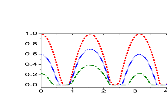
Figure 2: The evolution of the entanglement for two dimensional system (two-qubits) against $\tau$. The dash, dot and dash-dot curves for MES,( $c_{11}=c_{22}=c_{33}=-1$), Werner state with $x=-0.8$ and a generalized Werner state ( $c_{11}=-0.8,c_{22}=-0.7$, and $c_{33}=-0.6$), respectively .

If only one qubit is driven by the classical external random field, then the final state of the system at a time $\tau>0$ is given by,

$$\rho_{x}(t) = \mathcal{R}_{1}\bigl{|}00\bigr{\rangle}\bigl{\langle}00\bigr{|}+\mathcal{R}_{2}\bigl{|}00\bigr{\rangle}\bigl{\langle}10\bigr{|}+\mathcal{R}_{3}\bigl{|}00\bigr{\rangle}\bigl{\langle}11\bigr{|}+\mathcal{R}_{4}\bigl{|}01\bigr{\rangle}\bigl{\langle}01\bigr{|}+\mathcal{R}_{5}\bigl{|}01\bigr{\rangle}\bigl{\langle}10\bigr{|}+\mathcal{R}_{6}\bigl{|}10\bigr{\rangle}\bigl{\langle}01\bigr{|}$$ (8)

$$+\mathcal{R}_{7}\bigl{|}10\bigr{\rangle}\bigl{\langle}10\bigr{|}+\mathcal{R}_{8}\bigl{|}10\bigr{\rangle}\bigl{\langle}11\bigr{|}+\mathcal{R}_{9}\bigl{|}11\bigr{\rangle}\bigl{\langle}00\bigr{|}+\mathcal{R}_{10}\bigl{|}11\bigr{\rangle}\bigl{\langle}10\bigr{|}+\mathcal{R}_{11}\bigl{|}11\bigr{\rangle}\bigl{\langle}11\bigr{|},$$

where,

$$\mathcal{R}_{1} = \frac{1+c_{33}}{2}cos^{2}(\tau)+\frac{1-c_{33}}{2}sin^{2}(\tau),$$

$$\mathcal{R}_{2} = -\frac{1+c_{33}}{2}\sin(\tau)\cos(\tau),$$

$$\mathcal{R}_{3} = \frac{c_{11}-c_{22}}{2}cos^{2}(\tau)-\frac{c_{11}+c_{22}}{2}sin^{2}(\tau),$$

$$\mathcal{R}_{4} = \frac{1-c_{33}}{2}cos^{2}(\tau)+\frac{1+c_{33}}{2}sin^{2}(\tau),$$

$$\mathcal{R}_{5} = \frac{c_{11}+c_{22}}{2}cos^{2}(\tau)-\frac{c_{11}-c_{22}}{2}sin^{2}(\tau)=\mathcal{R}_{6},$$

$$\mathcal{R}_{7} = \frac{1-c_{33}}{2}cos^{2}(\tau)-\frac{1+c_{33}}{2}sin^{2}(\tau)$$

$$\mathcal{R}_{8} = -\frac{c_{11}+c_{22}}{4}\sin(2\tau),\quad\mathcal{R}_{9}=\mathcal{R}_{3},$$

$$\quad\mathcal{R}_{10} = -\frac{c_{11}-c_{22}}{4}\sin(2\tau),\quad\mathcal{R}_{11}=\mathcal{R}_{1}.$$ (9)

where $gt=\tau$

In Fig.(2), we investigate the effect of the classical external random field on three different classes of two-qubit systems: maximum entangled class (MES), where we set $c_{11}=c_{22}=c_{33}=-1$, Werner state, with $(c_{11}=c_{22}=c_{33}=x=-0.8)$ and partially entangled classes (PES) with $c_{11}=-0.8,c_{22}=-0.7,c_{33}=-0.6$. The general behavior shows that, the entanglement decays as the time increases for all these initial states. The phenomena of sudden death of entanglement is depicted for each MES and PES. However, the time death increases for initially less entangled states. For lager interaction time, the entanglement re-birth again to reach its maximum bounds which depend on the entanglement of the initial states. For partially entangled states, the upper bounds of entanglement are larger than the initial entanglement in some intervals of time. Moreover, the upper bounds are reached at the same time for all states.

3.2 Qubit-Qutrit systems

In this subsection,a system consisting of two different dimensional subsystems is considered: one is a qubit (2D) and the other is a qutrit (3D). Analytical solutions for the final states are obtained for different families. The first state is known by one parameter family [27] and the second known by a two parameters family [30]. The time evolution is obtained when only one of their subsystems is driven by classical external random field.

3.2.1 One parameter family

This state represents a qubit-qutrit system which is defined by $2\times 3$ dimensions. It is described by one parameter as,

$$\rho_{1p}(0) = \frac{\mathcal{P}}{2}\bigl{(}\bigl{|}00\bigr{\rangle}\bigl{\langle}00\bigr{|}+\bigl{|}01\bigr{\rangle}\bigl{\langle}01\bigr{|}+\bigl{|}11\bigr{\rangle}\bigl{\langle}11\bigr{|}\bigr{)}+\frac{\mathcal{P}}{2}\bigl{(}\bigl{|}12\bigr{\rangle}\bigl{\langle}12\bigr{|}+\bigl{|}12\bigr{\rangle}\bigl{\langle}00\bigr{|}+\bigl{|}00\bigr{\rangle}\bigl{\langle}12\bigr{|}\bigr{)}.$$ (10)

$$+\frac{1-2\mathcal{P}}{2}\left(\bigl{|}02\bigr{\rangle}\bigl{\langle}02\bigr{|}+\bigl{|}10\bigr{\rangle}\bigl{\langle}02\bigr{|}+\bigl{|}10\bigr{\rangle}\bigl{\langle}10\bigr{|}+\bigl{|}02\bigr{\rangle}\bigl{\langle}10\bigr{|}\right)$$

This state has quantum correlation for $\mathcal{P}\in[0,\frac{1}{3})\bigcup(\frac{1}{3},0.5]$, i.e., it is disentangled at $\mathcal{P}=\frac{1}{3}$ only. Now we consider the following two cases:

• Only the qubit is driven by the CERF
  The time evolution of the initial state (10) can be obtained by using Eq.(2). For $\tau>0$, the final state $\rho_{1p}(t)$ can be written explicitly as,

  $$\rho_{1p}^{q_{b}}(t) = \mathcal{L}_{1}^{q_{b}}\bigl{|}00\bigr{\rangle}\bigl{\langle}00\bigr{|}+\mathcal{L}_{2}^{q_{b}}\bigl{|}00\bigr{\rangle}\bigl{\langle}12\bigr{|}+\mathcal{L}_{3}^{q_{b}}\bigl{|}01\bigr{\rangle}\bigl{\langle}01\bigr{|}+\mathcal{L}_{4}^{q_{b}}\bigl{|}02\bigr{\rangle}\bigl{\langle}02\bigr{|}+\mathcal{L}_{5}^{q_{b}}\bigl{|}10\bigr{\rangle}\bigl{\langle}10\bigr{|}$$

  $$+\mathcal{L}_{6}^{q_{b}}\bigl{|}10\bigr{\rangle}\bigl{\langle}02\bigr{|}+\mathcal{L}_{7}^{q_{b}}\bigl{|}02\bigr{\rangle}\bigl{\langle}10\bigr{|}+\mathcal{L}_{8}^{q_{b}}\bigl{|}11\bigr{\rangle}\bigl{\langle}11\bigr{|}+\mathcal{L}_{9}^{q_{b}}\bigl{|}12\bigr{\rangle}\bigl{\langle}12\bigr{|}+\mathcal{L}_{10}^{q_{b}}\bigl{|}12\bigr{\rangle}\bigl{\langle}00\bigr{|},$$

  where, the superscript $q_{b}$ refers to the qubit while the subscript $1p$ means one parameter family. The coefficients $\mathcal{L}^{q_{b}}_{j},j=1...10$ are given by,

  $$\mathcal{L}_{1,2}^{q_{b}} = \frac{\mathcal{P}}{2}\cos^{2}(\tau)\pm\frac{1-2\mathcal{P}}{2}\sin^{2}(\tau),\quad\mathcal{L}_{3}^{q_{b}}=\frac{\mathcal{P}}{2},$$

  $$\mathcal{L}_{4}^{q_{b}} = \mathcal{L}_{5}^{q_{b}}=\frac{\mathcal{P}}{2}\sin^{2}(\tau)+\frac{1-2\mathcal{P}}{2}\cos^{2}(\tau),$$

  $$\mathcal{L}_{6}^{q_{b}} = \mathcal{L}_{7}^{q_{u}}=\frac{1-2\mathcal{P}}{2}\cos^{2}(\tau)-\frac{\mathcal{P}}{2}\sin^{2}(\tau),$$

  $$\mathcal{L}_{8}^{q_{b}} = \mathcal{L}_{3}^{q_{b}},\quad\mathcal{L}_{9}^{q_{b}}=\mathcal{L}_{1}^{q_{b}},\quad\mathcal{L}_{10}^{q_{b}}=\mathcal{L}_{1}^{q_{b}},\mbox{where}~{}\quad gt=\tau.$$ (12)

• Only the qutrit is driven by CERF
  In this case, it is assumed that only the qutrit is allowed to be driven by the classical external random field, where the non-degenerate state is considered [21, 22]. The final state is given by,

  $$\rho_{1p}^{q_{t}} = \mathcal{L}_{1}^{q_{t}}\bigl{|}00\bigr{\rangle}\bigl{\langle}00\bigr{|}+\mathcal{L}_{2}^{q_{t}}\bigl{|}00\bigr{\rangle}\bigl{\langle}02\bigr{|}+\mathcal{L}_{3}^{q_{t}}\bigl{|}00\bigr{\rangle}\bigl{\langle}10\bigr{|}+\mathcal{L}_{4}^{q_{t}}\bigl{|}00\bigr{\rangle}\bigl{\langle}12\bigr{|}+\mathcal{L}_{5}^{q_{t}}\bigl{|}01\bigr{\rangle}\bigl{\langle}00\bigr{|}$$

  $$+\mathcal{L}_{6}^{q_{t}}\bigl{|}01\bigr{\rangle}\bigl{\langle}01\bigr{|}+\mathcal{L}_{7}^{q_{t}}\bigl{|}01\bigr{\rangle}\bigl{\langle}10\bigr{|}+\mathcal{L}_{8}^{q_{t}}\bigl{|}01\bigr{\rangle}\bigl{\langle}11\bigr{|}+\mathcal{L}_{9}^{q_{u}}\bigl{|}02\bigr{\rangle}\bigl{\langle}00\bigr{|}+\mathcal{L}_{10}^{q_{t}}\bigl{|}02\bigr{\rangle}\bigl{\langle}02\bigr{|}$$

  $$+\mathcal{L}_{11}^{q_{t}}\bigl{|}10\bigr{\rangle}\bigl{\langle}00\bigr{|}+\mathcal{L}_{12}^{q_{t}}\bigl{|}10\bigr{\rangle}\bigl{\langle}02\bigr{|}+\mathcal{L}_{13}^{q_{t}}\bigl{|}10\bigr{\rangle}\bigl{\langle}10\bigr{|}+\mathcal{L}_{14}^{q_{t}}\bigl{|}10\bigr{\rangle}\bigl{\langle}11\bigr{|}+\mathcal{L}_{15}^{q_{t}}\bigl{|}10\bigr{\rangle}\bigl{\langle}12\bigr{|}$$

  $$+\mathcal{L}_{16}^{q_{t}}\bigl{|}11\bigr{\rangle}\bigl{\langle}00\bigr{|}+\mathcal{L}_{17}^{q_{t}}\bigl{|}11\bigr{\rangle}\bigl{\langle}11\bigr{|}+\mathcal{L}_{18}^{q_{t}}\bigl{|}11\bigr{\rangle}\bigl{\langle}10\bigr{|}+\mathcal{L}_{19}^{q_{t}}\bigl{|}12\bigr{\rangle}\bigl{\langle}10\bigr{|}+\mathcal{L}_{20}^{q_{t}}\bigl{|}12\bigr{\rangle}\bigl{\langle}12\bigr{|}$$

  $$+\mathcal{L}_{21}^{q_{t}}\bigl{|}00\bigr{\rangle}\bigl{\langle}11\bigr{|}+\mathcal{L}_{22}^{q_{t}}\bigl{|}02\bigr{\rangle}\bigl{\langle}10\bigr{|}+\mathcal{L}_{23}^{q_{t}}\bigl{|}10\bigr{\rangle}\bigl{\langle}01\bigr{|}+\mathcal{L}_{24}^{q_{t}}\bigl{|}11\bigr{\rangle}\bigl{\langle}01\bigr{|}+\mathcal{L}_{25}^{q_{t}}\bigl{|}12\bigr{\rangle}\bigl{\langle}00\bigr{|}$$

  where, the subscript $q_{t}$ refers the qutrit The coefficients $\mathcal{L}_{j}^{q_{t}},j=1...25$ are given by,

  $$\mathcal{L}_{1}^{q_{t}} = \frac{\mathcal{P}}{2}\cos^{2}(\tau_{1})+\frac{1-2\mathcal{P}}{2}\sin^{2}(\tau_{1}),\quad\mathcal{L}_{2}^{q_{t}}=-\frac{1-2\mathcal{P}}{4}\sin(\tau_{1})\sin(2\tau_{2}),$$

  $$\mathcal{L}_{3}^{q_{t}} = -\frac{1-\mathcal{P}}{4}\sin(2\tau_{1})\sin(\tau_{2}),\quad\mathcal{L}_{4}=\frac{\mathcal{P}}{2}\cos(\tau_{1})\cos(\tau_{2}),\quad$$

  $$\mathcal{L}_{5}^{q_{t}} = \frac{1-2\mathcal{P}}{8}\sin(2\tau_{1})\sin(2\tau_{2}),$$

  $$\mathcal{L}_{6}^{q_{t}} = \frac{\mathcal{P}}{2}\Bigl{(}\sin^{2}(\tau_{1})+\cos^{2}(\tau_{2})\cos^{2}(\tau_{2})\Bigr{)}+\frac{1-2\mathcal{P}}{2}\cos^{2}(\tau_{1})\sin^{2}(\tau_{2}),$$

  $$\mathcal{L}_{7}^{q_{t}} = \frac{\mathcal{P}}{2}\sin^{2}(\tau_{1})\cos(\tau_{2}),\quad\mathcal{L}_{8}^{q_{t}}=\frac{1-\mathcal{P}}{4}\sin(2\tau_{1})\sin(\tau_{2}),\quad$$

  $$\mathcal{L}_{9}^{q_{t}} = -\frac{1-2\mathcal{P}}{4}\sin(\tau_{1})\sin(2\tau_{2}),$$

  $$\mathcal{L}_{10}^{q_{t}} = \frac{\mathcal{P}}{2}\sin^{2}(\tau_{2})+\frac{1-2\mathcal{P}}{2}\cos^{2}(\tau_{2}),\quad\mathcal{L}_{11}^{q_{t}}=\frac{\mathcal{P}}{2}\sin(\tau_{1})\sin(\tau_{2})\Bigl{(}\cos(\tau_{1})+\cos(\tau_{2})\Bigr{)},$$

  $$\mathcal{L}_{12}^{q_{t}} = \frac{1-2\mathcal{P}}{2}\cos(\tau_{1})\cos(\tau_{2}),\quad\mathcal{L}_{13}^{q_{t}}=\frac{\mathcal{P}}{2}\sin^{2}(\tau_{1})+\frac{1-2\mathcal{P}}{2}\cos^{2}(\tau_{2}),$$

  $$\mathcal{L}_{14}^{q_{t}} = \frac{\mathcal{P}}{8}\sin(2\tau_{1})\sin(2\tau_{2}),\quad\mathcal{L}_{15}^{q_{t}}=-\frac{\mathcal{P}}{4}\sin(2\tau_{1})\cos(\tau_{2}),\quad$$

  $$\mathcal{L}_{16}^{q_{t}} = \frac{1-2\mathcal{P}}{2}\sin^{2}(\tau_{1})\cos(\tau_{2}),$$

  $$\mathcal{L}_{17}^{q_{t}} = \frac{\mathcal{P}}{2}\cos^{2}(\tau_{1})+\frac{1-2\mathcal{P}}{2}\sin^{2}(\tau_{2}),\quad\mathcal{L}_{18}^{q_{t}}=\mathcal{L}_{14}^{q_{t}},\quad\mathcal{L}_{19}^{q_{t}}=\mathcal{L}_{15}^{q_{u}},\quad\mathcal{L}_{20}^{q_{t}}=\frac{\mathcal{P}}{2},$$

  $$\mathcal{L}_{21}^{q_{t}} = \mathcal{L}_{16}^{q_{t}},\quad\mathcal{L}_{22}^{q_{t}}=\mathcal{L}_{12}^{q_{t}},\quad\mathcal{L}_{23}^{q_{t}}=\mathcal{L}_{7}^{q_{t}},\quad\mathcal{L}_{24}^{q_{t}}=\frac{\mathcal{P}}{4}\sin(\tau_{1})\sin(\tau_{2}),\quad\mathcal{L}_{25}^{q_{t}}=\mathcal{L}_{4}^{q_{t}}.$$ (14)

  where $g_{1}t=\tau_{1}$ and $g_{2}t=\tau_{2}$.

  

  Figure 3: Entanglement of one parameter family qubit-qutrit system, where the dash and dash-dot curves stand for $p=0$ (MES) and $p=0.5$ (PES). (a) qubit is driven (b) qutrit is driven, where we set $\tau_{1}=\tau_{2}=\tau^{\prime}$

  The behavior of entanglement for a system is prepared initially in a qubit-qutrit state of one parameter family type is depicted in Fig.(3), where it is assumed that only the qubit or the qutrit are driven by the classical external random field. Two values of the parameter $\mathcal{P}$ are considered, $\mathcal{P}=0$ for a system is initially prepared in a maximum entangled state [28] and $\mathcal{P}=0.5$ for a system is initially prepared in a partially entangled state (PES).

  Fig.(3a), describes the entanglement behavior between the two subsystems (qubit and qutrit) when only the qubit is driven by the CERF. The general behavior shows that, at $\tau=0$, the entanglement between the two subsystems is maximum, ($\mathcal{N}=1)$. However, as soon as the interaction is switched on between the qubit and the CERF, the entanglement decays fast to reach its minimum bound $(\mathcal{N}=0.0292)$ for the first time at $\tau=0.8$. As $\tau$ increases further, the entanglement increases suddenly to reach its maximum value $(\mathcal{N}=1)$ for the first time at $\tau=1.6$. For larger values of $\tau$, the behavior of entanglement is repeated periodically, where the entanglement between the two subsystems never vanishes. On the other hand, if we start from a partially entangled state ($\mathcal{P}=0.5$), the behavior of entanglement is similar to that predicted for MES. However, the lower bounds of entanglement are larger than those depicted for the two qubit system (MES), while the death time is smaller.

  Fig.(3b) shows the dynamics of entanglement when only the qutrit is driven by the CERF, where the same initial state settings are considered, ($\mathcal{P}=0$ and $0.5$). The general behavior shows that, the entanglement decreases as soon as the interaction is switched on. The decay rate is much smaller than that shown in Fig.(3a), where only the qubit is driven by the CERF. It is clear that, the entanglement decays slowly and the phenomena of the sudden changes of entanglement appear clearly [29]. The decay time is much larger than that depicted in Fig.(3a), where the two subsystems are completely separable for the first time at $\tau\simeq 1.5$.

3.2.2 Two parameters Family

In computational basis, the state which describes this family can be written as [30],

$$\rho_{2p}(0) = \alpha(\bigl{|}02\bigr{\rangle}\bigl{\langle}02\bigr{|}+\bigl{|}12\bigr{\rangle}\bigl{\langle}12\bigr{|})+\beta(\bigl{|}00\bigr{\rangle}\bigl{\langle}00\bigr{|}+\bigl{|}11\bigr{\rangle}\bigl{\langle}11\bigr{|})+\frac{\beta+\gamma}{2}(\bigl{|}01\bigr{\rangle}\bigl{\langle}01\bigr{|}+\bigl{|}10\bigr{\rangle}\bigl{\langle}10\bigr{|})$$ (15)

$$+\frac{\beta-\gamma}{2}(\bigl{|}01\bigr{\rangle}\bigl{\langle}10\bigr{|}+\bigl{|}10\bigr{\rangle}\bigl{\langle}01\bigr{|}),$$

where $\gamma+2\alpha+3\beta=1$. The two parameters family state (15) is entangled for $\beta=0$, $\alpha\in[0,\frac{1}{2}]$ and $\gamma\in[\frac{1}{2},1]$. Moreover, if we set $\alpha=\frac{1}{2}$ and $\gamma=1$, then the state (15) turns into a maximum entangled state (MES). Now, let us consider the following two cases:

• Only the qubit is driven by the CERF
  In this case, the time evolution of the initial state (15) is given by the following density operator,

  $$\rho_{2p}(t) = \mathcal{M}_{1}\bigl{|}00\bigr{\rangle}\bigl{\langle}00\bigr{|}+\mathcal{M}_{2}\bigl{|}01\bigr{\rangle}\bigl{\langle}01\bigr{|}+\mathcal{M}_{3}\bigl{|}10\bigr{\rangle}\bigl{\langle}10\bigr{|}+\mathcal{M}_{4}\bigl{|}01\bigr{\rangle}\bigl{\langle}10\bigr{|}+\mathcal{M}_{5}\bigl{|}10\bigr{\rangle}\bigl{\langle}01\bigr{|}$$

  $$+ \mathcal{M}_{6}\bigl{|}11\bigr{\rangle}\bigl{\langle}11\bigr{|}+\mathcal{M}_{7}\bigl{|}00\bigr{\rangle}\bigl{\langle}11\bigr{|}+\mathcal{M}_{8}\bigl{|}11\bigr{\rangle}\bigl{\langle}00\bigr{|}+\mathcal{M}_{9}\bigl{|}02\bigr{\rangle}\bigl{\langle}02\bigr{|}+\mathcal{M}_{10}\bigl{|}12\bigr{\rangle}\bigl{\langle}12\bigr{|},$$

  where,

  $$\mathcal{M}_{1} = \beta\cos^{2}(\tau)+\frac{\beta+\gamma}{2}\sin^{2}(gt),\mathcal{M}_{2}=\beta\sin^{2}(\tau)+\frac{\beta+\gamma}{2}\cos^{2}(\tau)$$

  $$\mathcal{M}_{3} = \mathcal{M}_{2},\quad\mathcal{M}_{4}=\mathcal{M}_{5}=\frac{\beta-\gamma}{2}\cos^{2}(\tau),\quad\mathcal{M}_{6}=\mathcal{M}_{1},$$

  $$\mathcal{M}_{7} = \mathcal{M}_{8}=-\frac{\beta-\gamma}{2}\sin^{2}(\tau),\quad\mathcal{M}_{9}=\mathcal{M}_{10}=\alpha.$$ (17)

  

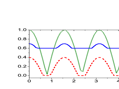
  Figure 4: Entanglement of the two parameters family qubit-qutrit system (a) when only the qubit is driven by CERF and (b) Only the qutrit is driven by the CERF, where $\tau_{1}=\tau_{2}=\tau^{\prime}$. The dot curve for MES with $(\beta=0,\gamma=1,\alpha=0.5)$, while the dash and the solid curves for PES with $(\beta=0.2,\gamma=0.7)$, and $(\beta=0.2,\gamma=0.6)$, respectively.

• Only the qutrit is driven by the CERF

In this case, the final state of the system is described by a matrix of $6$ dimensions, where the non-zero elements are given by,

$$\varrho_{00,00} = \beta c_{1}^{2}+\alpha s_{1}^{2},\quad\varrho_{00,01}=\varrho_{01,00}=\frac{\alpha}{4}s_{1}s_{2},\quad\varrho_{00,02}=-\frac{\alpha}{2}s_{1}\sin(2\tau_{2}),$$

$$\varrho_{01,01} = \beta s_{1}^{2}+c_{1}^{2}\left(\alpha s_{2}^{2}+\frac{\beta+\gamma}{2}c_{2}^{2}\right),\quad\varrho_{01,10}=\varrho_{10,01}=\frac{\beta-\gamma}{2}c_{1}^{2}c_{2},$$

$$\varrho_{02,00} = \varrho_{0,02},\quad\varrho_{02,02}=\alpha c_{2}^{2}+\frac{\beta+\gamma}{2}s_{2}^{2},\quad\varrho_{02,10}=\frac{\beta-\gamma}{2}s_{1}s_{2}$$

$$\varrho_{10,10} = \alpha s_{1}^{2}+\frac{\beta+\gamma}{2}c_{1}^{2},\quad\varrho_{10,11}=\frac{\alpha}{4}\sin(2\tau_{1})\sin(\tau_{2}),\quad\varrho_{10,12}=-\frac{\alpha}{2}s_{1}\sin(2\tau_{2})$$

$$\varrho_{11,02} = \varrho_{02,10},\quad\varrho_{11,10}=\varrho_{10,11},\quad\varrho_{12,10}=\varrho_{10,12},\quad\varrho_{11,02}=\alpha c_{2}^{2}+s_{2}^{2}\beta,$$ (18)

with $s_{i}=\sin(\tau_{i}),c_{i}=\cos(\tau_{i}),\tau_{i}=g_{i}t,~{}i=1,2$

In Fig.(4), the amount of survival entanglement between the two subsystems (qubit and qutrit) is displayed for different initial state settings. The behavior of entanglement when only the qubit is driven by the classical external random field is depicted in Fig.(4a). If the initial system is initially prepared in a maximum entangled state, then the entanglement suddenly decays to reach its minimum value for the first time at $\tau\simeq 0.8$, then suddenly increases to be maximum $(\mathcal{N}=1)$. This behavior is periodically repeated as $\tau$ increases. The phenomenon of long-lived entanglement is predicted for systems that are initially prepared in partially entangled states, while the phenomena of sudden decay and death of entanglement are shown for systems that are initially prepared with small entanglement.

Fig.(4b), shows the behavior of entanglement when only the qutrit is driven by CERF. In this case, for initially MES, the entanglement decays very fast to death completely at $\tau^{\prime}\simeq 0.7$. For this class of states, the phenomenon of sudden birth of entanglement is depicted, where the death time is much larger than that shown for one parameter family. For initially less entangled state, the entanglement decreases then increases gradually. The phenomenon of entanglement death can be seen only for a short time for systems which have small initial entanglement.

From this figure, one concludes that, systems which are initially prepared in MES are more sensitive to the classical external random field than those which are prepared in PES. If the larger dimensional systems are driven by the CERF, then the entanglement of the MES are liable to sudden death for a longer time. Systems which are initially prepared in PES are more robust than those prepared in MES for the CERF. The long-lived entanglement can be observed if one has the ability to control the parameters which describe the initial state. Consequently, one can perform quantum information tasks even in the presences of these types of noises.

3.3 Qutrit-qutrit system

A system of qutrit-qutrit can be defined by,

$$\rho_{qt}(0) = \bigl{|}\psi_{qt}(0)\bigr{\rangle}\bigl{\langle}\psi_{qt}(0)\bigr{|},\quad\mbox{where}$$ (19)

$$\bigl{|}\psi_{qt}(0)\bigr{\rangle}=a_{1}\bigl{|}00\bigr{\rangle}+a_{2}\bigl{|}11\bigr{\rangle}+a_{3}\bigl{|}22\bigr{\rangle},\quad$$

where $a_{i},i=1,2,3$ are real and $a_{1}^{2}+a_{2}^{2}+a_{3}^{2}=1$. In this treatment, it is assumed that both qutrits are prepared in $\Lambda$ configuration and only the first qutrit is driven by the classical external random field CERF. By using Eq.(5), one gets the final state of the qutrit-qutrit system at any value of $\tau_{1}=\tau_{2}>0$. This final state is defined by a $9\times 9$ matrix, where the non-zero elements are given by,

$$\rho_{00,00} = a_{1}^{2}c_{1}^{2},\quad\rho_{00,11}=a_{1}a_{2}c_{1}^{2}c_{2},\quad\rho_{00,22}=a_{1}a_{3}c_{1}c_{2},\quad\rho_{00,02}=-a_{1}a_{3}c_{1}s_{1}s_{2},$$

$$\rho_{11,00} = a_{1}a_{2}c_{1}^{2}c_{2},\quad\rho_{11,11}=a_{2}^{2}c_{1}^{2}c_{2}^{2},\quad\rho_{11,22}=a_{2}a_{3}c_{1}c_{2}^{2},\quad\rho_{00,02}=-a_{2}a_{3}c_{1}c_{2}s_{1}s_{2},$$

$$\rho_{22,00} = a_{3}a_{1}c_{1}c_{2},\quad\rho_{22,11}=a_{2}a_{3}c_{1}c_{2}^{2},\quad\rho_{22,22}=a_{3}^{2}c_{2}^{2},\quad\rho_{22,02}=-a_{3}^{2}c_{2}s_{1}s_{2},$$

$$\rho_{02,00} = -a_{3}a_{1}s_{1}s_{2}c_{1},\quad\rho_{02,11}=-a_{3}a_{2}s_{1}s_{2}c_{1}c_{2},\quad\rho_{02,22}=-a_{3}^{2}s_{1}s_{2}c_{2},\quad\rho_{02,02}=a_{3}^{2}s_{1}^{2}s_{2}^{2}$$

$$\rho_{21,10} = a_{2}a_{1}s_{1}s_{2},\quad\rho_{21,21}=a_{2}^{2}s_{2}^{2},\quad\rho_{21,12}=a_{2}a_{3}s_{1}s_{2}c_{1},\quad\rho_{21,02}=a_{2}a_{3}s_{1}^{2}s_{2}c_{2},\quad$$

$$\rho_{12,10} = a_{3}a_{1}c_{1}s_{1}s_{2},\quad\rho_{12,21}=a_{2}a_{3}c_{1}s_{2}^{2},\quad\rho_{12,12}=a_{3}^{2}c_{1}^{2}s_{2}^{2},\quad\rho_{12,02}=a_{3}^{2}c_{1}c_{2}s_{1}s_{2},$$

$$\rho_{10,10} = a_{1}^{2}s_{1}^{2},\quad\rho_{10,21}=a_{1}a_{2}c_{1}s_{2},\quad\rho_{10,12}=a_{1}a_{3}^{2}s_{1}c_{1}s_{2},\quad\rho_{10,02}=a_{1}a_{3}s_{1}^{2}c_{2},\quad$$

$$\rho_{02,10} = a_{3}a_{1}s_{1}^{2}c_{2},\rho_{02,21}=a_{3}a_{2}s_{1}s_{2}c_{2},\quad\rho_{02,12}=a_{3}^{2}s_{1}c_{1}s_{2}c_{2},\quad\rho_{02,02}=a_{3}^{2}s_{1}^{2}c_{2}^{2}.$$ (20)

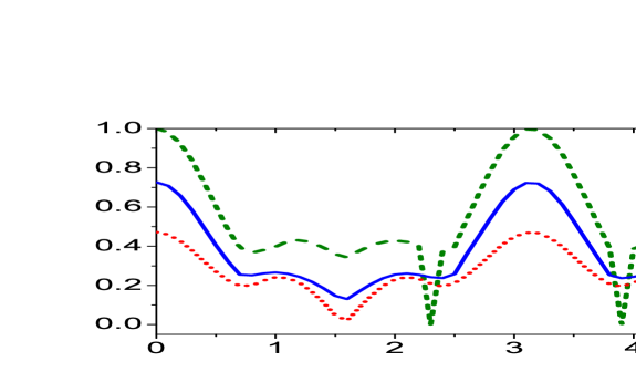
Figure 5: Entanglement of two qutrits-system. The dash curve for MES $(a_{1}=a_{2}=a_{3}=\frac{1}{\sqrt{3}}$) the dot for $(a_{1}=0,a_{2}=\frac{1}{\sqrt{3}},a_{3}=\sqrt{\frac{2}{3}})$ and solid curves for $(a_{1}=0.3,a_{2}=0.4)$, respectively.

In Fig.(5), we plot the behavior of the entanglement when the first qutrit is driven by the CERF. Let us consider that, the system is initially prepared in MES, i.e, we set $a_{i}=\frac{1}{\sqrt{3}},i=1,2,3$. In this case, the general behavior shows that, the entanglement is maximum at $\tau^{\prime}=0$ (before the interaction is switched on). As soon as the interaction between the first qutrit and the classical external random field is switch on, the entanglement decays as the interaction time is increased. However, the entanglement vanishes for the first time at $\tau^{\prime}\simeq 2.4$. For larger time, the entanglement re-increases gradually to reach its maximum value ($\mathcal{N}=1)$ for the first time at $\tau^{\prime}\simeq 3$. This behavior is repeated while increasing the interaction time between the qutrit and CERF.

The effect of CERF on qutrit-qutrit system ( initially prepared in PES) is described also in Fig.(5), where two classes are considered: the first one is obtained by setting $a_{1}=0.3,a_{2}=0.4$, while the second is obtained by setting $a_{1}=0,a_{2}=1/\sqrt{3}$. However, the phenomenon of entanglement sudden changes is depicted for the two cases. For less initial entangled system, the lower bounds of entanglement are larger than those which start with larger degree of entanglement. Moreover, the upper bounds of entanglement are reached at the same time.

From the behavior of negativity, one can conclude that: as soon as the interaction is switched on, the phenomenon of sudden decay of entanglement is depicted for MES and PES. The entanglement suddenly increases to reach their maximum bounds which are dependent on the initial entanglement. However, the upper and lower bounds of entanglement are reached at the same time for all considered states.

4 Conclusion

In this paper, the entanglement of three types of different dimensional systems are discussed. It is assumed that only one subsystem is driven by an external random field. The suggested systems are: qubit-qubit, qubit-qutrit and qutrit qutrit systems, which are described by $2\times 2,~{}2\times 3$ and $3\times 3$ dimensions, respectively. The general behavior shows that, the entanglement is very sensitive to the classical external random field. However, this sensitivity depends on the size of the driven subsystem and the initial degree of entanglement of the system.

Maximum entangled states are the most sensitive states for the external field, where the phenomena of the sudden decay of entanglement, changes, death and sudden re-birth are displayed clearly. On the other hand, partially entangled states, are found more robust than the maximum entangled states to this classical external random field.

The dimensions of the driven subsystems by the external field play an important role on the behavior of entanglement. This result can be observed clearly for the qubit-qutrit systems, where if only the qubit is driven, then the sudden changes of entanglement ( death or birth) are faster than that shown for the case in which only the qutrit is driven by this external field. For the two parameters class, one can observe the phenomenon of long-lived entanglement if the qubit is driven by the external field. However, for one parameter family, partially entangled states are more robust than the two parameters class if the qutrit is driven by the classical external random field.

For qutrit-qutrit system, the entanglement is more robust to the classical external random field than that displayed for qubit-qutrit systems, where the entanglement decays smoothly whereas only the MES lose their entanglement for a very short period of time and the re-birth occurs again shortly. The effect of the dimensions of the driven subsystems by the CERF can be observed by comparing the behavior of survival entanglement between the qubit-qubit and the qutrit-qutrit systems. It is clear that, the entanglement of larger dimensional systems are more robust than smaller systems.

From previous discussions one can conclude that: (i) maximum entangled states are very sensitive to the classical external random field; (ii) the entanglement and hence the information are lost fast for smaller dimensional systems; (iii) one parameter family is more powerful than the two parameters family, where the possibility of losing its correlation is much smaller than that shown for the two parameters family, and consequently their efficiency to perform quantum information tasks is better; (iv) the long-lived entanglement can be depicted for systems are initially prepared in the two parameter family’s class; (v) the two-qutrit system is more robust than the two-qubit system for the classical external random field. Therefore we can induce, that in the context of quantum information and communication, the 2-qutrit systems are much better than the 2-qubit system in the presence of classical external random field.

Acknowledgement: We would like to thank the referee for his/her comments which improve the manuscript.

References

• [1] M. Ban, S. Kitajima and F. Shibata, ” Decoherence of entanglement in the Bloch channel” J. Phys. A 38, 4235 (2005); M. Ban, S. Kitajima and F. Shibata,” Decoherence of quantum information in the non-Markovian qubit channel” J. Phys. A 38, 7161 (2005).
• [2] T. Yu, J. Eberly: Opt. Commu ”Sudden Death of Entanglement: Classical Noise Effects” 264, 393 (2006).
• [3] N. Metwally,”Abrupt decay of entanglement and quantum communication through noise channels”, Quantum Inf Process, 9 429 (2010).
• [4] J.-Dong Shi, T. Wu, X.Ke Song and Liu Ye,”Multipartite concurrence for X states under decoherence”, Quantum Inf. Process 13 1045 (2014).
• [5] O. J. Farías, G. H. Aguilar, A. Valdés-Hernández, P. H. Ribeiro, L. Davidovich, S. P. Walborn,”Observation of the emergence of multipartite entanglement between a bipartite system and its environment”, Phys Rev Lett. 109 15:150403 (2012).
• [6] G. H. Aguilar, O. Jiménez Farías, A. Valdés-Hernández, P. H. Souto Ribeiro, L. Davidovich, and S. P. Walborn” Flow of quantum correlations from a two-qubit system to its environment”, Phys. Rev. A 89, 022339 (2014).
• [7] A. Checi$\grave{n}$ska and K. W$\grave{o}$dkiewicz,”Separability of entangled qutrits in noisy channels”, Phys. Rev. A 76 052306 (2007).
• [8] G. Karpat and Z. Gedik, ”Correlation Dynamics of Qubit-Qutrit Systems in a Classical Dephasing Environment”, Phys. Lett. A375 4166 (2011).
• [9] J.-Liang Guo, H. Li and G.-Lu Long,” Decoherent dynamics of quantum correlations in qubit-qutrit systems”, Quantum Inf. Process 12 3421-3435 (2013).
• [10] S. Khan and M. K. Khan, J. Mod. Opt. 58 818 (2011).
• [11] X. Xiao,”Protecting qubit–qutrit entanglement from amplitude damping decoherence via weak measurement and reversal”, Phys. Scr.88 065102 (2014).
• [12] A. D’Arrigo, R. Lo Franco, G. Benenti, E. Paladino, G. Falci,”Recovering Entanglement by Local Operations”, Ann. Phys. 350, 211–224 (2014).
• [13] Rosario Lo Franco, Bruno Bellomo, Erika Andersson, Giuseppe Compagno,”Revival of quantum correlations without system-environment back-action”, Phys. Rev. A85, 032318 (2012)
• [14] J.-S. Xu, K. Sun, C.-F. Li, X.-Y. Xu, G.-C. Guo, E. Andersson, R. Lo Franco and G. Compagno,”Experimental recovery of quantum correlations in absence of system-environment back-action”, Nature Commun. 4, 2851 (2013).
• [15] A. Orieux, G. Ferranti, A. D’Arrigo, R. Lo Franco, G. Benenti, E. Paladino, G. Falci, F. Sciarrino, and P. Mataloni,”Cavity-based architecture to preserve quantum coherence and entanglement”, Sci.Rep.5, 8575 (2015).
• [16] N. Metwally and S. S. Hassan,” ,” Information transfer and Orthogonality speed via Pulsed- driven Qubit, ”, J. Nonlinear Optics and quantum optics 60 1-13 (2012).
• [17] M. Dukalski and Ya M. Blanter,”Tripartite entanglement dynamics in a system of strongly driven qubits”, J. Phys. B:At, Mol Opt. Phys. 45 245504 (2012).
• [18] N. Metwally, H. A. Batarfi and S. S. Hassan,,”Long-lived entanglement with Pulsed-driven initially entangled qubit pai”, Int. J. Quantum Information 12 1450003 (2014).
• [19] Y. Jie Zhang, W. HAn, Y.-Je Xia, J. Peng Cao and H. Fan,”Classical-driving-assisted quantum speed-up”, Phys. Rev A 91 032112 (2015).
• [20] A.-S Obada, A Eied and G M Abd Al-Kader,”Entanglement of a general formalism $\Lambda$-type three-level atom interacting with a non-correlated two-mode cavity field in the presence of nonlinearities”, J. Phys. B: At. Mol. Opt. Phys. 41 195503(2008).
• [21] M. O. Scully and Shi-Yao Zhu,”Degenerate quantum-beat laser: Lasing without inversion and inversion without lasing”, Phys. Rev. Lett 62 2813 (1989).
• [22] O. Aguilar, A. B. Klimov and H. de Guise,”Tomography vs quantum control for a three-level atom”, Phys. Lett. A359 373-380 (2006).
• [23] A.-S. F. Obada, A.A. Eied,”Entanglement in a system of an E-type three-level atom interacting with a non-correlated two-mode cavity field in the presence of nonlinearities”, Opt. Commun., 282 2184-2191 (2009).
• [24] M. Youssef, A.-S. F. Obada, N. Metwally,” Some entanglement features of a three-atom Tavis–Cummings model: a cooperative case”, J. Phys. B: At. Mol. Opt. Phys. 43 095501 (2010).
• [25] A.-S. Obada, S. Hamoura and A. Eied,”Collapse-revival phenomenon for different configurations of a three-level atom interacting with a field via multi-photon process and nonlinearities”, Eur. Phys. J. D 68 18 (2014).
• [26] S. Lee, D. Chi, S. D. Oh, and J. Kim,”Convex-roof extended negativity as an entanglement measure for bipartite quantum systems”, Phys. Rev. A 68 062304 (2003).
• [27] K. Ann, G. Jaeger,” Entanglement sudden death in qubit-qutrit systems”, Phys. Lett A372 579-583(2008); G. Karpat and Z. Gedik,”Correlation dynamics of qubit–qutrit systems in a classical dephasing environment”, Phys. Lett. A 375 4166 (2011).
• [28] Xing Xiao,”Protecting qubit-qutrit entanglement from amplitude damping decoherence via weak measurement and reversal”, Phys. Scr. 88 065102 (2014).
• [29] N. Metwally,”Single and double changes of entanglement” J. Opt. Soc. Am B 31 691 (2014).
• [30] D. Pyo Chi and S. Lee,”Entanglement for a two-parameter class of states in $2\otimes n$ quantum system”, J. Phys. A: Math. Gen 36 11503-11510 (2003).