Constraining spatial extent and temperature of dust around galaxies from far-infrared image stacking analysis

Abstract

We propose a novel method to constrain the spatial extent of dust around galaxies through the measurement of dust temperature. Our method combines the dust emission of galaxies from far-infrared (FIR) image stacking analysis and the quasar reddening due to the dust absorption around galaxies. As a specific application of our method, we use the stacked FIR emission profiles of SDSS photometric galaxies over the IRAS $100\mu{\rm m}$ map, and the recent measurement of the SDSS galaxy-quasar cross-correlation. If we adopt a single-temperature dust model, the resulting temperature is around 18K, which is consistent with a typical dust temperature for a central part of galaxies. If we assume an additional dust component with much lower temperature, the current data imply the temperature of the galactic dust needs to be higher, 20K to 30K. Since the model of the density and temperature distribution of dust adopted in the current paper is very simple, we cannot draw any strong conclusion at this point. Nevertheless our novel method with the elaborated theoretical model and multi-band measurement of dust will offer an interesting constraint on the statistical nature of galactic dust.

1 Introduction

Dust plays important roles in cosmic star formation and evolution of the galaxies. The basic ingredients of dust grains are metals produced through past stellar activity, and thus the main reservoir of dust is conventionally thought to be mainly confined in interstellar space within galaxies. Zwicky (1962), however, suggested the existence of dust filling the intracluster space within the Coma cluster. This motivated the investigation of the abundance and spatial distribution of dust in different environments, including the color-excess of background objects due to dust optical-UV reddening (Zaritsky, 1994; Chelouche et al., 2007; McGee & Balogh, 2010; Muller et al., 2008), and the FIR dust emission from individual objects (Stickel et al., 1998, 2002; Kaneda et al., 2009; Kitayama et al., 2009), and from stacking analysis (Montier & Giard, 2005; Gutierrez & Lopez-Corredoira, 2014).

Recently, Ménard et al. (2010a: hereafter MSFR) investigated the distribution of dust around galaxies by measuring the angular correlation between SDSS galaxy distribution and distant quasar colors. They found that the mean $g$-$i$ reddening profile around SDSS galaxies is well approximated by a single power-law:

$$\langle E_{g-i}\rangle(\theta)=(1.5\pm 0.4)\times 10^{-3}\left(\frac{\theta}{1^{\prime}.0}\right)^{-0.86\pm 0.19},$$ (1)

where $\theta$ is the angular separation between foreground galaxies and background quasars. Furthermore they discovered that the above power-law extends even for $\theta>10^{\prime}$. The angular scale corresponds to several Mpc at the mean redshift $\langle z\rangle=0.36$ of their SDSS galaxy sample. This is far beyond the typical scale of galactic disks, and even larger than the virial radius of typical galaxy clusters.

MSFR appear to interpret their result as an evidence for an extended dust surrounding an individual galaxy beyond a few Mpc, which we refer to as the circum-galactic dust model (CGD model). Their interpretation, however, is rather subtle. The mean reddening profile from their measurement $\propto\theta^{-0.8}$ is close to that of the angular correlation function of galaxies. Thus the detected dust reddening may be equally explained by the summation of the dust component associated with the central part of galaxies according to the spatial clustering of those galaxies, which will be referred to as the inter-stellar dust model (ISD model).

In practice, it is difficult to distinguish between the CGD and ISD models on the basis of the statistical correlation analysis alone as performed by MSFR. Therefore a complementary and independent method to constrain the nature of the dust is needed. This is exactly what we attempt to propose in this paper.

For that purpose, we measure the dust far-infrared (FIR) emission of the SDSS galaxies by image stacking analysis. Similar analysis on the SFD Galactic extinction map (Schlegel, Finkbeiner & Davis, 1998, SFD) has detected the FIR emission of SDSS galaxies (Kashiwagi et al., 2013, KYS13). We return to the $100\mu{\rm m}$ intensity map by SFD, instead of their extinction map, and perform the stacking analysis of the same galaxy sample used by MSFR. If the detected FIR emission originates from the same dust component as the MSFR reddening measurement, the emission to absorption ratio puts a constraint on dust temperature, which would in turn offer complementary information to distinguish between the CGD and ISD models mentioned above.

The present paper is organized as follows. The data used in the current analysis are described in Section 2. In Section 3, we perform the stacking analysis of the MSFR galaxy sample on IRAS/SFD $100\mu{\rm m}$ map. We show the constraint on the dust temperature from the detected FIR emission combined with the MSFR reddening measurement. We present summary and conclusions of the paper, and discuss future outlook in Section 4. Throughout the analysis, we assume the standard $\Lambda$CDM cosmology with $\Omega_{\rm m}=0.3$, $\Omega_{\rm\Lambda}=0.7$, and $h=0.7$.

2 Data

We select our galaxy sample from the SDSS DR7 photometric galaxies with 5 passbands, $u$, $g$, $r$, $i$, and $z$, in northern galactic cap, which covers $\sim$7600 ${\rm deg}^{2}$. For details of the photometric data, see Stoughton et al. (2002); Gunn et al. (1998, 2006); Fukugita et al. (1996); Hogg et al. (2001); Ivezic et al. (2004); Smith et al. (2002); Tucker et al. (2006); Padmanabhan et al. (2008); Pier et al. (2003). We conservatively masked $\sim 5\%$ of the total area following the SDSS mask definition. We also removed the objects with bad photometry or fast-moving flag according to the photometry flags, which are suspicious to be correlated with the Galactic foreground. See Yahata et al. (2007) for more details of our data selection.

For the current analysis, we impose the same $i$-band magnitude cut, $17<m_{i}<21$, as the MSFR sample for a direct comparison with their results, where the magnitudes of the galaxies are correct for Galactic extinction using the SFD map (Schlegel, Finkbeiner & Davis, 1998). Our final sample collects $2.88\times 10^{7}$ galaxies.

For far-infrared data, we use the all-sky diffuse 100$\mu{\rm m}$ map provided by SFD; they have carefully processed the original IRAS/ISSA 100$\mu{\rm m}$ sky map, removing the scan pattern of IRAS, correcting calibration errors based on COBE/DIRBE data, and subtracting zodiacal dust emission and bright point sources with $f_{60\mu{\rm m}}>0.6\rm{Jy}$.

Hereafter, we adopt a Gaussian with $\sigma=3^{\prime}.1$ for the point spread function (PSF) of SFD/IRAS map, as measured by similar stacking analysis by KYS13.

3 Image stacking analysis of FIR emission from SDSS galaxies

3.1 Stacked radial profiles

Following the procedures of KYS13, we stack the SFD/IRAS 100$\mu{\rm m}$ map over $120^{\prime}\times 120^{\prime}$ squares centered on each SDSS galaxy. Each image is randomly rotated around the center. The resulting stacked image shows clear circular signature of dust emission associated with those galaxies (KYS13).

The radial profile of the raw stacked image is shown in Figure 1a. The quoted error bars reflect the rms in each radial bin ($\Delta\theta=1^{\prime}.0$). The radial profile is reasonably well fitted by Gaussian corresponding to the PSF around the central region, but exhibits an extended tail beyond the PSF width, $\sigma=3^{\prime}.1$, which corresponds to roughly $1{\rm Mpc}$ for the mean redshift $\langle z\rangle\sim 0.36$ of the SDSS galaxies.

At sufficiently large $\theta$, the stacked flux should be dominated by the Galactic foreground, which is uncorrelated with the SDSS galaxies and expected to be constant. The stacked flux, however, increases beyond $\theta>30^{\prime}$. While we do not completely understand the behavior (see also discussion in KYS13), it may be partly due to the fact that the SDSS survey region is designed to be located at the low-extinction region, therefore towards high galactic latitudes. Thus the outskirt of the SDSS region is surrounded by low galactic latitudes with relatively higher values of the 100$\mu{\rm m}$ intensity, and the stacked flux centered at the SDSS region tends to be systematically larger at larger $\theta$. Nevertheless the profile for $\theta<20^{\prime}$ matches nicely that expected from angular correlation functions of SDSS galaxies (Okabe et al. in preparation). This is why we adopt the profile modeling discussed below.

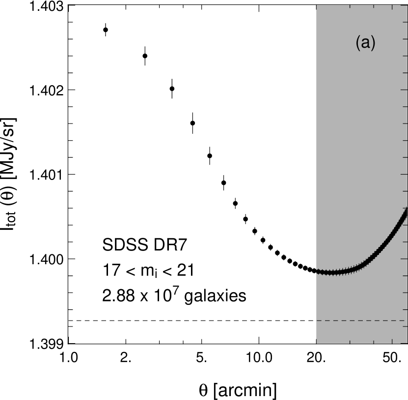
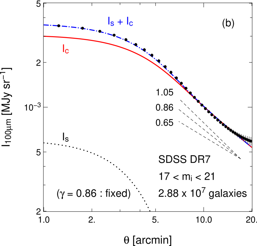
Figure 1: Radial profile of the FIR stacked image of SDSS galaxies. The symbols indicate the radial average of the stacked image and the error bars show rms in each radial bin. (a); Radial profile of the raw stacked image for $\theta<60^{\prime}$ (before subtracting the offset level due to the Galactic dust). Shaded region indicates the data with $\theta>20^{\prime}$ that are not used in the current analysis. (b); Radial profile of the stacked image after subtracting the offset level of $C=1.39927\rm{[MJy\leavevmode\nobreak\ sr^{-1}]}$, which is computed assuming $\gamma=0.86$ and shown as the dashed line in panel a. The lines indicate the best-fits for $I_{\rm s}$ (black dotted), $I_{\rm c}$ (red solid), and $I_{\rm tot}-C$ (blue dot-dashed); see equation (2). Just for reference, we plot the power-laws of $\gamma=0.65$, 0.86 and 1.05 in dashed lines, which covers the ranges of the MSFR result in equation (1).

We adopt the following radial density profile of dust:

$$I_{\rm tot}(\theta)=I_{\rm s}(\theta)+I_{\rm c}(\theta)+C,$$ (2)

where $I_{\rm s}$ and $I_{\rm c}$ represent the contributions from the central single galaxy (single term) and from the clustered neighbor galaxies (clustering term), respectively, and $C$ is the background level of the foreground Galactic dust emission . We assume that the Galactic foreground, $C$, should be uncorrelated with the SDSS galaxies, and thus is assumed to be constant at $\theta<20^{\prime}$.

Since the PSF of SFD/IRAS map is well approximated by Gaussian, $I_{\rm s}(\theta)$ is written as

$$I_{\rm s}(\theta)=I_{{\rm s}0}\exp\left(-\frac{\theta^{2}}{2\sigma^{2}}\right),$$ (3)

where $\sigma=3^{\prime}.1$ is the Gaussian width of PSF.

The clustering term $I_{\rm c}$ is written in terms of $I_{\rm s}$ and angular two-point correlation function (2PCF) of galaxy, $w(\theta)$, as

$$I_{\rm c}(\theta) = \int dm^{\prime}\frac{dN(m^{\prime})}{dm}$$ (4)

$$\leavevmode\nobreak\ \leavevmode\nobreak\ \leavevmode\nobreak\ \times\int d\mathbf{\varphi}I_{\rm s}(\mathbf{\theta}-\mathbf{\varphi};m^{\prime})w(\mathbf{\varphi};m^{\prime}),$$

where $dN(m^{\prime})/dm^{\prime}$ is the differential number count of galaxies (whether or not detected by SDSS) as a function of $m^{\prime}$. We assume that the single term is written as a function of $m_{i}$ alone, therefore the dependence on other physical quantities is neglected. We approximate the angular 2PCF is described as a single power-law in this angular scale (Connolly et al., 2002; Scranton et al., 2002);

$$w(\theta;m^{\prime})=A(m^{\prime})\left(\frac{\theta}{\theta_{0}}\right)^{-\gamma},$$ (5)

where the amplitude $A$ is a function of $m_{i}$, but the index $\gamma$ is assumed to be a constant and independent of $m_{i}$. In this case, equation (4) reduces to

$$I_{\rm c}(\theta)=I_{{\rm c}0}\exp\left(-\frac{\theta^{2}}{2\sigma^{2}}\right){\leavevmode\nobreak\ }_{1}F_{1}\left(1-\frac{\gamma}{2};1;\frac{\theta^{2}}{2\sigma^{2}}\right),$$ (6)

where ${}_{1}F_{1}(a;b;c)$ denotes the confluent hypergeometric function, and

$$I_{{\rm c}0} = 2\pi\sigma^{2}\left(\frac{\varphi_{0}}{\sqrt{2}\sigma}\right)^{\gamma}\Gamma\left(1-\frac{\gamma}{2}\right)$$ (7)

$$\leavevmode\nobreak\ \leavevmode\nobreak\ \leavevmode\nobreak\ \times\int dm^{\prime}I_{{\rm s}0}(m^{\prime})A(m^{\prime})\frac{dN(m^{\prime})}{dm^{\prime}}.$$

We fit the radial profile of the stacked image using equations (2), (3), and (6). In doing so, we do not use equation (7), but treat $I_{{\rm c}0}$ simply as one of the fitting parameters empirically determined from the observed profile. Consistency of the resulting $I_{{\rm c}0}$ with equations (5) and (7) independently measured for SDSS galaxies is an interesting topic (KYS13), which will be discussed in detail elsewhere (Okabe et al. in preparation). We estimate the statistical errors using the jackknife resampling method by dividing the entire SDSS sky area into 400 patches of equal area.

The detected emission profile at small $\theta$ is affected due to the IRAS PSF, and should not be directly compared with the MSFR measurement. Therefore, we use the clustering term, which is relevant for $\theta\gg\sigma$, for the dust temperature constraint in the following Section. In fact, the PSF effect on the clustering term vanishes at large $\theta$ and equation (6) reduces to the power-law as

$$I_{c}(\theta)=\frac{I_{\rm c0}}{\Gamma\left(1-\gamma/2\right)}\left(\frac{\theta}{\sqrt{2}\sigma}\right)^{-\gamma}.$$ (8)

Since we (implicitly) assume here that the mean reddening profile of MSFR, equation (1), is explained in the clustered dust model, the value of $\gamma$ in equation (5) should match the MSFR result. In order to confirm the validity of the assumption, we first choose $I_{{\rm s}0}$, $I_{{\rm c}0}$, $C$, and $\gamma$ as free parameters, and fit to the observed profile imposing $I_{{\rm s}0}\geq 0$ and $I_{{\rm c}0}\geq 0$. The resulting best-fit value, $\gamma=1.07\pm 0.16$, is consistent with that of MSFR, $\gamma=0.86\pm 0.19$ (the other best-fit values include $I_{\rm s0}=0{\rm[MJy\leavevmode\nobreak\ sr^{-1}]}$, $I_{\rm c0}=(3.5\pm 0.4)\times 10^{-3}{\rm[MJy\leavevmode\nobreak\ sr^{-1}]}$, and $C=1.399\pm 0.035{\rm[MJy\leavevmode\nobreak\ sr^{-1}]}$). Indeed as Figure 1 illustrates, the difference among the predicted profiles for $0.65<\gamma<1.05$ is very small for the angular scales of our interest $\theta\gg\sigma$. The departure from the power-law for $I_{\rm c}<6\times 10^{-4}{\rm[MJy\leavevmode\nobreak\ sr^{-1}]}$ is not a problem because it simply reflects the sensitivity to the subtracted offset $C$.

Thus we fix $\gamma=0.86$ in what follows, and obtain the best-fit parameters as $I_{\rm s0}=(6.1\pm 4.0)\times 10^{-4}{\rm[MJy\leavevmode\nobreak\ sr^{-1}]}$, $I_{\rm c0}=(3.1\pm 0.7)\times 10^{-3}{\rm[MJy\leavevmode\nobreak\ sr^{-1}]}$, and $C=1.399\pm 0.035{\rm[MJy\leavevmode\nobreak\ sr^{-1}]}$. The best-fit profile for each component is shown in Figure 1.

The stacked FIR emission profile corresponding to the clustering term for $\gamma=0.86$ is finally given as

$$\langle I_{100\mu{\rm m}}\rangle(\theta)=\frac{(7.0\pm 1.6)\times 10^{-3}}{\rm{MJy\leavevmode\nobreak\ sr^{-1}}}\left(\frac{\theta}{1^{\prime}.0}\right)^{-0.86},$$ (9)

at large $\theta$, which plays a major role in our method proposed in Section 3.3.

We note that while the statistical error of $C$ is much larger than the best-fit values of $I_{\rm s0}$ and $I_{\rm c0}$ themselves, it does not affect the detection significance of the dust emission from SDSS galaxies. In fact, the variance of $C$ simply comes from that of the Galactic dust over the SDSS survey area; the majority of the 400 jackknife subsamples indicates similar signatures of the dust emission, except for the difference of $C$.

It is interesting to note that the observed stacked profile and the prediction from the summation of individual SDSS galaxies indeed agree very well, as mentioned in Section 1. Thus we will proceed further to an independent and complementary analysis in order to constrain the spatial extent of dust in the rest of this section.

3.2 A simple model prediction of the dust emission

While the dust extinction is determined mainly by its column density, the dust emission depends sensitively on its temperature as well. Therefore, if the measured extinction and emission comes from the same dust distribution, their ratio serves as a sensitive measure of the dust temperature. In this subsection, we will explicitly show theoretical expressions for the reddening and emission of dust in a simple model of dust density distribution. Since we are interested in the scales beyond the galactic disk scale, we consider the clustering term alone.

The angular profiles of dust extinction and emission around a galaxy are calculated by integrating the dust surface density $\Sigma_{\rm d}(r_{p},z)$ of nearby galaxies at $z$ separated by the projected distance $r_{p}=d_{A}(z)\theta$ from the central galaxy, where $d_{A}(z)$ is the angular diameter distance at $z$. For simplicity, we assume that the 2-dimensional projected dust surface density responsible for the clustering term is given by a single power-law:

$$\Sigma_{\rm d}(r_{p},z)=\Sigma_{{\rm d}0}(z)\left(\frac{r_{p}}{r_{p,0}}\right)^{-\gamma}.$$ (10)

Throughout the current model, we set the power-law index $\gamma$ as that of the galaxy angular correlation function, equation (5), specifically $\gamma=0.86$ in what follows. Although we neglect the redshift evolution of the correlation length $r_{p,0}$, it is effectively absorbed in $\Sigma_{{\rm d}0}(z)$ as long as $\gamma$ is time-independent as assumed here.

Under the above assumptions, the angular extinction profile of dust at redshift $z$ is written as

$$E_{g-i}(\theta,z) = \frac{2.5}{\ln 10}\left[\tau\left(\theta,\frac{\lambda_{g}}{1+z}\right)-\tau\left(\theta,\frac{\lambda_{i}}{1+z}\right)\right]$$ (11)

$$= \frac{2.5}{\ln 10}\left[\kappa_{\rm ext}\left(\frac{\lambda_{g}}{1+z}\right)-\kappa_{\rm ext}\left(\frac{\lambda_{i}}{1+z}\right)\right]$$

$$\times \Sigma_{\rm d}\big{(}d_{A}(z)\theta,z\big{)},$$

where $\lambda_{g}$ and $\lambda_{i}$ are the rest-frame wavelengths of SDSS $g$ and $i$-bands, respectively, and $\kappa_{\rm ext}(\lambda)$ is the extinction cross-section per unit dust mass at a wavelength of $\lambda$. The average angular extinction profile around SDSS galaxies is then given by

$$\langle E_{g-i}\rangle(\theta) = \frac{2.5}{\ln 10}\left[\int^{\infty}_{0}\frac{dN}{dz}dz\right]^{-1}$$ (12)

$$\times \int^{\infty}_{0}\left[\kappa_{\rm ext}\left(\frac{\lambda_{g}}{1+z}\right)-\kappa_{\rm ext}\left(\frac{\lambda_{i}}{1+z}\right)\right]$$ (13)

$$\times\leavevmode\nobreak\ \Sigma_{\rm d0}(z)\left(\frac{d_{A}(z)\theta}{r_{p,0}}\right)^{-\gamma}\frac{dN}{dz}dz,$$ (14)

where $dN/dz$ is the redshift distribution of SDSS galaxies. Following MSFR, we adopt an approximation (Dodelson et al., 2002):

$$\frac{dN}{dz}\propto z^{2}e^{-(z/0.187)^{1.26}}.$$ (15)

Thus the number-weighted mean redshift of the sample is given by

$$\langle z\rangle=\frac{\int z(dN/dz)dz}{\int(dN/dz)dz}=0.36.$$ (16)

One can similarly compute the angular FIR emission profile around SDSS galaxies. Since the dust emission at $\lambda=100\mu{\rm m}$ is well approximated by the blackbody spectrum, the corresponding surface brightness at redshift $z$ is given as

$$I_{100\mu{\rm m}}(\theta,z,T_{\rm d}) =\frac{1}{(1+z)^{4}}B_{\nu}\left(\frac{100\mu{\rm m}}{1+z},T_{\rm d}\right)$$ (17)

$$\times\kappa_{\rm abs}\left(\frac{{100\mu{\rm m}}}{1+z}\right)\Sigma_{\rm d}\big{(}d_{A}(z)\theta,z\big{)},$$ (18)

where $\kappa_{\rm abs}$ is the absorption cross section per unit dust mass, $B_{\nu}$ is the blackbody spectrum per unit frequency, $T_{\rm d}$ is the dust temperature, which we assume to be independent of $z$, and the same for all SDSS galaxies, and $1/(1+z)^{4}$ comes from the cosmological dimming effect.

The average angular emission profile of SDSS galaxies, which corresponds to $I_{\rm c}(\theta)$ observed by the stacking analysis, is given as

$$\langle I_{100\mu{\rm m}}\rangle(\theta,T_{\rm d})$$ (19)

$$= \left[\int^{\infty}_{0}\frac{dN}{dz}dz\right]^{-1}\leavevmode\nobreak\ \int^{\infty}_{0}\frac{1}{(1+z)^{4}}B_{\nu}\left(\frac{{100\mu{\rm m}}}{1+z},T_{\rm d}\right)$$ (20)

$$\times \kappa_{\rm abs}\left(\frac{{100\mu{\rm m}}}{1+z}\right)\Sigma_{\rm d0}(z)\left(\frac{d_{A}(z)\theta}{r_{p,0}}\right)^{-\gamma}\frac{dN}{dz}dz.$$ (21)

Because we adopt the power-law dust profile, equation (10), the ratio of equation (19) to (12) is independent of $\theta$, and written in terms of $\kappa_{\rm ext}$, $\kappa_{\rm abs}$, and $T_{\rm d}$ alone.

The observed profile of the emission to reddening ratio is shown in Figure 2. The filled circles are plotted using the residual of the emission profile, from which the best-fit single term and the offset level assuming $\gamma=0.86$ are subtracted. The red solid curve shows the ratio of the best-fit clustering term, $I_{\rm c}(\theta)$, with $\gamma=0.86$ to equation (1), and the shaded region indicates its uncertainty due to the statistical error of $I_{\rm c0}$ and the amplitude of equation (1). The uncertainty of the power-law index in equation (1) is not considered here. At small $\theta$, the emission profile is suppressed due to the SFD/IRAS PSF effect, whereas the ratio converges to a constant at large scale. The emission to reddening ratio at large $\theta$ limits is given by equations (1) and (9) as $\langle I_{100\mu{\rm m}}\rangle/\langle E_{g-i}\rangle=4.7\pm 1.6\leavevmode\nobreak\ {\rm[MJy\leavevmode\nobreak\ sr^{-1}mag^{-1}]}$, which corresponds to the shaded regions in Figure 3 below.

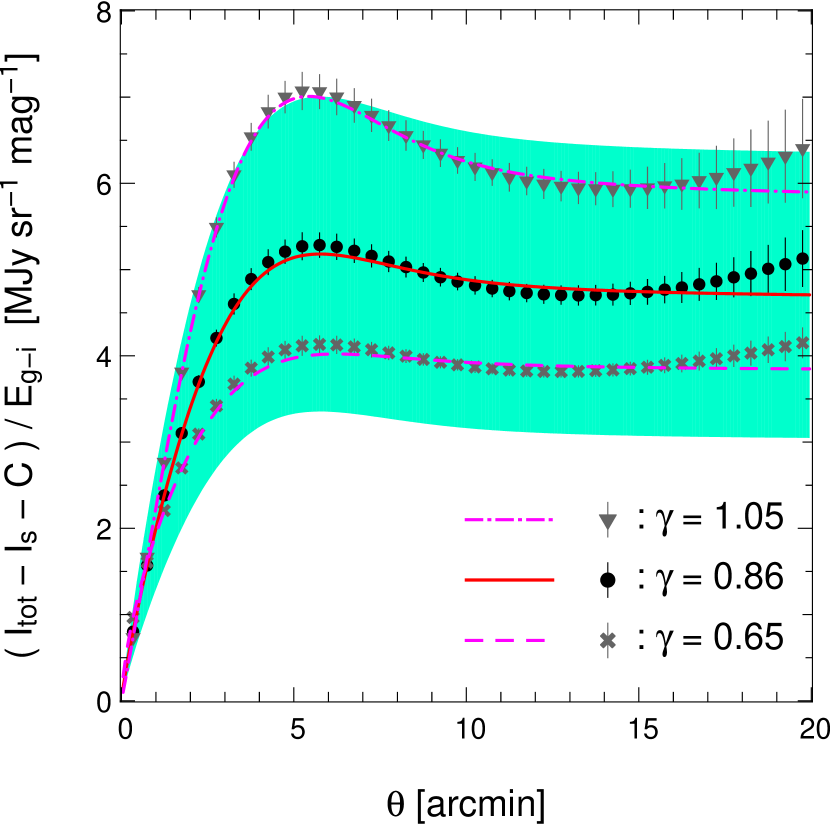
Figure 2: Radial profile of $100\mu{\rm m}$ emission to reddening ratio. Filled circles (black) indicate the observed $100\mu{\rm m}$ emission profile of the stacking analysis divided by the MSFR reddening profile, where the best-fit single term $I_{\rm s}(\theta)$ and the offset level $C$ assuming the 2PCF index as $\gamma=0.86$ are subtracted. Red solid curve is the best-fit profile of the clustering term $I_{\rm c}(\theta)$ with $\gamma=0.86$, divided by $E_{g-i}(\theta)$ of MSFR. Shaded region indicates the uncertainty of the emission to reddening ratio where the statistical error of $I_{\rm c0}$ and the MSFR measurement is taken into account. Crosses (filled triangles) and dashed (dot-dashed) curve indicate the same as filled circles and solid curve, but for $\gamma=0.65\leavevmode\nobreak\ (1.05)$.

We also consider the extent to which this result is sensitive to the choice of the power-law index $\gamma$, which is fixed as 0.86 in the analysis above. We repeat both the fitting to the observed profile and the theoretical calculation of equation (12) and (19), varying the value of $\gamma$ from 0.65 to 1.05. Figure 2 shows the observed emission to reddening ratio for $\gamma=0.65$, $0.86$ and $1.05$. The average ratio changes approximately $\sim 20$ per cent (and its fractional uncertainty is similar to that for the case of $\gamma=0.86$, although it is not shown in Figure 2). We also make sure that the theoretical value from equation (12) and (19) changes by $10$ per cent according to the corresponding change of $\gamma$. Consequently, we find that the uncertainty of dust temperature due to the choice of $\gamma$ is merely $\sim 1$K. This can be neglected comparing with the possible larger systematics due to other many simplifying assumptions.

3.3 Constraints on dust temperature

The solid and dashed lines in Figure 3 indicate the expected emission to extinction ratio as a function of $T_{\rm d}$. We adopt the values of $\kappa_{\rm ext}$ and $\kappa_{\rm abs}$, from the dust model by Weingartner & Draine (2001) for Milky Way ($R_{V}=3.1$) and SMC dust, for solid and dashed lines, respectively.

Here the redshift dependence of $\Sigma_{\rm d0}(z)$ is neglected and assumed to be constant just for simplicity. Indeed we made sure that the $z$-dependence of $\Sigma_{\rm d0}(z)$ does not significantly change the result; if we assume $\Sigma_{\rm d0}(z)\propto(1+z)^{p}$ for instance, the model prediction of $\langle I_{100\mu{\rm m}}\rangle/\langle E_{g-i}\rangle$ changes by $\mp 15$ per cent for $p=\pm 1$, and the dust temperature constraint changes by $\pm 0.2{\rm K}$. The recent measurement of dust mass function by Dunne et al. (2011) found that the cosmic dust mass density in sub-mm galaxies rapidly increases with redshift up to $z\sim 0.5$. Thus the constraint on the dust temperature below may be slightly underestimated.

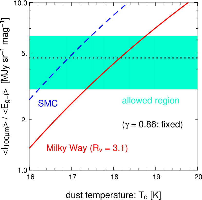
Figure 3: Constraints on the FIR emission to extinction ratio from MSFR and the stacking results (shaded region). Solid and dashed lines indicate the prediction for Milky Way ($R_{V}=3.1$) and SMC dust model (Weingartner & Draine, 2001), respectively. The power-law index of galaxy 2PCF is fixed as $\gamma=0.86$. If $\gamma=0.65$ and $1.05$ is assumed, the allowed region is shifted by $-20$ and $20$ per cent, respectively.

Figure 3 indicates that the dust model predictions and the observed region are consistent if $T_{\rm d}=18.2^{+0.6}_{-0.9}{\rm K}$ for MW dust, and $T_{\rm d}=17.0^{+0.5}_{-0.8}{\rm K}$ for SMC, thus the obtained constraints are almost insensitive to the choice of dust model.

Given several approximations adopted in our simple model, the quoted statistical errors may underestimate the real uncertainty of the dust temperature. Nevertheless it is encouraging that the derived dust temperature is in good agreement with that of the typical cold component of the ISD (Schlegel, Finkbeiner & Davis, 1998; Dunne et al., 2011; Clemens et al., 2013). While this result is reasonably consistent with the ISD model, it is premature to conclude that the observed dust profile is explained by the sum of the dust in the central parts of individual galaxies. Our dust model above is based on a single-temperature component, and the extended dust component around a galaxy may have a substantially lower temperature. In this case, the emission flux is much smaller while the reddening amplitude remains almost the same.

Therefore we consider a two-component dust model below. In order to keep the same surface density profile of dust, we assume that the two components, corresponding to ISD and CGD, share the identical spatial distribution, but they are allowed to have different temperatures $T_{\rm ISD}$ and $T_{\rm CGD}$. While this is still a very simple model, we would like to proceed with it because the low-angular resolution of IRAS images make it difficult to distingush the density profile less than $\sigma=3^{\prime}.1$. In any case the purpose of the current paper is to propose a new method to constrain the dust density and temperature, which will be improved significantly later theoretically and observationally.

In the above spirit, we replace equation (10) by

$$\Sigma_{\rm d}(r_{p},z)=[\Sigma_{{\rm d}0,{\rm ISD}}(z)+\Sigma_{{\rm d}0,{\rm CGD}}(z)]\left(\frac{r_{p}}{r_{p,0}}\right)^{-\gamma}.$$ (22)

Then the observed FIR emission to extinction ratio becomes

$$\bigg{[}\frac{\langle I_{100\mu{\rm m}}\rangle}{\langle E_{g-i}\rangle}\bigg{]}_{\rm obs}=$$ (23)

$$\leavevmode\nobreak\ \frac{f_{\rm ISD}\langle I_{100\mu{\rm m}}\rangle(T_{\rm ISD})+(1-f_{\rm ISD})\langle I_{100\mu{\rm m}}\rangle(T_{\rm CGD})}{\langle E_{g-i}\rangle},$$ (24)

at large $\theta$, where $\langle E_{g-i}\rangle$ and $\langle I_{100\mu{\rm m}}\rangle(T)$ in the right-hand-side are given by equation (12) and (19), respectively. We further assume that the fraction of the ISD mass to the total mass:

$$f_{\rm ISD}=\frac{\Sigma_{{\rm d}0,{\rm ISD}}}{\Sigma_{{\rm d}0,{\rm ISD}}+\Sigma_{{\rm d}0,{\rm CGD}}}$$ (25)

is independent of redshift. Thus the observed value of $\langle I_{100\mu{\rm m}}\rangle/\langle E_{g-i}\rangle$ provides a constraint on $f_{\rm ISD}$ for given values of $T_{\rm ISD}$ and $T_{\rm CGD}$. The preceding analysis corresponds to $f_{\rm ISD}=1$.

The temperature of the CGD is fairly uncertain because of the unknown heating mechanism of the CGD. If the heating source of the CGD is dominated by the cosmic UV background, which is lower than the interstellar radiation field in the solar neighborhood by two orders of magnitude (Madau & Pozzetti, 2000; Gardner et al., 2000; Xu et al., 2005), we obtain $T_{\rm CGD}=10{\rm K}$ following (Draine & Lee, 1984; Draine, 2011). On the other hand, Yamada & Kitayama (2005) assume the collisional heating mechanism by hot plasma and the efficient injection of dust grains outside the galactic disk. In this case, they suggested a possibility that the dust temperature reaches even $\sim 30{\rm K}$.

The abundance of such possible high-temparature CGD, however, is severly constrained by the observed data. (Clark et al., 2015) fitted the SED of dust-selected galaxies, and found that the majority of them have cool and warm dust components with $T\sim(10$–$20)$K and $>30$K. The mass of the cool component is typically 100 times larger than that of the warm component. While the two components may correspond to the two-temperature phases in ISD, the estimated mass ratio can be also interpreted to put a severe constraint on the presence of the hot CGD with $T\sim 30$K. Furthermore, Draine et al. (2014) reported that the dust temperature near the edge of M31 disk is $15{\rm K}$. Thus the dust temperature in the outskirt is naturally expected to be much lower.

For those reasons, we adopt $T_{\rm CGD}=10{\rm K}$ in what follows. We also confirm that the result below does not change as long as $T_{\rm CGD}$ is lower than $10$K.

Figure 4 shows the constraint on $T_{\rm ISD}$ and $f_{\rm ISD}$ from the observed value of $\langle I_{100\mu{\rm m}}\rangle/\langle E_{g-i}\rangle$. Due to the strong degeneracy between the two parameters, the constraint allows a wide range of the ISD mass fraction, even as small as $f_{\rm ISD}\sim 10^{-2}$ if $T_{\rm ISD}=30{\rm K}$. Thus the measurement of the mean dust temperature of the central parts of galaxies $T_{\rm ISD}$ is crucial in distinguishing the origin of the spatial extension of dust. Indeed, the average temperature of the ISD varies depending on the properties of the galaxies, and can be as high as $\sim 40{\rm K}$ (Skibba et al., 2011). In this respect, the current data do not exclude a possibility that a substantial amount of the CGD exists, as suggested by MSFR and the subsequent studies (e.g., Fukugita, 2011; Ménard & Fukugita, 2012; Peek, Ménard, & Corrales, 2014). Nevertheless further improvements in model predictions and the observations in future would put more stringent constraints on the spatial extent of dust through the measurement of dust temperature as we proposed in this paper.

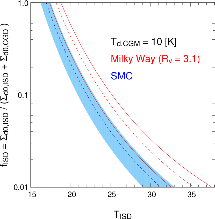
Figure 4: Constraints on the ISD temperature, $T_{\rm ISD}$, and the mass fraction of the ISD to the sum of the ISD and CGD. We assume that the CGD temperature as $T_{\rm CGD}=10\leavevmode\nobreak\ {\rm K}$. Red curves and blue shaded region indicate the constraint adopting Milky Way ($R_{V}=3.1$) and SMC dust model (Weingartner & Draine, 2001), respectively.

4 Summary & Conclusions

The spatial distribution of dust is of fundamental importance in understanding the star formation and metal circulation history in the universe. It is also crucial in correcting for the magnitude of distant objects due to the resulting reddening/extinction (Aguirre, 1999; Ménard et al., 2010b; Fang et al., 2011).

In a previous paper (Kashiwagi et al., 2013), we have detected the FIR dust emission from SDSS galaxies via their image stacking analysis. We found that the amount of dust emission is largely responsible for the observed anomaly in the surface density of SDSS galaxies as a function of the SFD extinction (Yahata et al., 2007; Kashiwagi et al., 2015). Our previous analysis implicitly assumed that the dust of each galaxy is locally confined in the galactic disk scale, and that the observed FIR emission within the large PSF width (FWHM$=6^{\prime}.1$) is simply given as a sum of contributions of individual galaxies (corresponding to the ISD model in the present paper). In contrast, the dust around a galaxy may be indeed spatially extended up to $\sim 1$Mpc (CGD model), as claimed by Ménard et al. (2010a) and more recently by Peek, Ménard, & Corrales (2014) through the correlation of background object colors against the separation length of foreground galaxies.

In order to distinguish between the ISD and CGD models, we propose a new method that constrains the temperature of dust by combining the absorption (detected through reddening of quasars) and emission (detected through the stacking of galaxies) features. Assuming that the nature of galactic dust is described by those of MW and SMC, we find that the observed dust is reasonably explained in terms of ISD model if the dust temperature of the central parts of individual galaxies, $T_{\rm ISD}$, is approximately 20K. The estimated temperature is consistent with that of the galactic dust in the central region, but may be higher than that predicted for CGD, if it is heated by UV background alone. On the other hand, the substantial amount of dust may reside far outside the galactic disks if $T_{\rm ISD}$ is much higher than 20K.

Given several simplification and approximations that we adopted in the present simple model analysis, the associated error-bars of the derived dust temperature is fairly uncertain. Nevertheless we would like to emphasize that the main purpose of the present paper is to propose a new observational method to diagnose the nature of galactic dust. Therefore we do not discuss the interpretation of the present preliminary result.

Our proposed method should be, and indeed can be, improved in many ways; the two components of dust may have different spatial density profiles in addition to the different temperatures. The redshift evolution of the temperature and amount of dust may be included in the theoretical models. In addition, the line-of-sights of our emission and reddening measurements may not be exactly the same. Since quasars behind the heavily extincted line-of-sights may not be identified in the SDSS photometric catalogue, the reddening measurement may systematically underestimate the real optical depths while the emission is largely free from the bias. Those improvements of the theoretical models and the effect of the possible selection bias need to be investigated, for instance, with mock simulations, which is beyond the scope of the present paper.

The observational data and analysis can be also improved in future. The dust temperature would vary depending on the different properties of galaxies, and the amount of dust emission should depend on the morphology of galaxies. The image stacking analysis with better angular resolutions and in multi-wavelengths would significantly improve the observational data. Indeed current result is significantly limited by the poor angular resolution of IRAS. In those respects, the higher-angular-resolution and multi-band far-infrared data by AKARI (Murakami et al., 2007) are very promising. We plan to present elsewhere more detailed and systematic results using the AKARI data (Okabe et al. in preparation).

We thank Brice Ménard, Bruce T. Draine, Masato Shirasaki, and Tetsu Kitayama for useful discussions. We also appreciate several comments by an anonymous referee that motivated us to consider the two-temperature dust model as well. This work is supported in part from the Grant-in-Aid No. 20340041 by the Japan Society for the Promotion of Science. Y.S. and T.K. gratefully acknowledge supports from the Global Scholars Program of Princeton University and from Global Center for Excellence for Physical Science Frontier at the University of Tokyo, respectively.

Data analysis were in part carried out on common use data analysis computer system at the Astronomy Data Center, ADC, of the National Astronomical Observatory of Japan.

Funding for the SDSS and SDSS-II has been provided by the Alfred P. Sloan Foundation, the Participating Institutions, the National Science Foundation, the U.S. Department of Energy, the National Aeronautics and Space Administration, the Japanese Monbukagakusho, the Max Planck Society, and the Higher Education Funding Council for England. The SDSS Web Site is http://www.sdss.org/.

The SDSS and SDSS-II are managed by the Astrophysical Research Consortium for the Participating Institutions. The Participating Institutions are the American Museum of Natural History, Astrophysical Institute Potsdam, University of Basel, Cambridge University, Case Western Reserve University, University of Chicago, Drexel University, Fermilab, the Institute for Advanced Study, the Japan Participation Group, Johns Hopkins University, the Joint Institute for Nuclear Astrophysics, the Kavli Institute for Particle Astrophysics and Cosmology, the Korean Scientist Group, the Chinese Academy of Sciences (LAMOST), Los Alamos National Laboratory, the Max-Planck-Institute for Astronomy (MPIA), the Max-Planck-Institute for Astrophysics (MPA), New Mexico State University, Ohio State University, University of Pittsburgh, University of Portsmouth, Princeton University, the United States Naval Observatory, and the University of Washington.

References

- Aguirre (1999) Aguirre, A. N. ApJL, 1999, 512, 19
- Clark et al. (2015) Clark, C. J. R., et al. 2015, astro-ph/1502.03843
- Clemens et al. (2013) Clemens, M. S., et al. MNRAS, 2013, 433, 695
- Chelouche et al. (2007) Chelouche, D., Koester, B. P., & Bowen, D. V. 2007 ApJ, 671, 97
- Connolly et al. (2002) Connolly, A. J., et al. 2002, ApJ, 579, 42
- Dodelson et al. (2002) Dodelson, S., et al. 2002, ApJ, 572, 140
- Draine & Lee (1984) Draine, B. T., & Lee, H. M. 1984, ApJ, 285, 89
- Draine (2011) Draine, B., T. 2011, Physics of the Interstellar and Intergalactic Medium (Princeton, NJ: Princeton University Press)
- Draine et al. (2014) Draine, B., T. et al. 2014, ApJ, 780, 172
- Dunne et al. (2011) Dunne, L., et al. 2011, MNRAS, 417, 1510
- Fang et al. (2011) Fang, W., Hui. L., Ménard, B., May, M., & Scranton, R. 2011, PhRvD, 84, 3012
- Fukugita et al. (1996) Fukugita, M., Ichikawa, T., Gunn, J. E., Doi, M., Shimasaku, K. & Schneider, D. P. 1996, AJ, 111, 1748
- Fukugita (2011) Fukugita, M., 2011, astro-ph/1103.4191
- Gardner et al. (2000) Gardner, J. P., Brown, T. M., & Ferguson, H. C., 2000, ApJ, 542, 79
- Gunn et al. (1998) Gunn, J. E., et al. 1998, AJ, 116, 3040
- Gunn et al. (2006) Gunn, J. E., et al. 2006, AJ, 131, 2332
- Gutierrez & Lopez-Corredoira (2014) Gutierrez, C. M., & Lopez-Corredoira, M. 2014, A&A, 571, 66
- Hogg et al. (2001) Hogg, D. W., Finkbeiner, D. P., Schlegel, D. J. & Gunn, J. E. 2001, AJ, 122, 2129
- Ivezic et al. (2004) Ivezić, Ž., et al. 2004, Astronomische Nachrichten, 325, 583
- Kaneda et al. (2009) Kaneda, H., Yamagishi, M., Suzuki, T., & Onaka, T. 2009, ApJ, 698, 125
- Kashiwagi et al. (2013) Kashiwagi, T., Yahata, K., & Suto, Y. 2013, PASJ, 65, 43 (KYS13)
- Kashiwagi et al. (2015) Kashiwagi, T., Suto, Y., Taruya, A., Kayo, I., Nishimichi, T., & Yahata, K. 2015, ApJ, 799, 132
- Kitayama et al. (2009) Kitayama, T., et al. 2009, ApJ, 695,1191
- Madau & Pozzetti (2000) Madau, P., & Pozzetti, L. 2000, MNRAS, 312, 9
- McGee & Balogh (2010) McGee, S. L., & Balogh, M, L. 2010 MNRAS, 405, 2069
- Ménard et al. (2010a) Ménard, B., Scranton, R., Fukugita, M., & Richards, G. 2010a, MNRAS, 405, 1025 (MSFR)
- Ménard et al. (2010b) Ménard, B., Kilbinger. M., & Scranton, R. 2010b, MNRAS, 406, 1815
- Ménard & Fukugita (2012) Ménard, B. and Fukugita, M. 2012, ApJ, 754, 116
- Montier & Giard (2005) Montier, L. A., & Giard, M. 2005, A&A, 439, 35
- Muller et al. (2008) Muller, S., Wu, S. Y., Hsieh, B. C., González, R. A., Loinard, L., Yee, H. K. C., & Gladders, M. D. 2008, ApJ, 680, 975
- Murakami et al. (2007) Murakami, H., et al. 2007, PASJ, 59, 369
- Padmanabhan et al. (2008) Padmanabhan, N., et al. 2008, ApJ, 674, 1217
- Peek, Ménard, & Corrales (2014) Peek, J., E., G., Ménard, B., & Corrales, L. 2014, arXiv:1411.3333
- Pier et al. (2003) Pier, J. R., Munn, J. A., Hindsley, R. B., Hennessy, G. S., Kent, S. M., Lupton, R. H., & Ivezić, Ž. 2003, AJ, 125, 1559
- Schlegel, Finkbeiner & Davis (1998) Schlegel, D., Finkbeiner, D., & Davis, M. 1998 AJ, 500, 525
- Scranton et al. (2002) Scranton, R., et al. 2002, ApJ, 579, 48.
- Skibba et al. (2011) Skibba, R. A., et al. 2011, ApJ, 738, 89
- Smith et al. (2002) Smith, J. A., et al. 2002, AJ, 123, 2121
- Stoughton et al. (2002) Stoughton, C., et al. 2002, AJ, 123, 485
- Stickel et al. (1998) Stickel, M., Lemke, D., Mattila, K., Haikala, L. K., &Haas, M. 1998, A&A, 329, 55
- Stickel et al. (2002) Stickel, M., Klaas, U., Lemke, D., & Mattila, K. A&A, 2002, 383, 367
- Tucker et al. (2006) Tucker, D. L., et al. 2006, Astronomische Nachrichten, 327, 821
- Weingartner & Draine (2001) Weingartner, J. C., & Draine, B. T. 2001, ApJ, 548, 296
- Xu et al. (2005) Xu, C., K., Donas, J., Arnouts, S., et al. 2005, ApJ, 619, 11
- Yahata et al. (2007) Yahata, K., Yonehara, A., Suto, Y., Turner, E.L., Broadhurst, T., & Finkbeiner, D. 2007, PASJ, 59, 205 (Y07)
- Yamada & Kitayama (2005) Yamada, K., & Kitayama, T. 2005, PASJ, 57, 611
- York et al. (2000) York, D. G., et al. 2000, AJ, 120, 1579
- Zaritsky (1994) Zaritsky, D. 1994, AJ, 108, 1619
- Zwicky (1962) Zwicky, F. 1962, in McVittie G. C., ed., Proc. IAU Symp. 15, Problems of Extra-Galactic Research. Macmillan, New York, p. 347